Article

Characterizing Land Use/Land Cover Using Multi-Sensor Time Series from the Perspective of Land Surface Phenology

by
Lan H. Nguyen
1 and
Geoffrey M. Henebry
2,3,*
1
Geospatial Sciences Center of Excellence, South Dakota State University, Brookings, SD 57007, USA
2
Department of Geography, Environment, and Spatial Sciences, Michigan State University, East Lansing, MI 48824, USA
3
Center for Global Change and Earth Observations, Michigan State University, East Lansing, MI 48823, USA
*
Author to whom correspondence should be addressed.
Remote Sens. 2019, 11(14), 1677; https://doi.org/10.3390/rs11141677
Submission received: 7 June 2019 / Revised: 11 July 2019 / Accepted: 13 July 2019 / Published: 15 July 2019
(This article belongs to the Special Issue Remote Sensing for Crop Mapping)

Abstract

:
Due to a rapid increase in accessible Earth observation data coupled with high computing and storage capabilities, multiple efforts over the past few years have aimed to map land use/land cover using image time series with promising outcomes. Here, we evaluate the comparative performance of alternative land cover classifications generated by using only (1) phenological metrics derived from either of two land surface phenology models, or (2) a suite of spectral band percentiles and normalized ratios (spectral variables), or (3) a combination of phenological metrics and spectral variables. First, several annual time series of remotely sensed data were assembled: Accumulated growing degree-days (AGDD) from the MODerate resolution Imaging Spectroradiometer (MODIS) 8-day land surface temperature products, 2-band Enhanced Vegetation Index (EVI2), and the spectral variables from the Harmonized Landsat Sentinel-2, as well as from the U.S. Landsat Analysis Ready Data surface reflectance products. Then, at each pixel, EVI2 time series were fitted using two different land surface phenology models: The Convex Quadratic model (CxQ), in which EVI2 = f(AGDD) and the Hybrid Piecewise Logistic Model (HPLM), in which EVI2 = f(day of year). Phenometrics and spectral variables were submitted separately and together to Random Forest Classifiers (RFC) to depict land use/land cover in Roberts County, South Dakota. HPLM RFC models showed slightly better accuracy than CxQ RFC models (about 1% relative higher in overall accuracy). Compared to phenometrically-based RFC models, spectrally-based RFC models yielded more accurate land cover maps, especially for non-crop cover types. However, the RFC models built from spectral variables could not accurately classify the wheat class, which contained mostly spring wheat with some fields in durum or winter varieties. The most accurate RFC models were obtained when using both phenometrics and spectral variables as inputs. The combined-variable RFC models overcame weaknesses of both phenometrically-based classification (low accuracy for non-vegetated covers) and spectrally-based classification (low accuracy for wheat). The analysis of important variables indicated that land cover classification for this study area was strongly driven by variables related to the initial green-up phase of seasonal growth and maximum fitted EVI2. For a deeper evaluation of RFC performance, RFC classifications were also executed with several alternative sampling scenarios, including different spatiotemporal filters to improve accuracy of sample pools and different sample sizes. Results indicated that a sample pool with less filtering yielded the most accurate predicted land cover map and a stratified random sample dataset covering approximately 0.25% or more of the study area were required to achieve an accurate land cover map. In case of data scarcity, a smaller dataset might be acceptable, but should not smaller than 0.05% of the study area.

Graphical Abstract

1. Introduction

Knowledge about land use/land cover (LULC) is fundamental for natural resource management, agricultural policy making, and regional and urban planning. Most reliable data sources for LULC information are periodic surveys from governmental agencies, e.g., the National Resource Inventory and the National Agricultural Statistics Service (NASS), both in the United States Department of Agriculture (USDA) [1,2]. However, those datasets often lack spatial and temporal details, which prevents a comprehensive analysis of land change. Remote sensing technology can complement field observations and surveys. Conventional classification approaches, such as those applied in the National Land Cover Dataset (NLCD) [3,4,5] or the Cropland Data Layer (CDL) [6], were developed in an era of data scarcity and limited computational power and data storage. Thus, they have focused on mapping annual land cover from multispectral data from one or just a few image dates. However, in areas with frequent morning cloud cover, collecting even a few cloud-free scenes over a year can be challenging. The recent rapid increase of accessible Earth observation data coupled with improved computing and storage capabilities is leading to the emergence of methods for mapping land cover using multi-date imagery and dense image time series [7]. Compared to the traditional approach, the use of image time series often improves classification accuracy by incorporating both spectral and temporal profiles [8,9,10].
Land surface phenology (LSP) has been a useful approach to characterize seasonal vegetation dynamics on vegetation index time series [11]. Over the past few years, several efforts have been made to map LULC using phenological metrics derived from satellite image time series with promising outcomes [12,13,14,15,16,17,18]. Due to the relatively low return interval of orbital sensors with spatial resolutions finer than 50 m, many studies—with notable exceptions [13,16,18]—have relied on MODIS time series to capture phenological characteristics of land surfaces, thus often producing cover maps at spatial resolutions (e.g., 250–1000 m) that are coarse relative to human land uses, such as agriculture and settlements. To overcome limited temporal coverage of Landsat-like data and map land covers at finer spatial resolutions, Jia et al. [13] and Kong et al. [16] fused the MODIS Normalized Different Vegetation Index (NDVI) [19] with Landsat and Gaofen-1 NDVI time series, respectively. Although each produced land cover maps at finer spatial resolution (30 m for Landsat and 16 m for GF-1), neither Jia et al. [13] nor Kong et al. [16] were able to map more than Level-1 NLCD Land Cover Classification System, except for coniferous and broadleaf forest in Kong et al. [16] (Level-2 NLCD).
In 2016, the United States Geological Survey reorganized the Landsat archive into a tiered collection, namely the Landsat Collections, to facilitate time series analysis and data stacking [20]. Taking advantage of the Landsat Collections data, Nguyen et al. [18] performed a phenometrically-based classification for sample areas in South Dakota using all available Tier-1 (highest quality) images from Landsat 5 Thematic Mapper (TM), Landsat 7 Enhanced Thematic Mapper Plus (ETM+), and Landsat 8 Operational Land Imager (OLI). At each pixel, an Enhanced Vegetation Index (EVI) time series calculated from Landsat Collections data was simulated as a convex quadratic function of accumulated growing degree-days (AGDD), i.e., a measure of accumulated heat from January 1 onward whenever the average temperature exceeded 0° Celsius. Results showed that classification using only phenometrics generated from the fitted model could accurately map broad thematic land cover classes (water, developed, grassland) as well as commodity crops (corn/maize, soybean, wheat) in Codington and Roberts counties in South Dakota for two years (2012 and 2014). However, they also pointed out some challenges of the phenometrically-based classification. First, the classification accuracy varied, since the form of the chosen land surface phenology (LSP) model might be more suitable for some certain vegetation types than others. Second, the phenometrically-based classification performed well only for vegetated classes, particularly crops. Third, many cloud/snow/shadow-free observations were needed at each pixel over a year to fit the LSP model well and to avoid data gaps in the predicted land cover map. Regarding the last point, they [18] also showed that an adequate number of observations could be gathered by combining data from multiple comparable sensors, especially in sidelap zones of Landsat swaths. Finally, in addition to pointing out the challenges of classification based on phenometrics, Nguyen et al. [18] also discussed the potential opportunity to improve classification accuracy by incorporating both phenological and spectral information.
Here, we explored the challenges of the phenometrically-based classification and a potential way to improve classification accuracy, as demonstrated in [18]. This study focused on evaluating the performance of alternative land cover classifications using either (1) only phenological metrics derived from either of different land surface phenology (LSP) models: The Convex Quadratic Model, in which EVI2 = f(AGDD) [11,21] and the Hybrid Piecewise Logistic Model, in which EVI2 = f(day of year) [22], or (2) a suite of spectral band percentiles and normalized ratios (spectral variables), or (3) both phenological metrics and spectral variables. In our evaluation, we addressed three research questions. The first question was whether the maps from the phenometrics were more accurate than maps from spectral variables alone. As land surface phenology has been a useful tool to characterize the dynamics of the vegetated land surface [11], we hypothesized that land cover classifications using only phenometrics could be more accurate for vegetated land covers, especially for commodity crops, than those using only spectral variables. The second question asked which set of phenometrics—derived either from the Convex Quadratic Model (CxQ) or from the Hybrid Piecewise Logistic Model (HPLM)—performed better. In the temperate ecosystem, plant development is sensitive to variation in temperature. We hypothesized, therefore, that the Convex Quadratic Model, which links vegetation growth with the progression of thermal time, would be better suited to land cover classification of our study area in northeastern South Dakota. The third question asked whether combining the phenometrics and spectral variables would result in superior performance. Studies have indicated that classification accuracies were improved by incorporating phenological features [13,16]. Thus, we hypothesized that classification using a combination of spectral variables and phenometrics would be consistently more accurate than using only phenometrics or spectral variables. To build a more complete picture of classification performance, we ran Random Forest Classifiers (RFC) with different sampling scenarios and sets of input variables.
First, three annual time series of remotely sensed data were constructed, including accumulated growing degree-days from the MODIS 8-day composites of land surface temperatures and 2-band Enhanced Vegetation Index (EVI2) [23] and spectral variables from surface reflectance products from (1) Landsat Analysis Ready Data (ARD) and (2) Harmonized Landsat Sentinel-2 (HLS) data, separately. At each pixel, EVI2 time series were then fitted to the LSP models, CxQ or HPLM. Phenometrics derived from the fitted LSP models as well as spectral variables were submitted individually and in combination to RFC to map land use/land cover of the study area. Accuracy assessments for both RFC models and predicted land cover maps were reported using both conventional accuracy metrics (overall, producer’s, and user’s accuracies) [24] and alternatives for kappa [25].
Our assessment of classification performance is two-fold. First, RFC model performance was evaluated by submitting different input datasets randomly generated from the CDL. Accuracy comparisons between classification scenarios were tested by both Mann–Whitney U [26] and equivalence tests [27,28]. These two tests are based on opposite but complementary evaluation perspectives. The nonparametric U test indicates whether the two sets of accuracy metrics are statistically different, regardless how difference magnitude. The equivalence test, on the other hand, examines whether differences fall within a certain user-defined threshold and, thus, deemed equivalent or are large enough to be deemed not equivalent. The second step was to compare the predicted land cover maps with the CDL.

2. Data and Study Area

2.1. Study Area

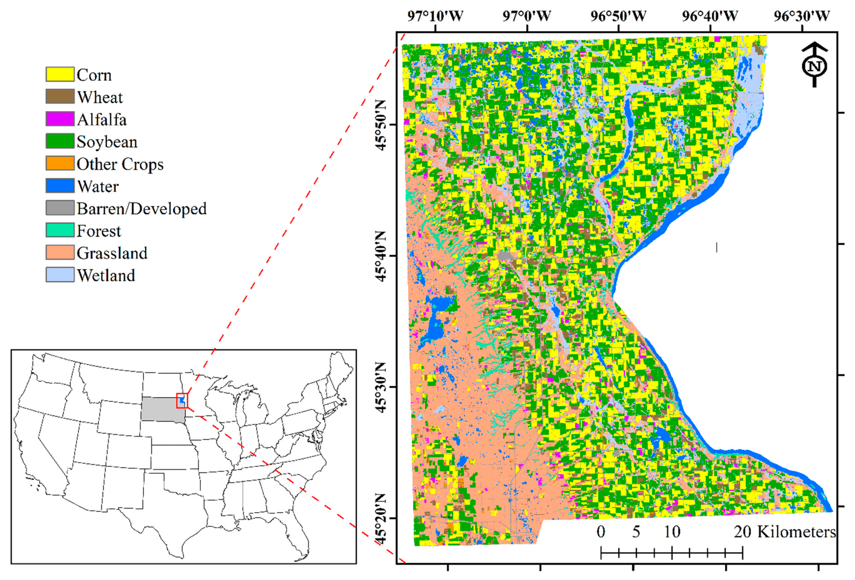
The proposed classification exercise was demonstrated for Roberts County, South Dakota (SD), in two years, 2016 and 2017. Roberts County is at the northeastern corner of South Dakota with a total area of 2940 km2 and a current population of approximately 10,000. According to 2016 CDL (Figure 1), cropland is a dominant land cover in Roberts County, accounting for approximately 53.3% of the county area. Other cover types in the County include grassland (25.9%), wetland (8.9%), water (5.2%), barren/developed (4.4%), and forest (2.2%). The County falls within overlap zones of Landsat paths, which allows retrieval of more cloud-free observations.

2.2. Input Data

2.2.1. Landsat Analysis Ready Data

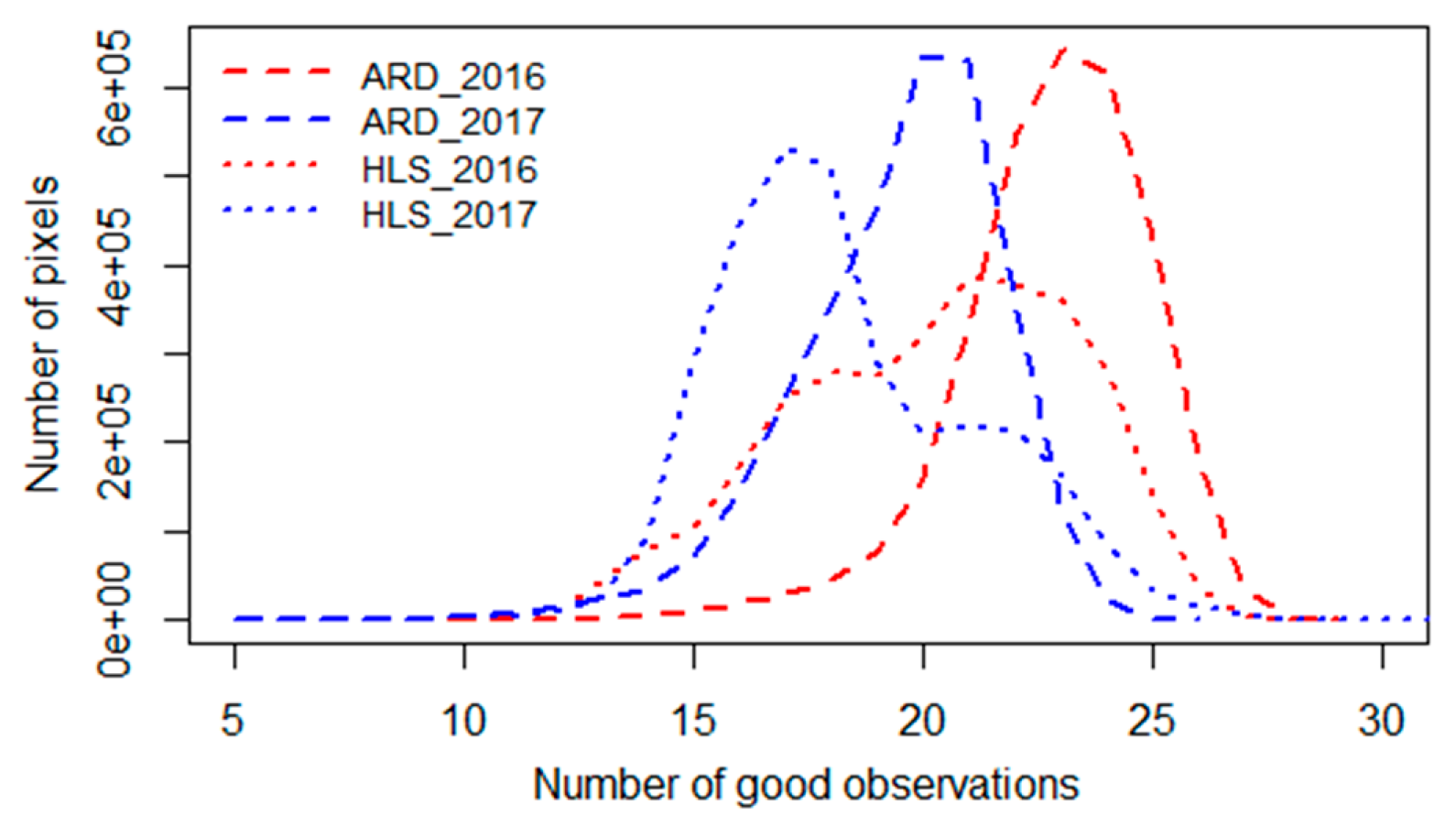
The Landsat Analysis Ready Data (ARD) products from the US Geological Survey are designed to reduce the amount of data preparation for scientists and to facilitate time series analysis by generating data at the highest scientific standards required for direct use in applications [29]. Landsat Collection 1 Level-1 scenes serve as the input for generating all ARD products. The ARD dataset is defined in the Albers Equal Area (AEA) projection and World Geodetic System 1984 datum (WGS84). The products are distributed in 150 × 150 km tiles instead of the traditional Landsat swaths in the WRS-2 path-row coordinate system. Both Landsat 7 and Landsat 8 images in the ARD surface reflectance (SR) product were used. On average, there are 22.8 and 19.5 ARD observations per pixel for 2016 and 2017, respectively (Figure 2).

2.2.2. Harmonized Landsat Sentinel-2

The Harmonized Landsat and Sentinel-2 (HLS) product suite is a combined surface reflectance dataset consisting of observations from both the Landsat 8 Operational Land Imager and Sentinel-2 Multi-Spectral Instrument (MSI) [30]. We used two products from HLS version 1.4: (1) S30—SR derived from Sentinel-2 MSI L1C data and resampled to 30m and (2) L30—30 m SR derived from Landsat-8 OLI L1T data. Both S30 and L30 products provide nadir BRDF-adjusted (Bidirectional Reflectance Distribution Function) reflectance (NBAR) data gridded with the Sentinel-2 tiling system in Universal Transverse Mercator (UTM) projection and World Geodetic System 1984 datum (WGS84). The Sentinel-2 MSI radiometry is adjusted to mimic the spectral bandpasses of Landsat 8 OLI for visible, near infrared, and shortwave infrared bands. On average, there are 20.2 and 18.3 HLS observations per pixel for 2016 and 2017, respectively (Figure 2).

2.2.3. MODIS Land Surface Temperature

We used the Collection 6 MODIS level-3 land surface temperature (LST) 8-day composites at 1000 m spatial resolution from both Aqua (MYD11A2) and Terra (MOD11A2) satellites [31,32]. The MODIS LST data are provided in a sinusoidal grid format and display the mean clear-sky LST in Kelvin observed during the 8-day compositing period. All MODIS data were reprojected and resampled to 30 m using bilinear interpolation into UTM zone 14N to work with the HLS data and into AEA projection to work with the ARD. The LST time series were converted from Kelvin to degrees Celsius for calculation of thermal time used in the LSP modeling.

2.2.4. Cropland Data Layer

The USDA Cropland Data Layer (CDL) is a crop-specific land cover raster created annually for the continental United States by the NASS using moderate resolution satellite imagery and extensive agricultural ground observations [33]. It is distributed in AEA projection and North American 1983 datum (NAD83). The CDL was first produced in 1997 for North Dakota but has covered the contiguous US yearly only since 2008. The product has approximately 130 classes and a spatial resolution of 30 m at best. We regrouped the CDL layers into ten classes (Table S1) and then used this reclassified data to generate sample datasets for input to the RFCs. The reclassified CDL layer also provided a reference against which to evaluate the predicted land cover maps. To work with HLS data, the CDL data were reprojected into UTM zone 14N. Due to differences in the original projections and data, the reclassified CDL, ARD, and HLS pixels are not perfectly co-aligned. While offsets between the CDL and ARD pixels are only about 3 m in both latitude and longitude directions, offsets between the CDL and HLS pixels are 15 m (half pixel) in each direction. We did not resample these data into a common grid, as this step would introduce another source of uncertainty into the analysis.

3. Methods

3.1. Land Surface Phenology Modeling

3.1.1. EVI2 time series from ARD and HLS surface reflectance

The two-band Enhanced Vegetation Index (EVI2) was calculated from ARD and HLS surface reflectance products (red—R and near infrared—NIR bands) using Equation (1) [23]. EVI2 was chosen over the more commonly used Normalized Difference Vegetation Index (NDVI) to avoid the well-known loss of sensitivity that NDVI experiences with denser canopies. EVI2 performs similarly to its predecessor, the 3-band EVI, especially with continuing advancements in atmosphere corrections. Poor-quality observations—snow, high confidence cloud, or cloud shadow pixels—were all masked out using quality control layers delivered with the ARD and HLS products. EVI2 values outside the valid range (from 0 to 1) were also excluded. The remaining “good” EVI2 values at each pixel were then stacked in chronological order from the first day of the year (DOY = 1) to the final day of the year (DOY = 365 or 366 in leap years).
EVI 2 = 2.5   ( NIR R ) ( NIR + 2.4 R + 1 )

3.1.2. AGDD time series from MODIS LST

From MODIS LST, we calculated the accumulated growing degree-days (AGDD) as follows:
GDD t = max { T max ,   t + T min ,   t 2 , 0 } ,
AGDD t = AGDD t 1 + ( 8 × GDD t ) ,
where GDDt is the growing degree-days for compositing period (t is an integer ≥ 1), Tmax,t and Tmin,t are the highest and lowest LST values from available MODIS observations from both Aqua and Terra during the compositing period, assuming that AGDD0 = 0. Since the compositing period is 8 days, we multiplied the GDD by 8 to achieve a proportional accumulation of GDD for each of the 46 composites per year.

3.1.3. Convex Quadratic Model

We fitted the EVI2 time series as a quadratic function of AGDD (Equation (4)) using the process described in [18]:
EVI 2 = α + β × AGDD γ × AGDD 2 ,
where α, β, and γ (alpha, beta, and gamma, respectively) are the parameter coefficients to be fitted. Alpha—a constant component—directly regulates the peak EVI2 value over the growing season, as a changing value of alpha solely would move the fitted curve up or down along the EVI2-axis. Beta—a linear component—affects the position of the peak on the thermal time axis (timing of peak growth), as a changing value of beta solely would move the fitted curve in an upward quadratic pattern. Changing the value of gamma—a quadratic component—would make the fitted quadratic curve become thinner or fatter (how fast values on the two sides depart from the peak). The negative sign on gamma in Equation (4) indicates that we accepted only a fitted curve that is downward arching, since the EVI2 values will rise, peak, and then decrease over the growing season. From each fitted model, we derived a suite of 17 variables to be used in the LULC classification, including fitted parameter coefficients, derived phenological metrics, and model fit statistics (Table 1).

3.1.4. Hybrid Piecewise Logistic Model

The Hybrid Piecewise Logistic Model (HPLM) [22] is an improvement of the widely-used logistic model that formed the basis for the MODIS Land Cover Dynamics product (MCD12Q2) before Collection 6 [34]. During the growing season, plants can suffer from water stress or other impacts leading to a different greenness trajectory compared to one under favorable weather conditions. A key advance in the HPLM was the incorporation of alternative conditions for vegetation growth—favorable or stressed. To determine whether the plant is under favorable or stressed conditions, the two functions of Equation (5) were fitted to the EVI2 time series and the function with a higher agreement index was chosen.
EVI 2 = { c 1 1 + e a 1 + b 1 t + EVI 2 b c 2 + dt 1 + e a 2 + b 2 t + EVI 2 b ,
where t is time in the day of year (DOY), a is related to the vegetation growth time, b is associated with the rate of plant leaf development, c is the amplitude of EVI2 variation, d is a vegetation stress factor, EVI2b is the background EVI2 value, and the subscripts 1 and 2 refer to parameters for favorable and stressed conditions, respectively. From each fitted model, we derived a suite of 14 variables to be used in LCLU classification, including timings of vegetation growth and corresponding EVI2 values (Table 2). Note that fitted parameter coefficients from the HPLM were not used directly in classification (as with the CxQ) because the EVI2 time series at each pixel were fitted with multiple logistic curves.

3.2. Spectral Variables

From the ARD and HLS surface reflectance, we generated three sets of annual spectral variables, including the 20th, 50th, and 80th percentiles of blue (B), green (G), red (R), near infrared (NIR, band 8A in HLS), shortwave infrared 1 (SWIR 1 - S1), and SWIR 2 (S2). For each set of percentiles, twelve normalized band ratios were computed, including: (G − R)/(G + R); (NIR − R)/(NIR + R); (NIR − B)/(NIR + B); (NIR − G)/(NIR + G); (S1 − R)/(S1 + R); (S1 − B)/(S1 + B); (S1 − G)/(S1 + G); (S1 − NIR)/(S1 + NIR); (S2 − R)/(S2 + R); (S2 − B)/(S2 + B); (S2 − G)/(S2 + G); and (S2 − NIR)/(S2 + NIR). The 20th and 80th percentiles were used to reduce sensitivity to shadows and residual cloud and atmospheric contamination effects. Similar variables were used previously to produce the NLCD-like land cover map for North America using WELD data (a monthly composited Landsat surface reflectance product) [35]. In total, 42 spectral variables were generated for each 30 m pixel location. Those variables were named using the following convention: “percentile_band (normalized ratio)” (e.g., “P50_S2R” is a normalized ratio between the 50th percentile of SWIR-2 and Red bands).

3.3. Land Use/Land Cover Classification Using Random Forest Classifier

The Random Forest Classifier (RFC) [36] is an ensemble of decision trees—each created with a random subset of training samples and variables—and allows them to vote for the most popular class. By growing a “random forest” of multiple trees, N, RFC creates a set of classification rules with high variance but low bias. The size and design of sample data have been found to affect RFC models [37,38]. To better understand these influences in our study, we performed land cover classifications using different scenarios: (1) Sample pools—different ways to build sample pools from the CDL; (2) sample sizes—different sizes of sample datasets selecting from the pool. In addition, we examined RFC models arising from various sets of input variables. We generated 12,800 RFC models in total—50 trials × 2 years × 2 input data sources × 4 sample pools × 4 sample sizes × 4 sets of input variables— using the “scikit-learn” library in Python [39]. A “trial” is a test of RFC performance under a certain combination of “year × input data source × sample pool × sample size × set of input variables” (e.g., RFC model for 2016 ARD data using the C1S pool with each sample dataset covering 0.25% of the study area, denoted as P25). For each trial, a new sample dataset was randomly selected from the CDL data pool. All sample datasets were class-balanced (same proportional distribution of cover types to the CDL) and divided into half for training and half for testing.

3.3.1. Sample pool scenarios

Although RFC is not very sensitive to mislabeled pixels in the sample dataset [40,41], it was still critical to improve land cover accuracy in our sample data as they contained considerable error. First, the overall accuracy of the agriculture class for the 2016 and 2017 CDL are only 89.3% and 81.7%, respectively, and it is likely worse for non-agricultural classes. In addition, CDL pixels are not perfectly co-aligned with ARD and HLS pixels due to differences in their original data and projections and, thus, may lead to incorrect land cover information when selecting the sample dataset. To improve the accuracy of the land cover information, we used sample selection by selecting only core pixels from the CDL, i.e., pixels surrounded by pixels of the same type, to avoid misclassification, which can occur more frequently at the edge, and off-sets between CDL and ARD/HLS pixels. Another way to increase accuracy of the sample data is to compare land cover types of the same pixel between different years (here 2016 and 2017); a pixel presenting the same cover type for two or more years is more likely to be classified correctly. Improvement in land cover accuracy of the sample dataset may reduce the predictive power of RFC models (despite their good accuracy metrics), since complex spatial characteristics of particular cover types may be excluded through this selection process. In addition, selecting only core pixels may lead to a higher degree of spatial autocorrelation in the sample dataset, thereby inflating accuracy metrics [42]. To find a good balance between accuracy and representativeness of the sample dataset, we examined land cover classifications arising from four sample pool scenarios as described in Table 3.

3.3.2. Sample Size Scenarios

Random Forest Classifiers perform better with larger sample datasets [43,44]. Tradeoffs for better performance include higher cost in data collection and longer computational time. Although previous studies have suggested that the sample dataset should represent about 0.25% of the total study area [18,37], it remains unclear how smaller sample datasets might affect classifications. To explore this issue, we examined the performance of RFC models using sample datasets at four different sizes of the total county area: 0.01% (P01), 0.05% (P05), 0.15% (P15), and 0.25% (P25).

3.3.3. Input Set Scenarios

We examined the performance of RFC model using four sets of input variables (Table 4) to understand how well phenometrically-based and spectrally-based variables could be used in land cover classification individually and in combination.

3.4. Accuracy Assessment and Feature Importance of Random Forest Classifier

We evaluated RFC model accuracy assessment (model AA) using multiple metrics, including producer’s accuracy (PA), user’s accuracy (UA), overall accuracy (OA) [24], and two alternatives to Cohen’s kappa, namely, kappa for location (k_L) and kappa for quantity (k_Q) [25]. Given fixed sizes for all cover classes (or fixed proportional distribution), a higher k_L indicates larger areas of matched land covers (or larger overlap between the predicted map and the reference). Given a fixed matched land cover area, a higher k_Q indicates the more similar proportional distributions of the predicted map and the reference. All accuracy metrics are reported for each tested scenario as average values of multiple RFC models. In addition to the mean accuracy metrics, a nonparametric Mann–Whitney U test and an equivalence test using two one-sided procedure (TOST) were performed to support cross-comparison of RFC performance under different scenarios. For the TOST test, we chose an indifference zone, measured by Cohen’s d, of (−0.35, 0.35). The chosen effect size lies between Cohen’s suggested values for a small effect size of 0.2 and a medium effect size of 0.5 [45]. To understand the contribution of each variable to the classification, the sum of Gini Importance (GI) was computed for each variable from 12,800 RFC models. A higher summation value of GI indicated a more important variable.

3.5. Ensemble Land Cover Maps from Multiple RFC Models

A total of 12,800 RFC predicted land cover maps were generated and divided into fourteen major groups for comparison, including four types of sample pools, four types sample sizes, and six types of input variable sets. Each major group was also separated by year (2016 or 2017) and source of input data (ARD or HLS), resulting in 56 smaller groups. In each smaller group, the number of times a particular cover type appeared at each pixel was counted (referred to as Count). Next, an ensemble land cover map was generated for each group by assigning land cover for a particular pixel with the cover type that had the highest count. We then compared those ensemble land cover maps with the CDL.

3.6. Cross Comparison between Predicted Maps and the CDL

In addition to the accuracy assessment of the RFC output, we compared the predicted land cover maps with the reclassified CDL. The cross-comparison was reported as the map accuracy assessment (map AA). Although the CDL’s accuracy ranged from higher for commodity crops to lower for non-agricultural classes, the CDL remains one of the more reliable land cover datasets for the US. Thus, cross-comparison between our predicted maps and the reclassified CDL should provide a good indicator of the accuracy of the ensemble land cover maps generated by the RFC. Note that ARD, HLS predicted land cover maps, and the reclassified CDL are in different projections and/or data. To allow cross-comparison, pixels from those datasets were co-registered to match perfectly with each other. Because off-sets between the CDL and ARD in latitude and longitude directions are small, co-registration between the two layers was just simple pixel snapping; ARD pixels were moved to match the CDL pixels in the nearest direction. For cross-comparison between the CDL and HLS data, we examined four different adjustments to HLS pixels, moving the raster half pixel in up–right, down–right, up–left, and down–left directions. The up–right adjustment, which yielded the highest number of matched pixels between the CDL and HLS, was reported.

4. Results

4.1. Accuracy Assessment of RFC Models

Overall accuracy and kappa indices for the location and quantity of the 2016 RFC models are summarized by sample pools and sizes in Table 5. The pairwise comparison of accuracy metrics using the Mann–Whitney U and the TOST equivalence tests appear in Tables S3 and S4, respectively. Generally, RFC models using C2 sample pools (2 pixels away from the evaluated pixel; C2S, C2M) had significantly higher accuracy metrics than those using C1 sample pools (C1S, C1M) for all combinations of year and data source. Sample pools that matched 2016 and 2017 land covers (M) yielded more accurate RFC models than those based on land cover from only a single year (S). For all combinations of year and data source, RFC models using larger sample size had significantly higher accuracy metrics. We observed the largest improvements in accuracy metrics from P01 to P05 RFC models, with relative increases of 4.1%, 1.7%, and 6.4% for OA, k_L, and k_Q, respectively. Larger increases in k_Q compared to k_L indicated that improvement in model accuracy was mostly due to better quantity agreement of P05 compared to P01 RFC models. In other words, proportional distributions of land cover classes in P05 RFC models were generally closer to the CDL than those of P01 RFC models. P05 samples were five times larger than P01 samples, which enabled better description for all classes, especially minor cover types. Accuracy improvement from P05 to P15 RFC models was moderate, with relative increases of 1.7%, 1.1%, and 1.8% for OA, k_L, and k_Q, respectively. Relative differences in accuracies of P15 and P25 RFC models were minor, less than 0.6% for all three metrics. Among RFC models using different input datasets, models using phenometrics (CxQ and HPLM) had the lowest accuracy metrics. There was no obvious choice between the 2016 RFC models using CxQ versus HPLM; the HPLM RFC models performed better on ARD data and the CxQ RFC models better on HLS data. For 2017 data, the HPLM RFC models slightly edged CxQ RFC models with less than 1% higher OA (Table S2). Although differences in 2017 OA between CxQ and HPLM RFC models were statistically significant in the Mann–Whitney U tests, the TOST equivalence tests indicated that the differences were within a user-defined indifference zone (i.e., the two models were equivalent). Spectrally-based RFC models (SPL) were more accurate than the phenometrically-based RFC models, with approximately 3% higher OA, relatively. Unlike the sample size scenarios, improvement in SPL RFC models mostly came from better location of pixels (small change in proportional distribution) shown by a higher relative increase in k_L (approximately 5%) compared to k_Q (approximately 1.7% and –3.2% in 2016 and 2017, respectively), indicating that locations of land covers were described more accurately using spectral information. More importantly, RFC models with combined variables (CMB) consistently outperformed RFC models using solely spectral variables (SPL) or phenometrics (CxQ or HPLM). Similar results were found for the 2017 data (Table S2).
Table 6 and Table S5 show producer’s and user’s accuracies for the RFC models using C1S and C2M sample pools (the worst and the best sample pool scenarios based on the results in Table 5 and Table S2). Between C1S and C2M RFC models, relative differences in both producer’s and user’s accuracies were less than 2.5% for corn, soybean, and water classes. Those three classes were also higher accuracy classes. C2M RFC models had relatively higher producer’s and user’s accuracies than C1S RFC models in all other classes, including wheat (4.6–12.5%), alfalfa (11.4–16.3%), barren/developed (6.7–18.4%), wetland (16.6–20.4%), and other crops (90–356%). Compared to corn, soybean, and water, the other cover types have more complicated aggregates of phenological and spectral characteristics that make mapping more difficult. For example, barren/developed includes both vegetated (lawn, garden) and non-vegetated (barren, impervious surface) land covers. In addition, minor crops and non-agriculture classes are likely to have lower accuracy in the CDL compared to corn and soybean (commodity crops) or to open water (distinct spectral characteristics), resulting in lower accuracy in the training and validating data. Nevertheless, all improvements from C1S and C2M RFC models were statistically significant (Table S6). However, differences in PA/UA of corn, soybean, water and barren/developed were generally within the indifference zones (or no obvious improvements were observed for those classes).
Between the least accurate and the most accurate sample size scenarios (P01 versus P25 RFC models), relative differences in water were less than 2.3% (Table 7, Table S7), likely due to very distinct spectral responses of water compared to other covers. Relative improvements in PA/UA of major classes (corn, soybean, and grassland) were also minor (less than 5%), as there were already many training pixels in each class even with the smallest sample size. However, increases in both PA and UA of those classes were statistically significant (Table S6). Both producer’s and user’s accuracies improved significantly for minor crops and non-agricultural cover types (10–70% relative higher PA/UA), including wheat, alfalfa, other crops, wetland, and barren/developed. Considering that minor cover types have mixed spectral and phenological characteristics, larger sample sizes would allow those classes to be described more thoroughly in the training, thereby improving accuracies.
Table 8 and Table S8 show the PA/UA of RFC models using different sets of input variables. SPL RFC models generally performed better than CxQ and HPLM RFC models in most classes, including the three dominant cover types, which were corn, soybean, and grassland. However, only increases in non-crop types were significant (Table S9). Compared to phenometrically-based models, SPL RFC models were much more accurate in barren/developed, forest, and wetland. On the other hand, CxQ and HPLM RFC models yielded higher PA/UA values for wheat and other crops. Among all scenarios, RFC models that consistently used a combined set of variables had the highest accuracy metrics. The CMB RFC models overcame weaknesses of both SPL RFC models (wheat and other crops) and phenometrically-based RFC models (barren/developed) (Table 8 and Tables S8, S10, S11).

4.2. Variable Importance

Table 9 presents the top ten important variables for the phenometrically-based RFC models. For CxQ RFC models, the three fitted parameter coefficients, HTV, and minx were consistently in the top six most important variables. All three CxQ parameter coefficients (α, β, γ) contributed significantly to the classification, as the entire EVI2 pattern of the growing season can be described with these three values. The three fitted parameter coefficients of the CxQ model followed the same rank order (α → β → γ, in order of decreasing importance) for all four combinations of year and data source, indicating that phenological characteristics did not contribute equally to the classification. Alpha (α) was consistently ranked as the most important variable among three parameter coefficients as well as all other CxQ variables, indicating that peak fitted EVI2 is a main driver of this classification. Note that α, PHCxQ, and ymax—which represent, respectively, the constant component of the quadratic curve, the max fitted EVI2, and the max observed EVI2—are correlated to each other, because these variables all refer to the highest EVI2 value over the growing season. Thus, the contribution of one variable to classification lowers the contributions of the other variables. Nevertheless, PHCxQ and ymax also consistently appeared in the sixth and seventh places. The second-ranked important phenological property was the rate of green-up controlled by beta (β), the fitted parameter coefficient value. Both HTV and minx—the EVI2 value at half TTP and the AGDD value at the left end of the fitted curve in the first quadrant—were measurements on the first half of the growing season, indicating a strong influence of the variables related to the initial green-up phase of seasonal growth.
For HPLM RFC models, PHHPL, gri, vi_gri, giMD, and gre—representing, respectively, the highest fitted EVI2, DOY of green-up start, EVI2 at gri, DOY in the middle of green-up start and end, and DOY of green-up end—were consistently in the top six most important variables. Similar to the CxQ RFC models, the modeled peak EVI2 value is an important variable for HPLM RFC models. Moreover, gri, vi_gri, giMD, and gre were also timings in the first half of the growing season, confirming the strong influence of variables related to the initial green-up phase found with the CxQ RFC models.
In the spectrally-based RFC models, the contribution of SWIR-2 (S2) was striking; it appeared twelve times (out of 20) in the top five most important variables (Table 10). Even though SPL RFC models tended to perform slightly better than CxQ and HPLM RFC models (Table 5, Table 8), more phenometrically-based variables were considered important for classification in the CMB RFC models (Table 10). The LSP-related variables from CxQ (α, β, γ, HTV, minx) and HPLM (gri, giMD) consistently appeared in the top ten most important variables in the CMB models. Together, phenometrics from CxQ and HPLM appeared 31 times (out of 40) in the top ten most important variables. Consistent appearances of HTV, minx, gri, and giMD as highly ranked important variables in the CxQ and HPLM, as well as in the CMB RFC models, indicated that classification is driven by variables related to the initial green-up phase of seasonal growth.

4.3. Cross-Comparison between Predicted Land Cover Maps and the CDL

Table 11 and Tables S12–S15 show results of pixel-based comparisons between predicted land cover maps and the CDL for different sample pools and sizes. The map OA are much lower than the model OA (~80% versus ~90%). This result makes sense because, in the model AA, each RFC model was optimized to a specific sample dataset (that likely does not fully describe characteristics of all land cover classes). Then, each of these models was used to predict land cover for the much larger area (the entire study area was about 800-20,000 times larger than the training data). Unlike model AA, the pixel-based comparison between predicted land cover maps and the CDL (map AA) revealed that the C1S RFC map agreed more with the CDL than the C2M RFC map. The cross-comparison indicated that, even if we built excellent models from the sample data, we could expect considerable “differences” in predicted land cover map compared to the “reference” cover map. RFC models trained with larger sample sizes did yield better land cover prediction. Although improvement of OA in the map AA (about 2% to 3% for ARD and HLS data, respectively) were not as large as those in the model AA (about 6%), this result was expected because many more predictions were made to create the land cover map (the entire study area) than in model AA (up to 0.25% of study area). Even a small increase of the map OA (e.g., 0.1%) translates into a large area. A higher k_Q compared to k_L in all scenarios indicated that the proportional distribution of predicted maps was quite close to the CDL and the majority of classification errors came from misallocation of pixels.
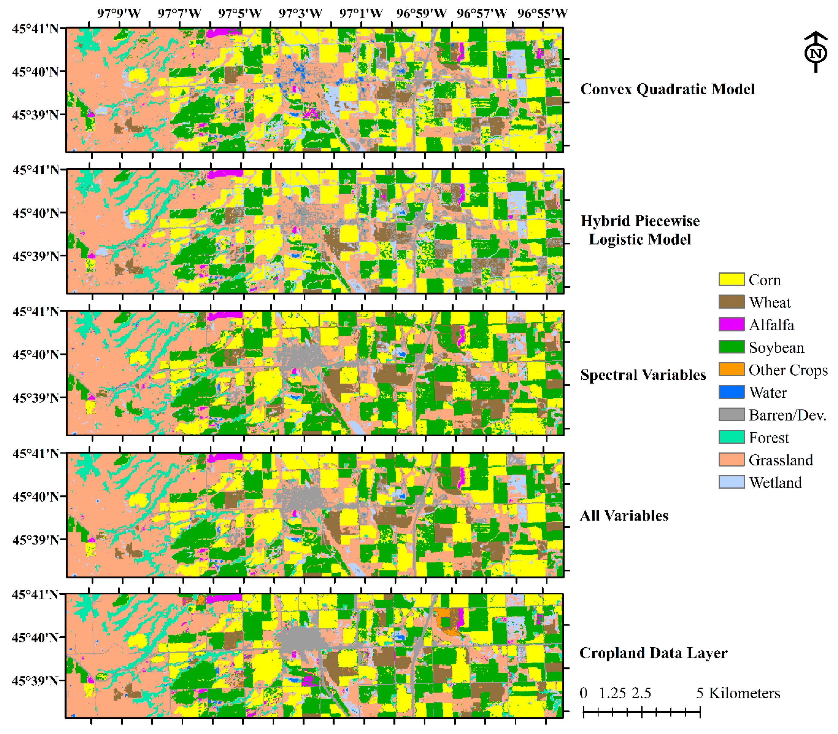
Generally, SPL land cover maps had higher agreement with the CDL than the phenometrically-based maps (Table 12 and Table S16). Similar to model AA, the SPL RFC map clearly improved the accuracy regarding the barren/developed class but was not as accurate as CxQ and HPLM RFC maps when it came to wheat. The land cover map created from CMB RFC models had higher agreement with the CDL than those created with only spectrally-based or phenometrically-based RFC models. Among all ensemble maps, CMB RFC maps were consistently the most accurate. Compared to phenometrically-based and SPL, CMB maps improved PA and UA for both wheat and barren/developed classes. It is also important to note that the barren/developed areas estimated from the phenometrically-based maps were closer to CDL compared to values from the spectrally-based maps. However, both PA and UA of barren/developed from the phenometrically-based maps were lower, thus resulting in fewer correctly assigned pixels (Table 12, Figure 3).
The overall accuracies of ARD maps were greater than those of HLS maps by 1% to 3% (Table 11, Table 12). A possible reason for the lower agreement between HLS and CDL is the difference in projection of the two datasets. While HLS data was produced in the UTM projection for zone 14N using Sentinel’s pixel geometry, both the CDL and ARD data were produced in the AEA projection using Landsat’s pixel geometry. Although CDL and ARD pixels were not perfectly aligned (due to re-projections while creating those products), offsets were only about 3 m in both the latitude and longitude directions. On the other hand, offsets between HLS and CDL data were 15 m in each direction. Re-projection and pixel co-registration to allow pixel-based comparison would negatively affect cross-comparison between the CDL and HLS-based maps more than cross-comparison between the CDL and ARD-based maps. The large offset between HLS and CDL pixels was observed in the kappa indices for location and quantity. Compared to ARD-based maps, HLS-based maps had similar k_Q but lower k_L values, especially in the more accurate maps, i.e., C1S, P25, and CMB (cf. Table 11, Table 12), indicating that the proportional distributions of the two maps were similar, but HLS-based maps had less accurate pixel allocation.

5. Discussion

5.1. Convex Quadratic Versus Hybrid Piecewise Logistic Modeling of LSP for Land Cover Classification

The hybrid piecewise logistic model (HPLM) was first designed to detect vegetation phenology from MODIS time series [34]. The HPLM has a well-refined fitting algorithm, but strict requirements regarding numerical and temporal distributions of observations [22,34]. On the other hand, the convex quadratic model (CxQ) has recently characterized seasonal patterns of vegetated surfaces by incorporating the use of MODIS LST 8-d composites at 1 km spatial resolution [11,46,47]. The fitting algorithm and data requirements for the CxQ are more flexible than for the HPLM, due to fewer parameter coefficients to estimate [18]. When data requirements were satisfied, the HPLM could fit the observed EVI2 pattern more precisely than the CxQ, leading to a higher classification accuracy. However, when fewer observations were available, e.g., outside the Landsat sidelap zones, the CxQ model could serve as a back-up algorithm in this temperate climate where temperatures constrain the initiation and tempo of spring growth. The fundamental challenge for both CxQ and HPLM is dealing with gaps in observations during the growing season, arising from few good observations available in some years and/or over some areas. Although many observations were available for the study area in both years (Figure S4), a lower minimum number of observations (at least ten) was required to fit the HPLM in this study (compared to the fitting for MODIS data in [34] and for AVHRR (Advanced Very High Resolution Radiometer) data in [35]) to generate a map without gaps. Even within the Landsat sidelap zones, we were not always able to retrieve sufficient observations to fit the LSP model [18]. However, the temporal density of observations could be increased by bringing together complementary sensors. For example, our results show that Sentinel-2 data can be used with Landsat ARD in a phenometrically-based classification. An alternative feasible solution may be to leverage very high spatiotemporal but low spectral resolution data from a small satellite constellation to fill any gaps [48].

5.2. Phenometrically-Based Versus Spectrally-Based Classification

Our hypothesis was that phenometrically-based RFC models would be more accurate than the spectrally-based RFC models in vegetated cover types, at least for crops. However, the results showed that the spectrally-based classification yielded slightly higher accuracy metrics (compared to the phenometrically-based classifications) for most classes, including corn and soybean (Table 8). One possible reason for this result is that both spectral and phenometric variables have their own strengths in classification. Compared to spectrally-based RFC models, phenometrically-based RFC models have an advantage of containing the seasonal information or timing of vegetation growth, thus mapping wheat more accurately. However, the phenometrically-based RFC relied on vegetation growth, as represented by the EVI2 time series calculated from the red and NIR bands. On the other hand, spectral variables in spectrally-based RFC models contain far more spectral information from multiple bands and normalized ratios that give the spectrally-based classification an edge in feature separation. The rich information from input variables could help spectrally-based models to perform better for most classes, including some vegetated covers (e.g., corn, soybean, wetland, and grass) (Table 8 and Table S8). Analysis of important variables (Table 9 and Table 10) also helps to explain the better performances of spectrally-based models compared to phenometrically-based models. Both CxQ and HPLM RFC classifications were strongly driven by the maximum fitted EVI2, as shown by the consistent appearance of α as the most important variable in the CxQ RFC models (Table 9) and the appearance of PHHPLM in the top five HPLM RFC models (Table 10). In the study area, all vegetated covers can be classified effectively without seasonal information, except for wheat. A comparison between phenometrically-based and spectrally-based classifications in an area with more complicated cropping patterns (e.g., the wheat-fallow system used in the western Great Plains) might better demonstrate the relative strengths and weakness of these complementary approaches. Nevertheless, the combination of spectral and phenometric variables yielded the most accurate land use/land cover map.

5.3. Impact of Sample Size on Classification Accuracy

Our results confirmed previous findings that larger sample sizes would lead to better classification and a sample size covering 0.25% of the study area would be adequate for a classification study [18,37]. However, in case of data scarcity, smaller sample sizes covering 0.15% and at least 0.05% of the study area might provide acceptable results (cf. Table 5, Tables S7, S14, S15; [41]). Note that RFC models’ accuracy metrics and predicted land cover maps in this study were an ensemble of multiple RFC models. In the case of having a single sample dataset for training and testing, classification may have fairly higher or lower accuracy metrics than the expected value (Figures S1–S3).

5.4. Trade-Offs between Randomness and Accuracy in Sample Dataset

Accuracies of sample pool scenarios in the model AA and the map AA are in opposite orders (Table 5 and Table 11). In model AA, C1S and C2M RFC models performed the worst and the best, respectively. On the other hand, C1S RFC models displayed higher accuracy metrics than C2M RFC models in map AA. To some extent, this result is reasonable. C2M RFC models have higher accuracy metrics in model AA due to more accurate land cover information and higher spatial autocorrelation, but they may have lower predictive power (lower OA in map AA), as some actual characteristics were excluded at the edges. Although it might be necessary to improve the accuracy of the sample datasets to compensate for the low accuracy of some CDL classes and the spatial offsets between HLS, ARD, and CDL data, our results suggest that only minimum corrections (namely, the C1S sample pool) are needed, since there was no improvement in accuracy of the predicted land cover map using sample pools with higher levels of correction.

6. Conclusions

The focus of this study was to evaluate classification accuracy using different sets of input variables derived from either Landsat ARD or HLS time series, including phenometrics generated from two land surface phenology models (CxQ and HPLM), spectral variables, and the combined set of phenometrics and spectral variables. Between the two phenometrically-based classifications, HPLM RFC models exhibited slightly better accuracy but absolute differences in OA were minor (<1%), mostly due to more precise pixel allocation of land cover. Compared to the phenometrically-based RFC models, the spectrally-based RFC models yielded more accurate land cover maps, especially for non-crop cover types. However, the spectrally-based RFC models could not classify wheat accurately. As hypothesized, the most accurate RFC models were retrieved when using both phenometrics and spectral variables as inputs. The combined-variable RFC models overcame weaknesses of both phenometrically-based classifications (low accuracies for non-vegetated covers) and spectrally-based classifications (low accuracies for wheat). The analysis of important variables indicated that classifications of the study area were strongly driven by variables related to the initial green-up phase of seasonal growth and highest EVI2 over the growing season.
We explored land use/land cover classification under different sample pool and sample size scenarios. First, to improve the land cover accuracy of the sample data, both spatial and temporal filters were applied to compensate classification errors of the CDL and offsets between input datasets. The results indicated that a sample pool with a minimum correction of land cover information yielded the most accurate predicted map. Next, land cover classification was also tested with different sample sizes. Although previous findings suggested that a sample size should cover at least 0.25% of the study area to achieve an accurate (OA ≥ 0.90) land cover map, smaller datasets would be acceptable for classification, but should not smaller than 0.05% of the study area, since classification accuracy would decrease rapidly below that threshold.
Land surface phenology modeling requires a substantial number of good quality observations over a year [49]; thus, it may be less suitable for areas with persistent cloud cover if only optical data are available to characterize the LSP. However, the prospect of using phenometrics to enhance land use/land cover classification is very promising. First, our results proved that the use of phenometrics and spectral variables together yielded the most accurate classification and overcame limitations of both phenometrically-based and spectrally-based classifications. Second, seasonality information from all spectral band and ratio time series could be extracted to enhance classification accuracy (e.g., [50]). Finally, the temporal resolution of satellite data can be improved by using comparable sensor datastreams, e.g., Landsat and Sentinel-2, but substantial pre-processing is required to achieve compatibility.
Supplementary Materials

The following are available online at https://www.mdpi.com/2072-4292/11/14/1677/s1.

Author Contributions

Conceptualization: L.H.N and G.M.H.; data curation and analysis: L.H.N; writing—draft: L.H.N and G.M.H.; writing—review and editing: L.H.N and G.M.H.

Funding

This research was supported, in part, by NASA Land Cover Land Use Change program project NNX14AJ32G, the Geospatial Sciences Center of Excellence at South Dakota State University, and the Center for Global Change and Earth Observations at Michigan State University.

Acknowledgments

We would like to thank Xiaoyang Zhang and Jianmin Wang, Geospatial Science Center of Excellence, South Dakota State University, for assistance with the HPLM fitting.

Conflicts of Interest

The authors declare no conflict of interest.

Abbreviations

AAAccuracy Assessment
AEAAlbert Equal Area
AGDDAccumulate Growing Degree-Days
ARDAnalysis Ready Data
CDLCropland Data Layer
CxQConvex Quadratic
DOYDay of Year
ETM+Enhanced Thematic Mapper plus
EVI22-band Enhanced Vegetation Index
HLSHarmonized Landsat Sentinel-2
HPLMHybrid Piecewise Logistic Model
LULCLand Use/Land Cover
LSPLand Surface Phenology
LSTLand Surface Temperature
MODISMODerate resolution Imaging Spectroradiometer
MSIMultiSpectral Instrument
NAD83North American Datum 1983
NASSNational Agricultural Statistics Service
NBARNadir-BRDF Adjusted Reflectance
NDVINormalized Difference Vegetation Index
NLCDNational Land Cover Database
OAOverall Accuracy
OLIOperational Land Imager
PAProducer’s Accuracy
RFCRandom Forest Classifier
SRSurface Reflectance
TMThematic Mapper
UAUser’s Accuracy
USDAUnited States Department of Agriculture
UTMUniversal Transverse Mercator
WGS84World Geodetic System 1984

References

  1. Goebel, J.J. The National Resources Inventory and its Role in US Agriculture; International Statistical Institute: Voorburg, The Netherlands, 1998. [Google Scholar]
  2. Miller, D.; McCarthy, J.; Zakzeski, A. A fresh approach to agricultural statistics: Data mining and remote sensing. In Proceedings of the Joint Statistical Meetings, Washington, DC, USA, 1–6 August 2009; pp. 1–6. [Google Scholar]
  3. Homer, C.; Huang, C.; Yang, L.; Wylie, B.; Coan, M. Development of a 2001 national land-cover database for the United States. ISPRS J. Photogramm. Remote Sens. 2004, 70, 829–840. [Google Scholar] [CrossRef]
  4. Xian, G.; Homer, C.; Fry, J. Updating the 2001 National Land Cover Database land cover classification to 2006 by using Landsat imagery change detection methods. Remote Sens. Environ. 2009, 113, 1133–1147. [Google Scholar] [CrossRef] [Green Version]
  5. Homer, C.; Dewitz, J.; Yang, L.; Jin, S.; Danielson, P.; Xian, G.; Coulston, J.; Herold, N.; Wickham, J.; Megown, K. Completion of the 2011 National Land Cover Database for the conterminous United States–representing a decade of land cover change information. ISPRS J. Photogramm. Remote Sens. 2015, 81, 345–354. [Google Scholar]
  6. Boryan, C. The USDA NASS Cropland Data Layer Program Transition from Research to Operations (2006–2009). White Paper; 2018. Available online: https://www.nass.usda.gov/Research_and_Science/Cropland/SARS1a.php (accessed on 10 March 2019).
  7. Gómez, C.; White, J.C.; Wulder, M.A. Optical remotely sensed time series data for land cover classification: A review. ISPRS J. Photogramm. Remote Sens. 2016, 116, 55–72. [Google Scholar] [CrossRef] [Green Version]
  8. Key, T.; Warner, T.A.; McGraw, J.B.; Fajvan, M.A. A comparison of multispectral and multitemporal information in high spatial resolution imagery for classification of individual tree species in a temperate hardwood forest. Remote Sens. Environ. 2001, 75, 100–112. [Google Scholar] [CrossRef]
  9. Mitchell, J.; Shrestha, R.; Moore-Ellison, C.; Glenn, N. Single and multi-date Landsat classifications of basalt to support soil survey efforts. Remote Sens. 2013, 5, 4857–4876. [Google Scholar] [CrossRef]
  10. Franklin, S.E.; Ahmed, O.S.; Wulder, M.A.; White, J.C.; Hermosilla, T.; Coops, N.C. Large area mapping of annual land cover dynamics using multi-temporal change detection and classification of Landsat time-series data. Can. J. Remote. Sens. 2015, 41, 293–314. [Google Scholar] [CrossRef]
  11. Henebry, G.M.; de Beurs, K.M. Remote sensing of land surface phenology: A prospectus. In Phenology: An Integrative Environmental Science, 2e; Schwartz, M.D., Ed.; Springer: New York, NY, USA, 2013; pp. 385–411. [Google Scholar]
  12. Zhong, L.; Hawkins, T.; Biging, G.; Gong, P. A phenology-based approach to map crop types in the San Joaquin Valley, California. Int. J. Remote Sens. 2011, 32, 7777–7804. [Google Scholar] [CrossRef]
  13. Jia, K.; Liang, S.; Wei, X.; Yao, Y.; Su, Y.; Jiang, B.; Wang, X. Land cover classification of Landsat data with phenological features extracted from time series MODIS NDVI data. Remote Sens. 2014, 6, 11518–11532. [Google Scholar] [CrossRef]
  14. Xue, Z.; Du, P.; Feng, L. Phenology-driven land cover classification and trend analysis based on long-term remote sensing image series. IEEE J. Sel. Top. Appl. Earth Obs. Remote Sens. 2014, 7, 1142–1156. [Google Scholar] [CrossRef]
  15. Yan, E.; Wang, G.; Lin, H.; Xia, C.; Sun, H. Phenology-based classification of vegetation cover types in Northeast China using MODIS NDVI and EVI time series. Int. J. Remote Sens. 2015, 36, 489–512. [Google Scholar] [CrossRef]
  16. Kong, F.; Li, X.; Wang, H.; Xie, D.; Li, X.; Bai, Y. Land cover classification based on fused data from GF-1 and MODIS NDVI time series. Remote Sens. 2016, 8, 741. [Google Scholar] [CrossRef]
  17. Qader, S.H.; Dash, J.; Atkinson, P.M.; Rodriguez-Galiano, V. Classification of vegetation type in Iraq using satellite-based phenological parameters. IEEE J. Sel. Top. Appl. Earth Obs. Remote. Sens. 2016, 9, 414–424. [Google Scholar] [CrossRef]
  18. Nguyen, L.H.; Joshi, D.R.; Clay, D.E.; Henebry, G.M. Characterizing land cover/land use from multiple years of Landsat and MODIS time series: A novel approach using land surface phenology modeling and random forest classifiers. Remote Sens. Environ. 2019. [Google Scholar] [CrossRef]
  19. Tucker, C.J. Red and photographic infrared linear combinations for monitoring vegetation. Remote Sens. Environ. 1979, 8, 127–150. [Google Scholar] [CrossRef] [Green Version]
  20. USGS (U.S. Geological Survey). Landsat collections: U.S. Geological Survey Fact Sheet 2018–3049. 2018. Available online: https://doi.org/10.3133/fs20183049 (accessed on 10 March 2019).
  21. De Beurs, K.M.; Henebry, G.M. Land surface phenology, climatic variation, and institutional change: Analyzing agricultural land cover change in Kazakhstan. Remote Sens. Environ. 2004, 89, 497–509. [Google Scholar] [CrossRef]
  22. Zhang, X. Reconstruction of a complete global time series of daily vegetation index trajectory from long-term AVHRR data. Remote Sens. Environ. 2015, 156, 457–472. [Google Scholar] [CrossRef]
  23. Jiang, Z.; Huete, A.R.; Didan, K.; Miura, T. Development of a two-band enhanced vegetation index without a blue band. Remote Sens. Environ. 2008, 112, 3833–3845. [Google Scholar] [CrossRef]
  24. Congalton, R.G.; Green, K. Assessing the Accuracy of Remotely Sensed Data: Principles and Practices; CRC Press: Boca Raton, FL, USA, 2008. [Google Scholar]
  25. Pontius, R.G., Jr.; Millones, M. Death to Kappa: Birth of quantity disagreement and allocation disagreement for accuracy assessment. Int. J. Remote Sens. 2011, 32, 4407–4429. [Google Scholar] [CrossRef]
  26. Nachar, N. The Mann-Whitney U: A test for assessing whether two independent samples come from the same distribution. Tutor. Quant. Methods Psychol. 2008, 4, 13–20. [Google Scholar] [CrossRef]
  27. Foody, G.M. Classification accuracy comparison: Hypothesis tests and the use of confidence intervals in evaluations of difference, equivalence, and non-inferiority. Remote Sens. Environ. 2009, 113, 1658–1663. [Google Scholar] [CrossRef]
  28. Lakens, D. Equivalence tests: A practical primer for t tests, correlations, and meta-analyses. Soc. Psychol. Personal. Sci. 2017, 8, 355–362. [Google Scholar] [CrossRef] [PubMed]
  29. Dwyer, J.; Roy, D.; Sauer, B.; Jenkerson, C.; Zhang, H.; Lymburner, L. Analysis ready data: Enabling analysis of the Landsat archive. Remote Sens. 2018, 10, 1363. [Google Scholar]
  30. Claverie, M.; Ju, J.; Masek, J.G.; Dungan, J.L.; Vermote, E.F.; Roger, J.C.; Skakun, S.V.; Justice, C. The Harmonized Landsat and Sentinel-2 surface reflectance data set. Remote Sens. Environ. 2018, 219, 145–161. [Google Scholar] [CrossRef]
  31. Wan, Z.; Hook, S.; Hulley, G. MYD11A2 MODIS/Aqua Land Surface Temperature/ Emissivity 8-Day L3 Global 1km SIN Grid V006 [Data Set]; NASA EOSDIS LP DAAC: Sioux Falls, SD, USA, 2015. [Google Scholar] [CrossRef]
  32. Wan, Z.; Hook, S.; Hulley, G. MOD11A2 MODIS/Terra Land Surface Temperature/ Emissivity 8-Day L3 Global 1km SIN Grid V006 [Data Set]; NASA EOSDIS LP DAAC: Sioux Falls, SD, USA, 2015. [Google Scholar] [CrossRef]
  33. Boryan, C.; Yang, Z.; Mueller, R.; Craig, M. Monitoring US agriculture: The US Department of Agriculture, National Agricultural Statistics Service, Cropland Data Layer program. Geocarto Int. 2011, 26, 341–358. [Google Scholar] [CrossRef]
  34. Zhang, X.; Friedl, M.A.; Schaaf, C.B.; Strahler, A.H.; Hodges, J.C.; Gao, F.; Reed, B.C.; Huete, A. Monitoring vegetation phenology using MODIS. Remote Sens. Environ. 2003, 84, 471–475. [Google Scholar] [CrossRef]
  35. Zhang, H.K.; Roy, D.P. Using the 500 m MODIS land cover product to derive a consistent continental scale 30 m Landsat land cover classification. Remote Sens. Environ. 2017, 197, 15–34. [Google Scholar] [CrossRef]
  36. Breiman, L. Random forests. Mach. Learn. 2001, 45, 5–32. [Google Scholar] [CrossRef]
  37. Colditz, R.R. An evaluation of different training sample allocation schemes for discrete and continuous land cover classification using decision tree-based algorithms. Remote Sens. 2015, 7, 9655–9681. [Google Scholar] [CrossRef]
  38. Millard, K.; Richardson, M. On the importance of training data sample selection in random forest image classification: A case study in peatland ecosystem mapping. Remote Sens. 2015, 7, 8489–8515. [Google Scholar] [CrossRef]
  39. Pedregosa, F.; Varoquaux, G.; Gramfort, A.; Michel, V.; Thirion, B.; Grisel, O.; Blondel, M.; Vanderplas, J. Scikit-learn: Machine learning in Python. J. Mach. Learn. Res. 2011, 12, 2825–2830. [Google Scholar]
  40. Gislason, P.O.; Benediktsson, J.A.; Sveinsson, J.R. Random forests for land cover classification. Pattern Recognit Lett. 2006, 27, 294–300. [Google Scholar] [CrossRef]
  41. Rodriguez-Galiano, V.F.; Ghimire, B.; Rogan, J.; Chica-Olmo, M.; Rigol-Sanchez, J.P. An assessment of the effectiveness of a random forest classifier for land-cover classification. ISPRS J. Photogramm. Remote Sens. 2012, 67, 93–104. [Google Scholar] [CrossRef]
  42. Mannel, S.; Price, M.; Hua, D. Impact of reference datasets and autocorrelation on classification accuracy. Int. J. Remote Sens. 2011, 32, 5321–5330. [Google Scholar] [CrossRef]
  43. Deng, C.; Wu, C. The use of single-date MODIS imagery for estimating large-scale urban impervious surface fraction with spectral mixture analysis and machine learning techniques. ISPRS J. Photogramm. Remote Sens. 2013, 86, 100–110. [Google Scholar] [CrossRef]
  44. Du, P.; Samat, A.; Waske, B.; Liu, S.; Li, Z. Random forest and rotation forest for fully polarized SAR image classification using polarimetric and spatial features. ISPRS J. Photogramm. Remote Sens. 2015, 105, 38–53. [Google Scholar] [CrossRef]
  45. Fritz, C.O.; Morris, P.E.; Richler, J.J. Effect size estimates: Current use, calculations, and interpretation. J. Exp. Psychol. Gen. 2012, 141, 2. [Google Scholar] [CrossRef]
  46. Krehbiel, C.; Zhang, X.; Henebry, G.M. Impacts of thermal time on land surface phenology in urban areas. Remote Sens. 2017, 9, 499. [Google Scholar] [CrossRef]
  47. Krehbiel, C.P.; Jackson, T.; Henebry, G.M. Web-enabled Landsat data time series for monitoring urban heat island impacts on land surface phenology. IEEE J. Sel. Top. Appl. Earth Obs. Remote. Sens. 2016, 9, 2043–2050. [Google Scholar] [CrossRef]
  48. Houborg, R.; McCabe, M.F. A cubesat enabled spatio-temporal enhancement method (CESTEM) utilizing Planet, Landsat and MODIS data. Remote Sens. Environ. 2018, 209, 211–226. [Google Scholar] [CrossRef]
  49. Zhang, X.; Wang, J.; Gao, F.; Liu, Y.; Schaaf, C.; Friedl, M.; Yu, Y.; Jayavelu, S.; Gray, J.; Liu, L.; et al. Exploration of scaling effects on coarse resolution land surface phenology. Remote Sens. Environ. 2017, 190, 318–330. [Google Scholar] [CrossRef] [Green Version]
  50. Zhu, Z.; Woodcock, C.E. Continuous change detection and classification of land cover using all available Landsat data. Remote Sens. Environ. 2014, 144, 152–171. [Google Scholar] [CrossRef] [Green Version]
Figure 1. The 2016 reclassified Cropland Data Layer for Roberts County, South Dakota.
Remotesensing 11 01677 g001
Figure 2. Number of good observations for Analysis Ready Data (ARD) and Harmonized Landsat Sentinel-2 (HLS) data in 2016 and 2017.
Remotesensing 11 01677 g002
Figure 3. 2016 ARD-based land cover maps of area around Sisseton, the county seat of Roberts County, South Dakota. Note the barren/developed class in the phenometrically-based RFC maps (CxQ and HPLM) is not as accurate as in the SPL or CMB RFC maps.
Remotesensing 11 01677 g003
Table 1. Variables derived from the Convex Quadratic Model.
ParametersMeaning
α, β, γFitted parameter coefficients of CxQ model (Equation (4))
TTPCxQThermal time to peak (AGDD at the max fitted EVI2) (TTP = –β/2×γ)
PHCxQPeak height EVI2 (max fitted EVI2) (PH = α − β2/4×γ)
HTVHalf-Time Value is value of EVI2 at half-TTP (HTV = α + β×TTP/2 + γ×TTP2/4)
ymaxHighest observed EVI2 value
R2Coefficient of determination of the fitted model
lpos, rposObservation index of start and end of the fitting window
o_allThe total number of “good” observations
o_fitNumber of observations used to fit the CxQ model
o_perRatio between “o_fit” and “o_all”
minx, maxxAGDD at left and right ends of the fitted curve in the first quadrant
peaksNumber of high EVI2 values (≥0.8*ymax) outside the fitting window
jumpsNumber of times that ∆EVI2 ≥ 0.2
Table 2. Variables derived from the Hybrid Piecewise Logistic Model.
ParametersMeaning
gri, vi_griDOY and EVI2 of green-up start
gre, vi_greDOY and EVI 2 of green-up end
grMD, vi_grMDMiddle of gri and gre and its corresponded EVI2
sei, vi_seiDOY and EVI 2 of senescence start
see, vi_seeDOY and EVI 2 of senescence end
se_MD, vi_seMDMiddle of “sei” and “see” and its corresponded EVI2
DPHPLM, PHHPLMDOY with the highest fitted EVI2 and its EVI2
Table 3. Sample pool scenarios.
AcronymProcedure
C1SOnly keep pixels surrounded by 8 of the same neighbors. C1: 1 pixel away from the focal pixel; S: Land cover of a single year.
C1MC1 and matched (M) land cover in 2016 and 2017. M: Only keep pixels with the same CDL class in both 2016 and 2017.
C2SOnly keep pixels surround by 24 of the same neighbors. C2: 2 pixels away from the focal pixel; S: Land cover of a single year.
C2MC2 and matched (M) land cover in 2016 and 2017.
Table 4. Input variables for Random Forest Classifier (RFC) modeling.
NamePractice
CxQUse only the 17 phenometrics from the Convex Quadratic model
HPLMUse only the 14 phenometrics from the Hybrid Piecewise Logistic Model
SPLUse only the 42 spectrally-based variables
CMBUse the combination of 73 variables from CxQ, HPLM, and SPL
Table 5. Overall accuracy (in percent) and kappa indices for location and quantity of 2016 RFC models summarized by sample pools, sample sizes, and input variables. A particular scenario (current row) was compared to a scenario right above it (above row) using the nonparametric Mann–Whitney U test and the TOST equivalence test. The null hypothesis of the U test is that a random accuracy metric of the first scenario (above row) will be less than a random accuracy metric of the second scenario (current row). Significance levels of the U test are indicated by ***, **, and * for p-values of less than 0.001, 0.01, and 0.05, respectively. NS stands for “not significant”. Results of the TOST equivalence test are highlighted in light blue for “not equivalent” and light yellow for “equivalent”. Full pairwise comparisons are provided in Tables S3 and S4.
ScenarioARDHLS
OA k_L k_Q OA k_L k_Q
Sample PoolC1S88.8 0.904 0.917 86.8 0.884 0.906
C1M90.7***0.923***0.926***88.7***0.904***0.914***
C2S90.4NS0.921NS0.924NS89.4***0.909**0.921***
C2M91.8***0.935***0.932***90.7***0.922***0.927***
Sample SizeP0187.1 0.906 0.877 84.8 0.883 0.862
P0590.5***0.919***0.929***89.0***0.903***0.922***
P1591.8***0.927***0.944***90.6***0.914***0.940***
P2592.3***0.931*0.949***91.2***0.919**0.945***
Input SetCxQ86.8 0.879 0.914 86.0 0.871 0.911
HPLM88.6***0.900***0.919NS85.2NS0.867NS0.898NS
SPL92.2***0.943***0.927***91.0***0.928***0.925***
CMB94.1***0.961***0.938***93.4***0.953***0.936***
Table 6. Producer’s and user’s accuracies (in percent) of 2016 RFC models using C1S and C2M sample pools. Significance levels of the U test (C1S < C2M) across rows are indicated by ***, **, and * for p-values of less than 0.001, 0.01, and 0.05, respectively. NS stands for “not significant”. Results of the TOST equivalence tests across rows are highlighted in light blue for “not equivalent” and light yellow for “equivalent”.
Land CoverProducer’s Accuracy (%) User’s Accuracy (%)
ARD HLS ARD HLS
C1SC2M C1SC2M C1SC2M C1SC2M
Corn94.695.7***91.292.6***94.895.9***89.891.5***
Wheat75.478.6***70.274.4***84.490.2***82.089.1***
Alfalfa73.582.6***69.379.9***83.791.2***79.889.6***
Soybean95.496.6***90.392.1***93.695.2***90.492.2***
Other Crops11.250.9***15.355.0***35.870.2***46.671.0***
Water97.498.3***96.298.2***97.597.6***96.396.9***
Barren/Dev.55.160.9***47.456.1***77.079.0***72.475.9***
Forest87.794.0***84.394.5***86.791.1***84.892.4***
Grassland93.094.9***93.696.1***84.988.6***85.690.4***
Wetland66.879.2***73.987.7***74.284.4***76.387.5***
Table 7. Producer’s and user’s accuracies (in percent) of 2016 RFC models using P01 and P25 sample sizes. Significance levels of the U test (P01 < P25) across rows are indicated by ***, **, and * for p-values of less than 0.001, 0.01, and 0.05, respectively. NS stands for “not significant”. Results of the TOST equivalence tests across rows are highlighted in light blue for “not equivalent” and light yellow for “equivalent”.
Land CoverProducer’s Accuracy (%) User’s Accuracy (%)
ARD HLS ARD HLS
P01P25 P01P25 P01P25 P01P25
Corn94.196.2***89.893.6***93.096.7***87.492.6***
Wheat58.187.4***49.685.0***84.590.2NS80.689.0NS
Alfalfa61.987.9***55.086.5***75.292.9NS69.992.0NS
Soybean94.696.8***88.592.8***92.296.1***87.993.6***
Other Crops7.148.3***9.155.9***7.084.7***9.089.5***
Water97.598.5NS97.097.9NS97.497.8NS96.196.8NS
Barren/Dev.49.664.2***38.858.9***72.581.7**66.078.9***
Forest86.693.4NS84.592.8NS85.391.6NS84.791.6NS
Grassland92.694.7***93.795.7***83.788.5***84.890.1***
Wetland64.877.6***74.584.5***72.883.5***74.686.3***
Table 8. PA/UA in percent (%) of 2016 RFC models summarized by sets of input variables. A certain scenario (current column) was compared to a scenario on the left (left column) using nonparametric Mann–Whitney U and TOST equivalence tests. The null hypothesis of the U test is that a random accuracy metric of the first scenario (left column) will be less than a random accuracy metric of the second scenario (current column). Significance levels of the U test are indicated by ***, **, and * for p-values of less than 0.001, 0.01, and 0.05, respectively. NS stands for “not significant”. Results of TOST equivalence tests are highlighted in light blue for “not equivalent” and light yellow for “equivalent”.
MetricsARDHLS
CxQHPLM SPL CMB CxQHPLM SPL CMB
PA_Corn93.093.8***96.0***98.0***89.590.0***93.2***95.6***
PA_Wheat79.375.5NS66.1NS89.1***75.671.8NS60.0NS83.2***
PA_Alfalfa63.687.0***80.8NS84.0***61.185.0***77.6NS79.9***
PA_Soybean93.295.2***97.3***98.5***87.088.4***94.2***95.7***
PA_Other Crops36.234.2NS14.1NS32.6***34.936.7NS31.3NS36.6**
PA_Water94.598.8***99.6***99.5NS93.797.3***99.6***99.5NS
PA_Barren/Dev.40.248.3***73.2***72.6NS37.340.6***64.6***62.5NS
PA_Forest82.889.2***95.9***96.4*80.388.7***95.2***95.5NS
PA_Grassland91.192.5***95.8***96.3***93.792.6NS96.1***97.4***
PA_Wetland68.467.7NS77.5***78.9***84.064.6NS86.0***89.4***
UA_Corn92.094.3***97.1***98.1***86.087.2***94.4***95.6***
UA_Wheat88.488.5*82.1NS92.6***88.584.7NS77.6NS92.3***
UA_Alfalfa79.588.8NS89.4***93.7***78.387.8NS87.5***89.5***
UA_Soybean92.495.4***93.1NS97.2***89.391.4***90.4NS94.8***
UA_Other Crops52.959.3***42.4NS62.7***56.258.4NS59.7***64.3*
UA_Water93.397.7***99.8***99.7NS92.394.3***99.7***99.4NS
UA_Barren/Dev.61.167.1***93.0***92.1NS56.362.1***89.9***88.2NS
UA_Forest83.685.1***93.5***94.5**83.085.2***92.9***94.2***
UA_Grassland83.684.4***89.5***89.5NS88.183.1NS90.2***91.2***
UA_Wetland73.273.2NS84.4***87.5***79.672.6NS86.5***90.1***
Table 9. Top 10 most important variables of CxQ and HPLM RFC models. Variables highlighted in light yellow are those that consistently appear in the top 6 most important variables (at least three times over four-year data combinations). Bolded items are variables related to the initial green-up phase of the seasonal growth.
#CxQ RFC ModelsHPLM RFC Models
2016201720162017
ARDHLSARDHLSARDHLSARDHLS
1ααααgrigrigiMDgiMD
2ββHTVHTVgiMDPHHPLMgregri
3HTVymaxr2minxgrevi_seigrigre
4minxminxminxβPHHPLMgiMDPHHPLMsee
5ymaxHTVβr2vi_grevi_grevi_griPHHPLM
6γPHCxQγγvi_seivi_griseevi_gri
7PHCxQo_fitymaxPHCxQseegreDPHPLMvi_sei
8r2γPHCxQymaxvi_griseevi_seiDPHPLM
9TTPCxQr2o_perTTPCxQseMDseMDvi_seevi_gre
10o_fito_allTTPCxQo_perDPHPLMvi_seMDvi_greseMD
Table 10. Top 10 important variables of SPL and CMB RFC models. In the SPL RFC models, spectral variables in the top 5 that involved SWIR-2 bands are highlighted in light yellow. In the CMB RFC models, spectral variables are highlighted in light blue and phenometrics from the CxQ and HPLM are highlighted in light orange and light green, respectively. Bolded items are variables related to the initial green-up phase of the seasonal growth.
#SPL RFC modelsCMB RFC models
2016201720162017
ARDHLSARDHLSARDHLSARDHLS
1P20_S1P20_BP20_S1P20_BP20_S1αP20_S1α
2P20_S2P80_S2P80_S2P20_S2NgiMDP20_BαgiMD
3P80_S2P80_NP20_S2P80_S2αβP20_S2HTV
4P20_S2RP80_S2GP80_S2GP20_RgriminxHTVminx
5P80_S2GP20_GP20_NP80_S2GP20_S2γminxgre
6P80_NP20_RP50_S2NP20_Nβo_fitgiMDβ
7P20_NP50_NRP20_RP20_GminxHTVgreP20_B
8P20_S2GP50_NBP20_S2NP80_S2RHTVgriβgri
9P80_S2RP80_S2RP50_S2P20_S2RγymaxγP20_R
10P50_NBP20_S2RP20_S2GP50_NRP20_S2RP20_Ggriγ
Table 11. Pixel-based comparison between 2016 predicted land cover maps and CDL, summarized by sample pools and sample sizes.
ScenarioARDHLS
OA%k_Lk_QOA%k_Lk_Q
Sample PoolC1S80.80.8200.87877.90.7820.875
C1M80.40.8190.86877.40.7770.871
C2S80.40.8190.86777.40.7790.866
C2M80.10.8170.86377.00.7800.857
Sample SizeP0178.90.8080.85375.50.7760.828
P0580.10.8170.86677.20.7760.868
P1580.70.8210.87278.00.7830.874
P2581.00.8230.87678.30.7860.876
Table 12. Pixel-wise comparisons between 2016 predicted land cover maps and CDL, summarized by input variables. Land cover area is in km2.
Land CoverInfo.CDLARDHLS
CxQHPLMSPLCMBCxQHPLMSPLCMB
CornArea662674636613641701699615644
UA 83.889.093.393.076.978.688.388.2
PA 85.485.586.590.181.683.182.085.8
WheatArea10386931351218192132107
UA 81.980.048.969.179.675.045.471.9
PA 68.772.564.281.262.667.658.374.7
AlfalfaArea452936333128373433
UA 73.567.266.874.367.261.459.265.9
PA 47.554.548.351.941.749.945.047.9
SoybeanArea746693687780731663646769729
UA 87.291.185.090.783.387.081.286.2
PA 81.083.988.888.974.175.383.784.2
Other CropsArea1311000100
UA 0.061.20.00.00.060.80.00.0
PA 0.04.30.00.00.06.90.00.0
WaterArea154122120126121124125131126
UA 92.894.897.097.589.890.693.494.5
PA 73.274.179.576.972.573.679.677.4
Barren/Dev.Area1316966596081565356
UA 25.529.252.950.619.923.443.539.8
PA 13.514.623.923.112.410.017.517.1
ForestArea644965706841667468
UA 57.256.464.865.658.754.356.460.2
PA 43.257.370.769.636.955.565.163.2
GrasslandArea761872903886916899931917940
UA 74.573.875.774.572.370.572.072.0
PA 85.587.688.289.785.586.486.788.9
WetlandArea262347333239251322286216239
UA 35.935.356.153.140.936.958.154.5
PA 47.544.851.150.850.240.247.949.7
OA 74.676.479.180.871.772.475.577.7
k_L 0.7480.7750.8060.8210.7180.7260.7630.782
k_Q 0.8570.8500.8620.8750.8370.8370.8490.870