Article

Evaluation and Comparison of Random Forest and A-LSTM Networks for Large-scale Winter Wheat Identification

1
State Key Laboratory of Resources and Environmental Information System, Institute of Geographic Sciences and Natural Resources Research, Chinese Academy of Sciences, Beijing 100101, China
2
University of Chinese Academy of Sciences, Beijing 100049, China
3
Henan Polytechnic University, Jiaozuo 454000, China
*
Author to whom correspondence should be addressed.
Remote Sens. 2019, 11(14), 1665; https://doi.org/10.3390/rs11141665
Submission received: 29 May 2019 / Revised: 3 July 2019 / Accepted: 7 July 2019 / Published: 12 July 2019

Abstract

:
Machine learning comprises a group of powerful state-of-the-art techniques for land cover classification and cropland identification. In this paper, we proposed and evaluated two models based on random forest (RF) and attention-based long short-term memory (A-LSTM) networks that can learn directly from the raw surface reflectance of remote sensing (RS) images for large-scale winter wheat identification in Huanghuaihai Region (North-Central China). We used a time series of Moderate Resolution Imaging Spectroradiometer (MODIS) images over one growing season and the corresponding winter wheat distribution map for the experiments. Each training sample was derived from the raw surface reflectance of MODIS time-series images. Both models achieved state-of-the-art performance in identifying winter wheat, and the F1 scores of RF and A-LSTM were 0.72 and 0.71, respectively. We also analyzed the impact of the pixel-mixing effect. Training with pure-mixed-pixel samples (the training set consists of pure and mixed cells and thus retains the original distribution of data) was more precise than training with only pure-pixel samples (the entire pixel area belongs to one class). We also analyzed the variable importance along the temporal series, and the data acquired in March or April contributed more than the data acquired at other times. Both models could predict winter wheat coverage in past years or in other regions with similar winter wheat growing seasons. The experiments in this paper showed the effectiveness and significance of our methods.

Graphical Abstract

1. Introduction

For many years, remote sensing (RS) systems have been widely applied for agricultural monitoring and crop identification [1,2,3,4], and these systems provide many surface reflectance images that can be utilized to derive hidden patterns of vegetation coverage. In crop identification tasks, the information of growing dynamics or sequential relationships derived from time-series images is used to perform classification. Although high-spatial-resolution datasets such as Landsat have clear advantages for capturing the fine spatial details of the land surface, such datasets typically do not have high temporal coverage frequency over large regions and are often badly affected by extensive cloud cover. However, coarse-resolution sensors such as the Moderate Resolution Imaging Spectroradiometer (MODIS) provide data at a near-daily observational coverage frequency and over large areas [5]. While MODIS data are not a proper option for resolving smaller field sizes, they do provide a valuable balance between high temporal frequency and high spatial resolution [6].
Many methods for crop identification or vegetation classification using MODIS time series have been examined and implemented in the academic world [5,6,7]. A common approach for treating multitemporal data is to retrieve temporal features or phonological metrics from vegetation index series obtained by band calculations. According to phenology and simple statistics, several key phenology metrics, such as the base level, maximum level, amplitude, start date of the season, end date of the season, and length of the season, extracted from time-series RS images are used as classification features that are sufficient for accurate crop identification. For example, Cornelius Senf et al. [5] mapped rubber plantations and natural forests in Xishuangbanna (Southwest China) using multispectral phenological metrics from MODIS time series, which achieved an overall accuracy of 0.735. They showed that the key phenological metrics discriminating rubber plantations and natural forests were the timing of seasonal events in the shortwaved infrared (SWIR) reflectance time series and the Enhanced Vegetation Index (EVI) or SWIR reflectance during the dry season. Pittman et al. [6] estimated the global cropland extent and used the normalized difference vegetation index (NDVI) and thermal data to depict cropland phenology over the study period. Subpixel training datasets were used to generate a set of global classification tree models using a bagging methodology, resulting in a global per-pixel cropland probability layer. Tuanmu et al. [7] used phenology metrics generated from MODIS time series to characterize the phenological features of forests with understory bamboo. Using maximum entropy modeling together with these phenology metrics, they successfully mapped the spatial distribution of understory bamboo. To address image noise such as pseudo-lows and pseudo-hikes caused by shadows, clouds, weather or sensors, many studies have used mathematical functions or complex models to smooth the vegetation index time series before feature extraction. Toshihiro Sakamoto et al. [8] adopted wavelet and Fourier transforms for filtering time-series EVI data. Zhang et al. [9] used a series of piecewise logistic functions fit to remotely sensed vegetation index data to represent intra-annual vegetation dynamics. Furthermore, weighted linear regression [10], asymmetric Gaussian smoothing [11,12], Whittaker smoothing [13], and Savitzky-Golay filtering [14] have also been widely used for the same reason. Yang Shao et al. [15] compared the Savitzky-Golay, asymmetric Gaussian, double-logistic, Whittaker, and discrete Fourier transformation smoothing algorithms (noise reduction) and applied them to MODIS NDVI time-series data to provide continuous phenology data for land cover classifications across the Laurentian Great Lakes Basin, proving that the application of a smoothing algorithm significantly reduced image noise compared to the raw data.
Although temporal feature extraction-based approaches have exhibited good performance in crop identification tasks, they have some weaknesses. First, general temporal features or phenological characteristics may not be appropriate for the specific task. Expert experience and domain knowledge are highly needed to design proper features and a feature extraction pipeline. Second, the features extracted from the time series cannot always fully utilize all the data, and information loss is inevitable. These types of feature extraction processes usually come with limitations in terms of automation and flexibility when considering large-scale classification tasks [16].
Intelligent algorithms such as random forest (RF) and deep neural networks (DNNs) can learn directly from the original values of MODIS data. They can apply all the values of a time series as input and do not need well-designed feature extractors, which could prevent the information loss that often occurs in temporal feature extraction. These algorithms are convenient for large-scale implementation and application, and there are many processing frameworks based on RF or DNNs that are being implemented for cropland identification. Related works will be introduced in the next paragraphs.
Recently, RF classifiers have been widely used for RS images due to their explicit and explainable decision-making process, and these classifiers are easily implemented in a parallel structure for computing acceleration. Rodriguez-Galiano et al. [17] explored the performance of an RF classifier in classifying 14 different land categories in the south of Spain. Results show that the RF algorithm yields accurate land cover classifications and is robust to the reduction of the training set size and noise compared to the classification trees. Charlotte Pelletier et al. [18] assessed the robustness of using RF to map land cover and compared the algorithm with a support vector machine (SVM) algorithm. RF achieved an overall accuracy of 0.833, while SVM achieved an accuracy of 0.771. Works based on RF usually use a set of decision trees trained by different subsets of samples to make predictions collaboratively [19]. However, the splitting nodes still used well-designed features with random selection, and this procedure might be complex and inefficient for the classification of large-scale areas. In this paper, we proposed an RF-based model that directly learns from the original values of the MODIS time series for large-scale crop identification in the Huanghuaihai Region to address the task in an efficient manner.
Considering the successful applications of deep learning (DL) in computer vision, deep models have also been evaluated for time-series image classification [16,20,21]. Researchers usually use pretrained baseline architectures of convolutional neural networks (CNNs), such as AlexNet [22], GoogLeNet [23] and ResNet [24], and fine-tuning to automatically obtain advanced representations of data, which are usually followed by a softmax layer or SVM to adapt to specific RS classification tasks. For times series scenarios, recurrent neural networks (RNNs) and long short-term memory (LSTM) networks are often used to analyze RS images due to their ability to capture long-term dependencies. Marc Rußwurm et al. [20] employed LSTM networks to extract temporal characteristics from a sequence of SENTINEL 2A observations and compared the performance with SVM baseline architectures. Zhong et al. [16] designed two types of DNN models for multitemporal crop classification: one was based on LSTM networks, and the other was based on one-dimensional convolutional (Conv1D) layers. Three widely used classifiers were also tested and compared, including gradient boosting machine (XGBoost), RF, and SVM classifiers. Although LSTM is widely used for sequential data representation, Zhong et al. [16] revealed that its accuracy was the lowest among all the classifiers. Considering that the identification of crop types is highly dependent on a few temporal images of key growth stages such as the green-returning and jointing stages of winter wheat, it is important for the model to have the ability to pay attention to the critical images of the times series. In early studies, attention-based LSTM models were used to address sequence-to-sequence language translation tasks [25], which could generate a proper word each time according to the specific input word and the context. Inspired by the machine translation community and crop growth cycle intuition, we proposed an attention-based LSTM model (A-LSTM) to identify winter wheat areas. The LSTM part of the model transforms original values to advanced representations and then follows an attention layer that encodes the sequence to one fixed-length vector that is used to decode the output at each timestep. A final softmax layer is then used to make a prediction.
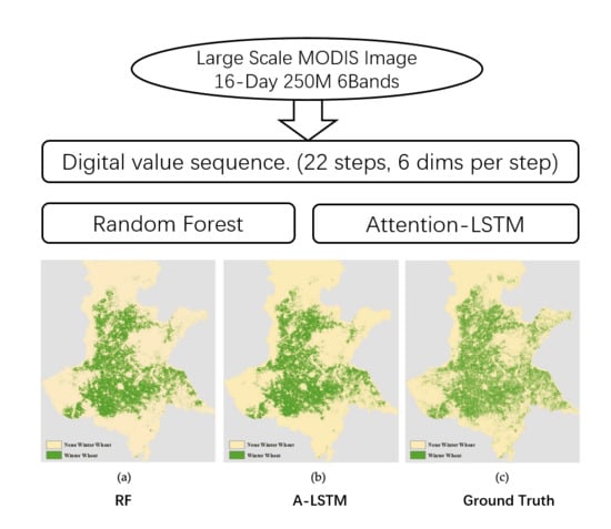
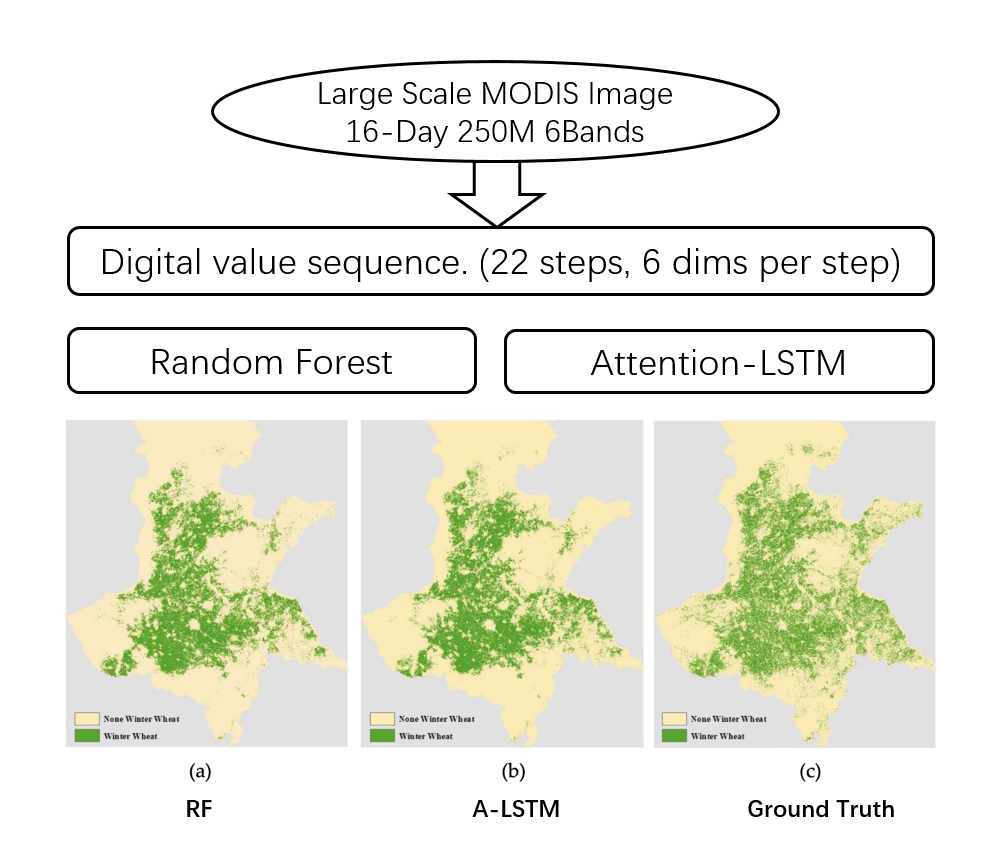
In this study, we proposed two models, RF and A-LSTM, that can be efficiently used for large-scale winter wheat identification throughout the Huanghuaihai Region, by building an automatic data preprocessing pipeline that transforms time-series MODIS tiles into training samples that can be directly fed into the models. As this study is the first to apply an attention mechanism-based LSTM model to the classification of time-series images, a comparison with RF and an evaluation of the performance were also conducted. In addition, we analyzed the impacts of the pixel-mixing effect with two different training strategies in this paper. Furthermore, with the intuition that there is some difference in wheat sowing and harvesting time from north to south, we also evaluated the generalizability of the models to different areas. Finally, our models were used to identify the distribution of winter wheat over the past year, and we evaluated the performance via visual interpretation. Finally, we discussed the advantages and disadvantages of our models.

2. Materials

2.1. Study Area

The Huanghuaihai Region, located in the north-central region of China, surrounds the capital city of Beijing, which is shown in Figure 1. It consists of seven provinces or municipality cities (i.e., Beijing, Tianjin, Hebei, Shandong, Henan, Anhui, and Jiangsu) stretching over an area of 778.9 thousand square kilometers. Most of the Huanghuaihai Region lies within the North China Plain, which is formed by deposits from the Yellow River, Huai River, Hai River and their hundreds of branches. This region is bordered to the north by the Yanshan Mountains, to the west by the Taihang Mountains, to the south by the Dabie Mountains and the Yangtze River, and to the east by the East China Sea [26]. This region has a typical continental temperate and monsoonal climate with four distinct seasons, including cold and dry winters and hot and humid summers. The Huanghuaihai Region is one of the most important agricultural granaries in China, and the chief cereal crops include winter wheat, corn, millet, and potatoes. Winter wheat is usually planted from September to October and harvested in late May or June of the following year. Winter wheat is highly dependent on the water conditions, and artificial irrigation is supplied in this area [27].

2.2. Materials Description

2.2.1. MODIS Data

In this section, we described the time-series images and reference data used for winter wheat identification in our paper. We downloaded 110 MODIS product images, specifically the MODIS/Terra vegetation indices 16-Day L3 Global 250-m SIN Grid (MOD13Q1, Collection 6), from NASA Level-1 and Atmosphere Archive & Distribution System Distributed Active Archive Center (LAADS DAAC). The product has four reflectance bands, i.e., blue, red, near-infrared and middle-infrared, which are centered at 469 nm, 645 nm, 858 nm, and 3.5 µm, respectively, and two vegetation index bands, NDVI and EVI, which can be used to maintain sensitivity over dense vegetation conditions [28]. The two vegetation indices, NDVI and EVI, are computed from atmospherically corrected bidirectional surface reflectance data that are masked for water, clouds, heavy aerosols, and cloud shadows. Specifically, the NDVI is computed from the near-infrared and red reflectance, while the EVI is computed from near-infrared, red, and blue reflectance. The detailed equations are as follows:
N D V I = ρ N I R ρ R e d ρ N I R + ρ R e d
E V I = ρ N I R ρ R e d 1 + ρ N I R + 6 × ρ N I R 7.5 × ρ B l u e
where ρ NIR , ρ Red and ρ Blue represent near-infrared, red and blue reflectance, respectively. Global MOD13Q1 data are provided every 16 days at a 250-m spatial resolution as a gridded level-3 product in the sinusoidal projection. Cloud-free global coverage is achieved by replacing clouds with the historical MODIS time-series climatology record. Vegetation indices are used for global monitoring of vegetation conditions and in products that exhibit land cover and land cover changes. The 110 images downloaded in this study span the period from October 2017 to July 2018 with a 16-day interval, resulting in 22 timesteps. Each timestep contains five tiles that can entirely cover the Huanghuaihai Region. We selected all six bands of each tile in the experiments, and the models could fully capture the reflectance information, which would be effective for crop identification.
To evaluate the generalizability of the models on historical data, we collected the same MOD13Q1 product data for the 2016–2017 growing season for additional experiments.

2.2.2. Reference Data

It is very challenging to collect reference data. Fortunately, we acquired a crop map of the winter wheat distribution for the 2017–2018 growing season in the Huanghuaihai Region from the Chinese Academy of Agricultural Sciences. The wheat map has a spatial resolution of 16 m and is in the Albers equal-area conic projection. Each pixel in the map is assigned a value of 0 or 1, which represent winter wheat or no winter wheat growth. Since we were not provided any details regarding how the map was completed or the reliability of the data, we simply reassessed the map by manually collecting samples. Specifically, we randomly selected 1000 pixels in the map and interpreted the pixels visually based on images acquired from the Planet Explorer API (https://www.planet.com/explorer/). We acquired two high-resolution images in March 2018 and June 2018 from the Planet Explorer API, which are shown in Figure 2. First, it is easy to distinguish non-vegetation areas such as water, residential areas and bare land using images acquired in the two stages via visual interpretation. Practically, most vegetation in the Huanghuaihai Region is a deciduous forest, which is gray and still not germinated in March, while winter wheat has entered the green-returning stage. The few evergreen forests, such as pines and cypresses, will not turn yellow like mature wheat in June. To the best of our knowledge, the main crop during the period from October 2017 to June 2018 was winter wheat, and there were no other crops or vegetation with growing stages similar to those of winter wheat in March and June. According to the images acquired from the two critical growing periods of winter wheat, a pixel was assumed to be winter wheat when it appeared green in March and yellow in June. The evaluation results show that the overall accuracy of the crop map is 0.95, the precision of winter wheat is 0.89, the recall of winter wheat is 0.83 and the F1 score is 0.86 (The detailed explanations of overall accuracy, precision, recall and F1 score are shown in Section 4.3).
Similarly, we visually interpreted 1000 pixels at the same locations during the 2016–2017 growing season from the Planet Explorer API in the same manner to form our historical testing dataset. These collected samples were used to evaluate the accuracy of the prediction map informed by the trained models using historical (2016–2017) MODIS data.

2.3. Data Preprocessing

In this study, we built a data preprocessing pipeline to extract training samples from the MODIS time series. First, image mosaics were applied to the five image tiles at each timestep. Then, mosaic images were projected to the Albers equal-area conic coordinate system, which was coincident with the reference data, thus stably maintained the area of each cell. Next, a mask of the Huanghuaihai Region was used to extract the data within the study boundary. Since the spatial resolution of MODIS data was 250 m, we resampled the 250-m-spatial-resolution MODIS data to a spatial resolution of 224 m with the nearest neighbor resampling method and aligned them with the reference data, which have a 16-m spatial resolution. Therefore, 196 pixels of the reference map were aligned using a 0-1 annotation within a single MODIS cell. Furthermore, we counted the quantities of 0s and 1s in each MODIS cell, which were used to distinguish pure cells that were completely filled with 0 or 1 values from mixed cells that were filled with both 0 and 1 values. Some crop map pixels within the MODIS cells inside the border had no values, and we simply removed these incomplete data. To extract training samples, each pure MODIS cell was annotated with 0 or 1, which represented winter wheat or no winter wheat growth, respectively. For mixed MODIS cells, a threshold was selected to determine whether the cell should be labeled as positive or negative, and these cells were labeled as 1 _ (mixed pixel wheat) or 0 _ (mixed pixel no-wheat). The following inequality shows the labeling process.
y = { 1 ,     ( c = 196 ) 1 _ ,     ( c θ ) 0 _ ,     ( c < θ ) 0 ,     ( c = 0 )
where y denotes the label of a MODIS cell, c denotes the quantities of wheat pixels of reference map within one MODIS cell, and θ is the threshold which is used to determine the label of mixed MODIS cell. We simply set θ to 98. As mentioned in Section 2.2.1, each timestep of a MODIS image has 6 bands, which are blue, red, near-infrared, middle-infrared, NDVI and EVI. We took the digital value from each MODIS cell throughout the 22 timesteps and the corresponding labels as the training samples; each sample has 132 variables and one class annotation. Throughout the Huanghuaihai Region, we acquired approximately 13 million samples, and the distribution of samples is shown in Table 1.

2.4. Dataset Partition

To train and evaluate our model, the datasets must be partitioned into training sets and testing sets. As the MODIS data have a cell size of 250 m, the spatial correlation might be nonsignificant. We assume that each MODIS cell is independent of the others. The total dataset was partitioned in the following manner:
  • Pure-mixed pixel set. The entire dataset was first randomly partitioned into a training set and testing set with a ratio of 4:1. Both the training set and testing set consist of pure-pixel samples and mixed-pixel samples. We call this type of training set a pure-mixed pixel set.
  • Pure pixel set. Then, we further selected all the pure-pixel samples (the entire MODIS cell is either covered with winter wheat or there is no winter wheat) from the pure-mixed pixel set as the new training dataset, which was called the pure pixel set, with the intuition that pure-pixel samples might be representative of the characteristics of wheat areas, while mixed-pixel samples might include noise. We kept the testing dataset unchanged but trained models using the pure-mixed pixel set and pure pixel set for further studies.

2.5. North-South Partition

To evaluate the generalizability of our model to different areas, we also divided our dataset into several parts according to the pixel location from north to south and utilized three parts for training and the rest parts for testing. As shown in Figure 3, the dataset was equally partitioned into eight parts according to latitude. The number of samples in each part is reported in Table 2. As the numbers of samples in Part 1 and Part 2 were small, we combined part 1, part 2 and part 3 to form the training set and testing set with the ratio of 4:1, and used part 4, part 5, part 6, part 7 and part 8 to evaluate the generalizability.

3. Methods

3.1. RF Method for Crop Identification

The RF method is an ensemble learning algorithm that consists of many decision trees that are combined to create a prediction. Each tree in the ensemble is trained using a bootstrap sampling strategy (sample drawn with replacement), in which the training dataset of an individual tree is a subset randomly picked from the whole dataset [19]. In addition, when splitting a node during the construction of the tree, the split point that is chosen is the best split among a random subset of the features. The final output is the average of all the trees, thus decreasing the variance of the results. Although the bias of the forest usually increases slightly due to the randomness in the tree, this increase is less than the increase in bias required to compensate for the decrease in variance. As a result, the method performs better.
As shown in Section 2.2.1, our datasets are composed of 22 timesteps, and each timestep includes four raw reflectance bands and two vegetation index bands; thus, each sample contains 132 variables with an annotated label. RF operates by constructing multiple random classification trees, and each tree randomly selects several variables to make decision rules. In our experiment, n and k denote the number of trees and the number of selected variables, respectively. The number of trees n represents the complexity and ability of RF to learn patterns from the data. Therefore, n needs to be large enough in case some samples or variables are selected only once or even missed in all subspaces. As n increases, the performance of RF tends to remain unchanged, however, the computing resource needs to increase. An increase in the selected variables k generally improves the performance of an individual tree, but the variance of an individual tree decreases, and the computing resources required for the individual tree increase. Hence, we need to strike a balance and find the two optimal parameters n and k . To do so, we built many RF models with n increasing from 100 to 1000 and k increasing from 2 to 132. The overall accuracy was used to evaluate the performance of the model. In addition, the minimum number of samples required to split a node was set to 2, while the minimum number of samples of a leaf node was set to 1. The maximum tree depth was not fixed, and the nodes were expanded until all leaves were pure or until all leaves contained less than the minimum number of samples. For each individual tree, Gini impurity was used to measure the quality of a split. When making an inference, RF combines all the equally weighted tree classifiers by averaging their probabilistic predictions instead of letting each classifier vote for a single class. The predicted class is the one with the highest probability.

3.2. A-LSTM Architecture for Crop Identification

LSTM is a kind of special RNN architecture that is designed for long-term dependency problems. Both the standard RNN and LSTM have repeated neural units that can be thought of multiple copies of the same network and have the form of a chain of repeating modules in a neural network. In standard RNNs, the repeating module will have a very simple structure, such as a single tanh layer, as shown in Figure 4. LSTMs also utilize this chain structure, but the repeating module has a different structure. Instead of having a single neural network layer, there are four gates, which are the forget gate, input gate, modulation gate, and output gate, as shown in Equation (4)–(7), respectively, and these gates interact in a specific manner [20].
f t = σ f ( W d a t a f x t + W s t a t e f h t 1 + b f ) ,
i t = σ i ( W d a t a i x t + W s t a t e i h t 1 + b i ) ,
g t = σ g ( W d a t a g g t + W s t a t e g h t 1 + b g ) ,
o t = σ o ( W d a t a o x t + W s t a t e o h t 1 + b o ) ,
These gates influence the ability of LSTM cells to discard old information, gain new information and use that information to create an output vector. The cell state vector c t stores the internal memory and is then updated using the Hadamard operator ⊙, which performs elementwise multiplication, while the layerwise hidden state vector is further derived from the LSTM output gate vector o t [20].
c t = f t c t 1 + i t g t ,
h t = o t σ h ( c t ) ,
To address the original crop identification problem with time-series MODIS images, we proposed an end-to-end encoder-decoder architecture, which is shown in Figure 5. The encoder consists of three bidirectional LSTM layers that are stacked together with the full sequence returned. The input sequence x , which is shown in Equation (10), has 22 timesteps and six variables in each step, which is coincident with our time-series data:
x = ( x 1 , , x i , , x t ) , x i R k
where t is the length of input sequence and k is the dimensionality of data.
In the encoder, each LSTM layer has 128 hidden units and returns the full sequence to the next layer. The output of the three-layer encoder, which is shown in Equation (11), is a sequence of hidden states:
h = ( h 1 , , h i , , h t ) , h i R k
h i = f ( x i , h i 1 )
where h i represents the hidden state at time i and f is a nonlinear function.
In the decoder section, considering that it is difficult for the network to address long sequences, we included an attention mechanism in our network [25]. This mechanism looks at the complete encoded sequence to determine which encoded steps to weight highly and generates a context vector c j for each class. Each encoded step h i includes the information of the whole input sequence due to the recurrent layers, and it has a strong focus on the parts surrounding the i-th step of the input sequence. The context vector c j is computed by the weighted sum of these annotations h i :
c j = i = 1 t α j i h i
where the weight α j i for each h i is computed by
α j i = e x p ( e j i ) i = 1 t e x p ( e j i )
where t is the length of the encoded sequence and e j i is an alignment model, which is shown Equation (15), represents how well the output at position j and the hidden annotation h i match.
e j i = g ( s j , h i )
y = softmax ( s )
where s j is the hidden neuron of the output at position j and y represents the probability distribution of wheat and no-wheat.

3.3. Comparison and Evaluation of the Model Performance

In this paper, we used four metrics to evaluate the performance in the context of the binary classification problem. The precision, recall, overall accuracy, and F1 score were derived from the confusion matrix charted by the predicted and actual classification results [29]. The confusion matrix is shown in Table 3. In the table, positive and negative represent winter wheat and no-wheat, respectively. TP and FP refer to the number of predicted positives that were correct and incorrect, and TN and FN refer to the number of predicted negatives that were correct and incorrect. The four metrics are defined in Equations (17)–(20), respectively. Specifically, the precision denotes the proportion of predicted positives that are actual positives, while the recall denotes the proportion of actual positives that are correctly predicted positives. The overall accuracy is the proportion of the total cases that are correctly predicted, while the F1 score represents the harmonic mean of the recall and precision.
p r e c i s i o n = T P T P + F P
r e c a l l = T P T P + F N
o v e r a l l a c c u r a c y = T P + T N T P + F P + F N + T N
f 1 s c o r e = 2 × p r e c i s i o n × r e c a l l p r e c i s i o n + r e c a l l
First, the two models were trained with the pure-mixed pixel set consisting of pure pixel samples and mixed pixel samples. Considering that pure-pixel samples are representative of the characteristics of wheat areas, while mixed-pixel samples might include noises, we also used the pure pixel set to train the two models. We kept the testing set unchanged to evaluate the performances of the two models trained with the two different datasets. Moreover, we evaluated the generalizability of the models via the north-south dataset partitioning strategy. In practice, our models could also be used to identify croplands in historical datasets. Field-collected reference data were used for analysis and evaluation. More details about the experimental results and analysis are provided in the next section.

4. Experiments and Results Analysis

4.1. RF Fine-Tuning

We used the Python Scikit-learn [30] package to implement our RF experiments following the instructions in Section 3.1. Hundreds of RF models were built to fine-tune the RF parameters n (number of trees) and k (number of selected variables) with different combinations, which are shown in Figure 6. We used the overall accuracy score to measure the performance of each model. To balance performance and the cost of computation, the parameter combination with the highest score was chosen. Figure 6 shows the changes in model performance with n values from 100 to 1000 and k values from 2 to 132. When n equals 500 and k equals 40, the performance of the RF method remains stable; thus, we selected this combination for the following experiments.

4.2. A-LSTM Training and Evaluation

For the A-LSTM method, we used Python TensorFlow [31] and the Keras [32] package to implement our model. The cross-entropy loss was calculated, and the RMSprop (Root Mean Square Prop) algorithm was used to optimize the model [33]. During training, we used the mini-batch strategy and set the batch size to 128. We used an NVIDIA TESLA V100 graphics card to train the model, and after 500 epochs (an epoch is an iteration over the entire dataset), the model converged to the global optimum. Figure 7 shows the training procedure and validation results with each step iteration. Finally, our LSTM model achieved an overall accuracy score of 0.85 on the pure-mixed pixel set and 0.82 on the pure pixel set. We will discuss the performance thoroughly below.

4.3. Identification Metrics

The overall accuracy of the RF trained on the pure-mixed pixel set was 0.87 (±0.01), and the overall accuracy of the RF trained on the pure pixel set was 0.85 (±0.01), while the overall accuracies of the A-LSTM trained on these two datasets were 0.85 (±0.01) and 0.82 (±0.01), respectively. The overall accuracy scores were high because the no-wheat class accounts for approximately 85 percent of the dataset. Thus, the accuracy scores were dominated by the majority class. However, the F1 score is the weighted average of the precision and recall, which is a better metric for such an uneven dataset. Specifically, the F1 scores of RF and A-LSTM trained on the pure-mixed pixel set were 0.72 and 0.71, while the scores of the two models trained on the pure pixel set were 0.68 and 0.66. More details regarding the performance score are shown in Table 4.
In general, the two models behaved better when they were trained on the pure-mixed pixel set. For comparison, when the pure pixel set was utilized, the precision of the two models improved, while the recall worsened. In total, the two models trained with the pure-mixed pixel set were more stable, traded precision for recall and achieved high F1 scores and overall accuracy, which are highly recommended in practical applications. This result occurred because the data distribution of the test dataset was the same as that of the pure-mixed pixel set. This phenomenon might cause severe overfitting problems when the models are trained on only pure-pixel samples. In some classification cases that require large amounts of manually collected training data, whether the selected samples include mixed pixels needs to be reconsidered, and the impact of including these cells needs to be evaluated.
The classified wheat map resulting from the RF and A-LSTM models trained with the pure-mixed set is shown in Figure 8a,b, while the reference wheat map is shown in Figure 8c. The numbers of wheat pixels in the three maps were 3296256, 3327509, and 3269754. According to the map, most of the crop areas were correctly predicted in the plain area, while there were extensive differences between the prediction and reference data in the border between wheat areas and no-wheat areas or some isolated wheat areas. Thus, the many mixed cells that might include crops, buildings, and mountains result in irregular spectral reflectance. In addition, although the numbers of wheat pixels in the prediction map and reference map were similar, there was a slight visual difference. In Figure 9a,b, wheat pixels are more likely to be clustered together, while there are many isolated wheat areas in the reference map. Generally, wheat areas among continuous no-wheat areas or no-wheat areas among continuous wheat areas were very likely to be misclassified.

4.4. Feature Importance

The relative depth of a feature used as a decision node in a tree can be used to assess the relative importance of that feature with respect to the predictability of the target variable. Features used at the top of the tree contribute to the final prediction of a large fraction of the input samples. The expected fraction of samples that these features contribute to can thus be used as an estimate of the relative importance of the features. In the Scikit-learn package, the fraction of samples a feature contributes to is combined with the decrease in impurity from splitting them to create a normalized estimate of the predictive power of that feature. By averaging the estimates of predictive ability over several randomized trees, one can reduce the variance in such an estimate and use it for feature selection. This process is known as the mean decrease in impurity [30].
In this paper, we visualized the feature importance of 132 variables in RF, which is shown in Figure 9a. The importance scores were the mean scores of all individual trees. The top 10 variables are shown in Table 5; these variables are 2018081_EVI, 2018081_NDVI, 2018097_EVI, 2018081_NIR, 2018097_NIR, 2018161_NDVI, 2018097_NDVI, 2018113_EVI, 2018065_EVI and 2018245_NDVI, where the first part of each variable represents the day of the year, and the last part represents the band. Furthermore, we summed six importance scores per timestep and 22 importance scores per band, which are shown in Figure 9b,c. Generally, variables in March or April 2018 were more important than others. Moreover, EVI and NDVI had higher importance scores than raw reflectance bands.
The differences of feature importance among variables could be explained by several points. According to the typical growing cycles of winter wheat, wheat enters the green-returning stage in late February or early March, while most other vegetation in the Huanghuaihai Region is deciduous forest, which is gray and still not germinated; this phenomenon leads to a higher importance of data captured in March or April, such as 2018081_EVI, 2018081_NDVI, 2018097_EVI. For the comparison between vegetation index bands and spectral reflectance bands, vegetation indices are more sensitive over dense vegetation conditions and have high importance scores.
For the A-LSTM model, the context vector c j of output class j determines which encoded steps to weigh highly and is calculated as the weighted sum of these encoded steps. As shown in Section 3.2, the weight α ji can be considered the probability that the j-th class is aligned to the i-th step of the encoded sequence. Since different samples have different weight distributions and the weight distribution of a single sample is usually noisy or not sufficiently representative of the alignment pattern, we simply used the mean of the weight distribution of the whole test dataset for visualization. As shown in Figure 10, the two curves represent the weight distribution along the encoded sequence for the two classes, and the integral of each curve is equal to 1. According to the figure, the wheat class is highly aligned with the 16th step of the encoded sequence, which was acquired in April 2018 (the 113th day of the year 2018). Thus, there is a very high probability that the wheat class is aligned with the 16th step of the encoded sequence, which contains all the information of the input sequence, with a strong focus on the parts surrounding the 16th step of the input sequence. Compared to the variable importance scores of RF, they both show that sequence data acquired in April are more important for the winter wheat identification problem using time-series data.

4.5. Generalizability in Different Areas

To evaluate the generalizability in different areas, we divided the entire dataset into eight parts from north to south, the details of which are presented in Section 2.5. The evaluation results are reported in Table 6. None of the precision, recall, and accuracy metrics exhibited significant patterns except for the F1 score. Specifically, the F1 score of the RF model decreased as the evaluation dataset moved away from the training set. Since the F1 score represents the harmonic mean of the recall and precision, it is appropriate to use it to represent the generalizability of the model. According to the experiments, the model achieved the best performance when the testing set and training set were in the same part, because they had the same data distribution. When the trained model was required to perform prediction in other areas, the performance worsened. The main reason for this difference is that the winter wheat growing season in the Huanghuaihai Region changes slightly from north to south. We divided the growing season into six growth stages: sowing, overwintering, green-returning, jointing, flowering, and maturation. The maps of the starting times of the six growth stages are shown in Figure 11. Each raster pixel represents the day of the year when winter wheat entered the corresponding stage. The first two maps show the growing times in 2017, and the other maps show the growing times in 2018. Contour lines are also shown on the maps. The six raster maps were interpolated from data recorded from 82 agricultural stations distributed in the Huanghuaihai Region. The time interval of the same growing stage from south to north was 30 or 40 days at most. Therefore, to obtain the best model performance, the growing season in the predicting area must be as close as possible to that of the training area, and a new model should be retrained in the prediction area for practical applications if necessary.

4.6. Inference on Historical Data

To determine the historical winter wheat distribution, we also applied the two models to historical MODIS data from the Huanghuaihai Region. Specifically, we collected time-series data for the 2016–2017 growing season, which were processed by the same data preprocessing pipeline. Using the two models trained on Pure-mixed pixel set, which is described in Section 2.4, we obtained two historical winter wheat distribution maps of the Huanghuaihai Region, which are shown in Figure 12a,b. To evaluate the accuracy of the two prediction maps, we randomly selected 1000 cells from the Huanghuaihai Region and interpreted them visually via the Planet Explorer API, which was introduced in Section 2.2.2. The distribution of the 1000 cells is shown in Figure 12c. Similarly, we used the annotation strategy described in Section 2.2.2. Then, two confusion matrices with the predicted and reference samples were generated. They are reported in Table 7 and Table 8, respectively. For the winter wheat class, the recall, precision and F1 score predicted by the RF model were 0.720, 0.739 and 0.729, while these values for the A-LSTM model were 0.703, 0.741 and 0.721, respectively. Generally, the two models achieved comparative performance in the 2016–2017 growing season, which proved our concept.

5. Discussion

Our two models achieved F1 scores of 0.72 and 0.71 for identifying the winter wheat distribution in the Huanghuaihai Region. Previous works such as Senf et al. [5], Tuanmu et al. [7], Rodriguez-Galiano et al. [17], Charlotte Pelletier et al. [18], and Marc Rußwurm et al. [20] regarding land cover classification or crop identification usually focused on only a small area, such as a county or city, which resulted in a classification map that was more detailed than ours. However, our trained models could also easily recognize the approximate winter wheat distribution, but in a large-scale area, and these models could be especially used in some close areas or historical cropland area identification. All the procedures are very simple to implement, and the results can be rapidly obtained.
Although the RF and A-LSTM methods achieved comparable performance according to our experiments, the computation costs are different. As the score tables above show, the overall accuracy and F1 score of RF is slightly higher than that of A-LSTM, but the computation time required to train an RF model is much greater than that required to train an A-LSTM model. As there are many samples throughout the study area, RF needs to traverse almost all samples and find the optimal split orders and split points to build a decision tree each time. In addition, it required almost 2 h to train a complete RF model on our 24-core working station with parallel computation. For A-LSTM, a high-performance graphics card could be used to accelerate the computation, and an early stop strategy [34] (automatically stop training when the model converges) could be employed in practical applications. In this manner, approximately 50 min are required to train an A-LSTM model with a Tesla V100 GPU card.
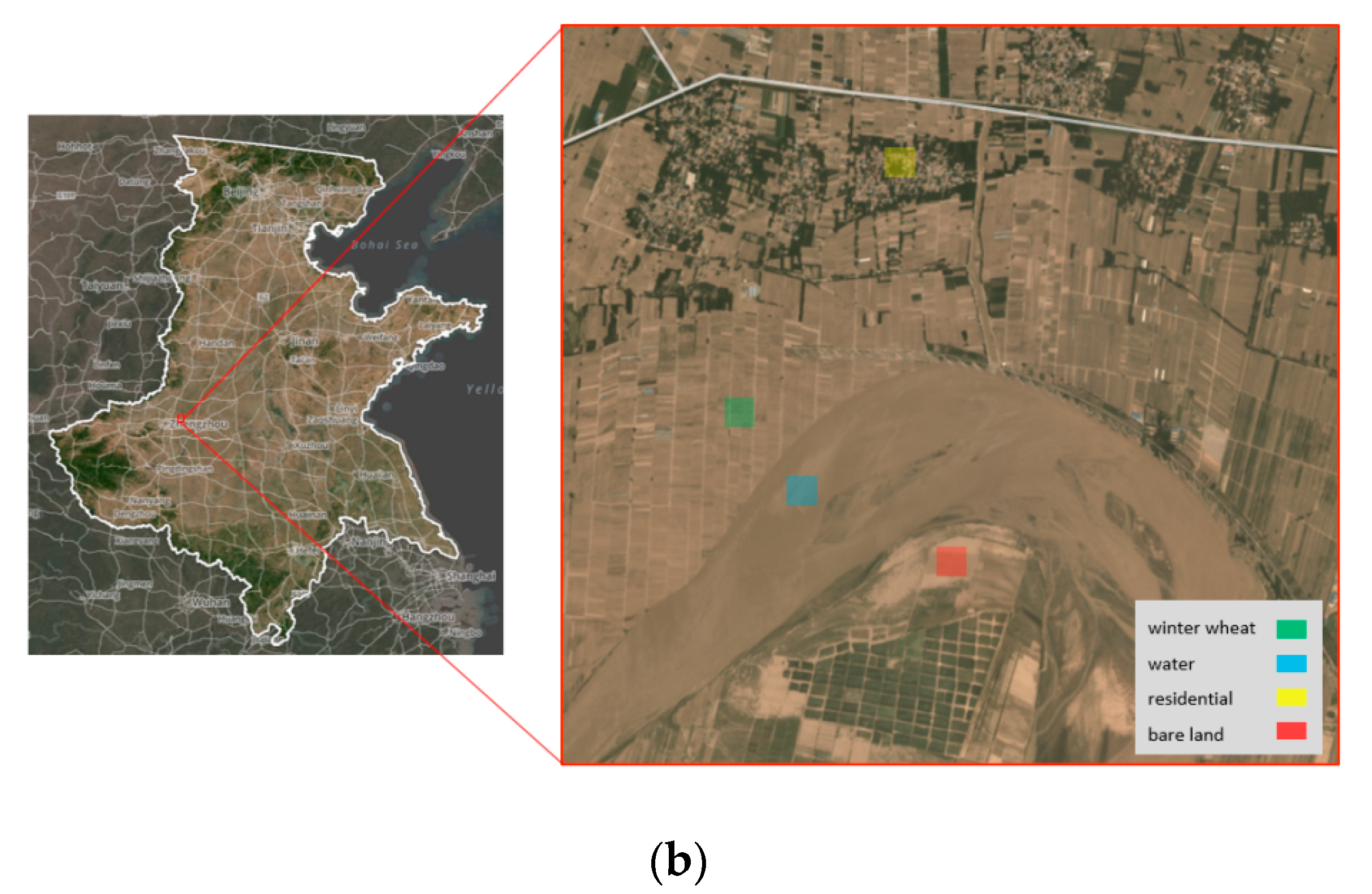
Furthermore, the overall accuracies of our two models were 0.87 and 0.85. However, the precision and recall were approximately 0.70, which is not sufficiently precise for the detailed mapping of winter wheat. This result is mainly due to three phenomena. (1) the cell size of MODIS data is 250 m, and a cell might contain multiple land cover types, thus making the reflectance spectra unstable and unpredictable. (2) Our ground truth map, which was provided by the Chinese Academy of Agricultural Sciences, was assumed to be totally accurate in each cell. Since we did not receive any instructions regarding how to complete the map or information on the data accuracy, we reassessed the data via manually collected field data, as described in Section 2.2.2. The results indicated that the overall accuracy of the ground truth map was 0.95, the precision of winter wheat was 0.89, and the recall was 0.83, which might result in noise in the training sample labels. (3) Although many works have demonstrated the effectiveness of RF and DNNs, they still have limitations in learning the characteristics of such a large and complex area. Using a more complex RF or A-LSTM (a larger number of trees with RF or a deeper network with A-LSTM) could increase the inference ability. However, this usually causes severe overfitting problems, and experiments have shown that the validation score remains almost unchanged when the models reach saturation.
In this paper, we also visualized the feature importance of RF. Generally, the features derived from March or April had high importance scores. In early March, the first joint emerges above the soil line. This joint provides visual evidence that the plants have initiated their reproduction [35]. Then, winter wheat enters a fast-growing period until maturation. Thus, features in this period tend to be significant. For the feature importance of different bands, vegetation indices such as NDVI or EVI represent the reflectance differences between vegetation and soil in the visible and NIR bands. Green vegetation usually exhibits a large spectral difference between the red and NIR bands, thus making the vegetation index more important than a single band. In our study, features were derived from the six bands provided by the MOD13Q1, Collection 6 product. Future work could add additional bands in the models, which might provide better results.
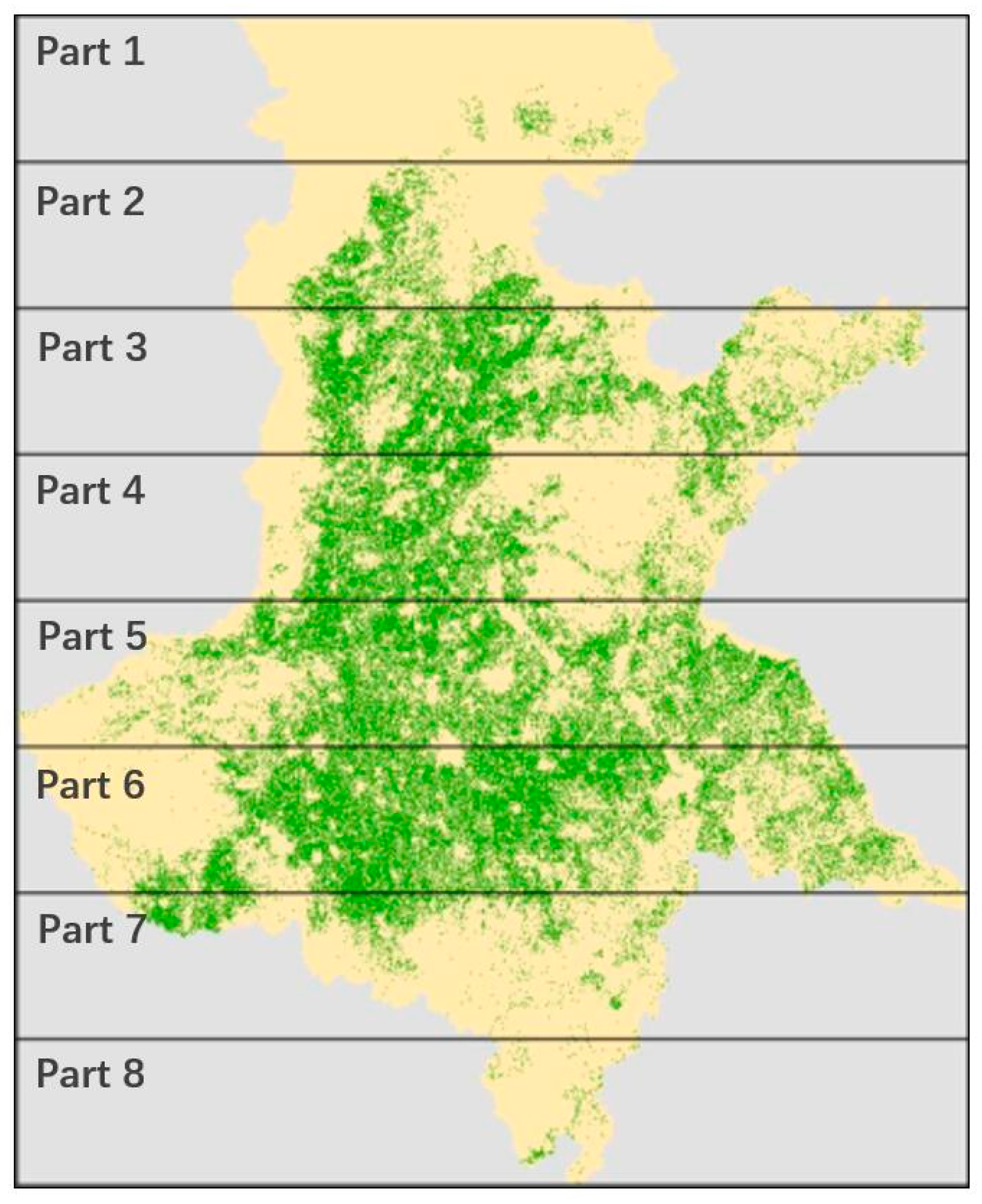
When the trained models are used to make predictions in other areas, close areas usually have reliable results. The main reason behind this result is that the winter wheat growing season varies by area. Specifically, in the Huanghuaihai Region, winter wheat crops at the same latitudes likely have similar growing seasons. In addition, the experiments above support our point of view. Practically, there must be other reasons that result in the poor performance, such as the terrain, elevation, climate, crop species or different land cover compositions of the negative samples. Thus, the MODIS data distribution in the prediction area varies compared to that in the training areas. Our future work will focus on revealing the detailed mechanisms underlying this difference. Fortunately, when we applied our model to historical MODIS data, the performance was stable, as described in Section 4.6. However, exceptions sometimes exist that result in noise in the prediction, such as improved winter wheat species, climate changes, and land cover changes. Regrettably, we did not conduct additional experiments over more past years because of the extensive labor required to collect validation data.

6. Conclusions

In this paper, we developed two models for large-scale winter wheat identification in the Huanghuaihai Region. To the best of our knowledge, this study was the first to use raw digital numbers derived from time-series MODIS images to implement classification pipelines and make predictions over a large-scale land area. According to our experiments, we can draw the following general conclusions. (1) Both the RF and A-LSTM models were efficient for identifying winter wheat areas, with F1 scores of 0.72 and 0.71, respectively. (2) The comparison of the two models indicates that RF achieved a slightly better score than A-LSTM, while A-LSTM is much faster with GPU acceleration. (3) For time-series winter wheat identification, the data acquired in March or April are more important and contribute more than the data acquired at other times. Vegetation indices such as EVI and NDVI are more helpful than single reflectance bands. (4) Predicting in local or nearby areas is more likely to yield reliable results. (5) The models are also capable of efficiently identifying historical winter wheat areas.
Our models were applied to only winter wheat identification due to the limitations of the crop distribution data, but they could potentially solve multiclass problems. Further research regarding multiple crop types or other land cover types over large regions could be more meaningful and useful. Moreover, due to the scarcity and acquisition difficulties of high-spatiotemporal-resolution images, the cell size of each training sample was 250 m, which is too large to avoid the mixed-pixel problem. We believe that using time-series images with finer scales could help improve the accuracy and generalizability of our models. Obviously, it is easy to determine how predictions are determined in RF models, but this information is difficult to determine in the A-LSTM model. Future research will likely devote more attention to the inference mechanisms of DNNs.

Author Contributions

T.H. performed the research, analyzed the data and wrote the manuscript; C.X. provided ideas and reviewed the experiments and the manuscript. S.G. acquired the data. G.L. reviewed the research and provided funding support.

Funding

This research was financially supported by the National Key Research and Development Program of China (No. 2017YFD0300403) and the Laboratory Independent Innovation Project of State Key Laboratory of Resources and Environment Information System.

Acknowledgments

We thank the Chinese Academy of Agricultural Sciences for providing the winter wheat distribution map and growing season data for 2017–2018. We thank the NASA Goddard Space Flight Center for providing the MODIS data.

Conflicts of Interest

The authors declare no conflicts of interest.

References

  1. Becker-Reshef, I.; Justice, C.; Sullivan, M.; Vermote, E.; Tucker, C.; Anyamba, A.; Small, J.; Pak, E.; Masuoka, E.; Schmaltz, J.; et al. Monitoring Global Croplands with Coarse Resolution Earth Observations: The Global Agriculture Monitoring (GLAM) Project. Remote Sens. 2010, 2, 1589–1609. [Google Scholar] [CrossRef] [Green Version]
  2. Eerens, H.; Haesen, D.; Rembold, F.; Urbano, F.; Tote, C.; Bydekerke, L. Image time series processing for agriculture monitoring. Environ. Model. Softw. 2014, 53, 154–162. [Google Scholar] [CrossRef]
  3. Atzberger, C. Advances in Remote Sensing of Agriculture: Context Description, Existing Operational Monitoring Systems and Major Information Needs. Remote Sens. 2013, 5, 949–981. [Google Scholar] [CrossRef] [Green Version]
  4. Beeri, O.; Peled, A. Geographical model for precise agriculture monitoring with real-time remote sensing. ISPRS J. Photogramm. Remote Sens. 2009, 64, 47–54. [Google Scholar] [CrossRef]
  5. Senf, C.; Pflugmacher, D.; Van Der Linden, S.; Hostert, P. Mapping rubber plantations and natural forests in Xishuangbanna (Southwest China) using multi-spectral phenological metrics from MODIS time series. Remote Sens. 2013, 5, 2795–2812. [Google Scholar] [CrossRef]
  6. Pittman, K.; Hansen, M.C.; Becker-Reshef, I.; Potapov, P.V.; Justice, C.O. Estimating Global Cropland Extent with Multi-year MODIS Data. Remote Sens. 2010, 2, 1844–1863. [Google Scholar] [CrossRef] [Green Version]
  7. Tuanmu, M.N.; Viña, A.; Bearer, S.; Xu, W.; Ouyang, Z.; Zhang, H.; Liu, J. Mapping understory vegetation using phenological characteristics derived from remotely sensed data. Remote Sens. Environ. 2010, 114, 1833–1844. [Google Scholar] [CrossRef]
  8. Sakamoto, T.; Yokozawa, M.; Toritani, H.; Shibayama, M.; Ishitsuka, N.; Ohno, H. A crop phenology detection method using time-series MODIS data. Remote Sens. Environ. 2005, 96, 366–374. [Google Scholar] [CrossRef]
  9. Zhang, X.; Friedl, M.A.; Schaaf, C.B.; Strahler, A.H.; Hodges, J.C.; Gao, F.; Reed, B.C.; Huete, A. Monitoring vegetation phenology using MODIS. Remote Sens. Environ. 2003, 84, 471–475. [Google Scholar] [CrossRef]
  10. Funk, C.; Budde, M.E. Phenologically-tuned MODIS NDVI-based production anomaly estimates for Zimbabwe. Remote Sens. Environ. 2009, 113, 115–125. [Google Scholar] [CrossRef]
  11. Jönsson, P.; Eklundh, L. Seasonality extraction by function fitting to time-series of satellite sensor data. Geosci. Remote Sens. IEEE Trans. 2002, 40, 1824–1832. [Google Scholar] [CrossRef]
  12. Jönsson, P.; Eklundh, L. TIMESAT—A program for analyzing time-series of satellite sensor data. Comput. Geosci. 2004, 30, 833–845. [Google Scholar] [CrossRef]
  13. Atzberger, C.; Eilers, P.H.C. A time series for monitoring vegetation activity and phenology at 10-daily timesteps covering large parts of South America. Int. J. Digit. Earth 2011, 4, 365–386. [Google Scholar] [CrossRef]
  14. Chen, J.; Jönsson, P.; Tamura, M.; Gu, Z.; Matsushita, B.; Eklundh, L. A simple method for reconstructing a high-quality NDVI time-series data set based on the Savitzky-Golay filter. Remote Sens. Environ. 2004, 91, 332–344. [Google Scholar] [CrossRef]
  15. Shao, Y.; Lunetta, R.S.; Wheeler, B.; Iiames, J.S.; Campbell, J.B. An evaluation of time-series smoothing algorithms for land-cover classifications using MODIS-NDVI multi-temporal data. Remote Sens. Environ. 2016, 174, 258–265. [Google Scholar] [CrossRef]
  16. Zhong, L.; Hu, L.; Zhou, H. Deep learning based multi-temporal crop classification. Remote Sens. Environ. 2019, 221, 430–443. [Google Scholar] [CrossRef]
  17. Rodriguez-Galiano, V.F.; Ghimire, B.; Rogan, J.; Chica-Olmo, M.; Rigol-Sanchez, J.P. An assessment of the effectiveness of a random forest classifier for land-cover classification. ISPRS J. Photogramm. Remote Sens. 2012, 67, 93–104. [Google Scholar] [CrossRef]
  18. Pelletier, C.; Valero, S.; Inglada, J.; Champion, N.; Dedieu, G. Assessing the robustness of Random Forests to map land cover with high resolution satellite image time series over large areas. Remote Sens. Environ. 2016, 187, 156–168. [Google Scholar] [CrossRef]
  19. Breiman, L. Random forests. Mach. Learn. 2001, 45, 5–32. [Google Scholar] [CrossRef]
  20. Rußwurm, M.; Korner, M. Temporal vegetation modelling using long short-term memory networks for crop identification from medium-resolution multi-spectral satellite images. In Proceedings of the IEEE Conference on Computer Vision and Pattern Recognition Workshops, Honolulu, HI, USA, 21–26 July 2017; pp. 11–19. [Google Scholar]
  21. Rußwurm, M.; Körner, M. Multi-temporal land cover classification with sequential recurrent encoders. ISPRS Int. J. Geo-Inf. 2018, 7, 129. [Google Scholar] [CrossRef]
  22. Krizhevsky, A.; Sutskever, I.; Hinton, G.E. Imagenet classification with deep convolutional neural networks. In Proceedings of the 25th International Conference on Neural Information Processing Systems (NIPS’12), Lake Tahoe, NV, USA, 3–6 December 2012; pp. 1097–1105. [Google Scholar]
  23. Szegedy, C.; Liu, W.; Jia, Y.; Sermanet, P.; Reed, S.; Anguelov, D.; Erhan, D.; Vanhoucke, V.; Rabinovich, A. Going deeper with convolutions. In Proceedings of the 2015 IEEE conference on computer vision and pattern recognition, Boston, MA, USA, 7–12 June 2015; pp. 1–9. [Google Scholar]
  24. He, K.; Zhang, X.; Ren, S.; Sun, J. Deep residual learning for image recognition. In Proceedings of the 2016 IEEE Conference on Computer Vision and Pattern Recognition, Las Vegas, NV, USA, 27–30 June 2016; pp. 770–778. [Google Scholar]
  25. Bahdanau, D.; Cho, K.; Bengio, Y. Neural machine translation by jointly learning to align and translate. arXiv 2014, arXiv:1409.0473. [Google Scholar]
  26. Long, H.; Yi, Q. Land Use Transitions and Land Management: A Mutual Feedback Perspective. Land Use Policy 2018, 74, 111–120. [Google Scholar] [CrossRef]
  27. Zhang, J.; Sun, J.; Duan, A.; Wang, J.; Shen, X.; Liu, X. Effects of different planting patterns on water use and yield performance of winter wheat in the Huang-Huai-Hai plain of China. Agric. Water Manag. 2007, 92, 41–47. [Google Scholar] [CrossRef]
  28. Huete, A.R.; Didan, K.; Miura, T.; Rodriguez, E.P.; Gao, X.; Ferreira, L.G. Overview of the radiometric and biophysical performance of the MODIS vegetation indices. Remote Sens. Environ. 2002, 83, 195–213. [Google Scholar] [CrossRef]
  29. Powers, D.M.W. Evaluation: From Precision, Recall and F-Measure to ROC, Informedness, Markedness & Correlation. J. Mach. Learn. Technol. 2011, 2, 37–63. [Google Scholar]
  30. Scikit-Learn. Available online: https://scikit-learn.org/ (accessed on 1 March 2019).
  31. Tensorflow. Available online: https://www.tensorflow.org/ (accessed on 1 March 2019).
  32. Keras. Available online: https://keras.io/ (accessed on 1 March 2019).
  33. Sebastian, R. An Overview of Gradient Descent Optimization Algorithms. Available online: https://arxiv.org/pdf/1609.04747.pdf (accessed on 3 January 2019).
  34. Yao, Y.; Rosasco, L.; Caponnetto, A. On Early Stopping in Gradient Descent Learning. Constr. Approx. 2007, 26, 289–315. [Google Scholar] [CrossRef]
  35. Li, Z.-C. Hyperspectral Features of Winter Wheat after Frost Stress at Jointing Stage: Hyperspectral Features of Winter Wheat after Frost Stress at Jointing Stage. Acta Agron. Sin. 2008, 34, 831–837. [Google Scholar] [CrossRef]
Figure 1. Location of the study area.
Remotesensing 11 01665 g001
Figure 2. Two images of the same parcel acquired in March 2018 (a) and June 2018 (b) from the Planet Explorer API. In March, winter wheat enters the green-returning stage, while most of the other vegetation is still not germinated. In June, winter wheat enters maturation stage and turns yellow, while other vegetation is green. Therefore, it is easy to distinguish wheat areas and other land cover types using images acquired in the two stages via visual interpretation.
Remotesensing 11 01665 g002aRemotesensing 11 01665 g002b
Figure 3. Geographical partitioning strategy. The whole region was partitioned into eight regions from north to south.
Remotesensing 11 01665 g003
Figure 4. (a) The simple recurrent neural network (RNN) architecture, (b) the attention-based long short-term memory (A-LSTM) architecture, (c) the unrolled chain-type RNN structure.
Remotesensing 11 01665 g004aRemotesensing 11 01665 g004b
Figure 5. Overview of the A-LSTM architecture. The attention mechanism looks at the complete encoded sequence to determine the encoded steps to weigh highly and generates a context vector. The decoder network uses these context vectors to make a prediction.
Remotesensing 11 01665 g005
Figure 6. Fine-tuning of the parameters n and k of the random forest (RF) model, (a) the overall accuracy of the RF trained on pure-mixed pixel set, (b) the overall accuracy of the RF trained on Pure pixel set. When n equals 500 and k equals 40, the performances of RF models converge; thus, we selected this combination for further experiments.
Remotesensing 11 01665 g006
Figure 7. Training logs for the A-LSTM model, (a) model trained on a mixed dataset, (b) model trained on a pure dataset.
Remotesensing 11 01665 g007
Figure 8. (a) The prediction map informed by the RF model, (b) the prediction map informed by the A-LSTM model, (c) ground truth winter wheat distribution map.
Remotesensing 11 01665 g008
Figure 9. (a) Importance scores of 132 variables with the hierarchy indexed by timestep and band, (b) Accumulated importance score per timestep, (c) Accumulated importance score per band.
Remotesensing 11 01665 g009
Figure 10. The mean probability distribution that the target class is aligned with the encoded sequence.
Remotesensing 11 01665 g010
Figure 11. The winter wheat growing season in the Huanghuaihai Region, (a) sowing; (b) overwintering; (c) green-returning; (d) jointing; (e) flowering; (f) maturation. The cell values of the raster map represent the day of the year on which winter wheat enters the growing stage. Contour lines are shown on the map. The first two maps show the growing times in 2017, and the others show the growing times in 2018.
Remotesensing 11 01665 g011
Figure 12. Historical winter wheat distribution map (2016–2017 growing season) informed by (a) RF and (b) A-LSTM, (c) the distribution of manually collected evaluation samples from the Planet Explorer API.
Remotesensing 11 01665 g012
Table 1. Data samples extracted from Moderate Resolution Imaging Spectroradiometer (MODIS) images.
Pure Wheat (1)Pure No-Wheat (0) Mixed   Pixels   Wheat   ( 1 _ ) Mixed   Pixels   No - wheat   ( 0 _ ) Total
62028763385242679611356688913205311
Table 2. The number of samples in each geographically partitioned dataset.
QuantityPart 1Part 2Part 3Part 4Part 5Part 6Part 7Part 8
Pure Pos10693415415901011713213580515839314014710
Pure Neg1313370773568816377829138736828924470685303259470
Mixed8253233985510347897852341568533180218256507468301
Total1396971114757720101761731504244116628850451264391328481
Table 3. Confusion matrix charted by the predicted and actual classification.
Positive (predicted)Negative (predicted)
Positive (actual)True positives (TP)False negatives (FN)
Negative (actual)False positives (FP)True negatives (TN)
Table 4. Precision, recall, overall accuracy and F1 scores for the two models trained on different datasets.
Pure Pixel SetPure-Mixed Pixel Set
RFA-LSTMRFA-LSTM
Precision0.750.740.720.71
Recall0.620.600.710.70
Overall Accuracy0.85 (±0.01)0.82 (±0.01)0.87 (±0.01)0.85 (±0.01)
F1 score0.68 (±0.01)0.66 (±0.01)0.72 (±0.01)0.71 (±0.01)
Table 5. Top 10 variables in order of decreasing importance in the RF model. The first column lists the index in the 132-variable sequence. The second column represents the feature name, which consists of the day of the year and the band name. The third column represents the importance score.
IndexBand/Feature NameImportance
792018081_EVI0.029
812018081_NDVI0.024
852018097_EVI0.023
822018081_NIR0.023
882018097_NIR0.022
1112018161_NDVI0.020
872018097_NDVI0.020
912018113_EVI0.018
732018065_EVI0.015
1052018245_NDVI0.014
Table 6. Generalization performance scores of the RF model.
MetricsTestingGeneralization Evaluation
Fold 4Fold 5Fold 6Fold 7Fold 8
Precision0.7520.7240.6600.7460.7470.602
Recall0.6820.6640.6820.6030.4100.073
Total accuracy0.9060.8450.7590.7860.9130.972
F1 score0.7150.6930.6710.6670.5290.130
Table 7. Confusion matrix of the prediction map informed by RF.
ReferencePrediction
Winter WheatNo-WheatRecall
Winter Wheat85330.720
No-Wheat308520.966
Precision0.7390.963
Table 8. Confusion matrix of the prediction map informed by A-LSTM.
ReferencePrediction
Winter WheatNo-WheatRecall
Winter wheat83350.703
No-wheat298530.967
Precision0.7410.961

