Article

Forward Simulation of Multi-Frequency Microwave Brightness Temperature over Desert Soils in Kuwait and Comparison with Satellite Observations

1
Department of Physics, Kuwait University, P.O. Box 5969, Safat 13060, Kuwait
2
Civil Infrastructure and Environmental Engineering Department, Masdar Institute, Khalifa University of Science and Technology, P.O. Box 54224, Abu Dhabi, UAE
3
Department of Civil and Environmental Engineering, Massachusetts Institute of Technology, Cambridge, MA 02139, USA
4
Disaster Management Program, Kuwait Institute for Scientific Research, P.O Box 24885, Safat 13109, Kuwait
5
Department of Mathematics and Natural sciences, American University of Kuwait, P.O. Box 3323, Safat 13034, Kuwait
*
Author to whom correspondence should be addressed.
Remote Sens. 2019, 11(14), 1647; https://doi.org/10.3390/rs11141647
Submission received: 30 May 2019 / Revised: 7 July 2019 / Accepted: 9 July 2019 / Published: 11 July 2019

Abstract

:
In this study, we address the variations of bare soil surface microwave brightness temperatures and evaluate the performance of a dielectric mixing model over the desert of Kuwait. We use data collected in a field survey and data obtained from NASA Soil Moisture Active Passive (SMAP), European Space Agency Soil Moisture and Ocean Salinity (SMOS), Advanced Microwave Scanning Radiometer 2 (AMSR2), and Special Sensor Microwave/Imager (SSM/I). In situ measurements are collected during two intensive field campaigns over bare, flat, and homogeneous soil terrains in the desert of Kuwait. Despite the prevailing dry desert environment, a large range of soil moisture values was monitored, due to precedent rain events and subsequent dry down. The mean relative difference (MRD) is within the range of ±0.005 m3·m−3 during the two sampling days. This reflects consistency of soil moisture in space and time. As predicted by the model, the higher frequency channels (18 to 19 GHz) demonstrate reduced sensitivity to surface soil moisture even in the absence of vegetation, topography and heterogeneity. In the 6.9 to 10.7 GHz range, only the horizontal polarization is sensitive to surface soil moisture. Instead, at the frequency of 1.4 GHz, both polarizations are sensitive to soil moisture and span a large dynamic range as predicted by the model. The error statistics of the difference between observed satellite brightness temperature (Tb) (excluding SMOS data due to radio frequency interference, RFI) and simulated brightness temperatures (Tbs) show values of Root Mean Square Deviation (RMSD) of 5.05 K at vertical polarization and 4.88 K at horizontal polarization. Such error could be due to the performance of the dielectric mixing model, soil moisture sampling depth and the impact of parametrization of effective temperature and roughness.

Graphical Abstract

1. Introduction

Soil moisture is an important parameter for hydrological, climate, and weather model predictions. Low frequency microwave instruments are used to remotely sense and map soil moisture. At these frequencies, the atmosphere is nearly transparent and the surface reflectivity is sensitive to the Volumetric Soil Moisture (VSM) content. Remotely sensed low frequency microwave measurements are however at low resolution constrained by the antenna size. Hence, heterogeneity of soil moisture is a source of bias and error, especially for the case of space borne retrievals. The spatial and temporal variations of soil moisture from in situ measurements are hence important for the validation of satellite measurements. Several studies in the literature report field experiments to study spatial and temporal variations. A study on a semi-arid region in China found that environmental attributes such as land use and topography play an important role in the spatial distribution of soil moisture content [1]. Various field campaigns in the regions of Oklahoma and Iowa, in the central USA, studied over 36,000 ground-based soil moisture samples [2]. At the field scale, Temimi et al. [3] analyzed the diurnal variability of L-band brightness temperature and its impact on soil moisture retrievals in upstate New York, USA. They showed that soil effective temperature at 12 cm can lead to the most accurate soil moisture retrieval. A temporary network was deployed for upscaling of a sparse network [4]. Another study reported that soil type as characterized by bulk density, clay and sand content, was responsible for 50% of temporal stability, and topographic effects were less important in the stability of soil moisture [5]. Variations of soil moisture in space and time can be related to local features, such as soil properties and microtopography, and non-local features, such as drainage lines [6]. According to Schneider et al. [7] and Ryu et al. [8], temporal stability is important to validate hydrological, remote sensing models, and to upscale soil moisture information to larger scales. The spatial variability of the test site determines the number of samples required to estimate the mean value of soil moisture of the footprint. Several studies investigate the retrieval and the validation of soil moisture at low microwave frequency L-band (1.4 GHz) from the SMAP satellite [9,10,11]. The SMOS satellite mission also uses the low microwave L band frequency to measure soil moisture [12,13]. Attempts to retrieve soil moisture from higher frequencies utilized by such as the SSM/I and AMSR2 satellites were conducted and investigated in several studies [14,15,16,17,18,19].
Remote sensing of soil moisture and field measurement in the desert of Kuwait has a history dating back to the year 2000 [20,21,22]. In a recent study, Wehbe et al. [23] demonstrated a strong relationship between soil moisture, precipitation, and water storage in the Arabian Peninsula using satellite observations. However, the region still lacks field scale studies like the one conducted here.
In this study, we report on the results of extensive field campaigns designed to assess and evaluate the performance of the dielectric mixing model in the desert. The simulated vertical polarized brightness temperature (Tbv) and horizontal polarized brightness temperature (Tbh) are compared with the observed Tb values of SMAP, SMOS, AMSR2, and SSM/I. We assess the sensitivity of Tbv and Tbh to soil moisture, roughness, soil temperature, and satellite incident angles at different satellite frequencies. The field experiment domain is contained in Kuwait and characterized by bare soil (no vegetation) and low topography (flat). Therefore, mainly soil moisture, soil type, soil temperature, and surface roughness contribute to surface microwave emission. The high density of soil moisture sampling within the study domain was useful to analyze the spatial distribution of soil moisture and the effect of surface heterogeneity on satellite retrievals. The objective of this paper is to assess microwave brightness temperatures simulated at specific channels coincident with those onboard SMAP, AMSR2, SMOS, and SSM/I in microwave frequencies ranging from 1.4 GHz to 19 GHz in the Kuwait desert environment. The bare soil and flat conditions across the domain offer a unique opportunity to assess the relationship between microwave frequencies, sensitivity to soil moisture, and surface roughness. Two intensive field campaigns were conducted to collect 322 soil samples from the west side of Kuwait City on both the 20th of February and 19th of March 2016. The samples were collected from every 3 km grid over an area of 36 km × 36 km giving a total number of 144 grids inside the SMAP satellite grid cell in the open desert. The manuscript is organized as follows: Section 2 presents the study area and the methodology that we followed, including a description of the forward brightness temperature model used here. In Section 3, the main results and discussion of our study are presented. Finally, our conclusions are found in Section 4.

2. Methodology

2.1. Study Area

Kuwait is an arid region characterized by its very hot dry summers and mild winters with some rain [24]. There are four seasons in Kuwait: winter, spring, summer and autumn, with sub-seasons of distinct weather, such as frequent dust storms, thunderstorms, or persistent winds. December to mid-February are the wettest and mildest months, and are characterized by south-westerly winds over the Arabian Peninsula. Spring begins in mid-February and generally lasts until May, during which south-easterly winds (Suhaili) bring warm to hot weather, and the Sarrayat (local thunderstorm) is common. Summer is from May until August. During June and July, north-westerly winds may develop, generating extensive dust storms [25]. Autumn starts from the month of September and is characterized by winds switching from the southeast to the northwest. The pattern of winds in the summer is north-westerly due to the summer circulation. The common wind direction in winter is southerly to south-easterly; north-westerly wind in winter is caused by synoptic oscillations. The maximum temperature can be as high as 50 °C or more, while a minimum of −4 °C was recorded at Kuwait International Airport on 20 January 1964. The average rainfall is about 115 mm and varies from year to year (28–260 mm). The evaporation rate ranges from 4.6 mm/day in January to 22.9 mm/day in June [24]. The study area is 36 km × 36 km, coincident with one SMAP soil moisture grid cell as specified in the standard products. The area is located inland on the west side of Kuwait City (Figure 1) at a distance from any water surfaces and has 14 different soil classes [26], as shown in Table 1. The dominant soil classes within the study domain are Cp06, Cp07, Gp03, Gp11, Gp16, and Gp19. The study area is gently sloping (upward) diagonally from northeast to southwest and the elevation varies from 140 m to 220 m.

2.2. Field Campaigns and Satellites’ Data Sets

Two intensive field campaigns were conducted on normal sunny days of 20 February 2016 and 19 March 2016. Rain events were reported from 12 official metrological stations on several days from the first two weeks of February. Several other rain events were also reported between the 20th of February and 19th of March. The total amount of rain recorded was from 1 mm to 15 mm. The air temperatures during the field campaigns and between 7:30 a.m. and 5:30 p.m. were from 15 °C to 29 °C on the 20th of February and 14 C °to 23 °C on the 20th of March.
The design of the field campaigns included intensive spatial sampling of soil moisture, soil texture, bulk density, and soil roughness statistics. These geophysical parameters together with land surface temperatures (LST) are used in a forward microwave emission model (described later) to simulate Tbs at various frequencies and different incident angles of SMAP, SMOS, AMSR2, and SSM/I. The LST is obtained from Meteosat Second Generation/ Spinning-Enhanced Visible and Infrared Imager (MSG/SEVIRI) data set, which is recorded every 15 min. The LST values used in this study are only those that were taken at the same time of the satellite orbit pass. This is to avoid errors in the simulated Tbs due to diurnal variations. The simulated Tbs are then compared with the observed satellites’ Tbs at both vertical and horizontal polarization. The observed brightness temperature was acquired by (SMAP) radiometer during 6:00 a.m. descending and 6:00 p.m.. ascending half-orbit passes. The SMAP Level-1B radiometer brightness temperature product was downloaded from the National Snow and Ice Data Center (NSIDC) website and extracted at an incidence angle of 40° with a spatial resolution of 36 km. SMOS Tb data is from the Level 1C Brightness Temperature product. Each grid point contains a brightness temperature sample interpolated from Microwave Imaging Radiometer using Aperture Synthesis (MIRAS) measurements at an incidence angle of 42.5°. The data are geo-located in an equal-area grid system with a 15 km resolution are downloaded through SMOS online dissemination service websiteAMSR2 Tb L1R data product are from the website of Japan Aerospace Exploration Agency (JAXA) Globe Portal System and extracted at an incidence angle of 55° with a spatial resolution of 25 km. The SSM/I data product is from version 2 at Level-3, have been downloaded through (NSIDC) website and extracted at an incidence angle of 53.1° with a spatial resolution of 25 km. The satellite frequencies, resolution, incident angle, and orbit pass time are shown in Table 2.
The campaigns started from 7:30 a.m. and ended at 5:30 p.m. Both ascending and descending passes were selected depending on the availability of the satellite data around the two field dates in February and March as shown in Table 2. For the 20th of February, only descending data at 6:00 a.m. is available for SMAP, while both ascending (6:00 p.m.) and descending (6:00 a.m.) data are available for the 18th of March, which is the closest to the field campaign day of the 19th of March. SMOS data are not available on the 20th of February, so the closest pass to the field campaign is the descending data at 6:00 p.m. on the 19th of February. The SMOS ascending data at 6:00 a.m. are available for the field campaign day of 19th of March. AMSR2 ascending data at 1:30 p.m. are available for both field days of 20th of February and 19th of March. SSM/I satellite data are not available for the same days of the field campaigns and the closest data available are the ascending pass at 6:30 p.m. on the 19th of February and 18th of March. The effect of the date and time differences of the satellite passes on the results of this study is discussed later in Section 3 and Section 4.

2.2.1. Soil Moisture Sampling

The test site of 36 km × 36 km (Figure 1) was divided into three sections to be sampled for every 3 km2 grid by three teams in order to cover the whole area during the daytime. The sampling was conducted with soil sample canisters that are 5 cm deep. A discussion on the effect of sampling depth for different microwave frequencies is found later in Section 3.3. A total of 156 samples (144 samples plus 12 more samples) were collected for the top 5 cm on 20th February 2016 and 166 samples (144 samples plus 22 more samples) were collected on 19th March 2016, adding to a total of 322 samples. The soil samples were weighed then dried in an oven with a temperature of 105 °C for 48 h. The thermogravimetric method is labor intensive but also the most reliable way to estimate volumetric water content. Other soil moisture monitoring devices, such as those based on wave guides heat dissipation, require a priori onsite calibration curves which are ultimately performed against the thermogravimetric method. After drying, both the bulk density and gravimetric soil moisture are calculated to estimate the volumetric soil moisture. The elevation at the middle of each 3 km sub-grid was measured and stored using a GPS unit. The survey starts at the upper left corner of the grid, and ends at the lower left corner. The starting point is considered as sample point 1 and the end point as sample point 144. The elevation varies from 148 m to 242 m. The southwestern side of the test site shows a high elevation value, while the northeastern side demonstrates low elevation.

2.2.2. Soil Texture and Roughness

Soil texture and roughness were measured for the major six soil types out of 14 different soil types (i.e., the largest in area size, Table 1). Soil texture was determined using the sieving method and it was found that sand and mud fractions vary for different soil types. The range of sand fractions is 80% to 94%, as expected for deserts, whereas the clay varies between 2% and almost 6%, as shown in Table 2.
The soil roughness was measured with the pin profilometer, which consists of 144 pins, each of 60 cm height. It is fixed on a wooden board structure with a graph attached. An image of the profilometer in each location was captured using a high-resolution camera. Three high-resolution images of the pin profilometer were taken for each site. Then, these images were analyzed to obtain the roughness root mean squared (RMS) height and exponential correlation length scale of each soil type.

2.2.3. Land Surface Temperature

Land surface temperatures (LST) used in this study to simulate the brightness temperatures, as mentioned in Section 2.2, are from the Meteosat Second Generation/Spinning-Enhanced Visible and Infrared Imager (MSG/SEVIRI) data. MSG/SEVIRI is an operational product of the Land Surface Analysis Satellite Applications Facility (LSA SAF). The Spinning Enhanced Visible and Infrared Imager (SEVIRI) radiometer embarked on the MSG platform encompasses unique spectral characteristics and accuracy, with a 3 km resolution (sampling distance) at nadir (1 km for the high-resolution visible channel), and 12 spectral channels. The spin-stabilized MSG provides diurnal coverage with an imaging-repeat cycle of 15 min.
The LST/MSG data were downloaded from the Satellite Application Facility on Land Surface Analysis (LSA SAF) website which is part of the distributed European Organization for the Exploitation of Meteorological Satellites (EUMETSAT). As the LST/MSG data were recorded every 15 min, only the LST values at the same time of each satellite pass were used in the model simulation. For the SMAP satellite, LST values of 1 km resolution were averaged over 36 km × 36 km pixels, while for AMSR2 and SSM/I, the LST values were averaged over the grid size of 25 km × 25 km. For SMOS, the LST values were averaged over 15 km × 15 km. Hence, SMAP has one LST value over the test site, but AMSR2 and SSM/I cover four grids inside and around the test grid, while SMOS covers 10 grids. A map of the grids of each satellite inside the test site area is shown in Section 2.3. The averaged LST values, which are used here to calculate Tbs from the forward model, are shown in Table 2.

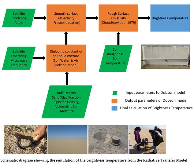
2.3. Forward Brightness Temperature Model

We use the Dobson model [27] to simulate the surface brightness temperature based on the soil dielectric constant, physical temperature, and surface roughness. A discussion on results and the evaluation of using this model is found in Section 3.2. The Kuwait desert test site represents an area with almost no vegetation as described before. Hence, it is a suitable site to study the effects of surface conditions alone (without the confounding effects of vegetation and their inaccurate parameterization).
For a smooth and homogenous surface, Fresnel equations are applied to model reflectivity from the half-space at and below the surface. The vertical and horizontal polarization are derived from electromagnetic theory [28]:
r v = | ϵ r c o s θ ϵ r s i n 2 θ ϵ r c o s θ + ϵ r s i n 2 θ | 2 ,
r h = | c o s θ ϵ r s i n 2 θ c o s θ + ϵ r s i n 2 θ | 2 ,
where r v and r h   represent the reflectivity of horizontal and vertical polarization states, respectively, θ is the incident angle and ϵ r is the complex dielectric constant of the medium. The dielectric constant depends on many different soil parameters, such as soil moisture, soil structure, and bulk density. In this study, ϵ r   is determined from the semi-empirical mixing model of Dobson [27], described by four components: dry soil, bound water, free water, and air:
  ϵ m = [ 1 + ρ b ρ s ( ϵ s α 1 ) + m v β ϵ f w α m v ] 1 α ,
ϵ m = [ m v β ϵ f w α ] 1 α ,
where ϵ m and ϵ m are, respectively, the dielectric constant and loss factor of moist soil,   ϵ s is the dielectric constant of the soil solids, m v is the volumetric moisture content, ρ b is the bulk density in g·cm−3 , and   ρ s is the specific density of the soil solids, which in this study is taken as 2.66 g·cm−3. The quantities ϵ f w   and ϵ f w are the dielectric constant and loss factor of free water. The values of α = 0.65 , β   and β , are empirically determined constants which depend on sand fraction ( S ) and clay fraction ( C ) and are given by the following equations:
β = 1.275 0.519 S 0.152 C ,
β = 1.338 0.603 S 0.166 C .
The dielectric constant of soil solids is calculated as:
ϵ s = ( 1.01 + 0.44 ρ s ) 2 0.062 ,
where ϵ f w and ϵ f w are derived at a given frequency assuming a Debye-type relaxation, as modified by Lane and Saxton [29] to account for ionic conductivity losses and are calculated as follows:
ϵ f w = ϵ w 0 ϵ w 1 + ( 2 π   f τ w ) 2
and
ϵ f w = 2 π   f τ w ( ϵ w 0 ϵ w ) 1 + ( 2 π   f τ w ) 2 +   σ m v 2 π ϵ 0 f ,
where ϵ w (equal to 4.9) is the high–frequency limit of ϵ w , ϵ w 0 is the static dielectric constant of water, f   is the frequency in hertz, τ w is the relaxation time of water, σ m v is the effective conductivity of water in S·m−1 and ϵ 0 is the permittivity of free space equal to 8.854 × 10⁻¹² F·m−1. The known temperature and the static dielectric constant of water, the relaxation time and iconic conductivity are calculated from empirical expressions by Stogryn [30].
The relaxation time of water is obtained from:
τ w = 1 2 π ( 1.1109   x   10 10     3.824   x 10 12 ( T s o i l 273.15 )   +   6.938   x 10 14 ( T s o i l 273.15 ) 2 5.096   x 10 16   ( T s o i l 273.15 ) 3 .
For bare soils, the brightness temperature is the product of the surface emissivity and physical temperature. For a perfectly smooth bare soil with uniform temperature   T s , the soil brightness temperature T b s p becomes:
T b s p = e 0 p   T s ,
where e 0 p = 1 r 0 p ( θ ) .
The rough surface reflectivity, r s p , is related to the smooth soil r 0 p [31] by simple empirical expression:
r s v = [ ( 1 Q ) r 0 v + Q r 0 h ] e x p ( h ) c o s N R P ( θ ) ,
r s h = [ ( 1 Q ) r 0 h + Q r 0 v ] e x p ( h )   c o s N R P ( θ ) ,
where h is a height parameter and Q is a polarization mixing parameter. NRP is introduced to better account for multi-angular and dual-polarization measurements. In an initial study [31], NRP (P = V, H) was set equal to 2, where, in our study, it is approximated to zero. In addition, Q can be approximated to zero at the L-band [31]. Therefore, for 1.4 GHz:
r p =   r 0 p   e x p ( h ) .
p refers to the orthogonal polarization (v or h). A discussion on the effect of approximating both Q and N parameters to zero on the simulated Tb is found in Section 3.3.
The brightness temperatures for SMAP and SMOS are calculated at the L-band (~1.4 GHz), across which the atmospheric effect has negligible impact. However, for AMSR2 and SSM/I, the brightness temperatures are simulated for higher frequencies. It is worth mentioning the effect of the atmosphere is more significant at higher frequencies than for the L, C, and X bands. In the case of SSM/I and AMR2, we do not consider in this study the 37, 85, and 89 GHz frequencies because of the potential significant atmospheric effect, especially in the presence of high water in the atmosphere in the study region as a result of the high evaporation rate. We assume that the atmospheric effect is not significant at lower frequencies.
Figure 2 shows the flow-chart of the process we followed to simulate brightness temperatures from the model described above. The data collected during the intensive field campaigns, namely the mean VSM, soil bulk density, sand/clay fraction, soil roughness and LST inside each satellite grid cell, were used as input parameters for the model (Table 2). The satellite input parameters were incidence angle and the microwave frequency. A total of 63 different grids from all satellites used in this study with their averaged input values to simulate Tbs from February and March field data are shown in Table 2.
The SMAP grid, which is shown as a yellow square in Figure 3, has only one descending pass on the 20th of February and both descending and ascending passes on the 18th of March as shown in Table 2. Therefore, simulations were conducted for three different times over the whole 36 × 36 km test site. However, SMOS (1.4 GHz) was posted at 15 km and therefore 10 grids in February, and another time for the same 10 grids in March, were simulated inside the test site in Figure 3. Some of these pixels have small partial areas inside the test site and were included in the simulation. The AMSR2 simulated brightness temperatures were for four different frequencies (6.9 GHz, 7.3 GHz, 10.7 GHz, and 18.7 GHz). The posting of AMSR2 is 25 km and therefore four simulations for each frequency were carried out within the 36 km × 36 km test site. This results in a total of 32 different input values to simulate Tbs for February and March field data (Table 2). SSM/I simulated brightness temperatures were only for the 19 GHz frequency with a posting of 25 km. This results in eight different values to simulate Tbs for both February and March field data (Table 2). These microwave products, regardless of data posting, have −3 dB half-power resolution in the 40 to 60 km range [9]. The data at the posting are based on overlapping samples around the center of the grid. The values reflect the area at the center of the posted grids and hence are used in the forward model with the in situ conditions of that grid. Figure 3 shows that AMSR2, SMOS and SSM/I are partially sampled. The effect of this mismatch on the simulated brightness temperatures is discussed in the next section.

3. Results and Discussion

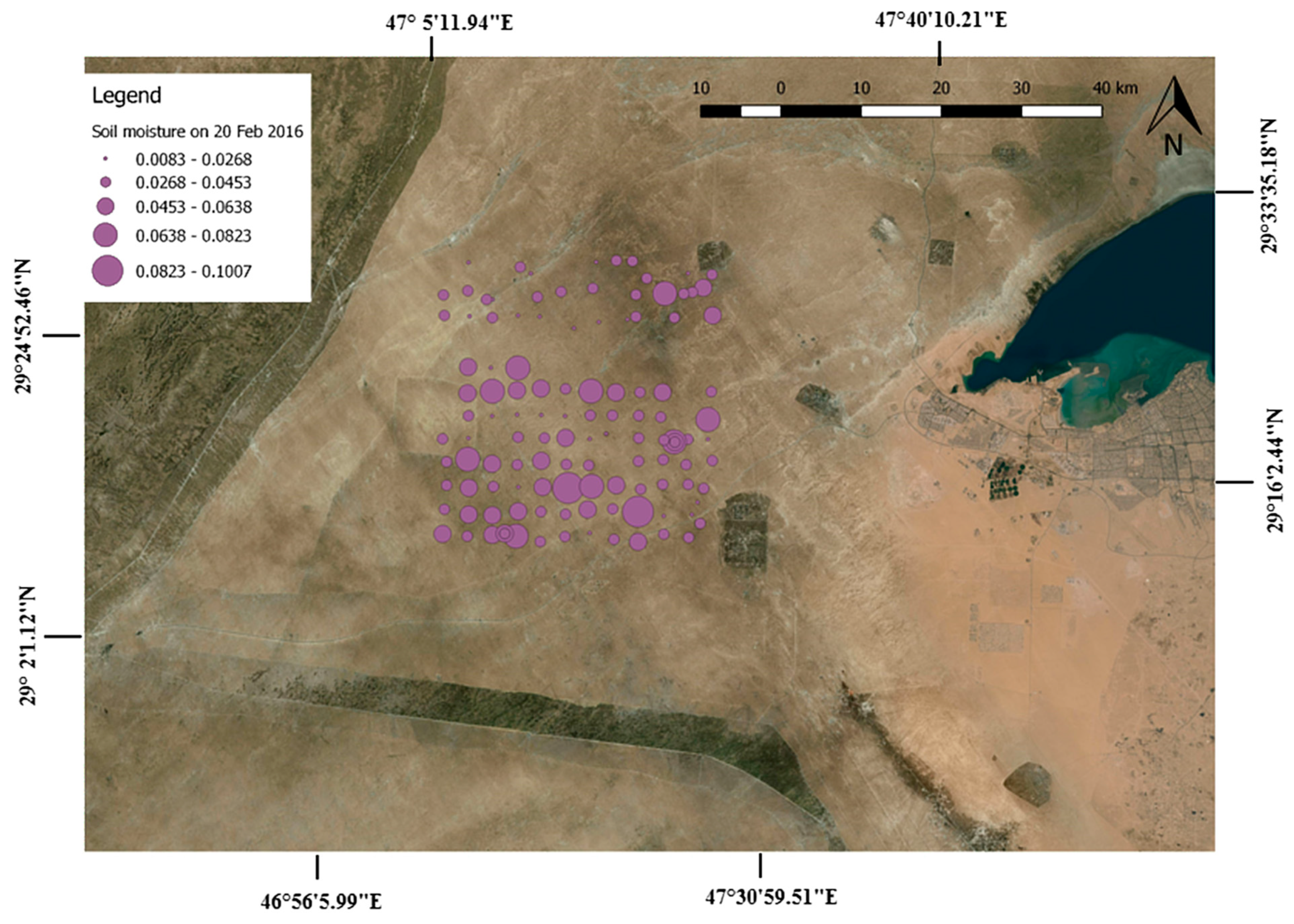
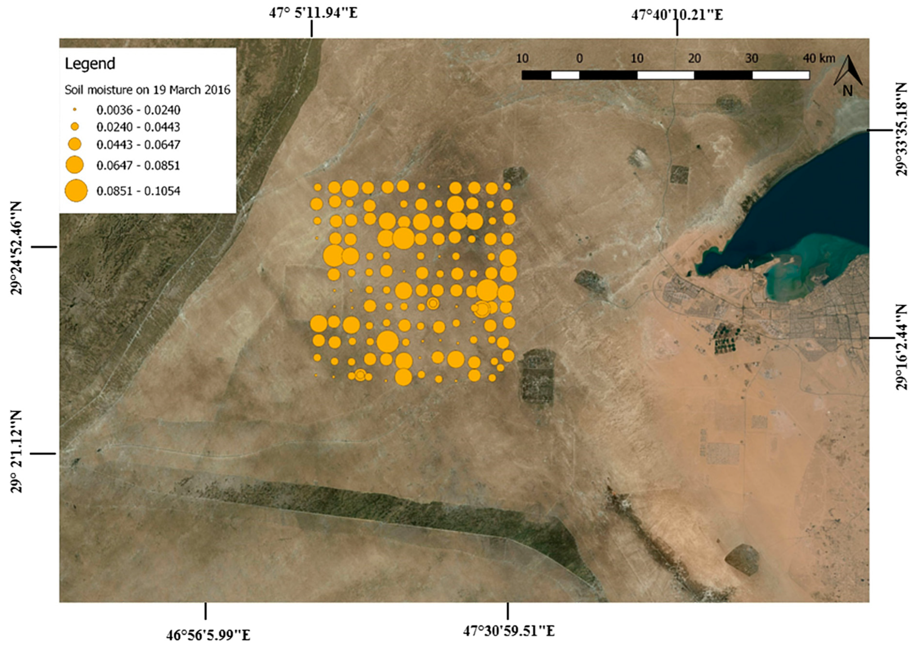
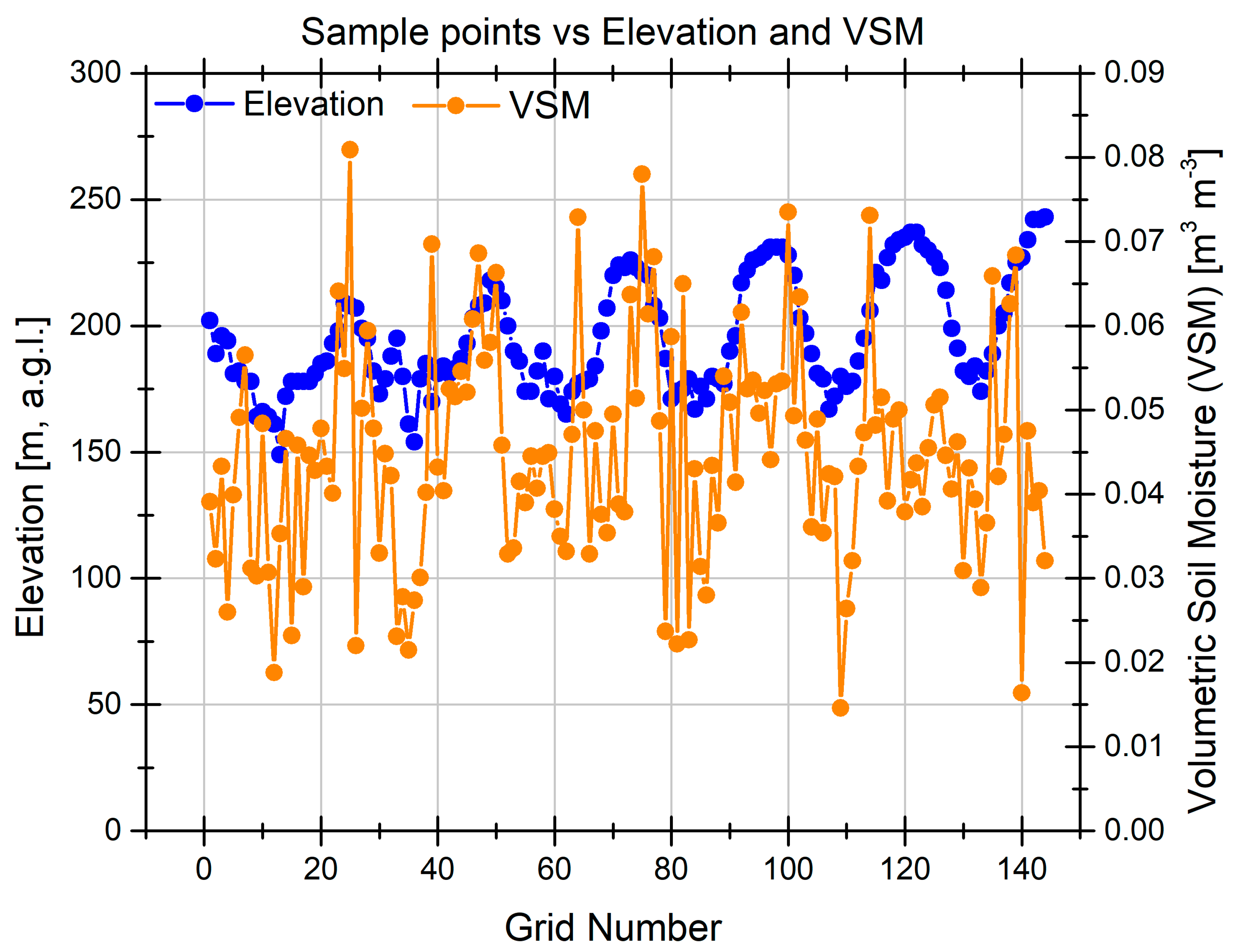
3.1. Analysis of In Situ Observations

The results from the collected 322 samples collected over the whole 36 km × 36 km site and from 7:30 a.m. to 5:30 p.m. are displayed in Figure 4 and Figure 5 for 20 February 2016 and 19 March 2016, respectively. The spatial distribution of the measured VSM showed a significant spatial variability. Higher soil moisture values are noticeable across the field study with a higher concentration in the southern part on 20 February 2016 and in the northern part of the study area on 19 March. The latter is close to a farm on the northeast corner where irrigation could have influenced the soil water content.
The volumetric soil moisture varies from a minimum of 0.008 m3·m−3 to a maximum of 0.101 m3·m−3 with an average value of 0.037 m3·m−3 and standard deviation of 0.016 on the 20th of February (Figure 4). On the 19th of March, the soil moisture varies from a minimum 0.004 m3·m−3 to a maximum of 0.105 m3·m−3 with an average value of 0.045 m3·m−3 and standard deviation of 0.019 m3·m−3 (Figure 5). Hence, dry soil conditions were prevailing on both sampling days despite the fact that the surveys were conducted a few days after the occurrence of rainfall events. This is typical for desert soils and could be attributed to the high evaporation rate in the region. In addition, the high soil porosity should favor a rapid drainage of soil moisture and infiltration towards the water table. The infiltration of soil moisture and its spatial distribution should depend on the soil type and texture as well as the topography of the site. The heterogeneity of the soil in the study area (Figure 1) should control the spatial distribution of soil moisture. A sensitivity analysis was conducted to show the effect of variations of VSM between a minimum of 0.004 m3·m−3 and a maximum of 0.1 m3·m−3 correspond to 28 K in the vertical polarization and 44 K in the horizontal polarization at a low frequency of 1.4 GHz. However, for 19 GHz, the difference decreases to 7 K for vertical polarization and 28 K for horizontal polarization.
To assess the consistency of the measurements across the study site, the mean relative difference (MRD) , δ i ,   of VSM is calculated using:
δ i =   j = 1 n S i j S j S j ,
where Sij is the jth sample at the ith site among the n sites within the study region. Sj is the computed average among all sites for a given date. Figure 6 shows the mean relative difference (MRD) of VSM versus grid number for all the 322 samples collected in the two days, and at different times during the day from morning until evening, to study the spatial and temporal variations of soil moisture. The obtained MRD values were around ±0.005 m3·m−3. Such values of MRD correspond to ~1.2 K in microwave brightness temperature. Although the range of MRD values reflected a certain consistency of soil moisture observations in space and time, the variability of the MRD values within that range during the two sampling days indicated the presence of differences of soil moisture values within the study site, which could be attributed to the soil heterogeneity.
The investigation of soil moisture over the test site is expanded further by determining the effect of elevation on the soil moisture value. The VSM value was averaged for each of the two samples taken from the same sub-grid in February and March. Figure 7 shows higher soil moisture values are obtained at higher elevations, which is counter-intuitive as soil wetness is expected to be higher in depressions and at low points. This could be attributed to the specific drainage pattern in a desert environment where wind, especially the common northwesterly Shamal wind in the region, favors an accumulation of fine soil particles in the low points, while the desert’s physical crust dominates the high points [32]. The accumulation of soil particles in the low points fosters water infiltration to deeper layers, which are not sensed by microwave measurement nor reflected in the gravimetric sampling that is done in this experiment at the 5 cm depth. On the other hand, higher points correspond to more consolidated soil because of the effect of the wind. Such soil should have a lower hydraulic permeability than that at lower points, which should lead to slower drainage, vertical and lateral, and therefore higher wetness at the top soil layer. Such a spatial pattern and relationship between topography and soil moisture spatial distribution are specific to arid region processes like those studied here.

3.2. Verification of the Forward Model in the Desert Environment

The bare forward surface emission model demonstrated in Section 2.3 is used to simulate Tbv and Tbh from the input parameters listed in Table 2 for SMAP (1.41 GHz), SMOS (1.4 GHz), AMSR2 (6.9 GHz, 7.3 GHz, 10.7 GHz and 18.7 GHz), and SSM/I (19 GHz). Figure 8a,b show the comparison between the simulated Tbs from the model and the observed Tbs from these satellites at both vertical and horizontal polarizations, respectively. The lower frequency shows greater dynamic range and match with simulated brightness temperatures from in situ field measurements as inputs. The SMAP 1.4 GHz measurements show good matches with the forward model results. The SMOS 1.4 GHz observed Tbv values demonstrate a considerably high warm bias (Figure 8a), which could be attributed to radio frequency interference (RFI) [33]. However, the SMOS measured Tbh values demonstrate both cold and warm biases (Figure 8b). However, such bias in Tbh is much less than the bias in Tbv. On the other hand, the SMAP radiometer, which has RFI detection and mitigation capabilities, seems to be less affected.
At mid-range microwave AMSR2 frequencies (C and X bands), the vertical channel measurements (Figure 8a) are uncorrelated with the forward model simulations but the horizontal polarization satellite measurements are better correlated. Figure 8a (vertical polarization) shows grouping of AMSR2 (orbital pass at 1:30 p.m.) compared to Figure 8b (horizontal polarization). This is because the Tbv compared to Tbh is more sensitive to LST when it reaches about 38 °C at the 1:30 p.m. orbital pass for AMSR2. Such sensitivity is discussed later in this section. At the highest AMSR2 and SSM/I frequencies (18.7 and 19 GHz, respectively), even for bare soils, the satellite measurements at both polarizations cannot track changes in surface soil moisture, which could be attributed to not accounting for atmospheric effects in the simulation of the model. The atmospheric effect is more significant at higher microwave frequencies [34]. One can state that atmospheric water vapor is particularly high in the region given the proximity to the Gulf, a shallow water body, which is exposed to high temperature and therefore generates strong evaporation. It is worth mentioning here that Figure 8a,b show variations of brightness temperatures with different parameters including soil moisture, LST, satellite incident angle, soil roughness, soil texture and bulk density.
A sensitivity analysis is carried out by simulating the brightness temperature at both v and h polarization for different LSTs, satellite incident angles and frequencies. The results are shown in Figure 9a–c. The simulated brightness temperatures at vertical polarization show more sensitivity to satellite incident angle, frequency, and LST compared to horizontal polarization. The forward model used in this study predicts such sensitivity to LST for the vertical polarization compared to the horizontal polarization as shown in Figure 9a. This might explain the grouping in Figure 8a of AMSR2 (orbital pass at 1:30 p.m.) compared to Figure 8b (horizontal polarization). In addition, Figure 9b shows a higher sensitivity of vertical polarization compared to horizontal polarization when incident angle increases from about 40° for SMAP and SMOS to about 50° or 55° for AMSR2 and SSM/I. Note that the sensitivity of brightness temperatures with frequencies decreases as satellite incident angle increases. Figure 9c shows the variation of Tbs for different frequencies. However, the incident angles used here are from 40° to 55° and, therefore, the sensitivity of Tbs with frequencies at such high angles is weak as predicted by the model. This explains why all AMSR2 frequencies in Figure 9c have almost the same Tbs. The variations of Tbs in Figure 9c is mainly due to LST differences. This is clearly seen from AMSR2 (18.7) and SSM/I (19), which have almost the same frequency; however, the Tb of AMSR2, which has a passing time at 1:30 p.m., is more than the Tb of SSM/I, which has a passing time at 6:30 p.m.
The sensitivity of Tbv to variations in LST is shown clearly from the high values of Mean Difference MD and Root Mean Square Deviation RMSD in Table 3a,b. This is due to the uncertainty in the effective temperature, which affects the vertical polarization more than the horizontal. Both Table 3a,b show statistics of the differences between observed and simulated Tbs. Table 3a includes SMOS results and shows higher values of MD and RMSD compared to Table 3b, which excludes SMOS data. Such high values of MD and RMSD in Table 3a might be due to RFI in SMOS data. In addition, both tables show higher values of MD and RMSD for the vertical polarization, which is more sensitive to LST variations when compared to the horizontal polarization.
Although Table 3b shows lower MD and RMSD and higher correlation coefficients (R) values, MD and RMSD values are considered relatively high, which could be partially attributed to the performance of the Dobson model over our sandy test site. A study by Montpetit et al. [35], which was conducted over sites of silty clay loam bare soil with low sand fraction, found that the Mironov model performs slightly better than the Dobson model at lower frequencies below 11 GHz. However, at higher frequencies than 23 GHz, both Mironov and Dobson models need improvement. A previous study [35] is restricted to a unique area of silty clay loam which may or may not apply to our sandy soil test site. Another study by Srivastava et al. [36] focused on the comparison between four different dielectrics models: Dobson [27], Mironov [37], Wang and Schmugge [38] and Hallikainen [39]. They found that the Mironov model is slightly better at retrieving soil moisture. The test site of Srivastava et al. [36] is sandy loam covered with corn, which is significantly different from our test site characteristics, and they used a single channel algorithm at horizontal polarization to retrieve soil moisture at the L band (1.4 GHz). A case study over a Tibetan sandy soil site [40] assessed the performance of the SMAP soil emission model and the soil moisture retrieval algorithm. They found that the SMAP emission model largely underestimates the SMAP measured Tbh by 15 K and Tbv is underestimated during dry-down episodes. Another study [40] found that the dielectric mixing model proposed by Mironov [41] performs better than the one developed by Dobson [27]. More details on the performance of the Dobson model is discussed in Section 3.3.
Another reason that could explain the discrepancies between the simulated and observed brightness temperatures is the mismatch between LST and effective temperature [31,42,43]. The use of LST estimates in the study to force the radiative transfer model assumes that the penetration depth is zero and that deeper soil layers are not emitting in the microwave. Such an assumption does not necessarily stand in a desert environment where the prevailing soil is sandy and hence has high porosity, which may favor a deeper signal penetration. On the other hand, desert soils tend to have a high quartz content, which increases the soil thermal conductivity and therefore the heat propagation to deeper layers. More discussion on the effective temperature is found in Section 3.3. In addition, the errors seen in Table 3 may be due to the mismatch between 5 cm field sampling and the actual microwave sampling depth, which should contribute to the layer in which dielectric properties dominate the emissivity of surface soil. This is discussed more in Section 3.3.
Errors in roughness could be another source of the discrepancies between simulated and observed Tbs, which contribute to Table 3 statistics. Several studies have suggested that the effective roughness parameters are more suitable than surface roughness and that the angular effect of the incident angle of the satellite should be also considered [11,44,45,46,47]. Such an angular effect of the incident angle is introduced by the NRP parameter in Equations (12) and (13) to better account for multi-angular and dual-polarization measurements [11,45]. In the initial study of [28], NRP (P = V, H) was set equal to 2. In another study [48], the authors found the NRP dependence is too strong and proposed setting NRP = 0. Since then, the values of NRP equal to −1, 0 or 1 have been widely used in the literature [42,49]. Another study [50] showed that the values of NRP for both H and V polarizations should not necessarily be the same. In the desert test site of Kuwait, Q and NPR were set to zero in Equations (12) and (13) as an approximation, which might work well for the L band of SMAP and SMOS, but might also cause some uncertainty in simulated Tb, as seen from Figure 8a,b, especially for high frequencies of AMSR2 and SMOS. Most of the published studies specify or assume that the value of Q increases with frequency, from a value close to 0.0 at the L-band, and ~0.1 at the C-band, to 0.2–0.3 at the X-band [11].

3.3. Discussion

In this study, we see a large difference between the simulated Tb and satellite Tb when SMOS data are included with RMSD value ranges between 10 K (for horizontal polarization) and about 21 K (for vertical polarization). Such high values of RMSD are mainly due to the impact of RFI. However, when SMOS data are excluded, then RMSD drops to values between 4 K and 5 K as shown in Table 3b, which might be attributed to different factors, such as the performance of the Dobson dielectric mixing model. The complex dielectric constant of bound water plays an important role in the determination of the dielectric constant of moist soil [37,38,51]. In the Dobson model [27], an approximation is made to the complex dielectric constant of bound water and its volume fraction, expressed as m v β ϵ f w α in Equation (3), as described by Dobson et al. [27]. Such approximation of the complex constants of bound water might cause some error in the calculated Tb [52], especially for our test site, which has a very low range of VSM (less than 0.1 cm3·cm−3). Other sources of uncertainty in Dobson’s model might be related to organic matter, bulk density, and salinity [53,54].
Another factor that could explain the RMSD values is using soil moisture samples collected earlier or later compared to the satellite overpassing time. For instance, SMAP data were not available on the sampling day of the 19th of March and the closest pass was on the 18th of March. Similarly, we choose the closest orbit pass for both SMOS and SSM/I. Finally, the mismatch between different satellite grids inside the test site is another contribution to such error. This is clear from Figure 3, which shows AMSR2, SMOS and SSM/I are partially sampled. Although the test site is homogeneous and shows stability in space and time, it shows a variability of VSM with mean relative difference (MRD) equal to ±0.005 m3·m−3 (Section 3.1), which corresponds to ~1.2 K error in microwave brightness temperature. It is worth mentioning that such sensitivity of Tb with soil moisture variations increases as frequency decreases, and is more evident at horizontal polarization as predicted by the model.
The soil moisture sampling depth is defined as the depth of the soil layer in which dielectric properties dominate the emissivity of surface soil [55,56,57,58]. Many experimental and theoretical analyses [56,57] lead to the conclusion that the microwave sampling depth in soils is about one-tenth of the wavelength of observation. Research conducted by Escorihuela et al. [50] found that, for dry soils, the best correlation was obtained between brightness temperature at the L-band and soil moisture over the first 2 cm, whereas for wet soils, the best correlation was between brightness temperature and soil moisture measured over the 0 to 1 cm surface layer. In this study, the soil sampling was conducted for the first 5 cm and the averaged retrieved VSM over the different footprints for each satellite was then used to simulate Tbs for all frequencies from 1.4 GHz up to 19 GHz. Although it is known that the 5 cm layer is representative of the effective depth affecting emissions at 1.4 GHz and that higher frequencies are actually sensing shallower layers, e.g., in the order of a few millimeters in the case of 37 GHz, this does not necessarily match the sampling depth of microwave emissions at the L-band or even the other higher frequencies used in our study. Such mismatch can bring uncertainty in the simulated Tb. Nevertheless, other studies indicated that the actual effective depth would depend always on soil moisture in addition to other factors like the satellite angle and soil textures. A study conducted by Owe et al. [59] compared soil moisture penetration depth for different soil textures and bulk densities, and found that the microwave radiometers can sometimes see more than the defined theoretical penetration depth depending on soil moisture conditions and soil texture. Furthermore, the sandy soils are mostly dry in this region. Hence, the microwave sensing depths may be relatively large at the studied frequencies which could contribute to uncertainties in the simulated Tb.
The vertical profile information on both soil moisture and soil temperature is important to formulate the effective temperature. Temperature profiles have a significant effect on microwave emission, especially at lower microwave frequencies [55]. A study conducted by Temimi et al. [3] demonstrated that the effective temperature at 1.4 GHz corresponds to 12 cm in loamy sand with a high rock fraction, which may have favored a deeper penetration of the signal. Previous studies showed that the use of the theoretical effective temperature improves the estimations of brightness temperature by not more than 0.1 K [57]. The mismatch between LST and the soil effective temperature should depend on the soil temperature profile and its diurnal variability. The temperature of desert soils drops overnight because of excessive radiative cooling causing a temperature inversion that is very common in arid regions. The impact of this drop of temperature in a desert region on soil moisture retrieval is two-fold. First, the drop in air and soil skin temperature should lead to a more uniform soil temperature profile in the top layer (few centimeters). This should make the observed LST a good approximation of the soil effective temperature in the early morning, when the temperature profile is more uniform. However, LST might contribute to some uncertainty in simulated Tb for the other satellites’ passing times used in this study. Second, the drop in surface temperature overnight usually leads to the condensation of the water vapor that built up during the day because of the high evaporation and land/sea breeze. Such condensation could evolve if low wind speed and low dew point temperature are in place to form a fog layer, which is common in arid coastal regions. The occurrence of surface condensation is not systematic. It only happens when favorable conditions are in place, namely, high mixing ratio, low wind speed, and low dew point temperature. When this happens, a spike in the retrieved soil moisture could be observed. This is particularly relevant for the SMOS and SMAP sensors that have a 6:00 a.m. overpass time, which usually coincides with early morning condensation, especially in the cold season. The moisture that forms at the top surface as a result of such condensation should rapidly evaporate in the early morning when the temperature starts to rise.

4. Conclusions

The bare soil test site of 36 km × 36 km in the open arid area of Kuwait exhibited dynamics of soil moisture that ranged between 0.01 m3·m−3 and 0.1 m3·m−3. A sensitivity study showed that such a dynamic range of soil moisture variations corresponds to 28 K in vertical polarization and 44 K in horizontal polarization at a low frequency of 1.4 GHz. However, for 19 GHz, such a difference decreases to 7 K for vertical polarization and 28 K for horizontal polarization. The statistical study of the volumetric soil moisture values obtained from the 322 samples shows a low variability of MRD = ±0.005 m3·m−3. This indicates spatial and temporal stability of volumetric water content over the entire test site. On the other hand, the variability of the MRD values within that range during the two sampling days indicated the presence of differences of soil moisture values within the study site, which could be attributed to the soil heterogeneity.
This study also found that there is no clear correlation between soil moisture and elevation for most of the locations. This could be attributed to the specific drainage pattern in the desert environment. Such spatial pattern and relationship between topography and soil moisture spatial distribution are specific to arid region processes like those studied here.
A sensitivity analysis in this paper showed horizontal polarization is more stable with respect to changes in LST, incident angles and frequencies compared to the vertical polarization. In addition, the model simulation of brightness temperature at horizontal polarization is mostly affected by soil moisture after accounting for surface roughness and soil temperature contributions. The SMAP 1.4 GHz brightness temperatures agree with simulated brightness temperatures from the forward model for both vertical and horizontal polarizations. The SMAP radiometer has RFI detection and mitigation capabilities and therefore is less affected by such phenomena. The SMOS 1.4 GHz measurements seem to be affected by RFI and lead to considerably more warm bias at vertical polarization compared to horizontal polarization, which shows lower cold and warm biases. The RMSD values range between 10 K (for horizontal polarization) and about 21 K (for vertical polarization). These high values of RMSD are mainly due to the impact of RFI. However, when SMOS data is excluded, RMSD values drop to values around 4 K to 5 K. Such RMSD values are still relatively high, which could be due to the performance of the Dobson dielectric mixing model. The main drawback of the model is its deficiency at low soil moisture values (less than 0.1 cm3 cm−3), due to the bound water factor, which affects the accuracy of simulated Tb. Another drawback is the uncertainties of both salinity and organic matter in the model, especially since the salt effect from the Persian Gulf is very low and organic matter is low in the desert. The soil moisture sampling depth of 5 cm may not necessarily match the sampling depth of microwave emission at the satellite frequencies used in this study. This may add another uncertainty to simulated Tb. In addition, the impact of parametrization of effective temperature and not accounting for the observational angle in the roughness model are other important factors that should be considered in the simulation. Another factor that could explain the bias between simulated and observed TBs is using soil moisture samples collected earlier or later compared to the satellite overpass.
Overall, the lower frequencies in the microwave region show greater dynamic range and match at a good level with simulated brightness temperatures, estimated with the usage of in situ field measurements as inputs. At mid-range frequencies of AMSR2, the vertical polarization retrievals are uncorrelated with the forward model simulations, but the corresponding horizontal polarization space-borne measurements are well correlated. At the highest frequencies of operation for AMSR2 and SSM/I (i.e., 18.7 and 19 GHz respectively), even for bare soils, the satellite measurements at both polarizations cannot track changes in surface soil moisture due to both model sensitivity and atmospheric effects. Future studies will focus more on the performance of other models over desert bare soil test sites and to conduct more investigations on the effective temperature and soil moisture sampling depth of microwave emissions at different frequencies, taking into account the parameterization of roughness and appropriate atmospheric correction schemes.

Author Contributions

H.K.A. developed the research methodology and prepared the text of the manuscript; M.T. provided the model algorithm and guided the research methodology; D.E. helped on plan of the intensive field work and the interpretation of the results; P.P. helped in the plan of intensive field work and the analysis of the results; H.A. helped in the LST dataset; P.K. performed the final review and editing of the manuscript, N.R. helped in processing data from field sampling and in data simulation from the model.

Funding

This research is funded by the Kuwait Foundation for the Advancement of Sciences (KFAS) for sponsoring the work of this paper under the following title: “Calibration and Validation of NASA (SMAP) Satellite for the Retrieval of Soil Moisture and the Application to Environmental Modeling in Kuwait with project grand numbers phase I 2012141301 and phase II P21544SP01.

Acknowledgments

The authors are thankful to the Kuwait Foundation for the Advancement of Sciences (KFAS) for sponsoring the work of this paper under Project 2012141301 and P21544SP01 and faithfully grateful to Kuwait University (KU) for their continuous support. Being an international partner with NASA SMAP Cal/Val science team, we also want to acknowledge NASA (JPL) with all their help in accessing SMAP satellite data. Shafiullah Mohideen is acknowledged for his help in formatting the soil map of Kuwait.

Conflicts of Interest

The authors declare no conflict of interest. The funders had no role in the design of the study; in the collection, analyses, or interpretation of data; in the writing of the manuscript, or in the decision to publish the results.

References

  1. Yang, Q.; Fu, B.; Wang, J.; Chen, L. Spatial variability of Soil moisture content and its relation to environmental indices in a semi-arid gully catchment of the loess Plateau, China. J. Arid Environ. 2001, 49, 723–750. [Google Scholar]
  2. Famiglietti, J.S.; Ryu, D.; Berg, A.A.; Rodell, M.; Jackson, T.J. Field observations of soil moisture variability across scales. Water Resour. Res. 2008, 44, 1–16. [Google Scholar] [CrossRef]
  3. Marouane, T.; Lakhankar, T.; Zhan, X.; Cosh, M.; Krakauer, N.; Kelly, V.; Kumissi, L. A ground based L band radiometer for the monitoring of soil moisture in the region of Millbrook, New York, USA. Vadose Zone J. 2014, 13, 1–10. [Google Scholar]
  4. Coopersmith, E.J.; Cosh, M.H.; Bell, J.E.; Kelly, V.; Hall, M.; Palecki, M.A.; Temimi, M. Deploying temporary networks for upscaling of sparse network stations. Int. J. Appl. Earth Observ. Geoinf. 2016, 52, 433–444. [Google Scholar] [CrossRef] [Green Version]
  5. Cosh, M.H.; Jackson, T.J.; Moran, S.; Bindlish, R. Temporal persistence and stability of surface soil moisture in a semi- arid watershed. Remote Sens. Environ. 2008, 112, 304–313. [Google Scholar] [CrossRef]
  6. Grayson, R.; Western, F.H.S.C.; Blöschl, G. Preferred states in spatial soil moisture patterns: Local and nonlocal controls. Water Resour. Res. 1997, 33, 2897–2908. [Google Scholar] [CrossRef]
  7. Schneider, K.; Huisman, L.; Breuer, Y.Z.; Frede, H.-G. Temporal stability of soil moisture in various semi-arid steppe ecosystems and its application in remote sensing. J. Hydrol. 2008, 359, 16–29. [Google Scholar] [CrossRef]
  8. Ryu, D.; Famiglietti, J.S. Characterization of footprint-scale surface soil moisture variability using Gaussian and beta distribution functions during the Southern Great Plains 1997 (SGP97) hydrology experiment. Water Resour. Res. 2005, 41, 1–13. [Google Scholar] [CrossRef]
  9. Dara Entekhabi, E.; Njoku, P.; Kellogg, W.; Crow, W.; Edelstein, J.; Entin, S.; Goodman, T.; Jackson, J.J.; Piepmeier, R.; et al. The soil moisture active passive (SMAP) mission. Proc. IEEE 2010, 98, 704–716. [Google Scholar] [CrossRef]
  10. Colliander, A.; Jackson, T.J.; Bindlish, R.; Chan, S.; Das, N.; Kim, S.B.; Cosh, M.H.; Dunbar, R.S.; Dang, L.; Pashaian, L.; et al. Validation of SMAP surface soil moisture products with core validation sites. Remote Sens. Environ. 2017, 191, 215–231. [Google Scholar] [CrossRef]
  11. Wigneron, J.P.; Jackson, T.J.; O’Neill, P.; De Lannoy, G.; De Rosnay, P.; Walker, J.P.; Ferrazzoli, P.; Mironov, V.; Bircher, S.; Grant, J.P.; et al. Modelling the passive microwave signature from land surfaces: A review of recent results and application to the L-band SMOS & SMAP soil moisture retrieval algorithms. Remote Sens. Environ. 2017, 192, 238–262. [Google Scholar]
  12. Kerr, Y.H.; Waldteufel, P.; Wigneron, J.P.; Martinuzzi, J.A.M.J.; Font, J.; Berger, M. Soil moisture retrieval from space: The soil moisture and ocean salinity (SMOS) mission. IEEE Trans. Geosci. Remote Sens. 2001, 39, 1729–1735. [Google Scholar] [CrossRef]
  13. Jackson, T.J.; Bindlish, R.; Cosh, M.H.; Zhao, T.; Starks, P.J.; Bosch, D.D.; Seyfried, M.; Moran, M.S.; Goodrich, D.C.; Kerr, Y.H.; et al. Validation of soil moisture and ocean salinity (SMOS) soil moisture over watershed networks in the US. Trans. Geosci. Remote Sens. 2012, 50, 1530–1543. [Google Scholar] [CrossRef]
  14. Jackson, T.J. Soil moisture estimation using special satellite microwave/imager satellite data over a grassland region. Water Resour. Res. 1997, 33, 1475–1484. [Google Scholar] [CrossRef]
  15. Paloscia, S.; Macelloni, G.; Santi, E.; Koike, T. A multifrequency algorithm for the retrieval of soil moisture on a large scale using microwave data from SMMR and SSM/I satellites. IEEE Trans. Geosci. Remote Sens. 2001, 39, 1655–1661. [Google Scholar] [CrossRef]
  16. Wen, J.; Jackson, T.J.; Bindlish, R.; Hsu, A.Y.; Su, Z.B. Retrieval of soil moisture and vegetation water content using SSM/I data over a corn and soybean region. J. Hydrometeorol. 2005, 6, 854–863. [Google Scholar] [CrossRef]
  17. Parinussa, R.M.; Holmes, T.R.; Wanders, N.; Dorigo, W.A.; de Jeu, R.A. A preliminary study toward consistent soil moisture from AMSR2. J. Hydrometeorol. 2015, 16, 932–947. [Google Scholar] [CrossRef]
  18. Bindlish, R.; Cosh, M.H.; Jackson, T.J.; Koike, T.; Fujii, H.; Chan, S.K.; Asanuma, J.; Berg, A.; Bosch, D.D.; Caldwell, T.; et al. GCOM-W AMSR2 soil moisture product validation using core validation sites. IEEE J. Sel. Top. Appl. Earth Observ. Remote Sens. 2018, 11, 209–219. [Google Scholar] [CrossRef]
  19. Nuñez-Olivieri, J.; Muñoz-Barreto, J.; Tirado-Corbalá, R.; Lakhankar, T.; Fisher, A. Comparison and downscale of AMSR2 soil moisture products with in situ measurements from the SCAN–NRCS network over Puerto Rico. Hydrology 2017, 4, 46. [Google Scholar]
  20. Al Jassar, H.K.; Rao, K.S.; Sabbah, I. A model for the retrieval and monitoring of soil moisture over desert area of Kuwait. Int. J. Remote Sens. 2007, 27, 329–348. [Google Scholar] [CrossRef]
  21. Al Jassar, H.K.; Rao, K.S. Monitoring of soil moisture over Kuwait desert using remote sensing techniques. Int. J. Remote Sens. 2010, 31, 4373–4385. [Google Scholar] [CrossRef]
  22. Al Jassar, H.K.; Rao, K.S. Assessment of soil moisture through field measurements and AMSR-E Remote sensing data analysis over Kuwait Desert. Kuwait J. Sci. 2015, 42, 250–260. [Google Scholar]
  23. Wehbe, Y.; Temimi, M.; Ghebreyesus, D.T.; Milewski, A.; Norouzi, H.; Ibrahim, E. Consistency of precipitation products over the Arabian Peninsula and interactions with soil moisture and water storage. Hydrol. Sci. J. 2018, 63, 408–425. [Google Scholar] [CrossRef]
  24. Halwagy, R.; Halwagy, M. Ecological studies on the desert of Kuwait II the vegetation. J. Univ. Kuwait (Sci.) 1979, 1, 87–95. [Google Scholar]
  25. Kokkalis, P.; Al Jassar, H.K.; Solomos, S.; Raptis, P.-I.; Al Hendi, H.; Amiridis, V.; Papayannis, A.; Al Sarraf, H.; Al Dimashki, M. Long-term ground-based measurements of aerosol optical depth over Kuwait City. Remote Sens. 2018, 10, 1807. [Google Scholar] [CrossRef]
  26. Kuwait Institute for Scientific Research. Soil Survey for the State of Kuwait–Volume III: Reconnaissance Soil Map of Kuwait; Kuwait Institute for Scientific Research, AACM International: Adelaide, Australia, 1999. [Google Scholar]
  27. Dobson, M.C.; Ulaby, F.T.; Hallikainen, M.T.; El-Rayes, M.A. Microwave dielectric behavior of wet soil—Part II: Dielectric mixing models. IEEE Trans. Geosci. Remote Sens. 1985, 23(1), 35–46. [Google Scholar] [CrossRef]
  28. Wang, J.R.; Choudhury, B.J. remote sensing of soil moisture content over bare field at 1.4GHz frequency. J. Geophys. Res. 1981, 86, 5277–5282. [Google Scholar] [CrossRef]
  29. Lane, J.A.; Saxton, J.A. Dielectric dispersion in pure polar liquids at very high radar frequencies, III, The effect of electrolytes in solution. Proc. R. Soc. Lond. 1952, 214, 531–545. [Google Scholar]
  30. Stogryn, A. Equations for calculating the dielectric constant of saline water. IEEE Trans. Microw. Theor. Tech. 1971, 19, 733–736. [Google Scholar] [CrossRef]
  31. Choudhury, B.J.; Schmugge, T.J.; Chang, A.; Newton, R.W. Effect of surface roughness on the microwave emission from soils. J. Geophys. Res. Oceans 1979, 84, 5699–5706. [Google Scholar] [CrossRef]
  32. Lopez, O.; Stenchikov, G.; Missimer, T.M. Water management during climate change using aquifer storage and recovery of stormwater in a dunefield in western Saudi Arabia. Environ. Res. Lett. 2014, 9, 075008. [Google Scholar] [CrossRef]
  33. CESBIO Soil Moisture Ocean Salinity Satellite SMOS blog. Available online: http://www.cesbio.ups-tlse.fr/SMOS_blog/?page_id=4087 (accessed on 19 July 2018).
  34. Njoku, E.G.; Jackson, T.J.; Lakshmi, V.; Chan, T.K.; Nghiem, S.V. Soil moisture retrieval from AMSR-E. IEEE Trans. Geosci. Remote Sens. 2003, 41, 215–229. [Google Scholar] [CrossRef]
  35. Montpetit, B.; Royer, A.; Wigneron, J.P.; Chanzy, A.; Mialon, A. Evaluation of multi-frequency bare soil microwave reflectivity models. Remote Sens. Environ. 2015, 162, 186–195. [Google Scholar] [CrossRef]
  36. Srivastava, P.K.; O’Neill, P.; Cosh, M.; Kurum, M.; Lang, R.; Joseph, A. Evaluation of dielectric mixing models for passive microwave soil moisture retrieval using data from ComRAD ground-based SMAP simulator. IEEE J. Sel. Top. Appl. Earth Observ. Remote Sens. 2014, 8, 4345–4354. [Google Scholar] [CrossRef]
  37. Mironov, V.L.; Kosolapova, L.G.; Fomin, S.V. Physically and mineralogically based spectroscopic dielectric model for moist soils. IEEE Trans. Geosci. Remote Sens. 2009, 47, 2059–2070. [Google Scholar] [CrossRef]
  38. Wang, J.R.; Schmugge, T.J. An empirical model for the complex dielectric permittivity of soils as a function of water content. IEEE Trans. Geosci. Remote Sens. 1980, GE-18, 288–295. [Google Scholar] [CrossRef]
  39. Hallikainen, M.T.; Ulaby, F.T.; Dobson, M.C.; El-Rayes, M.A.; Wu, L.K. Microwave dielectric behavior of wet soilpart 1: Empirical models and experimental observations. IEEE Trans. Geosci. Remote Sens. 1985, GE-23, 25–34. [Google Scholar] [CrossRef]
  40. Zheng, D.; van der Velde, R.; Wen, J.; Wang, X.; Ferrazzoli, P.; Schwank, M.; Colliander, A.; Bindlish, R.; Su, Z. Assessment of the SMAP soil emission model and soil moisture retrieval algorithms for a Tibetan Desert ecosystem. IEEE Trans. Geosci. Remote Sens. 2018, 56, 3786–3799. [Google Scholar] [CrossRef]
  41. Mironov, V.; Kerr, Y.; Wigneron, J.P.; Kosolapova, L.; Demontoux, F. Temperature- and texture-dependent dielectric model for moist soils at1.4 GHz. IEEE Geosci. Remote Sens. Lett. 2013, 10, 419–423. [Google Scholar] [CrossRef]
  42. Wigneron, J.P.; Laguerre, L.; Kerr, Y.H. A simple parameterization of the L-band microwave emission from rough agricultural soils. IEEE Trans. Geosci. Remote Sens. 2001, 39, 1697–1707. [Google Scholar] [CrossRef]
  43. Holmes, T.R.H.; De Rosnay, P.; De Jeu, R.; Wigneron, R.P.; Kerr, Y.; Calvet, J.C.; Escorihuela, M.J.; Saleh, K.; Lemaître, F. A new parameterization of the effective temperature for L band radiometry. Geophys. Res. Lett. 2006, 33, 1–4. [Google Scholar] [CrossRef]
  44. Mo, T.; Schmugge, T.J. A parameterization of the effect of surface roughness on microwave emission. IEEE Trans. Geosci. Remote Sens. 1987, GE-25, 481–486. [Google Scholar] [CrossRef]
  45. Wigneron, J.P.; Chanzy, A.; Kerr, Y.H.; Lawrence, H.; Shi, J.; Escorihuela, M.J.; Mironov, V.; Mialon, A.; Demontoux, F.; De Rosnay, P.; et al. Evaluating an improved parameterization of the soil emission in L-MEB. IEEE Trans. Geosci. Remote Sens. 2010, 49, 1177–1189. [Google Scholar] [CrossRef]
  46. Su, Z.; Troch, P.A.; De Troch, F.P. Remote sensing of bare surface soil moisture using EMAC/ESAR data. Int. J. Remote Sens. 1997, 18, 2105–2124. [Google Scholar] [CrossRef]
  47. Lievens, H.; Verhoest, N.E.; Keyser, E.D.; Vernieuwe, H.; Matgen, P.; Álvarez-Mozos, J.; Baets, B.D. Effective roughness modelling as a tool for soil moisture retrieval from C-and L-band SAR. Hydrol. Earth Syst. Sci. 2011, 15, 151–162. [Google Scholar] [CrossRef]
  48. Wang, J.R.; O’Neill, P.E.; Jackson, T.J.; Engman, E.T. Multifrequency measurements of the effects of soil moisture, soil texture, and surface roughness. IEEE Trans. Geosci. Remote Sens. 1983, GE-21, 44–51. [Google Scholar] [CrossRef]
  49. Bircher, S.; Balling, J.E.; Skou, N.; Kerr, Y.H. Validation of SMOS brightness temperatures during the HOBE airborne campaign, Western Denmark. IEEE Trans. Geosci. Remote Sens. 2012, 50, 1468–1482. [Google Scholar] [CrossRef]
  50. Escorihuela, M.J.; Kerr, Y.H.; de Rosnay, P.; Wigneron, J.P.; Calvet, J.C.; Lemaitre, F. A simple model of the bare soil microwave emission at L-band. IEEE Trans. Geosci. Remote Sens. 2007, 45, 1978–1987. [Google Scholar] [CrossRef]
  51. Park, C.H.; Behrendt, A.; LeDrew, E.; Wulfmeyer, V. New approach for calculating the effective dielectric constant of the moist soil for microwaves. Remote Sens. 2017, 9, 732. [Google Scholar] [CrossRef]
  52. Boyarskii, D.A.; Tikhonov, V.V.; Komarova, N.Y. Model of dielectric constant of bound water in soil for applications of microwave remote sensing. Prog. Electromagn. Res. 2002, 35, 251–269. [Google Scholar] [CrossRef]
  53. Bircher, S.; Andreasen, M.; Vuollet, J.; Vehviläinen, J.; Rautiainen, K.; Jonard, F.; Weihermüller, L.; Zakharova, E.; Wigneron, J.P.; Kerr, Y.H. Soil moisture sensor calibration for organic soil surface layers. Geosci. Instrum. Methods Data Syst. 2016, 5, 109–125. [Google Scholar] [CrossRef] [Green Version]
  54. Mironov, V.L.; Kosolapova, L.G.; Savin, I.V.; Muzalevskiy, K.V. Temperature dependent dielectric model at 1.4 GHz for a tundra organic-rich soil thawed and frozen. In Proceedings of the IEEE International Geoscience and Remote Sensing Symposium (IGARSS), Milan, Italy, 26–31 July 2015. [Google Scholar]
  55. Raju, S.; Chanzy, A.; Wigneron, J.P.; Calvet, J.C.; Kerr, Y.; Laguerre, L. Soil moisture and temperature profile effects on microwave emission at low frequencies. Remote Sens. Environ. 1995, 54, 85–97. [Google Scholar] [CrossRef]
  56. Wang, J. R Microwave emission from smooth bare fields and soil moisture sampling depth. IEEE Trans. Geosci. Remote Sens. 1987, 5, 616–622. [Google Scholar] [CrossRef]
  57. Escorihuela, M.J.; Chanzy, A.; Wigneron, J.P.; Kerr, Y.H. Effective soil moisture sampling depth of L-band radiometry: A case study. Remote Sens. Environ. 2010, 114, 995–1001. [Google Scholar] [CrossRef] [Green Version]
  58. Zheng, D.; Li, X.; Wang, X.; Wang, Z.; Wen, J.; van der Velde, R.; Schwank, M.; Su, Z. Sampling depth of L-band radiometer measurements of soil moisture and freeze-thaw dynamics on the Tibetan Plateau. Remote Sens. Environ. 2019, 226, 16–25. [Google Scholar] [CrossRef]
  59. Owe, M.; Van de Griend, A.A. Comparison of soil moisture penetration depths for several bare soils at two microwave frequencies and implications for remote sensing. Water Resour. Res. 1998, 34, 2319–2327. [Google Scholar] [CrossRef]
Figure 1. The test site of 36 km by × 36 km with 14 soil types showing six in situ stations. The work in this paper focuses on the dominant landscapes (Cp06, Cp07, Gp03, Gp11, Gp16, and Gp19).
Remotesensing 11 01647 g001
Figure 2. A schematic diagram showing the simulation of the brightness temperature.
Remotesensing 11 01647 g002
Figure 3. Different satellite resolutions over the test site.
Remotesensing 11 01647 g003
Figure 4. Spatial distribution of the measured VSM on 20 February 2016.
Remotesensing 11 01647 g004
Figure 5. Spatial distribution of the measured VSM on 19 March 2016.
Remotesensing 11 01647 g005
Figure 6. Mean relative difference (MRD) of VSM, for 322 samples (20 February and 19 March 2016). The variability of the MRD values within that range during the two sampling days indicated the presence of differences of soil moisture values within the study site, which could be attributed to the soil heterogeneity.
Remotesensing 11 01647 g006
Figure 7. Terrain elevation versus volumetric soil moisture.
Remotesensing 11 01647 g007
Figure 8. Simulated Tb versus observed Tb for SMAP, SMOS, AMSR2, and SSM/I: (a) vertical polarization; (b) horizontal polarization.
Remotesensing 11 01647 g008
Figure 9. Simulated brightness temperature versus satellite: (a) LST; (b) incident angle; (c) frequency for V and H.
Remotesensing 11 01647 g009aRemotesensing 11 01647 g009b
Table 1. Soil type classification over the test site.
Legend Soil Type Area (km2)
Cp03Calcic Petrocalcids-Petrocalcic Petrogypsids complex, nearly level29.5
Cp06Calcic Petrocalcids - Typic Petrogypsids complex, nearly level68.05
Cp07Calcic Petrocalcids - Typic Torripsamments complex, plain, nearly level146.62
Cp09Typic Petrocalcids - shallow, gently sloping29.33
Cp10Typic Petrocalcids - Calcic Petrocalcids complex, nearly level35.15
Gp03Petrocalcic Petrogypsids - shallow, nearly level331.93
Gp07 Petrocalcic Petrogypsids - Calcic Petrocalcids complex, nearly level18.4
Gp10Petrocalcic Petrogypsids - Typic Petrogypsids - Typic Torripsamments complex, nearly level19.1
Gp11Petrocalcic Petrogypsids - Typic Torripsamments complex, nearly level204.86
nGp14Typic Petrogypsids - strongly sloping26.38
Gp16Typic Petrogypsids - Calcic Petrogypsids complex, nearly level149.76
Gp19Typic Petrogypsids - Typic Haplocalcids complex, nearly level193.92
Ts01Typic Torripsamments - smooth surface, gently sloping6.12
Ts05Typic Torripsamments - Calcic Petrocalcids complex, moderately steep36.83
Table 2. Input parameters for the model simulations.
Satellite (Day) Gridding Over Pass timeFrequency Incidence Angle (°)Bulk Density (g cm−3)Sand FractionClay FractionLST_MSG (K)VSM (m3 m−3)Roughness Height (cm)
SMAP (20 Feb 16)
36 × 36 (km)
6:00 a.m. (Descending)
1.41 GHz
40
1.7500.8700.030292.1550.0400.750
SMAP (18 Mar 16)
36 × 36 (km)
6:00 a.m. (Descending)
1.41 GHz
40
1.7800.8700.030299.2700.0460.750
SMAP (18 Mar 16)
36 × 36 (km)
6:00 p.m. (Ascending)
1.41 GHz
40
1.7800.8700.030300.4200.0440.750
SMOS (19 Feb 16)
15 × 15 (km)
6:00 p.m. (Descending)
1.4 GHz
42.5
1.6300.8500.050297.6400.0410.800
1.7300.8500.050299.0800.0440.800
1.7200.7800.060298.4300.0500.800
1.7200.9400.030298.5000.0530.829
1.6500.8100.030297.0600.0280.750
1.8200.8700.030296.6900.0380.800
1.9400.8700.040300.2200.0390.800
1.8600.8400.060297.2800.0340.829
1.9200.9400.030298.2000.0290.700
1.8300.8900.040299.3200.0410.829
SMOS (19 Mar 16)
15 × 15 (km)
6:00 a.m. (Ascending)
1.4 GHz
42.5
1.7800.8500.050299.1400.0470.850
2.0000.8500.050301.0000.0570.800
1.7800.7800.060300.5900.0540.829
1.8700.9400.030299.9000.0440.750
1.8900.8100.030301.4100.0510.750
1.9400.8700.030300.9500.0510.850
2.0300.8700.040299.6700.0420.800
2.0100.8400.060300.5900.0370.829
1.8700.9400.030300.5600.0370.750
1.8600.8900.040300.1800.0290.800
AMSR2 (20 Feb 16)
25 × 25 (km)
1:30 p.m. (Ascending)
6.9 GHz
55
1.6800.9400.030314.4500.0360.550
1.7200.8200.020312.6500.0510.731
1.6500.8100.030311.9000.0300.500
1.5400.7800.060309.4900.0410.650
7.3 GHz
55
1.6800.9400.030314.4500.0360.638
1.7200.8200.020312.6500.0510.800
1.6500.8100.030311.9000.0300.500
1.5400.7800.060309.4900.0410.700
10.7 GHz
55
1.6800.9400.030314.4500.0360.587
1.7200.8200.020312.6500.0510.800
1.6500.8100.030311.9000.0300.500
1.5400.7800.060309.4900.0410.700
18.7 GHz
55
1.6800.9400.030314.4500.0360.600
1.7200.8200.020312.6500.0510.829
1.6500.8100.030311.9000.0300.500
1.5400.7800.060309.4900.0410.750
AMSR2 (19 Mar 16)
25 × 25 (km)
1:30 p.m. (Ascending)
6.9 GHz
55
2.0000.9400.030312.7600.0380.600
1.8700.8200.020312.3000.0470.731
1.8300.8100.030311.8600.0410.650
1.9900.7800.060312.1200.0530.800
7.3 GHz
55
2.0000.9400.030312.7600.0380.650
1.8700.8200.020312.3000.0470.800
1.8300.8100.030311.8600.0410.700
1.9900.7800.060312.1200.0530.829
10.7 GHz
55
2.0000.9400.030312.7600.0380.700
1.8700.8200.020312.3000.0470.800
1.8300.8100.030311.8600.0410.700
1.9900.7800.060312.1200.0530.829
18.7 GHz
55
2.0000.9400.030312.7600.0380.800
1.8700.8200.020312.3000.0470.829
1.8300.8100.030311.8600.0410.829
1.9900.7800.060312.1200.0530.829
SSM/I (18 Feb 16)
25 × 25 (km)
6:30 p.m.PM (Ascending)
19 GHz
53.1
1.6600.8500.050293.9200.0500.829
1.5900.8700.040294.9900.0420.800
1.6500.8100.030294.8200.0260.750
1.7400.9400.030294.0900.0370.700
SSM/I (19 Mar 16)
25 × 25 (km)
6:30 p.m. (Ascending)
19 GHz
53.1
1.9000.8500.050300.3900.0490.829
1.8300.8700.040299.7900.0420.800
1.8300.8100.030301.3100.0440.750
1.9700.9400.030300.8500.0280.700
Table 3. Error statistics computed between the observed and simulated Tb.
(a) All Satellites
PolarizationMD(K)RMSD(K)R
Tbv15.1521.120.66
Tbh7.109.990.82
(b) Excluding SMOS
PolarizationMD(K)RMSD(K)R
Tbv4.655.050.90
Tbh3.104.880.83

