A Hovercraft-Borne LiDAR and a Comprehensive Filtering Method for the Topographic Survey of Mudflats

Abstract

To obtain the mudflat topography when existing measuring systems and data processing methods are impracticable under special conditions, this paper presents a hovercraft-borne LiDAR (light detection and ranging) system and a novel comprehensive filtering method. The system is based on a hovercraft and equipped with a laser scanner and a POS (position and orientation system). The filtering method firstly segments the point cloud into different segments by combining the geometric and intensity information, then fitting the ground surface by cloth simulation method, and finally synthetically extracts the ground points with three constraints. These constraints are the distance of the point to the fitting surface, the normal difference between the point and the fitting surface, and the proportion of the possible ground points in the total points of each segment. The effectiveness of the measurement system and the development of the post-processing results were verified on the basis of field measurements, in which a total filtering error of 0.3% and the elevation accuracy of 6.4 cm were obtained. The proposed system and methods provide a new way for efficient and accurate topographic survey on mudflats.

1. Introduction

Mudflats, also known as tidal flats, are coastal wetlands that form when mud and sand are deposited by tides or rivers. As mudflats contain abundant marine mineral and biological resources, they become hot areas for the comprehensive exploitation, utilization, and management of aquacultures, saltpans, polders, and tourist attractions [1]. The scientific, effective, sequential, and sustaining exploitation of mudflats brings huge social and economic benefit [2]. Obtaining the mudflat topography is the basis of these activities.

At present, technologies such as total station, GNSS RTK (Global Navigation Satellite System Real-Time Kinematic)/PPK (Post-Processed Kinematic), aerial photogrammetry, and light detection and ranging (LiDAR) are mainly used in topographic surveys. Affected by environmental characteristics and special conditions, these technologies are restricted in the topographic survey of mudflats. Total station and GNSS RTK/PPK are usually impracticable since the soft mud and tide prevent surveyors from stepping into mudflats [3]. Even if they can be used, problems such as low efficiency, high labor intensity, and low density of measuring points have to be faced [3,4]. Aerial photogrammetry is very efficient for acquiring large areas of terrain [5]. However, it can only fly in good weather and good light, and it is difficult to obtain reference points on flat featureless areas such as mudflats [3]. In recent years, LiDAR—also known as laser scanning—has been widely used in topographic surveys. Loaded on mobile platforms, LiDAR can carry out high-efficiency, high-accuracy, and large-area topographic surveys [6]. Compared with photogrammetry, LiDAR needs no ground control points, and the laser light is able to penetrate vegetation to get the returned pulses of the ground [7]. In addition, airborne LiDAR bathymetry systems can obtain the topography of shallow water as well as the topography of mudflats [8]. Therefore, LiDAR provides a better method for the topographic survey of mudflats. However, the aircraft—as a common platform for aerial photogrammetry or airborne LiDAR—is restricted by bad weather conditions and air traffic control [3,5,9]. Besides aircrafts, platforms such as manual backpacks, cars, or ships have also been used for LiDAR measurement [10]. Unfortunately, these platforms cannot work on mudflats with soft mud, tide, and shallow water [3,10]. Therefore, it becomes significant to choose a new platform for LiDAR in the topographic survey of mudflats, especially when the aircraft is impracticable. The hovercraft is a special vehicle that can travel above both mud and water surfaces. Furthermore, compared with an aircraft, it is not restricted by weather conditions or air traffic control [9]. Therefore, this paper develops a hovercraft-borne LiDAR system for the topographic survey of mudflats.

Obtained by laser scanning technology, the high-density point cloud of mudflats is prone to being affected by natural or artificial objects such as vegetation, stones, ships, and dolosse. Therefore, there are a large number of non-ground points, many of which are very close to the ground. To obtain the accurate topography, it is necessary to filter out these non-ground points thoroughly from the point cloud. Many scholars have proposed various filtering methods. According to different filtering concepts, these algorithms can be classified as slope-based [11,12], morphology-based [13,14,15,16,17,18], surface-based [19,20,21,22], etc. According to the basic filtering element, these algorithms can be classified into two types: point-based filtering and object-based filtering (also known as segmentation-based filtering) [23]. Sithole and Vosselman [24] compared eight filtering methods, and considered that filtering algorithms based on fitting surfaces could obtain better filtering results because they take more neighborhood information into account. However, surface-based filtering, taking a point as the filtering element, can hardly remove very low non-ground points because they are almost indistinguishable from the ground points. Segmentation-based filtering can solve this problem. It first segments the point cloud into different segments, then the points that belong to the same segment are all either filtered out or retained [25,26,27,28]. So, if a segment is judged to be a non-ground segment, its low points that are close to the ground will be successfully filtered out. Tóvári et al. [25] and Lin et al. [28] modified the two traditional surface-based filtering methods, which are based on robust interpolation and progressive densification TIN (triangulated irregular network), respectively, by taking segments as the filtering element and thus improving the filtering accuracy. Based on similar filtering concepts, if the point cloud segmentation is correct, the segmentation-based filtering method had higher filtering accuracy than the point-based filtering method [29]. Recently, Zhang et al. [22] proposed a new promising surface-based filtering method called CSF (cloth simulation filtering). Compared with traditional surface-based methods, it has fewer parameters and higher ground fitting accuracy because it is less influenced by very low non-ground points when fitting the ground [22]. Therefore, it is suitable for fitting the ground surface of the mudflat in this paper. However, it is a point-based method and thus has shortcomings in filtering very low non-ground points. The above studies indicate that we can modify the CSF by taking segments as the filtering element. In addition, traditional segmentation methods mainly use the geometric features of objects (e.g., normal vectors and height differences) to segment the point cloud, ignoring the intensity differences among different objects [25,26,27,28]. LiDAR has the ability to record the laser backscatter intensity. Generally, different objects have different reflectivities, resulting in intensity differences among different objects [6,30]. This feature can be used in the segmentation to improve the segmentation accuracy and thus improve the filtering accuracy.

To overcome the shortcomings of the existing measuring systems and data processing methods in obtaining the mudflat topography, this paper develops a hovercraft-borne LiDAR system and proposes a complete data processing method. The system consists of a hovercraft, a laser scanner, a position and orientation system (POS), etc. The method includes the calculation of the coordinates of laser points, a novel point cloud segmentation method combining geometric and intensity information, and a modified segmentation-based filtering algorithm. The effectiveness of the system and methods was verified on the basis of field measurements.

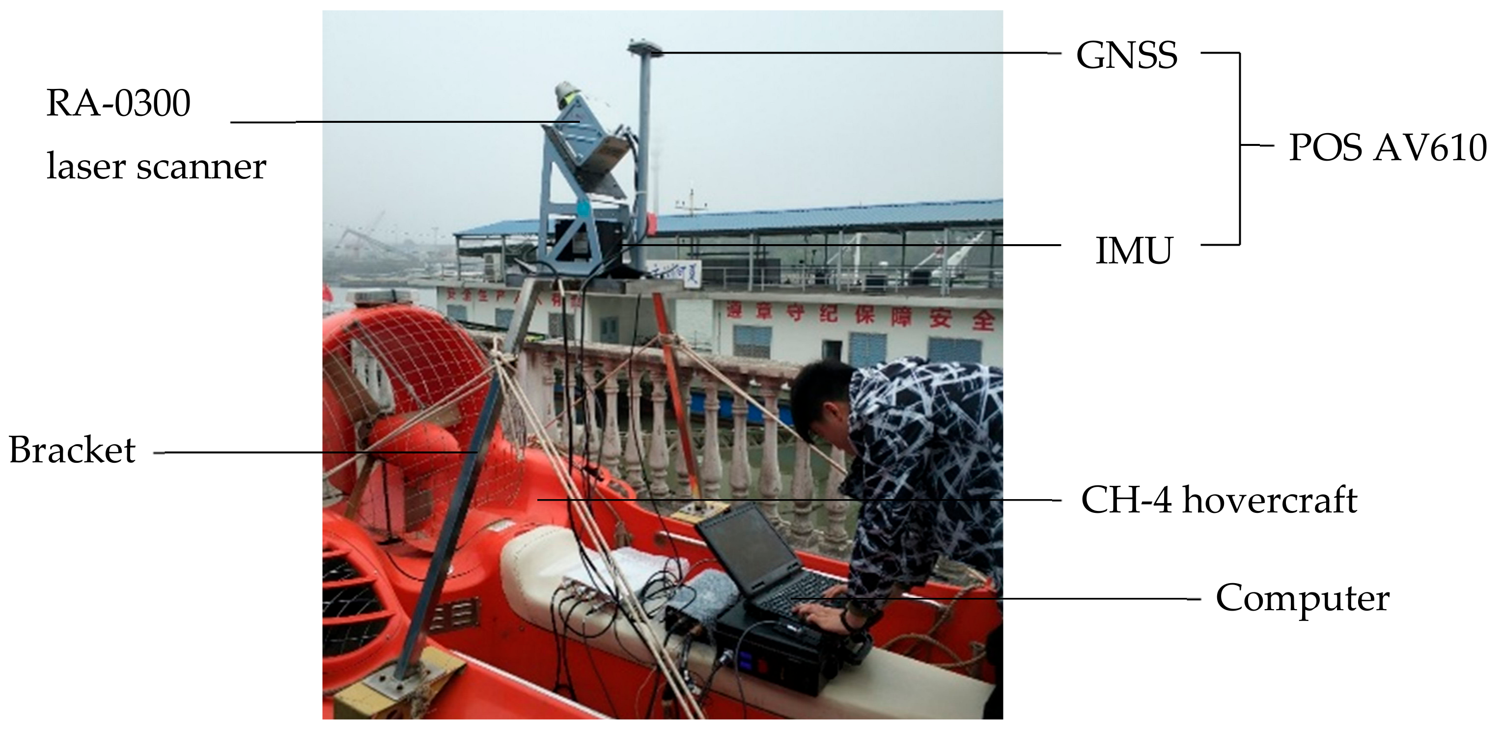
2. Hovercraft-Borne LiDAR System

A hovercraft-borne LiDAR system was designed according to the special environment of mudflats. The system consisted of a CH-4 hovercraft, a SureStar RA-0300 laser scanner, an APPLANIX POS AV610 position and orientation system (POS), a designed bracket, a data acquisition and processing unit (a portable computer), etc. The CH-4 hovercraft was the carrier platform of the mobile mapping system, and the designed bracket fixed on the hovercraft was the equipment support platform. The POS consisted of an IMU (inertial measurement unit) and a GNSS antenna. On the support platform, the scanner, IMU, and GNSS antenna were fixed for obtaining the scanning points, attitudes, and positions during the scanning period, respectively. The integrated mapping system is shown in Figure 1, and the specifications of the main equipment are shown in

Table 1. Specifications of the main equipment.

Equipment	Specification	Accuracy/Range	Specification	Accuracy/Range
R-Angle 0300 Laser Scanner	Min. Range (m)	1.5	Field of View (°)	360
	Max. Range (m)	600	Echoes	Multiple
	Max. Pulse Frequency (kHz)	1000	Wavelength (nm)	1550
	Scan Speed (Hz)	10–200	Scanner Weight (kg)	<5
	Beam Divergence (mrad)	<0.35	Power Supply (V DC)	18–32
	Angle Resolution (°)	0.001	Power Consumption (W)	<100
	Angle Precision (°)	0.005	Storage Temperature (℃)	−35 to 70
	Range Precision (mm @ 100 m)	5–8	Operation Temperature (℃)	−20 to 65
APPLANIX POS AV610	GNSS Position (m)	0.05–0.3	Roll and Pitch (°)	0.0025
	Velocity (m/s)	0.005	True Heading (°)	0.005
CH-4 Hovercraft	Size (m)	4.6 × 2.4 × 1.65	Hover Height (mm)	≤220
	Weight (kg)	380 ± 50	Speed (mud/sand) (km/h)	30–45

. Table 1 indicates that the hovercraft could travel at a speed of 30–45 km/h on the mudflat surface, guaranteeing a high-efficiency survey.

The designed stainless-steel bracket was an isosceles trapezoid with 2.2 m baseline and 1.8 m height. The top rectangle surface of the bracket was 0.6 m × 0.4 m. The rubber mat, IMU, scanner and GNSS antenna were fixed from bottom to top, respectively. The coordinates of the laser scanner and the GNSS antenna in IMU reference coordinate system and the rotation angles between the three axes of the laser scanner reference coordinate system and the IMU reference coordinate system were calibrated in the calibration field. The observation equipment were powered by storage batteries. These observation data were connected to the portable computer for storage and processing by their respective communication cables. To guarantee accurate measurement, GNSS RTK/PPK positioning technology was adopted in the mobile mapping system. Generally, a GNSS reference station needs to be set up at the control point, and the height of GNSS antenna is also required. During the measurement, the sampling frequencies of GNSS, IMU, and laser scanner were set to 20 Hz, 200 Hz, and 200 kHz, respectively. The positions of the GNSS antenna were obtained by RTK/PPK technology with centimeter-level accuracy, and they provided the absolute reference for the instantaneous absolute coordinate calculation of the point cloud.

3. Ground Points Acquisition

3.1. Data Synchronization

In the integrated system, the absolute geographic positions came from the GNSS and were labelled with UTC time while the attitude data from IMU and the laser scanning data were labelled with computer time after being input into the computer. Only when the synchronization was performed could the absolute coordinates of points be obtained by combining the above observation data [6]. Two schemes could perform the synchronization. The first scheme adopted GNSS 1 PPS (pulse per second) technology to send pulse signals to the IMU and the scanner, and get attitude data and laser scanning data with UTC time labels. The second scheme carried out the synchronization by software. The software received GNSS NMEA0183 messages, laser scanning data, and attitude data, sent them to the computer, and labelled them with computer time. The NMEA0183 message contained UTC time, so according to the computer time and UTC time of the same NMEA0183 message, the time deviation could be calculated as:

$${\mathsf{\Delta }\mathit{T}}_{\mathit{i}}^{\mathrm{C}-\mathrm{UTC}} ={ \mathit{T}}_{\mathit{i}}^{\mathrm{C}} -{ \mathit{T}}_{\mathit{i}}^{\mathrm{UTC}},$$

(1)

where ΔT^C-UTC is the time deviation between computer time T^C and UTC time T^UTC. With the time deviation, UTC time could be transformed to computer time, and thus the synchronizations among GNSS positions, attitude data, and laser scanning data could be realized.

Because of the difference of sampling rate, the above three kinds of measurement data were not aligned. To align these data, a linear interpolation was adopted. Firstly, the positions from GNSS and the attitudes from IMU could be aligned using an integrated navigation algorithm [31], and then the positions and attitudes could be interpolated to match the scanning data. The interpolation model is expressed as:

$${\mathit{X}}_{\mathit{i}} ={ \mathit{X}}_{\mathit{j}} + \frac{{\mathit{X}}_{\mathit{j}+1 }-{ \mathit{X}}_{\mathit{j}}}{{\mathit{T}}_{\mathit{j}+1} -{ \mathit{T}}_{\mathit{j}}}{(\mathit{T}}_{\mathit{i}} -{ \mathit{T}}_{\mathit{j}}),$$

(2)

where X is the position or attitude value, T_i is the time to be interpolated, T_j and T_j+1 are the time of the jth and the j+1th position or attitude values, and T_j ≤ T_i ≤ T_j+1.

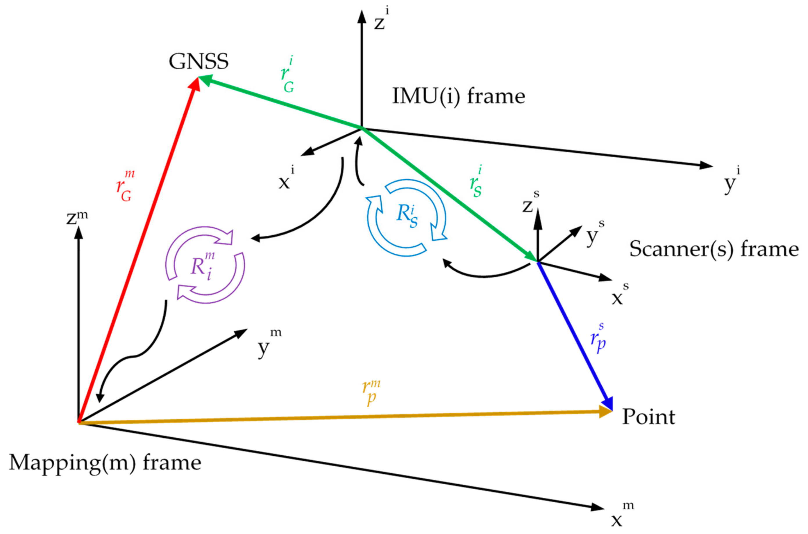
3.2. Coordinate Calculation of Laser Points

The coordinate calculation principle of the laser points is shown in Figure 2.

In Figure 2, (xyz)^s, (xyz)^I, and (xyz)^m represent the three axes of the scanner frame, IMU frame, and mapping frame (usually geographic reference coordinate system), respectively; ${\mathit{r}}_{\mathit{p}}^{\mathit{m}}$, ${\mathit{r}}_{\mathit{G}}^{\mathit{m}}$, ${\mathit{r}}_{\mathit{p}}^{\mathit{s}}$, ${\mathit{r}}_{\mathit{s}}^{\mathit{i}}$, and ${\mathit{r}}_{\mathit{G}}^{\mathit{i}}$ represent the five coordinate vectors of the scanning point in the mapping frame, the GNSS center in the mapping frame, the scanning point in the scanner frame, the scanner center in the IMU frame, and the GNSS center in the IMU frame, respectively; ${\mathit{R}}_i^{\mathit{m}}$ and ${\mathit{R}}_s^{\mathit{i}}$ represent the rotation matrixes from the IMU frame to the mapping frame and from the scanner frame to the IMU frame. Among them, ${\mathit{r}}_{\mathit{p}}^{\mathit{m}}$ is the point cloud coordinate to be calculated; ${\mathit{R}}_{\mathit{s}}^{\mathit{i}}$, ${\mathit{r}}_{\mathit{s}}^{\mathit{i}}$, and ${\mathit{r}}_{\mathit{G}}^{\mathit{i}}$ are obtained after system installation and calibration; ${\mathit{r}}_{\mathit{p}}^{\mathit{s}}$ is calculated by the range and angle measured by the laser scanner; ${\mathit{R}}_{\mathit{i}}^{\mathit{m}}$ is provided by the IMU; and ${\mathit{r}}_{\mathit{G}}^{\mathit{m}}$ is provided by the GNSS.

The point cloud coordinates are [32]:

$${\mathit{r}}_{\mathit{p}}^{\mathit{m}} = {\mathit{r}}_{\mathit{G}}^{\mathit{m}} + {\mathit{R}}_{\mathit{i}}^{\mathit{m}} ({\mathit{R}}_{\mathit{s}}^{\mathit{i}}{\mathit{r}}_{\mathit{p}}^{\mathit{s}} + {\mathit{r}}_{\mathit{s}}^{\mathit{i}} - {\mathit{r}}_{\mathit{G}}^{\mathit{i}}).$$

(3)

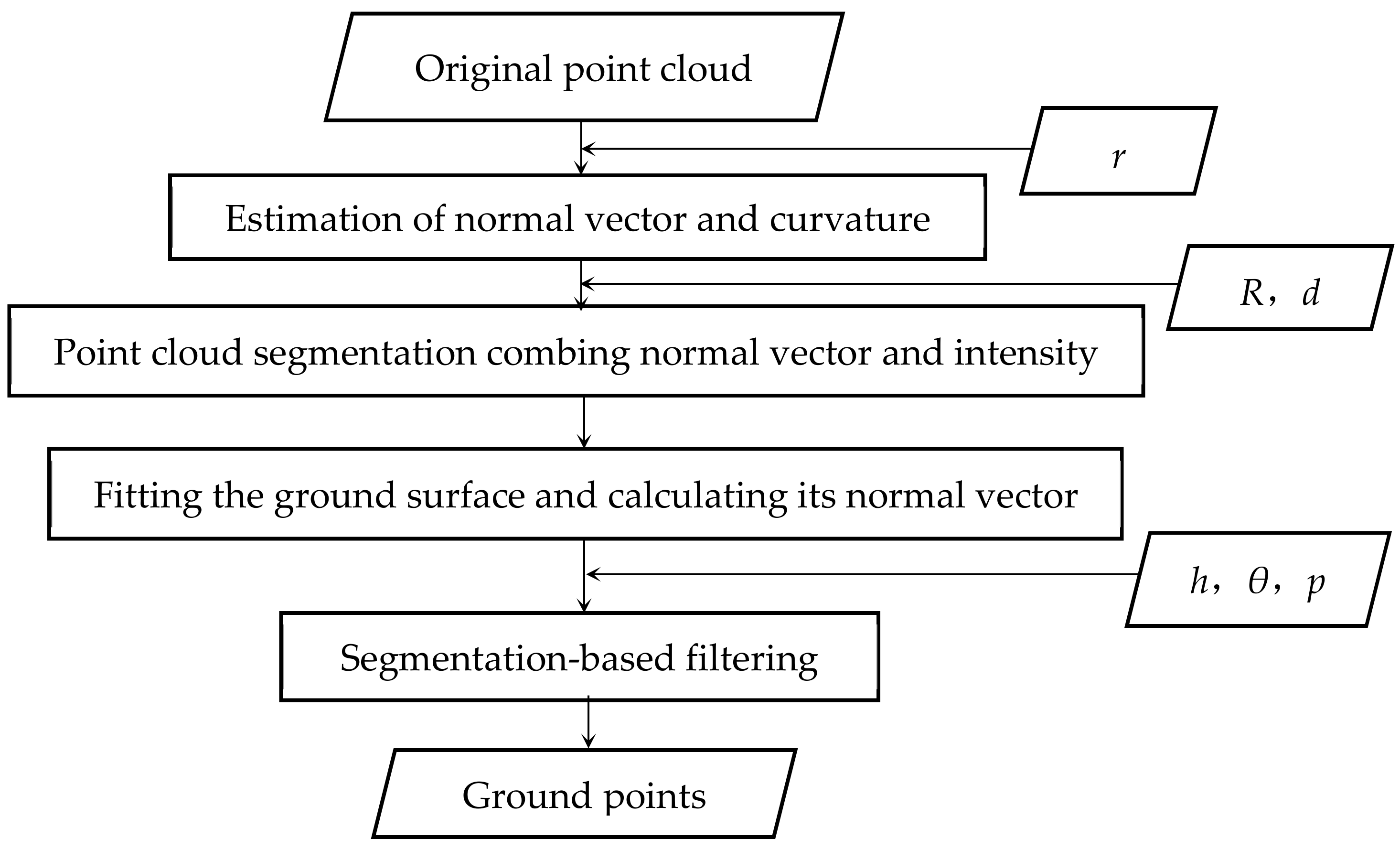
3.3. Comprehensive Filtering of the Point Cloud

In order to obtain the point cloud that describes the mudflat topography, a comprehensive filtering method is illustrated in this section. Firstly, the method combines the normal vectors and intensities of points to segment the point cloud into different segments by a region-growing algorithm; secondly, it calculates the fitting surface of the ground using a cloth simulation algorithm; finally, it synthetically judges the ground points by combining the distance of the point to the fitting surface, the angle difference between the normal vectors of the point and the fitting surface, and the proportion of the possible ground points in the total points of each segment.

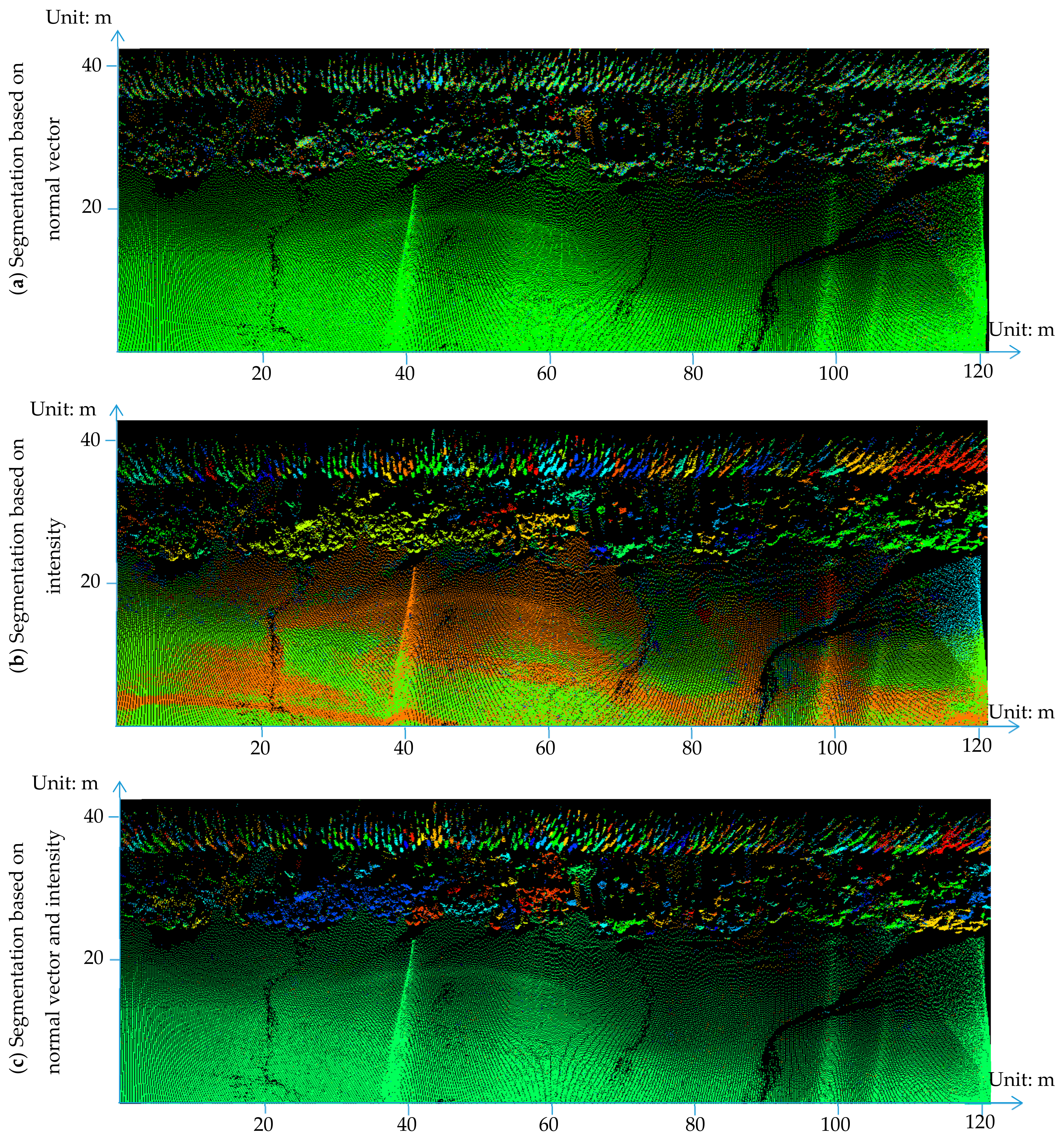
3.3.1. Point Cloud Segmentation by Combining Normal Vector and Intensity

The region-growing-based segmentation algorithm is a classic point cloud segmentation algorithm. Starting from seed points, the method realizes point cloud segmentation by merging neighboring points with similar attributes (e.g., normal vector or intensity, color, curvature, etc.) [33]. Zhan and Liang [34] presented a discriminating criterion in region growing. The criterion uses the unitized three-dimensional normal vector and normalized RGB color values of the point to build the six-dimensional attribute vector of the point. According to the Euclidean distance of the six-dimensional attribute vectors between the seed point and the candidate point, the similarity of the attributes between points is judged, and then it is determined whether the candidate point and the seed point belong to the same segment. Based on this concept, considering the intensity differences among different objects, this paper proposes to build the four-dimensional attribute vector A (Equation (4)) using the unitized three-dimensional normal vector and normalized intensity value of the point to perform the segmentation by region growing. In addition, in order to improve the computational efficiency, the Euclidean distance is replaced by the Taxi distance (Equation (5)) when calculating the distance between attribute vectors of points. Finally, the point cloud segmentation is realized by setting the distance threshold in the region growing. The proposed method is detailed as follows:

• For each point, its normal vector and curvature are estimated using the points within radius r to fit a local surface. The unitized normal vector and normalized intensity value are used to build a four-dimensional attribute vector A:

  A = [ N_x N_y N_z I ],

  (4)

  where N_x, N_y, and N_z are the normal vector components in the directions of x, y, and z, and N_x² + N_y² + N_z² = 1; I is the intensity value of the point within the range 0–1 after normalization.
• Among all points, the point with the minimum curvature is selected as a seed point P₀, and a new segment O is generated. P₀ is included in O and marked as a segmented point.
• The points around P₀ within the radius R are searched as candidate points. For each candidate point P_i, the distance ${\mathit{D}}_{\mathrm{taxi}}^{0\mathit{i}}$ between the attribute vectors of P_i and P₀ is calculated by Equation (5):

  $${\mathit{D}}_{\mathrm{taxi}}^{0\mathit{i}}{ = |\mathit{N}}_{\mathrm{x}}^0 -{ \mathit{N}}_{\mathrm{x}}^{\mathit{i}}{| + |\mathit{N}}_{\mathrm{y}}^0 -{ \mathit{N}}_{\mathrm{y}}^{\mathit{i}}{| + |\mathit{N}}_{\mathrm{z}}^0 -{ \mathit{N}}_{\mathrm{z}}^{\mathit{i}}| + 2\sqrt{3}{|\mathit{I}}^0 -{ \mathit{I}}^{\mathit{i}}|,$$

  (5)

  where ${\mathit{N}}_{\mathrm{x}}^0$(${\mathit{N}}_{\mathrm{y}}^0$/${\mathit{N}}_{\mathrm{z}}^0$/${\mathit{I}}^0$) and ${\mathit{N}}_{\mathrm{x}}^{\mathit{i}}$(${\mathit{N}}_{\mathrm{y}}^{\mathit{i}}$/${\mathit{N}}_{\mathrm{z}}^{\mathit{i}}$/${\mathit{I}}^{\mathit{i}}$) represent the N_x(N_y/N_z/I) in the A of P₀ and P_i, respectively.
• The threshold d is set in the region growing. Whether or not the candidate point is in O is judged based on the following principle:

  $$\mathrm{if} \begin{array}{c}{\mathit{D}}_{\mathrm{taxi}}^{0\mathit{i}} > \mathit{d}\\ {\mathit{D}}_{\mathrm{taxi}}^{0\mathit{i}} \le \mathit{d}\end{array} \mathrm{then} \begin{array}{c}{\mathit{P}}_{\mathit{i}} \mathrm{is} \mathrm{not} \mathrm{included} \mathrm{in} \mathbf{O},\\ {\mathit{P}}_{\mathit{i}} \mathrm{is} \mathrm{included} \mathrm{in} \mathbf{O}.\end{array}$$

  (6)

  If P_i is included in O, it is marked as a segmented point and becomes a seed point.
• Repeating (4), all the seed points around P₀ within the radius R are found and marked as segmented points.
• By region growing, the new seed points are further found by repeating (3)–(5) and are marked as segmented points until no new point is found and marked. These seed points are all included in O. Then the segment O is segmented completely.
• In the remaining unsegmented points, we can also find the point with the minimum curvature. By following (2)–(6), a new segment is generated. Similarly, we can obtain other segments by repeating (2)–(6) until all the points are segmented.

3.3.2. Fitting the Ground Surface and Calculating Its Normal Vector

The CSF algorithm presented by Zhang et al. [22] simulates a piece of cloth with certain rigidness covering an upside-down point cloud, and the shape of the cloth can be considered as an approximation of the ground surface (Figure 3a). The CSF algorithm has the advantages of high ground-fitting accuracy and only a few easy-to-set parameters [22], so it was used to fit the ground surface in this paper. In the CSF algorithm, the cloth is represented by grid nodes with a certain spacing, so the whole area can be considered as consisting of many small planes (Figure 3b). A plane can be fitted by the four nodes of each mesh. The plane and its normal vector represent the ground surface and its normal vector of the region.

3.3.3. Segmentation-Based Point Cloud Filtering

In traditional surface-based and point-based filtering algorithms, it is easy to mistakenly classify very low object points as ground points based only on the criterion that the distance between the point and the fitting surface is less than the threshold h [28]. As shown in Figure 4, comparing θ₁ with θ₂, it can be found that the angle between the normal vectors of a ground point and the fitting surface is usually smaller, while the angle between the normal vectors of an object point and the fitting surface is larger, which can reduce the situation where very low object points are mistakenly classified as ground points. However, the estimation of normal vectors at the junction of objects is prone to inaccuracy. Taking the point P as an example, its red dotted arrow is the ideal normal vector, and its red solid arrow is the estimated normal vector, which is inaccurate since the neighboring ground points are also involved in the estimation. Adding the judgment of angle is helpful, but cannot completely eliminate the misjudgment. Segmentation-based filtering takes the segment as a whole, so the filtering results of points belonging to the same segment are consistent, which can avoid the misjudgment. Therefore, this paper proposes a modified segmentation-based filtering method, detailed as follows:

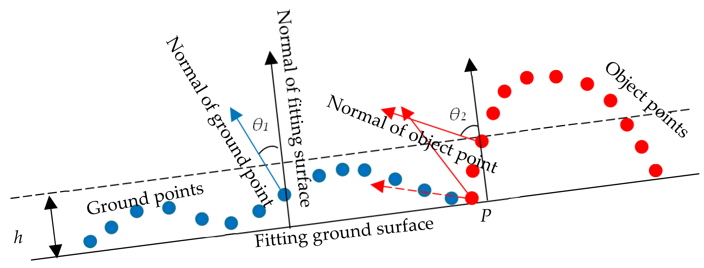
• For each segment, the points belonging to the segment are diagnosed as possible ground points by the following criteria:

  •

  The distance from a diagnosed point to the fitting surface is less than the given threshold h.

  •

  The angle between the normal vectors of the point and the fitting surface is less than the given threshold θ.

• For each segment, the proportion of the possible ground points in the total points of the segment is calculated. If the proportion is higher than the given threshold p, the segment is judged as a ground segment, and all the points belonging to the segment are judged as ground points; otherwise, they are judged as non-ground points.

3.3.4. The Comprehensive Point Cloud Filtering Process

A summary of the process of the comprehensive segmentation-based filtering algorithm is depicted in Figure 5.

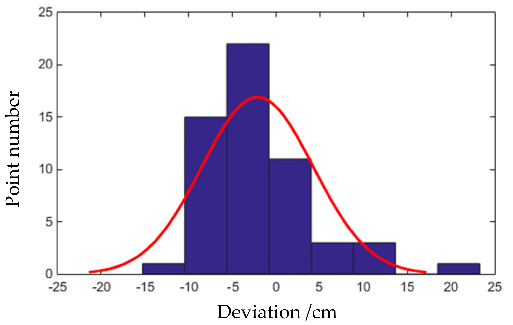
3.4. Accuracy Assessment

The Type I Error (E.I), Type II Error (E.II), and Total Error (E.T) defined by the ISPRS (International Society for Photogrammetry and Remote Sensing) were used to evaluate the filtering accuracy [24]. E.I is the number of ground points that are incorrectly classified as objects points divided by the true number of ground points; E.II is the number of object points that are incorrectly classified as ground points divided by the true number of object points; and E.T is the number of mistakenly classified points divided by the number of total points.

$$\mathrm{E}.\mathrm{I} = \frac{{{n}}_0}{{\mathit{N}}_{\mathit{g}}}, \mathrm{E}.\mathrm{II} = \frac{{\mathit{n}}_{\mathit{g}}}{{\mathit{N}}_{\mathit{o}}}, \mathrm{E}.\mathrm{T} = \frac{{\mathit{n}}_0{ + \mathit{n}}_{\mathit{g}}}{{\mathit{N}}_{\mathit{g}}{ + \mathit{N}}_{\mathit{o}}},$$

(7)

where n_o and n_g are respectively the number of ground points that are incorrectly classified as objects points and the number of object points that are incorrectly classified as ground points; N_g and N_o are respectively the true numbers of ground points and object points.

The absolute elevation accuracy of ground points is evaluated by the statistical result of the elevation differences between RTK ground points and filtered ground points:

$$\mathsf{\sigma } = \sqrt{({{\displaystyle \sum }}_{\mathit{i}=1}^{\mathit{n}}{\left({\mathit{H}}_{\mathit{i}}^{\mathit{g}} -{ \mathit{H}}_{\mathit{i}}^{\mathrm{RTK}}\right)}^2) / \mathit{n}},$$

(8)

where σ is the absolute elevation accuracy, n is the number of RTK points involved in the evaluation, and H^g and H^RTK are the elevations of filtered ground points and RTK points, respectively.

4. Experiment and Analysis

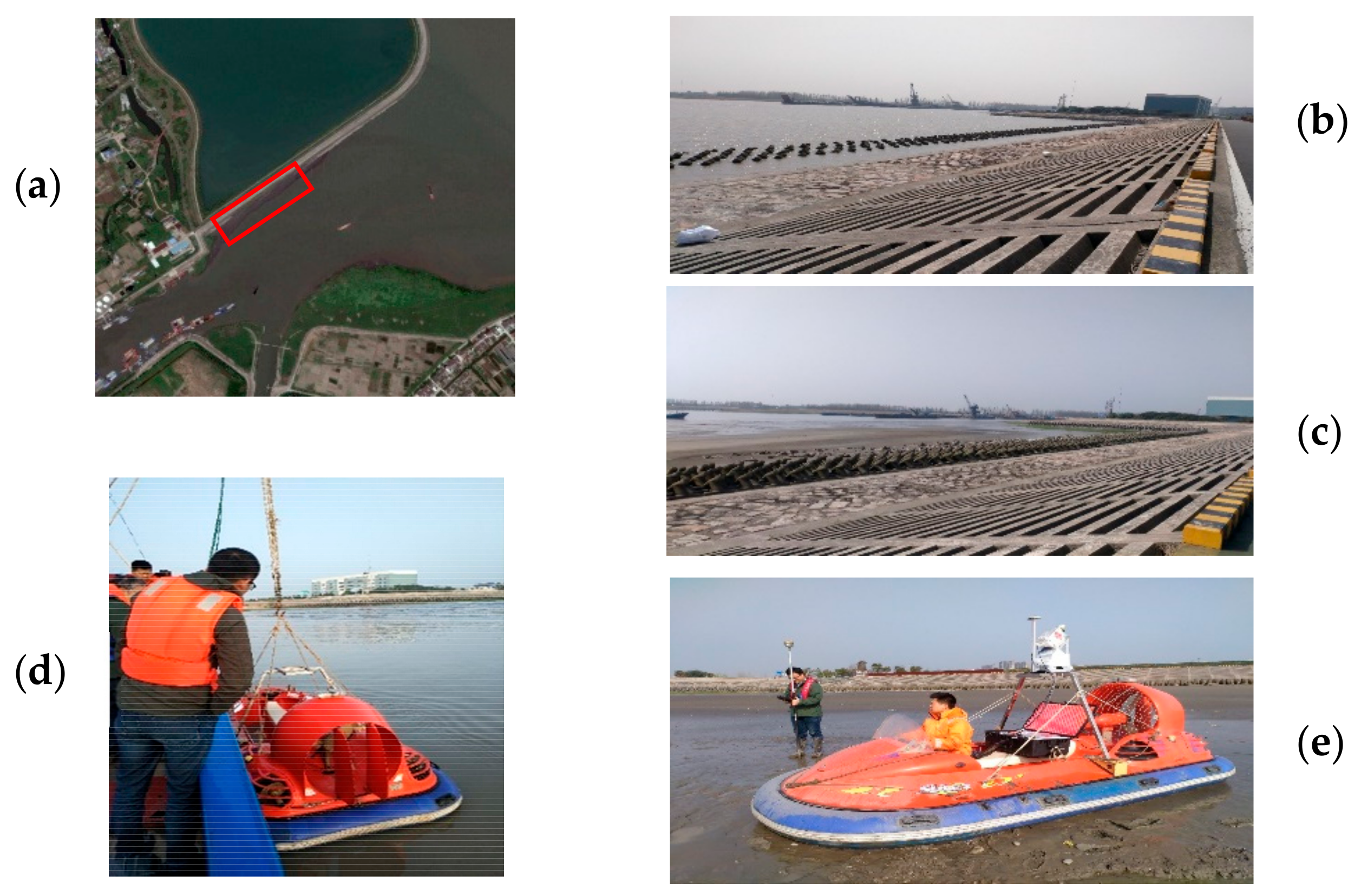
4.1. Overview of the Experiment

In order to verify the effectiveness of the developed system and the proposed filtering method, an experiment was carried out on the mudflat of Liuhe River, Yangtze Estuary, on June 22, 2018 (Figure 6a). The Liuhe River is a tidal river with a maximum tidal range of about 2.8 m. The mudflat is submerged at high tide (Figure 6b) and exposed at low tide (Figure 6c). The main objects on the mudflat are dolosse along the bank, low vegetation, and stones. There are also some ships moored near the low-tide line. Before surveying, a GNSS reference station was set up at a known point near this area. The AV610 POS system was activated, and static observation was carried out for 5 min to ensure the POS’ initialization. The measurement system was transported to the deep-water area and hoisted on the water surface (Figure 6d), then driven to the mudflat area to carry out topographic survey. In order to assess the measurement accuracy of the system, GNSS RTK was also used to collect some ground points. To get a high-accuracy RTK positioning solution, we measured 30 s at each RTK point. Because the mudflat was very soft and broad, only 56 RTK points were measured. However, these points evenly covered about 2/3 of the measured area and were distributed in the topographic gradient direction (Figure 6e and Figure 7c).

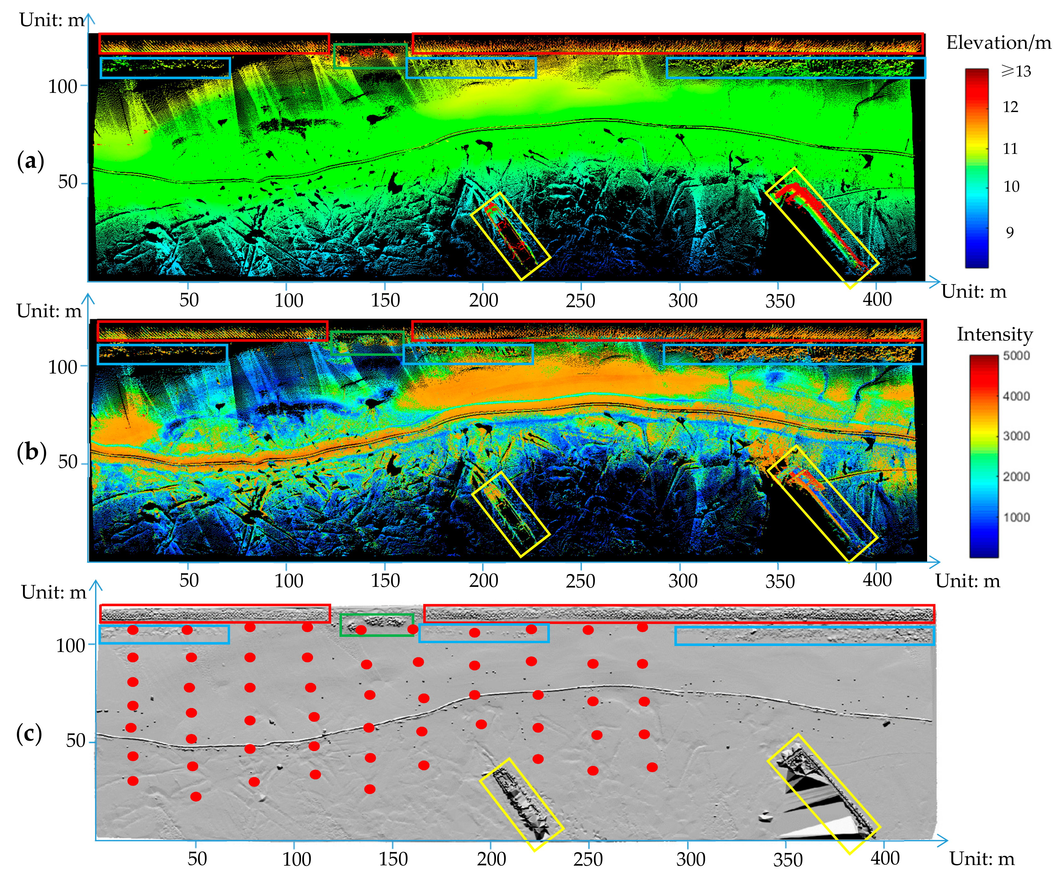
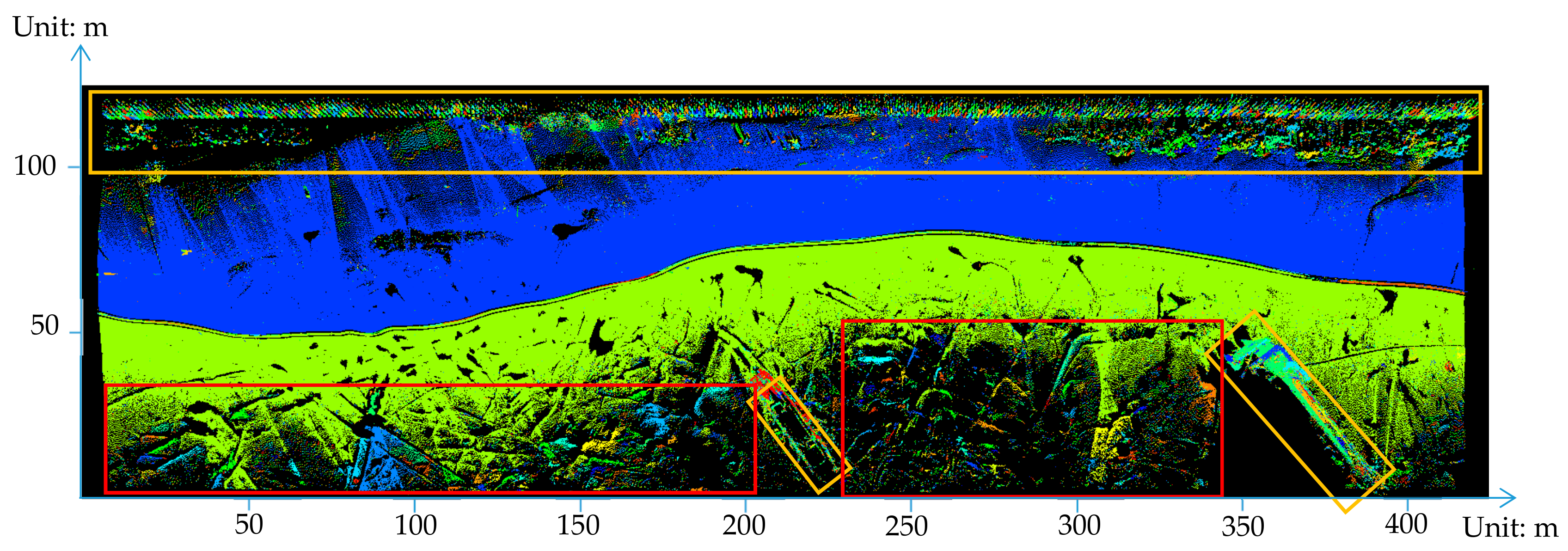
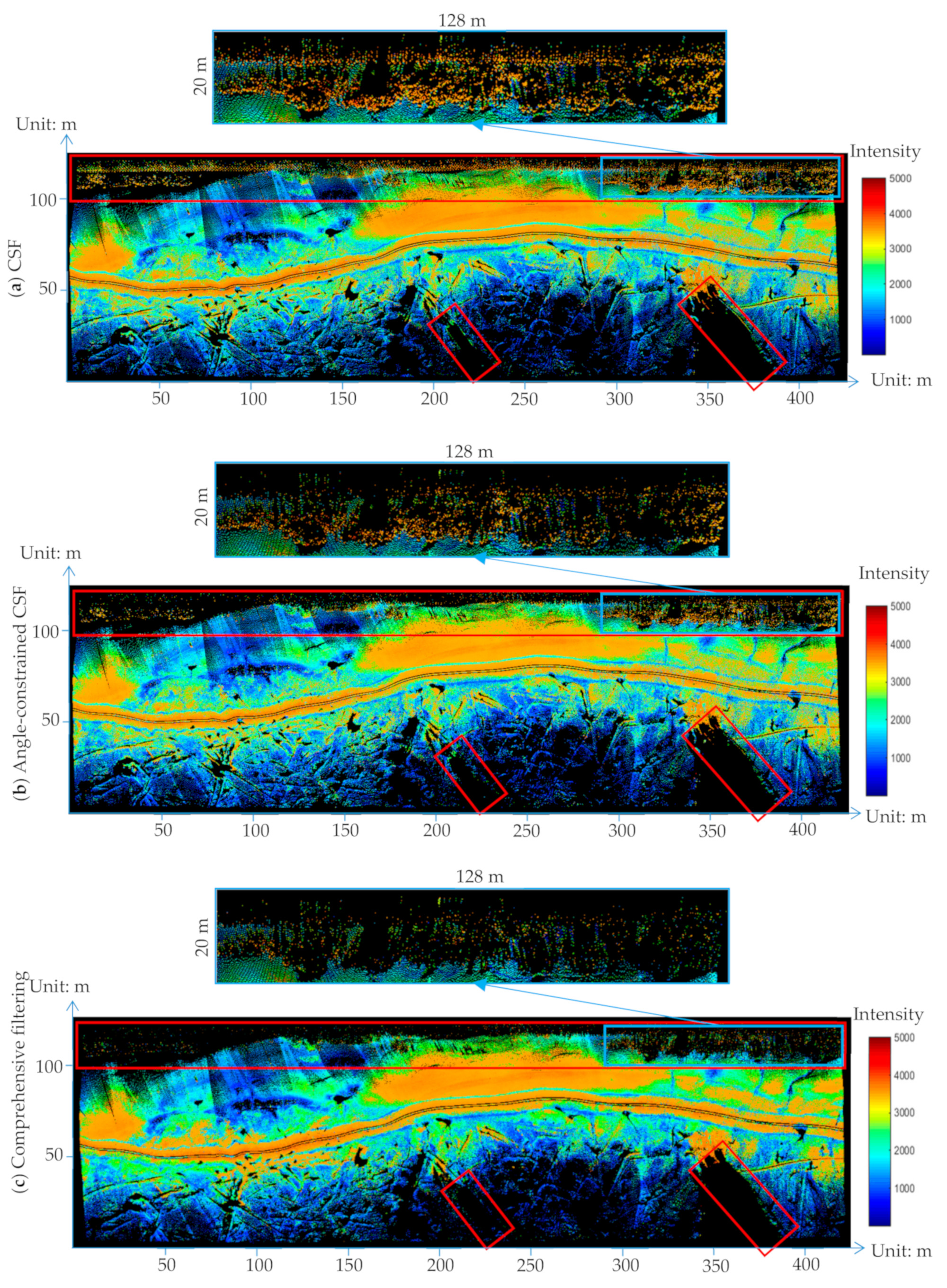
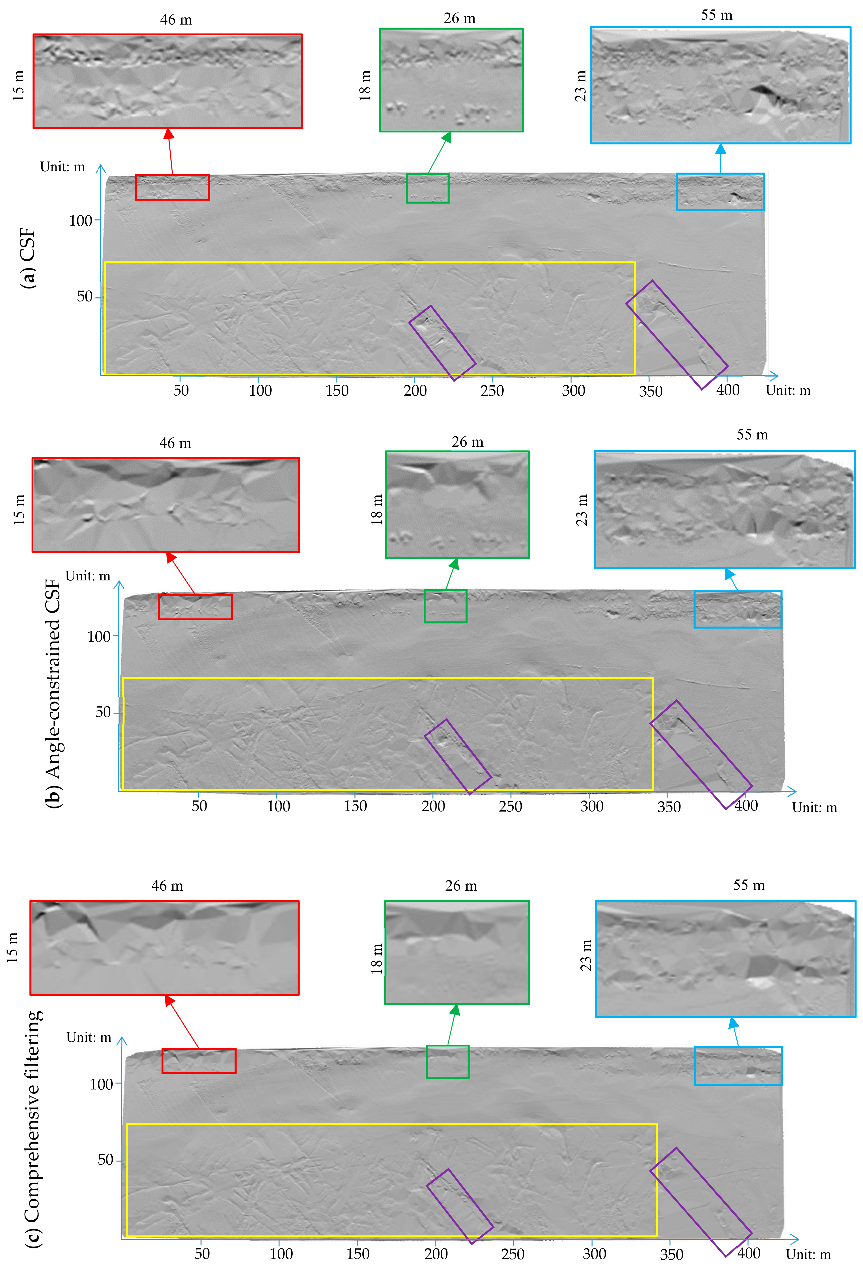
4.2. Data Processing and Analysis

Combining the ranges and angles of laser beams, the attitudes of hovercraft, the positions of GNSS antenna, and the configuration parameters of these sensors on the hovercraft, the 3-D absolute coordinates of each point were calculated according to Equation (3), and the point cloud of this mudflat was obtained as shown in Figure 7. Since the point coordinates were calculated from the GNSS coordinates, the points’ elevations were ellipsoidal heights.

The point cloud contained about 4.3 million points, including the ground and non-ground points. In Figure 7, there are a row of dolosse along the bank, several clusters of vegetation, some stones, and two ships in the red, green, blue, and yellow boxes respectively. The band near the center of the survey area is the track of the hovercraft, and the red points in Figure 7c are RTK points. To obtain the ground points, it was necessary to filter out the non-ground points. The comprehensive filtering algorithm proposed in Section 3.3 was adopted. For comparison, the traditional CSF algorithm and the angle-constrained CSF algorithm were also used in the experiment. The parameters used in the three methods are shown in

Table 2. Parameters used in the three filtering algorithms. CSF: cloth simulation filtering.

Method	Point Cloud Segmentation			Object-Based Filtering
	r (m)	R (m)	d	h (m)	θ (°)	p (%)
Traditional CSF	-	-	-	0.1	-	-
Angle-constrained CSF	-	-	-	0.1	30	-
Comprehensive filtering	0.5	0.5	0.6	0.1	30	75

.

The results of point cloud segmentation are shown in Figure 8. It can be seen that the objects and the ground are separated and shown with different colors, as shown in the orange boxes, which proves the validity of the proposed segmentation algorithm. Although some ground points were over-segmented to some degree due to the large spacing and relief (as shown in the red boxes), these fragments were still classified as ground segments after filtering.

The point cloud results of the three filtering methods are shown in Figure 9. To see more clearly, we zoomed in on a typical area. From the red and blue boxes in Figure 9a, it can be seen that the traditional CSF method could not filter out low object points, so there were still a large number of high-intensity object points. From those of Figure 9b, it can be seen that the angle-constrained CSF improved the traditional CSF with a single distance constraint, although some high-intensity stone points still could not be filtered out. This means that the constraint of normal angle difference was helpful to some extent. Segmentation-based filtering was necessary to further solve the problem of filtering low object points. From those of Figure 9c, it can be seen that the low object points were filtered out more thoroughly by the segmentation-based filtering.

The DTM (digital terrain model) results of the three filtering methods are shown in Figure 10. To see more clearly, we zoomed in on three typical areas.

If a filtering method is accurate, the non-ground points will be removed correctly while the terrain details will be retained, and the interpolated DTMs of the areas where objects are removed will be smoother due to the use of real ground points. Otherwise, the terrain details will be removed and the interpolated DTMs of the areas where objects are removed will become rough or abnormal due to the residual of non-ground points. First, we compared the DTMs obtained by CSF and the angle-constrained CSF (Figure 10a,b). It can be seen that the DTM obtained by the angle-constrained CSF was smoother, which also proves that the constraint of angle was helpful, but there were still low object points remaining—especially from the DTMs in green and purple boxes. So, the segmentation-based filtering was still needed. Comparing the DTMs obtained by the angle-constrained CSF and the comprehensive filtering (Figure 10b,c), it can be seen that the DTM obtained by the proposed method was smoother, especially in the green and purple boxes, which also proves that the proposed method could filter out low object points more thoroughly. In addition, from the yellow boxes in Figure 10, it can be seen that the proposed method could retain terrain details such as furrows on the mudflat. The characteristics of the filtering results show that the proposed comprehensive filtering method had a superior performance to the two traditional point-based methods.

The point cloud and DTM results above show that the proposed comprehensive segmentation-based filtering method could effectively filter out objects while retaining the mudflat topography details.

Taking the results of manual filtering as reference, the E.I, E.II, and E.T of the three filtering results were calculated by Equation (7) and are shown in

Table 3. The filtering accuracy.

Method	E.I (%)	E.II (%)	E.T (%)
Traditional CSF	0.2	20.1	1.9
Angle-constrained CSF	0.3	10.5	1.3
Comprehensive filtering	0.2	2.8	0.3

. It can be seen that the E.Is of the three methods were similar and small, as the three methods are all based on the CSF method. The CSF method had high surface fitting accuracy and the mudflat was relatively flat, so only a few ground points were judged as object points. In addition, the number of ground points was very large, so the E.I was very small. The E.II of CSF was the largest, because the CSF method took points as filtering elements based on a single h threshold of 0.1 m, and thus incorrectly judged a large portion of the object points close to the ground as ground points. The E.II of the angle-constrained CSF method was smaller than that of CSF, because the angle-constrained CSF added the constraint of normal angle difference between the point and the fitting surface on the basis of CSF, which reduced the misjudgments. However, due to the inaccurate estimation of normal vectors at the junction of objects, misjudgments were still made, and the E.I also increased slightly. In the comprehensive filtering method, the point cloud was first segmented by combining normal vector and intensity, and then the filtering was performed based on the segments, so the low object points were filtered out more thoroughly. Therefore, the E.II of the proposed method was significantly reduced. Based on the E.I and E.II, the E.T obtained by the proposed method was much smaller than that of the two traditional point-based filtering methods, verifying the validity of the proposed method.

To absolutely evaluate the performance of the developed system and the point cloud data processing method, 56 topographic points (Figure 7c) measured by RTK were taken as references. Comparing the elevations of RTK points with those of corresponding positions interpolated by ground points after filtering, 100% of the point elevation deviations were within the range −25 to 25 cm, 90% of those were in the range −10 to 10 cm, and 50% of those were in the range −5 to 5 cm. The statistical results of the deviations (

Table 4. The statistics of elevation deviations between RTK points and laser points.

Max. (cm)	Min. (cm)	Average (cm)	RMSE (cm)
23.0	−15.3	−2.1	6.4

and Figure 11) indicate that the root mean square error (RMSE) of the elevation of the point cloud measured by the developed system was 6.4 cm. There was no obvious systematic error, and the error distribution approximately obeyed a normal distribution. The above results further indicate that the proposed mobile mapping system and comprehensive data processing method can meet the requirements of large-scale topographic mudflat surveys.

5. Discussion

5.1. The Mobile Measuring System

The laser scanner had a scanning scope of 0– 360°, so the hovercraft was included in scans. The laser points from the hovercraft are unnecessary. Therefore, if the range of a laser beam was less than 2 m, the corresponding point was removed, and two blank bands were formed (Figure 12a). In Figure 12a, it can be seen that there were some ground points between the two blank bands. These points were obtained by the laser beams passing through the gap of the propeller and hitting the ground. Because of the two blank bands, the ground points on the two sides of the track were separated into two segmentation results, so they are shown with different colors (Figure 8). To avoid this problem, in the future we could add an inclination to the laser scanner, and then the scanning plane could be kept away from the hovercraft and the ground points under the hovercraft could be scanned. The angle of inclination can be determined by the height of the scanner and the horizontal distance from the scanner to the stern of the hovercraft.

5.2. Obtaining the Mudflat Topography

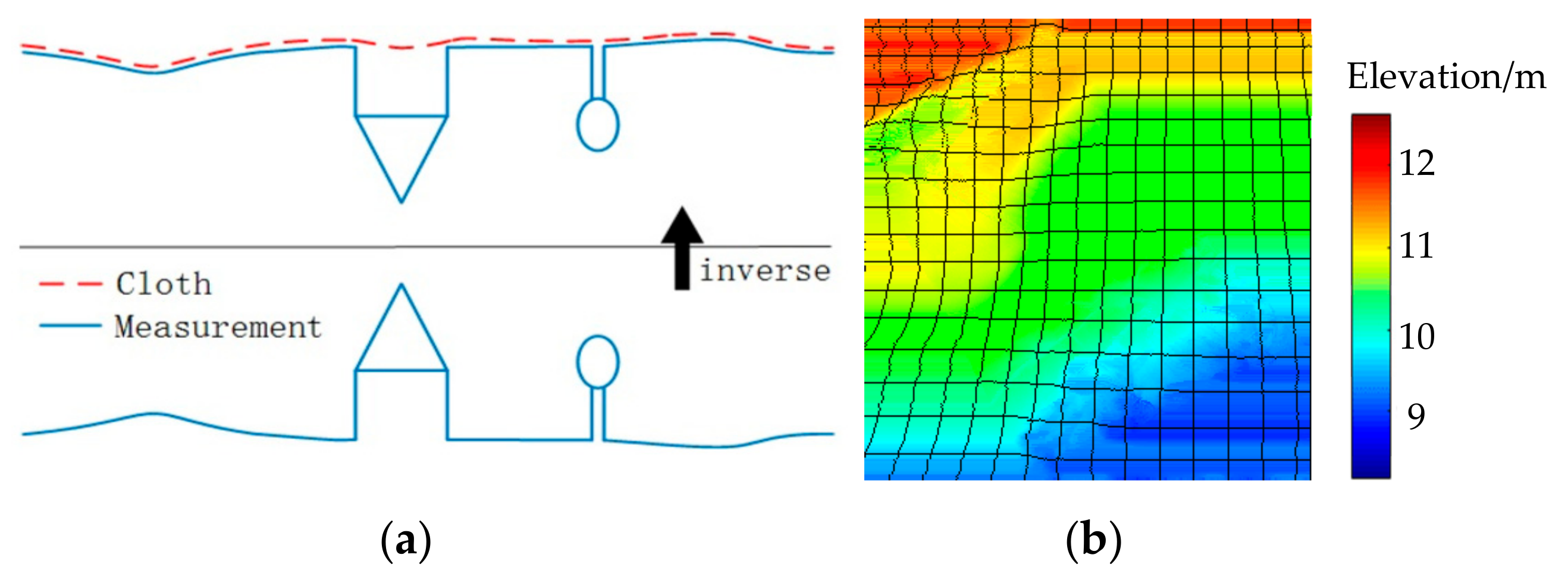
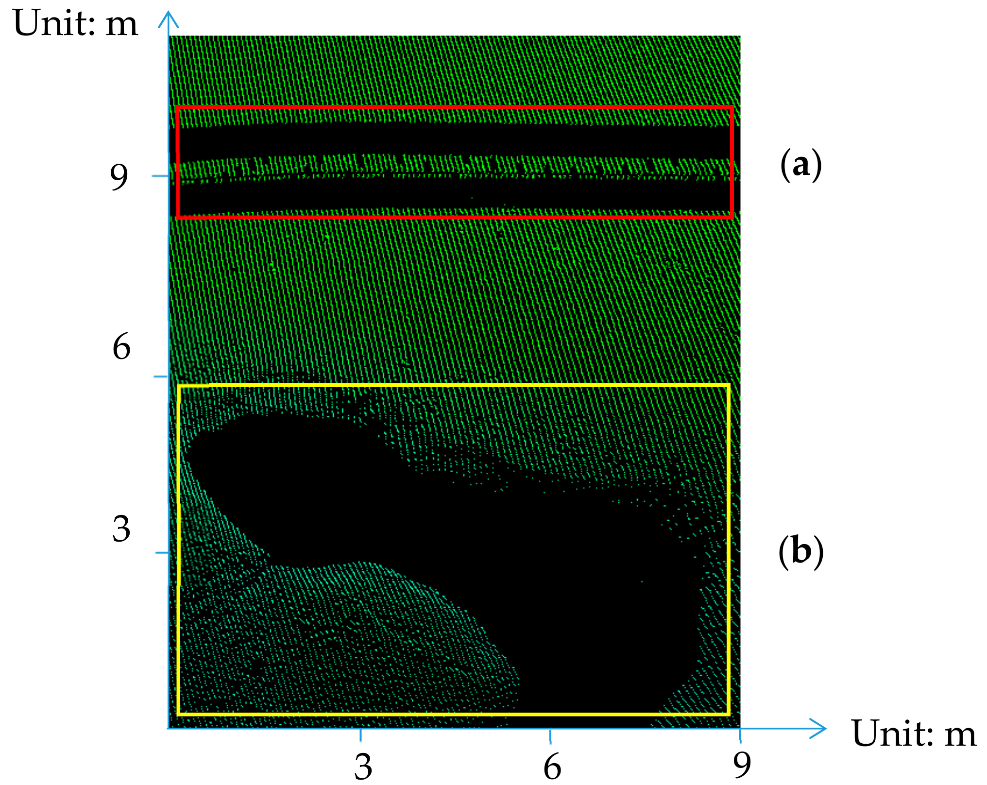
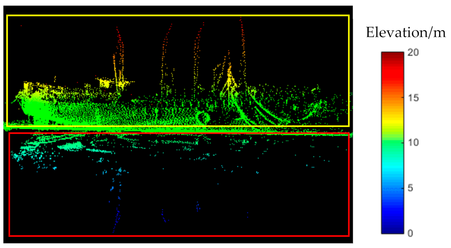
5.2.1. Removal of Outliers Lower than the Mudflat Surface before Filtering

The point cloud measured by LiDAR contained some points that were far higher or lower than the mudflat surface, and we considered these points as outliers. The high outliers can usually be ignored because they can be treated as non-ground objects and filtered out easily. However, the existence of low outliers is one of the circumstances under which the filtering algorithms are likely to fail, especially for the filtering methods based on the assumption that the lowest point in a grid cell must belong to the terrain [24]. The CSF method used in this paper is also sensitive to the low outliers, which should be removed before filtering [22]. In fact, automatic outlier removal is a near-impossible mission because there are various types of errors, such as isolated outliers and clustered outliers [28]. In this paper, there were low outliers in the original point cloud as well. As shown in Figure 13, there were many low outliers (in the red box) below the mudflat surface and these outliers were almost symmetrical with the real ship points (in the yellow box). It can be inferred that these outliers were produced by the multi-path effect. Many low outliers were so close to the mudflat surface that it was difficult to remove them by automatic statistical methods. In this paper, we removed the low outliers manually before filtering, and the automatic removal of low outliers deserves further study in the future.

5.2.2. Point Cloud Segmentation by Combining Normal Vector and Intensity

In this paper, the point clouds were segmented based on region growing by combining normal vector and intensity information, the advantage of which is that it makes up for the shortcomings of segmentation based only on normal vector or intensity. This is illustrated in Figure 14.

Because the estimation of normal vectors at the junctions of objects is prone to inaccuracy, if only the normal vectors are used for segmentation, it is necessary to set a smaller threshold for separating the objects from the ground. In this case, objects will be seriously over-segmented, as shown in Figure 14a. The intensity information can generally distinguish the objects from the ground. However, significant intensity changes also occur on the ground due to the laser range, incident angle, the different degrees of ground humidity, noise, etc. If the segmentation is based only on intensity, the ground point cloud will also be seriously over-segmented, as shown in Figure 14b. By combining the normal vector and intensity, the objects and the ground are separated, but the over-segmentation problem is avoided, and thus a more appropriate segmentation result is obtained (Figure 14c).

In this paper, the normal vector and intensity are given equal weight when calculating the distance between attribute vectors. Based on mathematical principles, we know that |${\mathit{N}}_{\mathrm{x}}^0$ − ${\mathit{N}}_{\mathrm{x}}^{\mathit{i}}$| + |${\mathit{N}}_{\mathrm{y}}^0$ − ${\mathit{N}}_{\mathrm{y}}^{\mathit{i}}$| + |${\mathit{N}}_{\mathrm{z}}^0$ − ${\mathit{N}}_{\mathrm{z}}^{\mathit{i}}$| is within the range of 0–2$\sqrt{3}$ and |${\mathit{I}}^0$ − ${\mathit{I}}^{\mathit{i}}$| is within the range of 0–1, so the coefficient before |${\mathit{I}}^0$ − ${\mathit{I}}^{\mathit{i}}$| in Equation (5) was set to 2$\sqrt{3}$.

5.2.3. Filtering Parameter Setting

The general principle of setting filtering parameters is balancing E.I and E.II as far as possible to reduce the E.T.

In point cloud segmentation, three parameters need to be determined, that is, the neighborhood range r for normal vector estimation, the search radius R, and the distance threshold d for region growing.

The setting of r depends on the spacing of points. In this paper, the spacing between scanning lines was about 0.3 m, so r was set to 0.5 m. This ensured that the neighboring points of the two scanning lines beside each point also participated in the normal vector estimation, and thus a more accurate result could be obtained. If r were less than 0.3 m, the points used in the normal vector estimation would belong to the same scanning line, and the normal vector would be inaccurately estimated.

The size of R is usually slightly larger than the spacing of points, which ensures that the neighboring candidate points can be found. If R is too large, it is easy to cause under-segmentation. According to the spacing of adjacent scanning lines, R was set to 0.5 m in this paper, ensuring that the neighboring points of the adjacent scanning lines could be searched.

The d used in Equation (6) is related to the quality of point cloud segmentation. If d is too large, it is generally prone to under-segmentation, otherwise, the problem of over-segmentation may occur. In the segmentation-based filtering, under-segmentation (i.e., the case where the ground points and object points are not separated) will inevitably cause filtering error, while over-segmentation may not produce this problem because the fragments produced by over-segmentation can still be correctly classified. Therefore, the principle of determining d in this paper was to avoid under-segmentation as far as possible and tolerate a certain degree of over-segmentation. Considering the differences of normal vectors and intensity values among different objects and the experimental results, d was set to 0.6 in this paper.

In the segmentation-based filtering depicted in Section 3.3.2, three parameters need to be determined: the distance threshold h, the angle difference threshold θ, and the proportion threshold p. As shown in Figure 4, h should be set to the relative maximum undulating height of the local topography, and θ should be set to the relative maximum slope of the local topography. Considering the relatively flat mudflat topography and the accuracy requirement (0.1 m) of the elevation survey, in this paper, h was set to 0.1 m and θ was set to 30° in order to retain the ground points. In the traditional object-based filtering algorithm, p is a default value of 50% [25,28], which cannot adapt to complex situations. The setting of p should be flexibly adjusted according to the height of the non-ground objects. In this experiment, there were a large number of low stones. Because many stone points were judged as possible ground points, if p was set to 50%, a large number of stone segments would have been judged as ground segments. To prevent this situation, p should be set to larger than 50%. In this paper, p was set to 75% by experiments. Using this larger p, the vast majority of stone points were filtered out, but the topographic details were retained well.

5.2.4. Interpolation in Blank Areas

There were some blank areas in the point cloud. Besides the blank bands mentioned in Section 5.1, the shield of objects also creates blank areas, as shown in the red boxes of Figure 9c. In addition, water was accumulated in some places on the mudflat, where specular reflection occurred and the laser beams could not get echoes, so blank areas were also generated (Figure 12b). For these blank areas, their elevations could be interpolated by the points around them. The final interpolated DTM is shown in Figure 10c.

6. Conclusions

This paper presents the development of a hovercraft-borne LiDAR system and proposes a novel comprehensive point cloud filtering method to solve the problem that traditional measuring systems and data processing methods are restricted in obtaining the mudflat topography. The developed hovercraft-borne LiDAR system can travel above the mud and water surface, and it is not restricted by bad weather conditions or air traffic control. Therefore, it had better performance in measuring the mudflat topography with shallow water and soft mud. Compared with the existing point cloud segmentation methods based only on the single geometric information, the proposed segmentation method combining the geometric and intensity information improved the accuracy of segmentation. The proposed modified segmentation-based filtering method further improved the filtering performance due to the addition of two new constraints—one is the normal difference between the point and the fitting surface, and the other is the proportion of possible ground points in the total points of each segment. Compared with traditional methods, the non-ground points could be filtered out more thoroughly by the proposed method which takes more information into account, and thus a more accurate mudflat topography could be obtained. In the field experiments, the developed system and these proposed data processing methods achieved a total filtering error of 0.3% and elevation accuracy of 6.4 cm, which verified that the proposed system and methods could provide a new and efficient way of obtaining accurate mudflat topography.

References

1. Zhang, Y.G.; Guan, W.; Li, C.P.; Dong, L.J. A study on the exploitation and the sustainable utilization of marine resources in the Bohai Sea. J. Nat. Resour. 2002, 17, 768–775. [Google Scholar]
2. Lai, Z.L.; Zhang, H.D.; Wan, Y.C.; Yue, Y.C. Applications of airborne LIDAR technology in topographic survey of tidal flat and coastal zone. Hydrogr. Surv. Charting 2008, 28, 37–39. [Google Scholar]
3. Mason, D.C.; Kennett, C.G. Beach topography mapping: A comparison of techniques. J. Coast. Conserv. 2000, 6, 113–124. [Google Scholar] [CrossRef]
4. Lee, J.M.; Park, J.Y.; Choi, J.Y. Evaluation of sub-aerial topographic surveying techniques using total station and RTK-GPS for applications in macrotidal sand beach environment. J. Coast. Res. 2013, 65, 535–540. [Google Scholar] [CrossRef]
5. Gonçalves, J.A.; Henriques, R. UAV photogrammetry for topographic monitoring of coastal areas. ISPRS J. Photogramm. Remote Sens. 2015, 104, 101–111. [Google Scholar] [CrossRef]
6. Wehr, A.; Lohr, U. Airborne laser scanning—An introduction and overview. ISPRS J. Photogram. Remote Sens. 1999, 54, 68–82. [Google Scholar] [CrossRef]
7. Baltsavias, E.P. A comparison between photogrammetry and laser scanning. ISPRS J. Photogramm. Remote Sens. 1999, 54, 83–94. [Google Scholar] [CrossRef]
8. Irish, J.L.; White, T.E. Coastal engineering applications of high-resolution lidar bathymetry. Coast. Eng. 1998, 35, 47–71. [Google Scholar] [CrossRef]
9. Dalloz, L.; Brand, A.; Chiniah, I.; Beaumale, D.; Commun, M. Autonomous area mapping with low cost hovercraft platform. Appl. Mech. Mater. 2015, 799–800, 1102–1106. [Google Scholar] [CrossRef]
10. Kukko, A.; Kaartinen, H.; Hyyppä, J.; Chen, Y. Multiplatform mobile laser scanning: Usability and performance. Sensors 2012, 12, 11712–11733. [Google Scholar] [CrossRef]
11. Vosselman, G. Slope based filtering of laser altimetry data. Int. Arch. Photogramm. Remote Sens. 2000, 33, 935–942. [Google Scholar]
12. Sithole, G. Filtering of laser altimetry data using a slope adaptive filter. Int. Arch. Photogramm. Remote Sens. 2001, 34, 203–210. [Google Scholar]
13. Kilian, J.; Haala, N.; Englich, M. Capture and evaluation of airborne laser scanner data. Int. Arch. Photogramm. Remote Sens. 1996, 31, 383–388. [Google Scholar]
14. Zhang, K.; Chen, S.C.; Whitman, D.; Shyu, M.L.; Yan, J.; Zhang, C. A progressive morphological filter for removing nonground measurements from airborne LIDAR data. IEEE Trans. Geosci. Remote Sens. 2003, 41, 872–882. [Google Scholar] [CrossRef] [Green Version]
15. Chen, Q.; Gong, P.; Baldocchi, D.; Xie, G. Filtering airborne laser scanning data with morphological methods. Photogram. Eng. Remote Sens. 2007, 73, 175–185. [Google Scholar] [CrossRef]
16. Li, Y.; Wu, H.; Xu, H.; An, R.; Xu, J.; He, Q. A gradient-constrained morphological filtering algorithm for airborne LiDAR. Opt. Laser Technol. 2013, 54, 288–296. [Google Scholar] [CrossRef]
17. Pingel, T.J.; Clarke, K.C.; Mcbride, W.A. An improved simple morphological filter for the terrain classification of airborne LiDAR data. ISPRS J. Photogramm. Remote Sens. 2013, 77, 21–30. [Google Scholar] [CrossRef]
18. Mongus, D.; Lukač, N.; Žalik, B. Ground and building extraction from LiDAR data based on differential morphological profiles and locally fitted surfaces. ISPRS J. Photogramm. Remote Sens. 2014, 93, 145–156. [Google Scholar] [CrossRef]
19. Kraus, K.; Pfeifer, N. Determination of terrain models in wooded areas with airborne laser scanner data. ISPRS J. Photogramm. Remote Sens. 1998, 53, 193–203. [Google Scholar] [CrossRef]
20. Axelsson, P. DEM generation from laser scanner data using adaptive TIN models. Int. Arch. Photogramm. Remote Sens. 2000, 33, 111–118. [Google Scholar]
21. Mongus, D.; Žalik, B. Parameter-free ground filtering of LiDAR data for automatic DTM generation. ISPRS J. Photogramm. Remote Sens. 2012, 67, 1–12. [Google Scholar] [CrossRef]
22. Zhang, W.; Qi, J.; Wan, P.; Wang, H.; Xie, D.; Wang, X.; Yan, G. An easy-to-use airborne LiDAR data filtering method based on cloth simulation. Remote Sens. 2016, 8, 501. [Google Scholar] [CrossRef]
23. Yang, B.; Huang, R.; Dong, Z.; Zang, Y.; Li, J. Two-step adaptive extraction method for ground points and breaklines from lidar point clouds. ISPRS J. Photogramm. Remote Sens. 2016, 119, 373–389. [Google Scholar] [CrossRef]
24. Sithole, G.; Vosselman, G. Experimental comparison of filter algorithms for bare-earth extraction from airborne laser scanning point clouds. ISPRS J. Photogramm. Remote Sens. 2004, 59, 85–101. [Google Scholar] [CrossRef]
25. Tóvári, D.; Pfeifer, N. Segmentation Based Robust Interpolation—A New Approach to Laser Data Filtering. In Laser Scanning 2005; International Archives of Photogrammetry, Remote Sensing and Spatial Information Sciences: Enschede, The Netherlands, 2005; Volume 36, pp. 79–84. [Google Scholar]
26. Sithole, G.; Vosselman, G. Filtering of Airborne Laser Scanner Data Based on Segmented Point Clouds. In Laser Scanning 2005; International Archives of Photogrammetry, Remote Sensing and Spatial Information Sciences: Enschede, The Netherlands, 2005; pp. 66–71. [Google Scholar]
27. Yan, M.; Blaschke, T.; Liu, Y.; Wu, L. An object-based analysis filtering algorithm for airborne laser scanning. Int. J. Remote Sens. 2012, 33, 7099–7116. [Google Scholar] [CrossRef]
28. Lin, X.G.; Zhang, J.X. Segmentation-based filtering of airborne LiDAR point clouds by progressive densification of terrain segments. Remote Sens. 2014, 6, 1294–1326. [Google Scholar] [CrossRef]
29. Zhang, J.X.; Lin, X.G.; Liang, X.L. Advances and prospects of information extraction from point clouds. Acta Geod. et Cartogr. Sin. 2017, 46, 1460–1469. [Google Scholar]
30. Liu, X. Airborne LiDAR for DEM generation: Some critical issues. Prog. Phys. Geogr. 2008, 32, 31–49. [Google Scholar]
31. Chen, C.J. The Research on Key Technique of Mobile Mapping System Integration. Ph.D. Thesis, Wuhan University, Wuhan, China, 2013. [Google Scholar]
32. Vaughn, C.R.; Bufton, J.L.; Krabill, W.B.; Rabine, D.L. Georeferencing of airborne laser altimeter measurements. Int. J. Remote Sens. 1996, 17, 2185–2200. [Google Scholar] [CrossRef]
33. Besl, P.; Jain, R. Segmentation through variable-order surface fitting. IEEE Trans. Pattern Anal. Mach. Intell. 1988, 10, 167–192. [Google Scholar] [CrossRef]
34. Zhan, Q.L. Segmentation of LiDAR point cloud based on similarity measures in multi-dimension Euclidean space. In Advances in Computer Science and Engineering; Zeng, D., Ed.; Springer: Berlin, Germany, 2012; Volume 141, pp. 349–357. [Google Scholar]
Figure 1. Hovercraft-borne laser scanning system. GNSS: Global Navigation Satellite System; IMU: inertial measurement unit; POS: position and orientation system.
Remotesensing 11 01646 g001
Figure 2. The model of point coordinate calculation.
Remotesensing 11 01646 g002
Figure 3. Overview of (a) the cloth simulation algorithm and (b) the fitting ground surface.
Remotesensing 11 01646 g003
Figure 4. Segmentation-based filtering.
Remotesensing 11 01646 g004
Figure 5. The process of the comprehensive point cloud filtering.
Remotesensing 11 01646 g005
Figure 6. (a) The test mudflat zone (b) during high tide, (c) during low tide. (d) Lifting the equipment; (e) Topographic survey.
Remotesensing 11 01646 g006
Figure 7. Point clouds of the area: (a) 3-D point cloud; (b) Intensity point cloud; (c) The DSM (digital surface model) and Real-Time Kinematic (RTK) points (Red points).
Remotesensing 11 01646 g007
Figure 8. The point cloud segmentation results. Black denotes the background, which means there were no points in these areas. There were about 130,000 segments after segmentation, and each segment is shown with one color.
Remotesensing 11 01646 g008
Figure 9. The point cloud results obtained by the three filtering methods: (a) by CSF; (b) by angle-constrained CSF; and (c) by comprehensive filtering.
Remotesensing 11 01646 g009
Figure 10. The DTM (digital terrain model) results of the three filtering methods: (a) by CSF; (b) by angle-constrained CSF; and (c) by comprehensive filtering.
Remotesensing 11 01646 g010
Figure 11. The distribution of elevation deviations between RTK points and laser points.
Remotesensing 11 01646 g011
Figure 12. Blank areas: (a) formed due to the shield of the hovercraft; (b) produced because of the specular reflection of water.
Remotesensing 11 01646 g012
Figure 13. An example of low outliers.
Remotesensing 11 01646 g013
Figure 14. Comparison of the three segmentation methods: (a) based only on normal vector; (b) based only on intensity; (c) based on the combination of normal vector and intensity.
Remotesensing 11 01646 g014