Evaluation of Four Atmospheric Correction Algorithms for GOCI Images over the Yellow Sea

 , , , ,
Abstract
1. Introduction
2. Algorithms
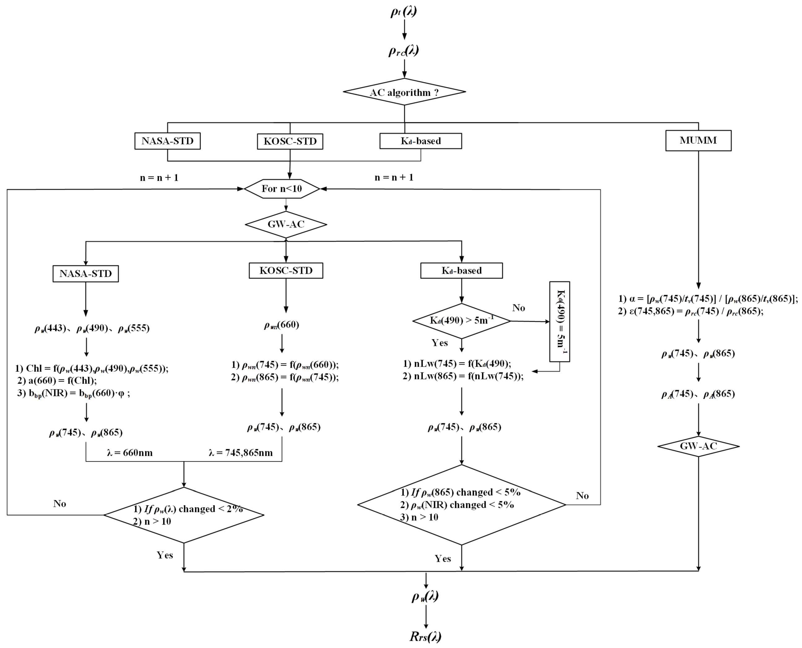
2.1. AC Algorithms
2.1.1. NASA Standard Algorithm (NASA-STD)
2.1.2. KOSC Standard Algorithm (KOSC-STD)
2.1.3. Kd-Based NIR Correction Algorithm (Kd-Based)
2.1.4. MUMM Algorithm
2.2. Chla Retrievals
3. Data and Methods
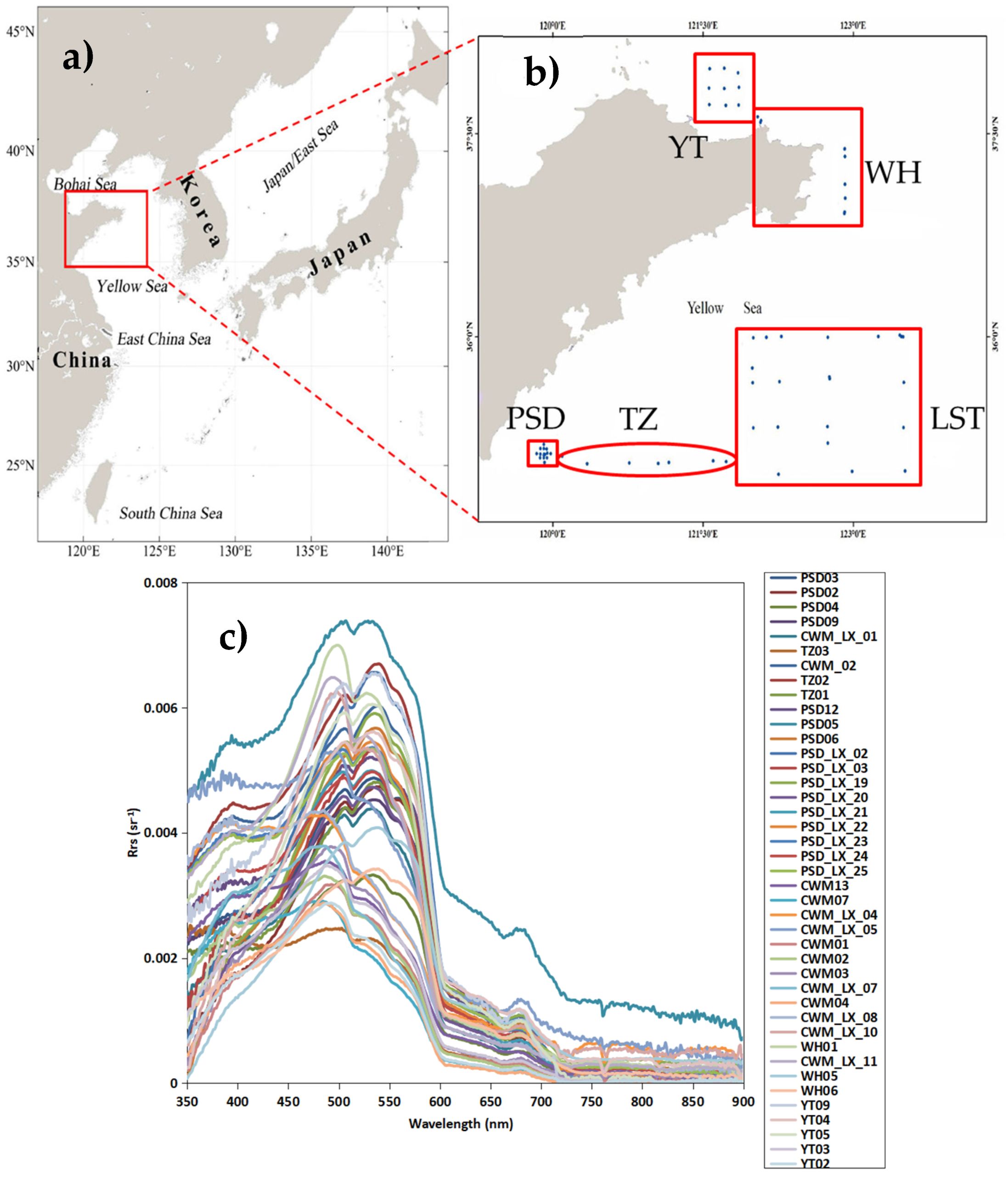
3.1. Study Area
3.2. In Situ Measurements
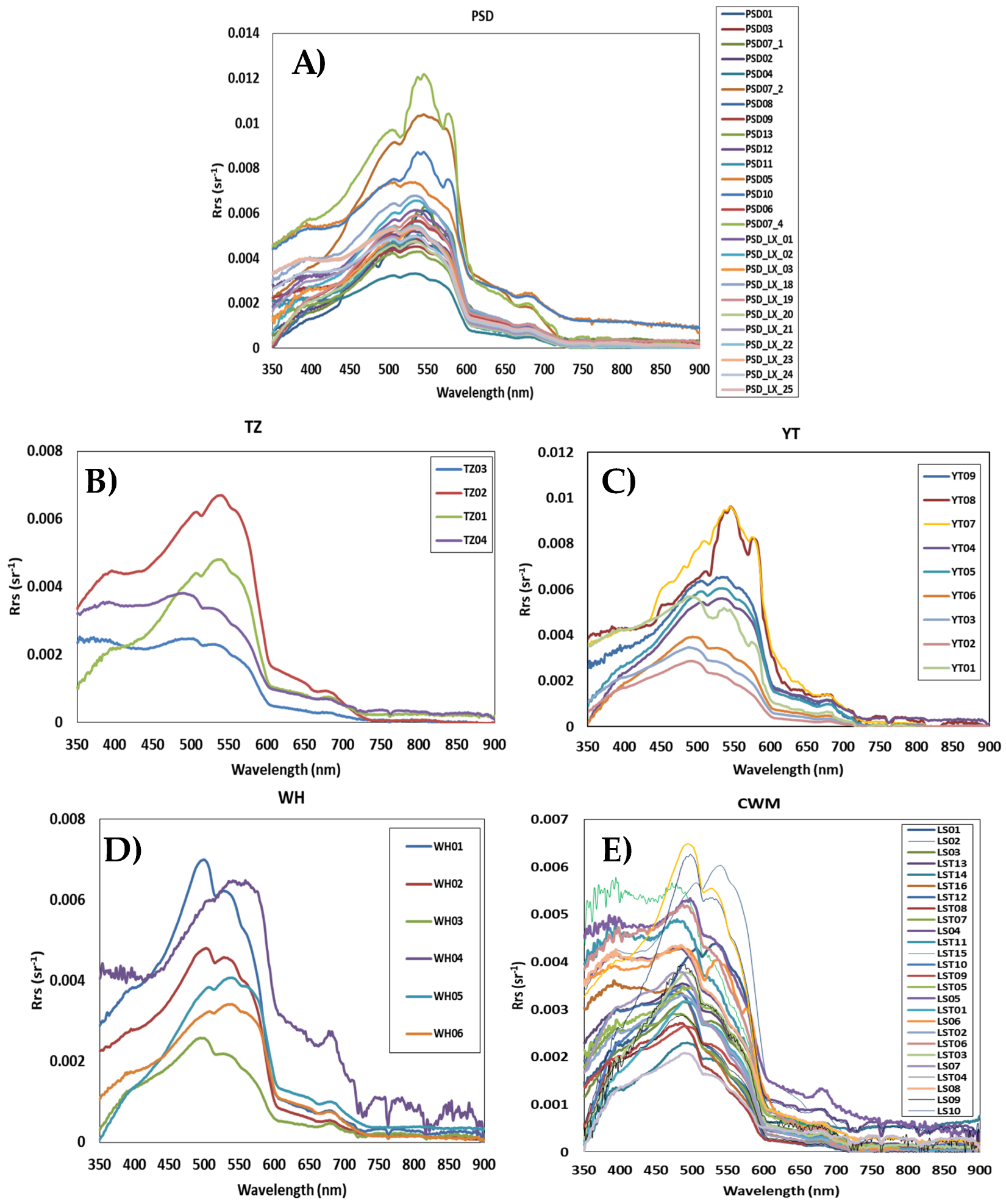
3.2.1. Measurement of Remote Sensing Reflectance
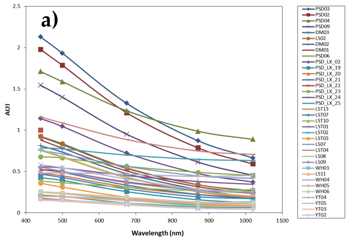
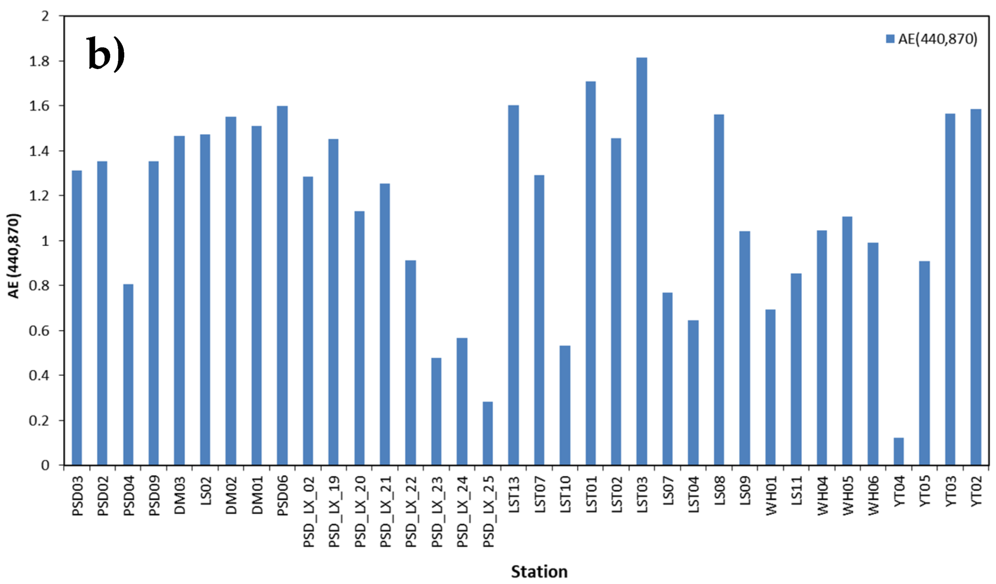
3.2.2. Measurement of Aerosol Optical Properties
3.2.3. Measurement of Chla Data
3.3. GOCI Data
3.4. Match-Ups Procedures
3.5. Statistical Metrics
4. Results
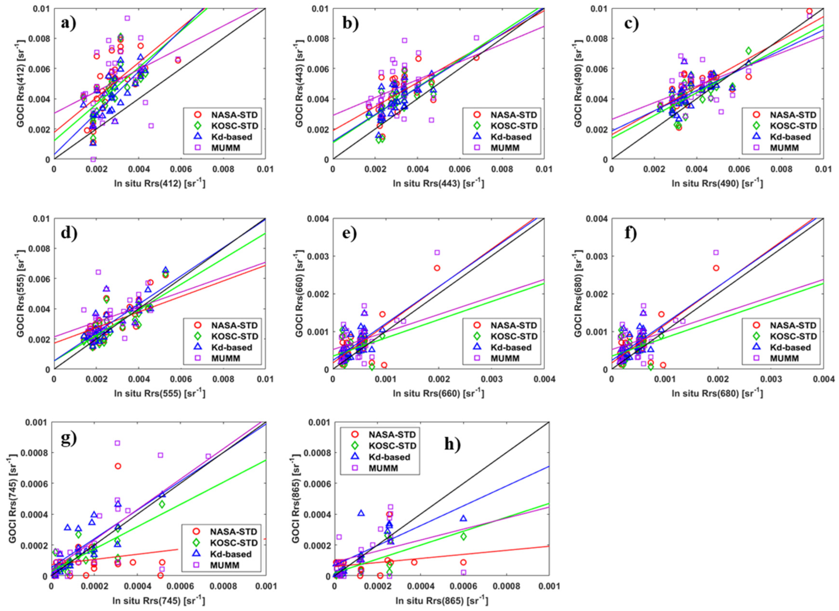
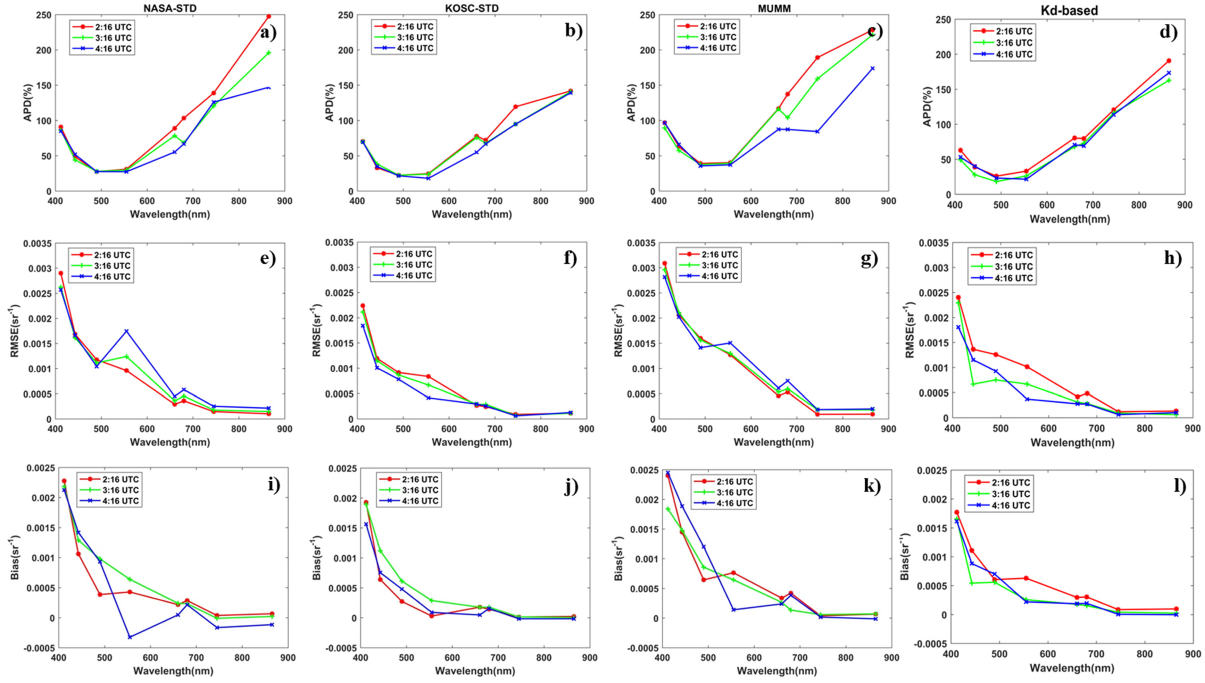
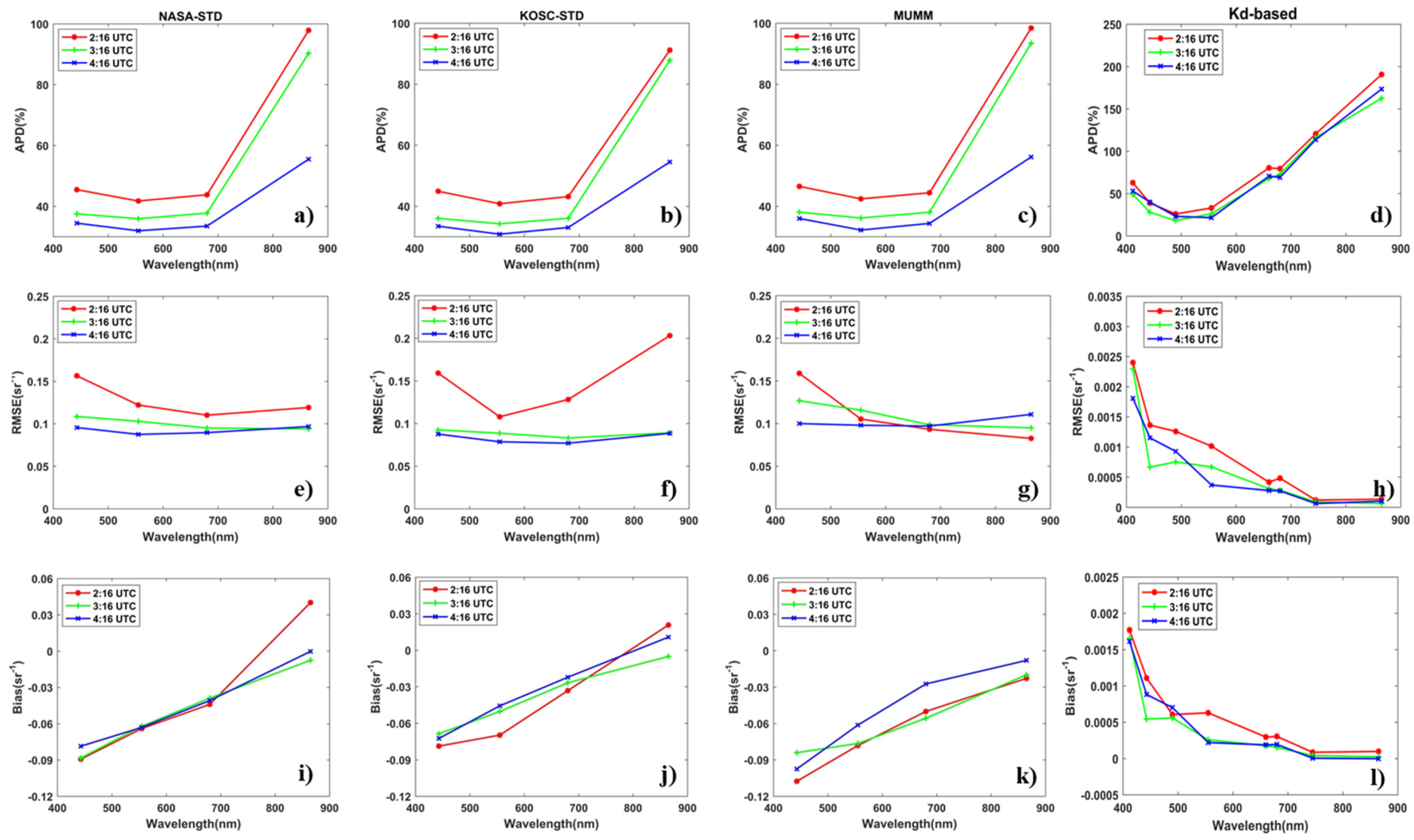
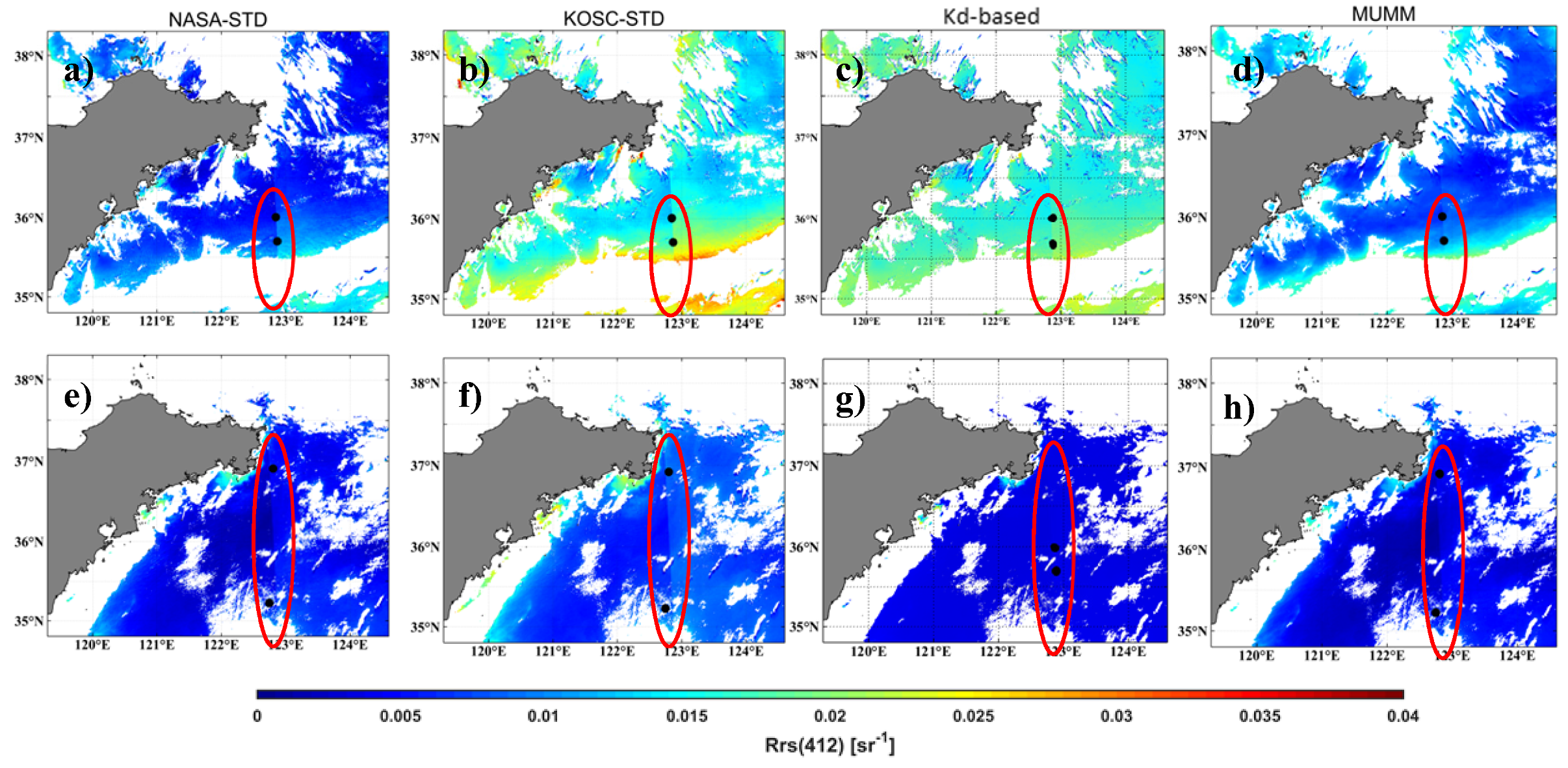
4.1. Comparison of Rrs
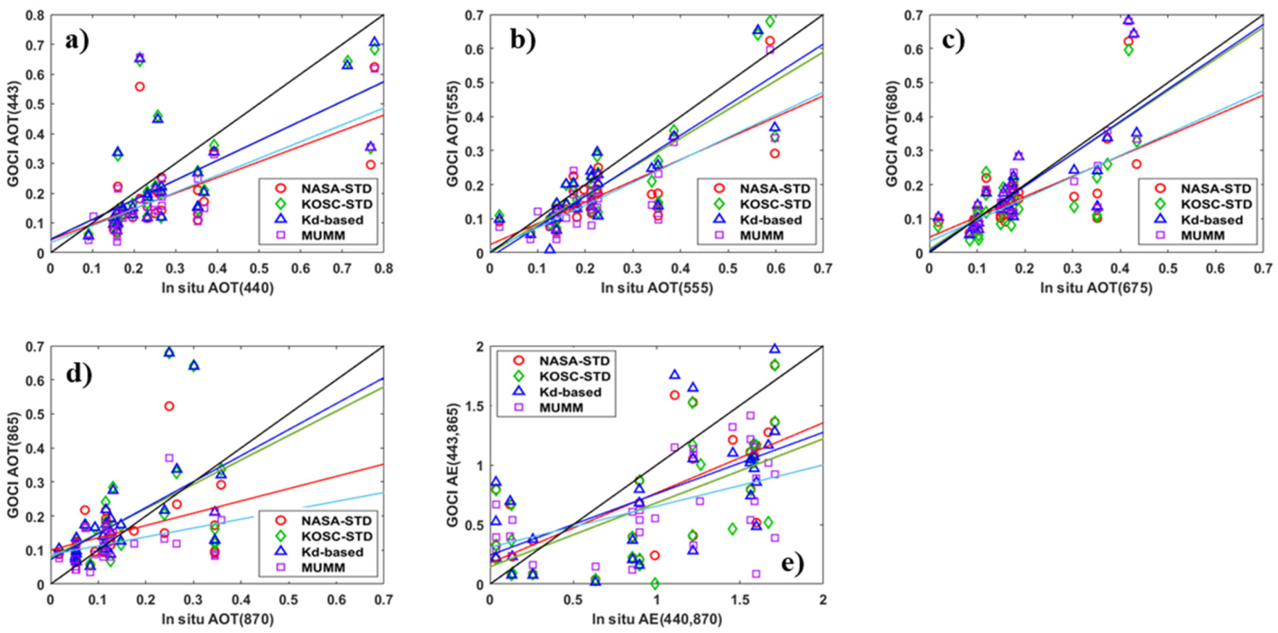
4.2. Comparison of AOT and AE
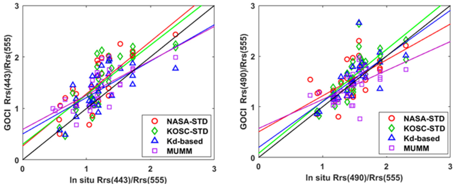
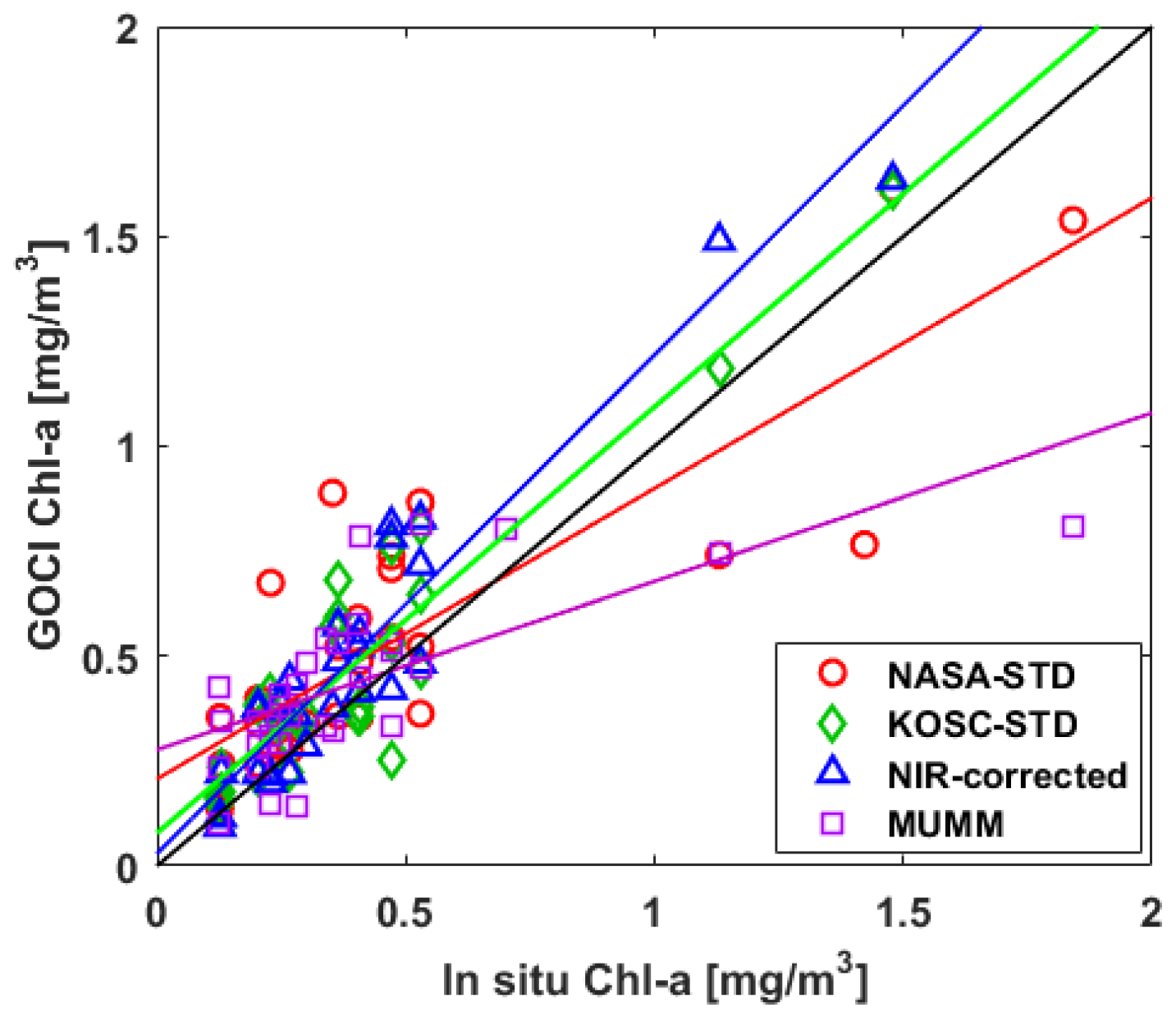
4.3. Comparison of OC3G Chla Retrievals
5. Discussion
6. Conclusions
Author Contributions
Funding
Acknowledgments
Conflicts of Interest
Appendix A

References
- Sathyendranath, S. (Ed.) Remote Sensing of Ocean Colour in Coastal, and Other Optically-Complex, Waters; Reports of the International Ocean-Colour Coordinating Group, No. 3; IOCCG: Dartmouth, NS, Canada, 2000. [Google Scholar]
- Morel, A.; Prieur, L. Analysis of variations in ocean color. Limnol. Oceanogr. 1977, 22, 709–722. [Google Scholar] [CrossRef]
- Kim, W.; Moon, J.; Park, Y.; Ishizaka, J. Evalution of chlorophyll retrievals from Geostationary Ocean color Imager (GOCI) for the North-East Asian region. Remote Sens. Environ. 2016, 184, 482–495. [Google Scholar] [CrossRef]
- Wang, M.H. (Ed.) Atmospheric Correction for Remotely-Sensed Ocean-Colour Products; Reports of the International Ocean-Colour Coordinating Group, No. 10; IOCCG: Darmouth, NS, Canada, 2010; p. 78. [Google Scholar]
- Franz, B.A.; Bailey, S.W.; Werdell, P.J.; McClain, C.R. Sensor-independent approach to the vicarious calibration of satellite ocean color radiometry. Appl. Opt. 2007, 46, 5068–5082. [Google Scholar] [CrossRef] [PubMed]
- Gordon, H.R.; Wang, M. Retrieval of water-leaving radiance and aerosol optical thickness over the oceans with SeaWiFS: A preliminary algorithm. Appl. Opt. 1994, 33, 443–452. [Google Scholar] [CrossRef]
- Siegel, D.A.; Wang, M.; Maritonera, S.; Robinson, W. Atmospheric correction of satellite ocean color imagery: The black pixel assumption. Appl. Opt. 2000, 39, 3582–3591. [Google Scholar] [CrossRef] [PubMed]
- Wang, M.; Knobelspiesse, K.D.; McClain, C.R. Study of the Sea-Viewing Wide Field-of-View Sensor (SeaWiFS) aerosol optical property data over ocean in combination with the ocean color products. J. Geophys. Res. 2005, 110, D10S06. [Google Scholar] [CrossRef]
- Jamet, C.; Loisel, H.; Kuchinke, C.P. Comparison of three SeaWiFS atmospheric correction algorithms for turbid waters using AERONET-OC measurements. Remote Sens. Environ. 2011, 115, 1955–1965. [Google Scholar] [CrossRef]
- Goyens, C.; Jamet, C.; Schroeder, T. Evaluation of four atmospheric correction algorithms for MODIS-Aqua images over contrasted coastal waters. Remote Sens. Environ. 2013, 131, 63–75. [Google Scholar] [CrossRef]
- Hu, C.; Carder, K.L.; Muller-Karger, F.E. Atmospheric correction of SeaWiFS imagery over turbid coastal waters: A practical method. Remote Sens. Environ. 2000, 74, 195–206. [Google Scholar] [CrossRef]
- Ruddick, K.; Ovidio, F.; Rijkeboer, M. Atmospheric correction of SeaWiFS imagery for turbid coastal and inland waters. Appl. Opt. 2000, 39, 897–912. [Google Scholar] [CrossRef]
- Wang, M.; Shi, W.; Jiang, L. Atmospheric correction using near-infrared bands for satellite ocean color data processing in the turbid western Pacific region. Opt. Express 2012, 20, 741–753. [Google Scholar] [CrossRef] [PubMed]
- Dogliotti, A.I.; Ruddick, K.; Nechad, B.; Lasta, C. Improving water reflectance retrieval from MODIS imagery in the highly turbid waters of La Plata River. In Proceedings of the VI International Conference “Current Problems in Optics of Natural Waters”, St. Petersburg, Russia, 6–9 September 2011; pp. 1–8. [Google Scholar]
- Wang, M.; Shi, W. The NIR-SWIR combined atmospheric correction approach for MODIS ocean color data processing. Opt. Express 2007, 15, 15722–15733. [Google Scholar] [CrossRef]
- Wang, M.; Son, S.; Shi, W. Evaluation of MODIS SWIR and NIR-SWIR atmospheric correction algorithms using SeaBASS data. Remote Sens. Environ. 2009, 113, 635–644. [Google Scholar] [CrossRef]
- Oo, M.; Vargas, M.; Gilerson, A.; Gross, B.; Moshary, F.; Ahmed, S. Improving atmospheric correction for highly productive coastal waters using the short wave infrared retrieval algorithm with water-leaving reflectance constraints at 412 nm. Appl. Opt. 2008, 47, 3846–3859. [Google Scholar] [CrossRef] [PubMed]
- He, X.; Bai, Y.; Pan, D. Atmospheric correction of satellite ocean color imagery using the ultraviolet wavelength for highly turbid waters. Opt. Express 2012, 20, 20754–20770. [Google Scholar] [CrossRef] [PubMed]
- Stumpf, R.P.; Arnone, R.A.; Gould, R.W. A Partially Coupled Ocean-Atmosphere Model for Retrieval of Water-Leaving Radiance from SeaWiFS in Coastal Waters. SeaWiFS Postlaunch Tech. Rep. Ser. 2003, 206892, 51–59. [Google Scholar]
- Lavender, S.J.; Pinkerton, M.H.; Moore, G.F.; Aiken, J.; Blondeau-Patissier, D. Modification to the atmospheric correction of SeaWiFS ocean colour images over turbid waters. Cont. Shelf Res. 2005, 25, 539–555. [Google Scholar] [CrossRef]
- Jamet, C.; Thiria, S.; Moulin, C. Use of a Neurovariational Inversion for Retrieving Oceanic and Atmospheric Constituents from Ocean Color Imagery: A Feasibility Study. J. Atmos. Ocean. Tech. 2005, 22, 460–475. [Google Scholar] [CrossRef]
- Schroeder, T.; Behnert, I.; Schaale, M.; Fischer, J.; Doerffer, R. Atmospheric correction algorithm for MERIS above case-2 waters. J. Remote Sens. 2007, 28, 1469–1486. [Google Scholar] [CrossRef]
- Jamet, C.; Thiria, S.; Moulin, C.; Crepon, M. Use of a neuro-variational inversion for retrieving oceanic and atmospheric constituents from satellite ocean color sensor: Application to absorbing aerosols. Neural Netw. 2006, 22, 460–475. [Google Scholar]
- Kuchinke, C.P.; Gordon, H.R.; Harding, L.W.; Voss, K.J., Jr. Spectral optimization for constituent retrieval in Case II waters II: Validation study in the Chesapeake Bay. Remote Sens. Environ. 2009, 113, 610–621. [Google Scholar] [CrossRef]
- Steinmetz, F.; Ramon, D.; Deschamps, I.; Stum, J. Improved Global Ocean Color Using Polymer Algorithm. In Proceedings of the ESA Living Planet Symposium, Bergen, Norway, 28 June–2 July 2010. [Google Scholar]
- Zibordi, G.; Melin, F.; Berthon, J.F. Comparison of SeaWiFS, MODIS and MERIS radiometric products at a coastal site. Geophys. Res. Lett. 2006, 33, L06617. [Google Scholar] [CrossRef]
- Ahn, J.Y.; Ryu, J.Y.; Park, Y.J.; Ahn, Y.J.; Oh, I.S. Atmospheric Correction Algorithm for the GOCI; IGARSS: Munich, Germany, 2012. [Google Scholar]
- Bailey, S.W.; Franz, B.A.; Werdell, P.J. Estimation of near-infraredwater-leaving reflectance for satellite ocean color data processing. Opt. Express 2010, 18, 7521–7527. [Google Scholar] [CrossRef] [PubMed]
- Ahn, J.Y.; Park, Y.J.; Ryu, J.H. Development of atmospheric correction algorithm for Geostationary Ocean Color Imager (GOCI). Ocean Sci. J. 2012, 47, 247–259. [Google Scholar] [CrossRef]
- Shi, W.; Wang, M. Satellite views of the Bohai Sea, Yellow Sea, and East China Sea. Prog. Oceanogr. 2012, 104, 30–45. [Google Scholar] [CrossRef]
- Gordon, H.R.; Wang, M. Surface-roughness considerations for atmospheric correction of ocean color sensors I: The Rayleigh-scattering component. Appl. Opt. 1992, 31, 4247–4260. [Google Scholar] [CrossRef] [PubMed]
- Zhang, H.; Wang, M. Evaluation of sun glint models using MODIS measurements. J. Quant. Spectrosc. Radiat. Transf. 2010, 111, 492–506. [Google Scholar] [CrossRef]
- Frouin, R.; Schwindling, M.; Dechamps, P.Y. Spectral reflectance of sea foam in the visible and near infrared:In situ measurements and remote sensing implications. J. Geophys. Res. 1996, 101, 14361–14371. [Google Scholar] [CrossRef]
- Ahmad, Z.; Franz, B.A.; McClain, C.R.; Kwiatkowska, E.J.; Werdell, J.; Shettle, E.P.; Holben, B.N. New aerosol models for the retrieval of aerosol optical thickness and normalized water-leaving radiances from the SeaWiFS and MODIS sensors over coastal regions and open oceans. Appl. Opt. 2010, 49, 5545–5560. [Google Scholar] [CrossRef] [PubMed]
- O’Reilly, J.; Maritorena, S.; Siegel, D. SeaWiFS Postlaunch Calibration and Validation Analyses, Part 3. In NASA Technical Memorandum; Hooker, S., Firestone, E., Eds.; NASA Goddard Space Flight Center: Greenbelt, MD, USA, 2000; p. 33. [Google Scholar]
- Lee, Z.; Carder, K.L.; Arnone, R.A. Deriving inherent optical properties from water color: A multiband quasi-analytical algorithm for optically deep waters. Appl. Opt. 2002, 41, 5755–5772. [Google Scholar] [CrossRef]
- Ahn, Y.; Han, H.; Yang, H.; Moon, J.; Ahn, J.; Lee, B.; Min, J.; Lee, S.; Kim, K.; Han, T.; et al. GDPS ATBD (Ver.1.3): GOCI Level 2 Ocean Color Products (GDPS 1.3) Brief Algorithm Description. Available online: http://kosc.kiost.ac.kr/eng/p30/kosc_p34.html (accessed on 17 November 2014).
- Wang, M.; Ahn, J.H.; Jiang, L. Ocean color products from the Korean Geostationary Ocean Color Imager (GOCI). Opt. Express 2013, 21, 3835. [Google Scholar] [CrossRef] [PubMed]
- Ruddick, K.G.; De Cauwer, V.; Park, Y.-J.; Mooe, G. Seaborne measurements of near infrared water-leaving reflectance: The similarity spectrum for turbid waters. Limnol. Oceanogr. 2006, 51, 1167–1179. [Google Scholar] [CrossRef]
- Gohin, F.; Druon, J.N.; Lampert, L. A five channel chlorophyll concentration algorithm applied to SeaWiFS data processed by SeaDAS in coastal waters. Int. J. Remote Sens. 2002, 23, 1639–1661. [Google Scholar] [CrossRef]
- Komick, N.M.; Costa, M.P.F.; Gower, J. Bio-opticalalgorithm evaluation for MODIS for western Canada coastal waters: An exploratory approach using in situ reflectance. Remote Sens. Environ. 2009, 113, 794–804. [Google Scholar] [CrossRef]
- Hu, C.; Feng, L.; Lee, Z.P. Evaluation of GOCI sensitivity for At-Sensor radiance and GDPS-Retrieved chlorophyll-aproducts. Ocean Sci. J. 2012, 47, 279–285. [Google Scholar] [CrossRef]
- Minu, P.; Lotliker, A.A.; Shaju, S.S.; Ashraf, P.M.; Kumar, T.S.; Meenakumari, B. Performance of operational satellite bio-optical algorithms in different water types in the southeastern Arabian Sea. Oceanologia 2016, 58, 317–326. [Google Scholar] [CrossRef]
- Cui, T.; Zhang, J.; Tang, J. Assessment of satellite ocean color products of MERIS, MODIS and SeaWiFS along the East China Coast (in the Yellow Sea and East China Sea). ISPRS J. Photogramm. Remote Sens. 2014, 87, 137–151. [Google Scholar] [CrossRef]
- Shi, W.; Wang, M. Green macroalgae blooms in the Yellow Sea during the spring and summer of 2008. J. Geophys. Res. 2009, 114, C12010. [Google Scholar] [CrossRef]
- Gong, G.; Wen, Y.; Wang, B.; Liu, G. Seasonal variation of chlorophyll a concentration, primary production and environmental conditions in the subtropical East China Sea. Deep Sea Res. II 2003, 50, 1219–1236. [Google Scholar] [CrossRef]
- Siswanto, E.; Ishizaka, J.; Yokouchi, K. Optimal primary production model and parameterization in the eastern East China Sea. J. Oceanogr. 2006, 62, 361–372. [Google Scholar] [CrossRef]
- Li, H.; Tian, X.; Tao, D. Effect of the Yellow Sea Cold Water Mass (YSCWM) on distribution of bacterioplankton. Acta Ecol. Sin. 2006, 26, 1012–1019. [Google Scholar] [CrossRef]
- Son, S.H.; Wang, M. The Diffuse Attenuation Coefficient Model in the Yellow Sea for the Korean Geostationary Ocean Color Imager (GOCI). In Proceedings of SPIE; The International Society for Optical Engineering: Bellingham, WA, USA, 2010; Volume 7861. [Google Scholar]
- Mueller, J.; Pietras, C.; Hooker, S.; Clark, D.; Morel, A.; Frouin, R.; Mitchell, B.; Bidigare, R.; Trees, C.; Werdell, J.; et al. Ocean Optics Protocols For Satellite Ocean Color Sensor Validation, Revision 3; Mueller, J.L., Fargion, G.S., Eds.; Goddard Space Flight Space Center: Greenbelt, MD, USA, 2002.
- Mobley, C.D. Estimation of the remote-sensing reflectance from above-surface measurements. Appl. Opt. 1999, 38, 7442–7455. [Google Scholar] [CrossRef] [PubMed]
- Mobley, C.D. Polarized reflectance and transmittance properities of windblown sea surfaces. Appl. Opt. 2015, 54, 4828–4849. [Google Scholar] [CrossRef] [PubMed]
- Cui, T.W.; Song, Q.J.; Tang, J.W. Spectral variability of sea surface skylight reflectance and its effect on ocean color. Opt. Express 2013, 21, 24929. [Google Scholar] [CrossRef]
- Lee, Z.P.; Ahn, Y.H.; Mobley, C. Removal of surface-reflected light for the measurement of remote-sensing reflectance from an above-surface platform. Opt. Express 2010, 18, 26313–26324. [Google Scholar] [CrossRef]
- Holben, B.N.; Eck, T.F.; Slutker, I.; Tanré, D.; Buis, J.P.; Setzer, A.; Vermote, E.; Reagan, J.A.; Kaufman, Y.J.; Nakajima, T.; et al. AERONET—A federated instrument network and data archive for aerosol characterization. Remote Sens. Environ. 1998, 66, 1–16. [Google Scholar] [CrossRef]
- Smirnov, A.; Holben, B.N.; Eck, T.F.; Dubovik, O.; Slutsker, I. Cloud-screening and quality control algorithms for the AERONET database. Remote Sens. Environ. 2000, 73, 337–349. [Google Scholar] [CrossRef]
- Mueller, J.L.; Bidigare, R.R.; Trees, C.; Balch, W.M.; Dore, J.; Drapeau, D.T.; Karl, D.; Van Heukelem, L.; Perl, J. Ocean Optics Protocols for Satellite Ocean Color Sensor Validation, Revision 5: Biogeochemical and Bio- Optical Measurements and Data Analysis Protocols; Mueller, J.L., Fargion, G.S., McClain, C.R., Eds.; NASA Goddard Space Flight Center: Greenbelt, MD, USA, 2003; Volume 5, pp. 1–43. Available online: https://seabass.gsfc.nasa.gov/wiki/System_Description/Protocols_Ver5_VolV.pdf (accessed on 19 October 2017).
- Ryu, J.H.; Han, H.J.; Cho, S. Overview of geostationary ocean color imager (GOCI) and GOCI data processing system (GDPS). Ocean Sci. J. 2012, 47, 223–233. [Google Scholar] [CrossRef]
- Bailey, S.W.; Werdell, P.J. A multi-sensor approach for the on-orbit validation of ocean color satellite data products. Remote Sens. Environ. 2006, 102, 12–23. [Google Scholar] [CrossRef]
- Lamquin, N.; Mazeran, C.; Doxaran, D. Assessment of GOCI radiometric products using MERIS, MODIS and field measurements. Ocean Sci. J. 2012, 47, 287–311. [Google Scholar] [CrossRef]
- Carswell, T.; Costa, M.; Young, E. Evaluation of MODIS-Aqua Atmospheric Correction and Chlorophyll Products of Western North American Coastal Waters Based on 13 Years of Data. J. Remote Sens. 2017, 9, 1063. [Google Scholar] [CrossRef]
- Eck, T.F.; Holben, B.N.; Reid, J.S.; Dubovik, O.; Smirnov, A.; O’Neill, N.T. The wavelength dependence of the optical depth of biomass burning, urban and desert dust aerosols. J. Geophys. Res. 1999, 104, 31333–31350. [Google Scholar] [CrossRef]
- Schuster, G.L.; Dubovik, O.; Holben, B.N. Angstrom exponent and bimodal size distributions. J. Geophys. Res. Atmos. 2006, 111, 1–14. [Google Scholar] [CrossRef]
- Choi, J.K.; Park, Y.J.; Ahn, J.H. GOCI, the world’s first geostationary ocean color observation satellite, for the monitoring of temporal variability in coastal water turbidity. J. Geophys. Res. Oceans 2012, 117. [Google Scholar] [CrossRef]
- Goyens, C.; Jamet, C.; Ruddick, K.G. Spectral relationships for atmospheric correction I Validation of red and near infra-red marine reflectance relationships. Opt. Express 2013, 21, 21162. [Google Scholar] [CrossRef] [PubMed]
- Luo, Y.; Doxaran, D.; Ruddick, K.; Shen, F.; Gentili, B.; Yan, L.; Huang, H. Saturation of water reflectance in extremely turbid media based on field measurements, satellite data and bio-optical modelling. Opt. Express 2018, 26, 10435. [Google Scholar] [CrossRef] [PubMed]
- Doron, M.; Bélanger, S.; Doxaran, D.; Babin, M. Spectral variations in the near-infrared ocean reflectance. Remote Sens. Environ. 2011, 115, 1617–1631. [Google Scholar] [CrossRef]
- He, X.; Bai, Y.; Wei, J.; Ding, J.; Shanmugam, P.; Wang, D.; Song, Q.; Huang, X. Ocean color retrieval from MWI onboard the Tiangong-2 Space Lab: Preliminary results. Opt. Express 2017, 25, 23955–23973. [Google Scholar] [CrossRef]
- Shettle, E.P.; Fenn, R.W. Models for the Aerosols of the Lower Atmosphere and the Effects of Humidity Variations on Their Optical Properties; No. AFGL-TR-79–0214; Air Force Geophysics Lab: Hanscom AFB, MA, USA, 1979. [Google Scholar]
- Lee, B.; Ahn, J.H.; Kim, W.; Lee, B. Simple aerosol correction technique based on the spectral relationships of the aerosol multiple-scattering reflectances for atmospheric correction over the oceans. Opt. Express 2016, 24, 29659. [Google Scholar]
- Kim, W.; Ahn, J.; Park, Y. Correction of Stray-light Driven Interslot Radiometric Discrepancy (ISRD) Present in Radiometric Products of Geostationary Ocean Color Imager (GOCI). IEEE Trans Geosci. Remote Sens. 2015, 53, 5458–5472. [Google Scholar]
- Concha, J.; Mannino, A.; Franz, B.; Bailey, S.; Kim, W. Vicarious calibration of GOCI for the SeaDAS ocean color retrieval. Int. J. Remote Sens. 2019, 40, 1–18. [Google Scholar] [CrossRef]
- Ahn, J.H.; Park, Y.J.; Kim, W.; Lee, B.; Oh, I.S. Vicarious calibration of the Geostationary Ocean Color Imager. Opt. Express 2015, 23, 23236–23258. [Google Scholar] [CrossRef] [PubMed]
- Amin, R.; Lewis, M.D.; Lawson, A. Comparative Analysis of GOCI Ocean Color Products. Sensors 2015, 15, 25703–25715. [Google Scholar] [CrossRef] [PubMed]
- Lubac, B.; Loisel, H. Variability and classification of remote sensing reflectance spectra in the eastern English Channel and southern North Sea. Remote Sens. Environ. 2007, 110, 45–58. [Google Scholar] [CrossRef]
- Vantrepotte, V.; Loisel, H.; Dessailly, D.; Mériaux, X. Optical classification of contrasted coastal waters. Remote Sens. Environ. 2012, 123, 306–323. [Google Scholar] [CrossRef]
- Mobley, C.D.; Werdell, P.J.; Franz, B. Atmospheric Correction for Satellite Ocean Color Radiometry: A Tutorial and Documentation of the Algorithms Used by the NASA Ocean Biology Processing Group; Sequoia Scientific, Inc.: Bellevue, WA, USA, 2016. [Google Scholar]
- Torres, O.; Bhartia, P.K.; Herman, J.R. Derivation of aerosol properties from satellite measurements of backscattered ultraviolet radiation: Theoretical basis. J. Geophys. Res. 1998, 103, 23321–23322. [Google Scholar] [CrossRef]
- Cho, S. Lunar Calibration Workshop, Introduction of GOCI and GOCI-II Mission with Lunar Calibration. EUMETSAT, Darmstadt, Germany. Available online: http://gsics.atmos.umd.edu/pub/Development/ LunarCalibrationWorkshop/4b_Cho_GOCI2.pdf (accessed on 12 December 2014).


| Method | Rrs(λ) | %Negative | Count (N) | APD(%) | RMSE(sr−1) | Bias(sr−1) | R2 | Slope | Intercept |
|---|---|---|---|---|---|---|---|---|---|
| NASA-STD | Rrs(412) | 11 (25) | 27 (8) | 94.55 (63.73) | 0.003 (0.002) | 0.002 (0.002) | 0.37 (0.52) | 0.27 (0.36) | 1 × 10⁻³ (1 × 10⁻³) |
| Rrs(443) | 7 (12) | 28 (8) | 47.94 (38.21) | 0.002 (0.001) | 0.001 (0.001) | 0.39 (0.38) | 0.49 (0.49) | 1 × 10⁻³ (1 × 10⁻³) | |
| Rrs(490) | 0 (0) | 30 (10) | 27.58 (20.93) | 0.001 (9 × 10⁻⁴) | 8 × 10⁻⁴ (6 × 10⁻⁴) | 0.67 (0.57) | 0.85 (0.99) | −6 × 10⁻⁵ (−6 × 10⁻⁴) | |
| Rrs(555) | 0 (0) | 30 (10) | 29.25 (16.64) | 0.001 (6 × 10⁻⁴) | 2 × 10⁻⁴ (2 × 10⁻⁴) | 0.60 (0.85) | 1.16 (0.79) | −8 × 10⁻⁴ (5 × 10⁻⁴) | |
| Rrs(660) | 0 (0) | 29 (9) | 74.06 (71.18) | 4 × 10⁻⁴ (3 × 10⁻⁴) | 2 × 10⁻⁴ (2 × 10⁻⁴) | 0.56 (0.31) | 0.55 (0.36) | 1 × 10⁻⁴ (2 × 10⁻⁴) | |
| Rrs(680) | 0 (0) | 28 (8) | 79.42 (89.46) | 5 × 10⁻⁴ (4 × 10⁻⁴) | 2 × 10⁻⁴ (3 × 10⁻⁴) | 0.58 (0.12) | 0.48 (0.28) | 1 × 10⁻⁴ (3 × 10⁻⁴) | |
| Rrs(745) | 6 (11) | 29 (9) | 128.39 (149.75) | 2 × 10⁻⁴ (2 × 10⁻⁴) | −4 × 10⁻⁵ (1 × 10⁻⁵) | 0.03 (0.49) | 0.19 (0.31) | 2 × 10⁻⁴ (9 × 10⁻⁵) | |
| Rrs(865) | 6 (11) | 29 (9) | 196.78 (206.72) | 2 × 10⁻⁴ (9 × 10⁻⁵) | −1 × 10⁻⁵ (4 × 10⁻⁷) | 0.06 (0.29) | 0.44 (0.41) | 1 × 10⁻⁴ (7 × 10⁻⁵) |
| Method | Rrs(λ) | %Negative | Count (N) | APD(%) | RMSE(sr−1) | Bias(sr−1) | R2 | Slope | Intercept |
|---|---|---|---|---|---|---|---|---|---|
| KOSC-STD | Rrs(412) | 3 (11) | 28 (9) | 73.95 (57.00) | 0.002 (2 × 10⁻³) | 0.002 (1 × 10⁻³) | 0.43 (0.64) | 0.38 (0.42) | 1 × 10⁻³ (1 × 10⁻³) |
| Rrs(443) | 3 (11) | 28 (9) | 35.27 (27.33) | 0.001 (8 × 10⁻⁴) | 0.001 (6 × 10⁻⁴) | 0.41 (0.60) | 0.45 (0.57) | 1 × 10⁻³ (1 × 10⁻³) | |
| Rrs(490) | 0 (0) | 29 (10) | 22.08 (17.16) | 9 × 10⁻⁴ (7 × 10⁻⁴) | 5 × 10⁻⁴ (4 × 10⁻⁴) | 0.49 (0.75) | 0.66 (0.74) | 1 × 10⁻³ (8 × 10⁻⁴) | |
| Rrs(555) | 0 (0) | 29 (10) | 22.23 (12.37) | 7 × 10⁻⁴ (4 × 10⁻⁴) | 1 × 10⁻⁴ (1 × 10⁻⁵) | 0.66 (0.90) | 0.78 (0.78) | 5 × 10⁻⁴ (7 × 10⁻⁴) | |
| Rrs(660) | 0 (0) | 28 (10) | 69.79 (61.63) | 3 × 10⁻⁴ (3 × 10⁻⁴) | 1 × 10⁻⁴ (9 × 10⁻⁵) | 0.14 (0.08) | 0.30 (0.27) | 2 × 10⁻⁴ (3 × 10⁻⁴) | |
| Rrs(680) | 0 (0) | 28 (10) | 68.92 (100.53) | 3 × 10⁻⁴ (4 × 10⁻⁴) | 2 × 10⁻⁴ (2 × 10⁻⁴) | 0.23 (5 × 10⁻³) | 0.39 (0.11) | 2 × 10⁻⁴ (4 × 10⁻⁴) | |
| Rrs(745) | 0 (0) | 29 (10) | 103.27 (95.65) | 1 × 10⁻⁴ (7 × 10⁻⁵) | 4 × 10⁻⁶ (−3 × 10⁻⁵) | 0.72 (0.66) | 0.99 (0.87) | 1 × 10⁻⁵ (7 × 10⁻⁵) | |
| Rrs(865) | 0 (0) | 29 (10) | 140.56 (125.78) | 1 × 10⁻⁴ (7 × 10⁻⁵) | 4 × 10⁻⁶ (−2 × 10⁻⁶) | 0.60 (0.53) | 1.34 (0.84) | 2 × 10⁻⁵ (4 × 10⁻⁵) |
| Method | Rrs(λ) | %Negative | Count (N) | APD(%) | RMSE(sr−1) | Bias(sr−1) | R2 | Slope | Intercept |
|---|---|---|---|---|---|---|---|---|---|
| Kd-based | Rrs(412) | 7 (11) | 29 (9) | 53.64 (56.80) | 0.002 (0.002) | 0.001 (0.001) | 0.56 (0.60) | 0.41 (0.32) | 1 × 10⁻³ (0.001) |
| Rrs(443) | 7 (11) | 29 (9) | 32.07 (28.61) | 0.001 (0.001) | 8 × 10⁻⁴ (8 × 10⁻⁴) | 0.45 (0.66) | 0.51 (0.52) | 1 × 10⁻³ (0.001) | |
| Rrs(490) | 0 (0) | 31 (10) | 22.31 (17.44) | 0.001 (8 × 10⁻⁴) | 6 × 10⁻⁴ (6 × 10⁻⁴) | 0.42 (0.63) | 0.69 (0.86) | 6 × 10⁻⁴ (8 × 10⁻⁵) | |
| Rrs(555) | 0 (0) | 31 (10) | 23.68 (14.63) | 8 × 10⁻⁴ (6 × 10⁻⁴) | 4 × 10⁻⁴ (3 × 10⁻⁴) | 0.65 (0.91) | 0.36 (0.77) | 2 × 10⁻⁴ (5 × 10⁻⁴) | |
| Rrs(660) | 0 (0) | 31 (10) | 72.72 (71.12) | 3 × 10⁻⁴ (4 × 10⁻⁴) | 2 × 10⁻⁴ (2 × 10⁻⁴) | 0.35 (0.28) | 0.34 (0.34) | 2 × 10⁻⁴ (2 × 10⁻⁴) | |
| Rrs(680) | 0 (0) | 31 (10) | 72.76 (85.49) | 4 × 10⁻⁴ (5 × 10⁻⁴) | 2 × 10⁻⁴ (3 × 10⁻⁴) | 0.34 (0.39) | 0.34 (0.36) | 2 × 10⁻⁴ (2 × 10⁻⁴) | |
| Rrs(745) | 3 (11) | 30 (9) | 117.97 (62.91) | 9 × 10⁻⁵ (7 × 10⁻⁵) | 5 × 10⁻⁵ (4 × 10⁻⁵) | 0.67 (0.75) | 0.67 (0.63) | 2 × 10⁻⁵ (2 × 10⁻⁵) | |
| Rrs(865) | 3 (11) | 30 (9) | 170.03 (138.48) | 1 × 10⁻⁴ (6 × 10⁻⁵) | 4 × 10⁻⁵ (3 × 10⁻⁵) | 0.64 (0.81) | 0.84 (0.88) | 1 × 10⁻⁵ (2 × 10⁻⁵) |
| Method | Rrs(λ) | %Negative | Count (N) | APD(%) | RMSE(sr−1) | Bias(sr−1) | R2 | Slope | Intercept |
|---|---|---|---|---|---|---|---|---|---|
| MUMM | Rrs(412) | 13 (20) | 31 (10) | 107.47 (74.20) | 0.003 (0.002) | 0.002 (0.002) | 0.10 (0.44) | 0.14 (0.23) | 2 × 10⁻³ (0.002) |
| Rrs(443) | 6 (20) | 31 (10) | 60.41 (46.03) | 0.002 (0.002) | 0.002 (0.001) | 0.28 (0.24) | 0.33 (0.32) | 2 × 10⁻³ (2 × 10⁻³) | |
| Rrs(490) | 0 (0) | 32 (11) | 30.87 (27.14) | 0.001 (0.001) | 7 × 10⁻⁴ (7 × 10⁻⁴) | 0.32 (0.36) | 0.59 (0.73) | 1 × 10⁻³ (6 × 10⁻⁴) | |
| Rrs(555) | 0 (0) | 32 (11) | 38.33 (24.18) | 0.001 (9 × 10⁻⁴) | 5 × 10⁻⁴ (6 × 10⁻⁴) | 0.46 (0.80) | 0.93 (0.73) | −4 × 10⁻⁴ (4 × 10⁻⁴) | |
| Rrs(660) | 0 (0) | 31 (11) | 97.20 (93.42) | 0.001 (5 × 10⁻⁴) | 3 × 10⁻⁴ (3 × 10⁻⁴) | 0.71 (0.30) | 1.53 (0.22) | −6 × 10⁻⁴ (3 × 10⁻⁴) | |
| Rrs(680) | 0 (0) | 32 (10) | 101.78 (125.82) | 6 × 10⁻⁴ (6 × 10⁻⁴) | 3 × 10⁻⁴ (4 × 10⁻⁴) | 0.76 (0.22) | 0.69 (0.22) | −2 × 10⁻⁴ (3 × 10⁻⁴) | |
| Rrs(745) | 6 (18) | 32 (11) | 142.57 (120.50) | 2 × 10⁻⁴ (2 × 10⁻⁴) | 4 × 10⁻⁵ (8 × 10⁻⁵) | 0.52 (0.35) | 0.51 (0.23) | 8 × 10⁻⁵ (7 × 10⁻⁵) | |
| Rrs(865) | 6 (18) | 32 (11) | 193.32 (244.88) | 1 × 10⁻⁴ (2 × 10⁻⁴) | 3 × 10⁻⁵ (9 × 10⁻⁵) | 0.13 (0.53) | 0.36 (0.30) | 9 × 10⁻⁵ (3 × 10⁻⁵) |
| Method | Band Ratio | APD(%) | RMSE(sr−1) | Bias(sr−1) | R2 | Slope | Intercept |
|---|---|---|---|---|---|---|---|
| NASA-STD | Rrs(443)/Rrs(555) | 34.11 (34.14) | 0.424 (0.414) | 0.287 (0.326) | 0.61 (0.74) | 0.60 (0.59) | 0.29 (0.24) |
| Rrs(490)/Rrs(555) | 18.73 (14.73) | 0.309 (0.252) | 0.089 (0.145) | 0.40 (0.72) | 0.57 (0.65) | 0.57 (0.37) | |
| KOSC-STD | Rrs(443)/Rrs(555) | 27.05 (29.27) | 0.402 (0.428) | 0.257 (0.282) | 0.63 (0.80) | 0.66 (0.50) | 0.26 (0.38) |
| Rrs(490)/Rrs(555) | 14.49 (19.45) | 0.309 (0.414) | 0.119 (0.224) | 0.58 (0.79) | 0.57 (0.45) | 0.59 (0.63) | |
| Kd-based | Rrs(443)/Rrs(555) | 23.01 (19.61) | 0.332 (0.306) | 0.149 (0.160) | 0.46 (0.72) | 0.64 (0.58) | 0.34 (0.35) |
| Rrs(490)/Rrs(555) | 11.43 (14.55) | 0.272 (0.386) | 0.054 (0.139) | 0.49 (0.66) | 0.55 (0.44) | 0.64 (0.69) | |
| MUMM | Rrs(443)/Rrs(555) | 28.19 (26.61) | 0.338 (0.313) | 0.194 (0.190) | 0.54 (0.56) | 0.81 (0.60) | 0.07 (0.33) |
| Rrs(490)/Rrs(555) | 14.92 (16.56) | 0.287 (0.263) | −0.054 (0.012) | 0.32 (0.37) | 0.57 (0.53) | 0.67 (0.65) |
| Method | Parameter | Count (N) | APD(%) | RMSE(sr−1) | Bias(sr−1) | R2 | Slope | Intercept |
|---|---|---|---|---|---|---|---|---|
| NASA-STD | AOT(443) | 27 (8) | 41.29 (38.38) | 0.148 (0.090) | −0.083 (−0.082) | 0.41 (0.70) | 0.78 (1.14) | 0.12 (0.06) |
| AOT(555) | 30 (10) | 40.88 (33.81) | 0.106 (0.083) | −0.063 (−0.067) | 0.57 (0.49) | 0.91 (1.13) | 0.08 (0.05) | |
| AOT(680) | 28 (8) | 42.46 (30.23) | 0.099 (0.069) | −0.031 (−0.038) | 0.37 (0.38) | 0.62 (1.07) | 0.09 (0.03) | |
| AOT(865) | 29 (9) | 78.99 (37.72) | 0.104 (0.066) | 0.011 (−0.003) | 0.17 (0.32) | 0.47 (1.10) | 0.07 (9 × 10⁻³) | |
| AE(443,865) | 27 (8) | 209.81 (138.54) | 0.808 (0.546) | −0.926 (−0.425) | 0.11 (0.61) | 0.30 (1.13) | 0.45 (0.35) |
| Method | Parameter | Count (N) | APD(%) | RMSE(sr−1) | Bias(sr−1) | R2 | Slope | Intercept |
|---|---|---|---|---|---|---|---|---|
| KOSC-STD | AOT(443) | 28 (9) | 40.51 (50.66) | 0.148 (0.161) | −0.051 (0.019) | 0.46 (0.19) | 0.70 (0.17) | 0.12 (0.18) |
| AOT(555) | 29 (10) | 39.83 (22.79) | 0.092 (0.051) | −0.040 (−0.025) | 0.69 (0.65) | 0.82 (0.74) | 0.08 (0.07) | |
| AOT(680) | 28 (10) | 41.25 (25.48) | 0.098 (0.054) | −0.004 (9 × 10⁻⁴) | 0.55 (0.53) | 0.60 (0.74) | 0.08 (0.04) | |
| AOT(865) | 29 (10) | 75.26 (64.42) | 0.135 (0.091) | 0.035 (0.021) | 0.25 (0.08) | 0.35 (0.34) | 0.09 (0.07) | |
| AE(443,865) | 28 (9) | 206.82 (262.02) | 0.760 (0.672) | −0.842 (−0.439) | 0.13 (0.20) | 0.15 (0.62) | 0.08 (0.65) |
| Method | Parameter | Count (N) | APD(%) | RMSE(sr−1) | Bias(sr−1) | R2 | Slope | Intercept |
|---|---|---|---|---|---|---|---|---|
| Kd-based | AOT(443) | 29 (9) | 40.89 (51.82) | 0.148 (0.162) | −0.051 (0.016) | 0.46 (0.17) | 0.70 (0.16) | 0.12 (0.18) |
| AOT(555) | 31 (10) | 41.17 (33.53) | 0.094 (0.066) | −0.039 (−0.030) | 0.70 (0.59) | 0.78 (0.57) | 0.08 (0.10) | |
| AOT(680) | 31 (10) | 42.18 (28.61) | 0.097 (0.056) | −0.005 (−0.005) | 0.57 (0.50) | 0.60 (0.71) | 0.08 (0.05) | |
| AOT(865) | 30 (10) | 71.77 (57.95) | 0.131 (0.079) | 0.036 (0.024) | 0.29 (0.25) | 0.38 (0.58) | 0.08 (0.04) | |
| AE(443,865) | 29 (9) | 202.36 (275.17) | 0.551 (0.616) | −0.231 (−0.262) | 0.09 (0.17) | 0.71 (0.47) | 0.44 (0.66) |
| Method | Parameter | Count (N) | APD(%) | RMSE(sr−1) | Bias(sr−1) | R2 | Slope | Intercept |
|---|---|---|---|---|---|---|---|---|
| MUMM | AOT(443) | 29 (9) | 40.89 (51.82) | 0.148 (0.162) | −0.051 (0.016) | 0.46 (0.17) | 0.70 (0.16) | 0.12 (0.18) |
| AOT(555) | 31 (10) | 41.17 (33.53) | 0.094 (0.066) | −0.039 (−0.030) | 0.70 (0.59) | 0.78 (0.57) | 0.08 (0.10) | |
| AOT(680) | 31 (10) | 42.18 (28.61) | 0.097 (0.056) | −0.005 (−0.005) | 0.57 (0.50) | 0.60 (0.71) | 0.08 (0.05) | |
| AOT(865) | 30 (10) | 71.77 (57.95) | 0.131 (0.079) | 0.036 (0.024) | 0.29 (0.25) | 0.38 (0.58) | 0.08 (0.04) | |
| AE(443,865) | 29 (9) | 202.36 (275.17) | 0.551 (0.616) | −0.231 (−0.262) | 0.09 (0.17) | 0.71 (0.47) | 0.44 (0.66) |
| Method | Parameter | Confidence Interval (mg m−3) | APD(%) | RMSE(sr−1) | Bias(sr−1) | R2 | Slope | Intercept |
|---|---|---|---|---|---|---|---|---|
| NASA-STD | Chla | (0.41,0.66) (0.33,0.84) | 45.43 (39.82) | 0.235 (0.215) | 0.084 (0.068) | 0.71 (0.76) | 0.82 (0.92) | 0.29 (0.21) |
| KOSC-STD | Chla | (0.35,0.58) (0.27,0.86) | 37.56 (30.11) | 0.146 (0.141) | 0.043 (0.010) | 0.85 (0.92) | 0.84 (0.88) | −0.01 (0.01) |
| NIR-corrected | Chla | (0.36,0.63) (0.27,0.94) | 33.47 (22.05) | 0.160 (0.168) | 0.063 (0.054) | 0.83 (0.87) | 0.76 (0.79) | 0.01 (0.04) |
| MUMM | Chla | (0.37,0.50) (0.27,0.52) | 48.73 (31.85) | 0.244 (0.163) | 0.102 (0.092) | 0.46 (0.67) | 0.64 (0.61) | 0.35 (0.34) |
© 2019 by the authors. Licensee MDPI, Basel, Switzerland. This article is an open access article distributed under the terms and conditions of the Creative Commons Attribution (CC BY) license (http://creativecommons.org/licenses/by/4.0/).
Share and Cite
Huang, X.; Zhu, J.; Han, B.; Jamet, C.; Tian, Z.; Zhao, Y.; Li, J.; Li, T. Evaluation of Four Atmospheric Correction Algorithms for GOCI Images over the Yellow Sea. Remote Sens. 2019, 11, 1631. https://doi.org/10.3390/rs11141631
Huang X, Zhu J, Han B, Jamet C, Tian Z, Zhao Y, Li J, Li T. Evaluation of Four Atmospheric Correction Algorithms for GOCI Images over the Yellow Sea. Remote Sensing. 2019; 11(14):1631. https://doi.org/10.3390/rs11141631
Chicago/Turabian StyleHuang, Xiaocan, Jianhua Zhu, Bing Han, Cédric Jamet, Zhen Tian, Yili Zhao, Jun Li, and Tongji Li. 2019. "Evaluation of Four Atmospheric Correction Algorithms for GOCI Images over the Yellow Sea" Remote Sensing 11, no. 14: 1631. https://doi.org/10.3390/rs11141631
APA StyleHuang, X., Zhu, J., Han, B., Jamet, C., Tian, Z., Zhao, Y., Li, J., & Li, T. (2019). Evaluation of Four Atmospheric Correction Algorithms for GOCI Images over the Yellow Sea. Remote Sensing, 11(14), 1631. https://doi.org/10.3390/rs11141631