Abstract
Semantic segmentation is an important process of scene recognition with deep learning frameworks achieving state of the art results, thus gaining much attention from the remote sensing community. In this paper, an end-to-end conditional random fields generative adversarial segmentation network is proposed. Three key factors of this algorithm are as follows. First, the network combines generative adversarial network and Bayesian framework to realize the estimation from the prior probability to the posterior probability. Second, the skip connected encoder-decoder network is combined with CRF layer to implement end-to-end network training. Finally, the adversarial loss and the cross-entropy loss guide the training of the segmentation network through back propagation. The experimental results show that our proposed method outperformed FCN in terms of mIoU for 0.0342 and 0.11 on two data sets, respectively.
1. Introduction
1.1. Background
Scene recognition has important applications in inferring information through images, such as automatic driving, human-computer intersection and virtual reality. Semantic segmentation plays an important role in scene recognition and paves the way for the complete understanding of the scene, receiving more and more research and studies.
Traditional image segmentation methods include edge-based [1], region-based [2,3] and hybrid segmentation. Since the convolutional neural networks (CNNs) have outstanding performance in various kinds of computer vision tasks [4,5,6,7], the ability of CNNs in semantic segmentation has attracted much attention [8,9,10,11,12]. The state-of-art semantic segmentation algorithm converts CNNs designed for classification such as AlexNet [13] and VGG-16 [6] into fully convolutional network (FCN) [14]. FCN completes the transformation from classification model to semantic segmentation model by replacing the fully-connected layers with deconvolution ones. Image segmentation models based on CNNs can be divided into three categories: (1) The encoder-decoder neural network, such as SegNet [15] and U-Net [16]. In the encoding part, the feature map is generated by removing the last fully connection layer of the network. And then in the decoding part, different structures are utilized to decode the feature map to obtain the image with original size. The decoding part of SegNet consists of up-sampling layers and convolutional layers, each up-sampling layer is determined by its corresponding maximum pooling coefficient of the encoding part. And the convolutional layers are used to generate the dense feature map. (2) The atrous convolution pooling neural network, such as Deeplab [17]. Deeplab proposes atrous convolution, atrous spatial pyramid pooling (ASPP) model and the fully connected conditional random field (CRF). ASPP replaces the original preprocessing method of resizing the image, thus, the input image can have arbitrary scale. The fully connected CRF optimizes local features of classification by using low-level detail information. (3) The image pyramid neural network, such as PSPNet [18]. Considering that the features of different scales have different details, fusing the features of different scales to obtain better segmentation results has become a new idea. PSPNet utilizes different pooling proportions to obtain features with different scales, and then combines these features for feature learning.
The label image from CNNs usually lacks structure information, a pixel label can not match the surrounding pixel labels since some small area labels in the image may be incorrect. To solve this problem, some architectures introduce CRF to refine the label image obtained from CNNs by using the similarity of pixels in the image [19]. Liu et al. [20] utilized CRF to train the deep features obtained by a pre-trained large CNN. The cross-domain features learned by CNN are utilized to guide the CRF learning based on structured support vector machine(SSVM), and the co-occurrence pairwise potentials are incorporated to the inference to improve the performance. Deeplab [17] introduced the fully connected CRF to optimize local features of classification. In fully connected CRF, each pixel is modeled as a node, and a pairwise item is established regardless of the distance of the pixel to any other two pixels. Considering the effects of short distance and long distance, the detailed structure lost in CNN can be recovered. To realize multi-class semantic segmentation and robust depth estimation, Liu et al. [21] developed a general deep continuous CRFs learning framework. This framework first models both unitary and pairwise potentials as CNNs network, and then uses task-specific loss function for CRFs parameters learning. In the above mentioned methods, CNN and CRF are two separate parts. Zheng et al. [22] proposed a new structure combining FCN and CRF to realize end-to-end network training. This structure solves a pixel-level semantic segmentation problem by formulating mean-field inference of dense CRF with Gaussian pairwise potentials as a recurrent neural network (RNN).
A generative adversarial network (GAN) consists of a generator and a discriminator. The generator generates fake samples and the discriminator identifies them. As the training proceeds, the closer the fake samples of the generator are to the true distribution of the true data, the more difficult it is for the discriminator to distinguish the true from the false. Luc et al. [23] first applied GAN to semantic segmentation, since the adversarial training approach can realize long-range spatial label contiguity without increasing complexity of the model in testing process. Then, some algorithms using GAN to complete semantic segmentation were proposed [24,25,26,27,28,29]. Phillip et al. [24] investigated conditional adversarial networks as a general purpose solution to complete semantic segmentation, which called Pixel2pixel. Pixel2pixel applies GANs in the conditional setting and proposes a classifier named patchGAN. Pixel2pixel not only learns a mapping from input image to output image, but also learns a loss function to train the mapping. Zhu et al. [25] proposed the use of GAN to improve the robustness of small data model and prevent over-fitting. This algorithm uses FCN to classify images at pixel level for low contrast mammographic mass data, and CRF to implement structural learning to capture high-order potentials. For remote sensing images, Ma et al. [26] presented a weakly supervised algorithm, which combines hierarchical condition generative adversarial nets and CRF, to perform the segmentation for high-resolution Synthetic Aperture Radar (SAR) images. In the condition generative adversarial network, a multi-classifier is added in the original GAN.
In recent years, with the increasing research on deep convolutional neural network in image segmentation [14,30], more and more studies have been carried out to improve the semantic segmentation methods, which are expected to be applied to the remote sensing images with high resolution [31,32]. Zhang et al. [33] proposed JointNet, which can meet extraction requirements for both roads and buildings. This algorithm proposes a dense atrous convolution block to achieve a larger receptive field and maintain the feature propagation efficiency of dense connectivity. In addition, a focal loss function is introduced to balance the road centerline target and the background. An object-based deep-learning framework for semantic segmentation, which exploits object-based information integrated into a fully convolutional neural network, was proffered by Papadomanolaki et al. [34]. This algorithm proposes an object-based loss to constrain the semantic labels, and then combines the semantic loss and the object-based loss to produce the final segmentation result. Teerapong et al. [35] developed a semantic segmentation method on remotely sensed images by using an enhanced global convolutional network with channel attention and domain specific transfer learning. In this method, the global convolutional network is utilized to capture different resolution by extracting multi-scale features from different stages of the network, the channel attention is used to select the most discriminative features, and the domain specific transfer learning is introduced to alleviate the scarcity issue. Pan et al. [36] proposed a fine segmentation network, which follows the encoder-decoder paradigm and uses multi-layer perceptron to accomplish the multi-sensor fusion in the feature-level. This network utilizes the encoder structure with a main encoder part and a lightweight branch part to achieve the feature extraction of multi-sensor data with a relatively few parameters. At the back end of the structure, the multi-layer perceptron can complete feature-level fusion of multi-sensor remote sensing images effectively.
1.2. Problems and Motivations
For CNN-based segmentation networks, the original images and their corresponding ground truths in the training set are used to train the segmentation network, and the training of the network is guided by directly comparing the differences between the ground truths and the segmented results. GAN is originally used for image generation, the generator uses noise to generate an image, and the discriminator determines whether the image is real or not. To make further use of the original image and the ground truth to improve accuracy, the adversarial network is considered to be introduced to calculate the similarity between the ground truth and the predicted label graph. When the discriminator cannot distinguish the ground truth and the predicted label graph, it can be considered that good segmentation result is obtained. The original image is corresponding to GT and the predicted label graph, thus, the original image can provide a prior condition for the discriminator. Based on the above considerations, GAN is introduced to implement a complete Bayesian segmentation framework in the proposed method.
FCN has a good performance in image semantic segmentation, however, it does not take the global information into consideration. Integrating local and global information is very important for semantic segmentation because local information can improve pixel-level accuracy, while global information can deal with local ambiguity. To introduce global information into CNNs, Deeplab uses the fully connected CRF as an independent post-processing step. To preserve details and make use of global information as much as possible in high-resolution remote sensing images, the generator adopts the integrated training model in which the skip-connected encoder-decoder network is combined with the CRF layer.
The loss function of classical segmentation network usually adopts the pixel-level calculation method, such as calculating the cross-entropy loss of all the pixels between predicted label graph and ground truth. This pixel-level evaluation method lacks the ability to discriminate spatial structure. When pixels of scene and background are mixed together or the object is small, the segmentation results will be not good. However, GAN evaluates the similarity between the ground truth and the predicted label graph by discriminator which only considers the differences in the view of the entire image or a large portion. To solve this problem, this paper considers to combine pixel-level and region-level estimation methods. In the proposed method, the similarity between the predicted label graph and the ground truth is evaluated by the adversarial network and the evaluation results are used as the adversarial loss. The loss function consisting of adversarial loss and cross-entropy loss guides the training of the segmentation network through back propagation.
1.3. Contribution
In this paper, an end-to-end conditional random field generative adversarial segmentation network (CRFAS) is proposed to apply semantic segmentation to remote sensing images. CRFAS has three main contributions in the following:
- (1)
- CRFAS proposes an end-to-end generative adversarial segmentation network based on Bayesian framework. In this algorithm, the joint training of prior network, likelihood network and posterior network realizes the estimation from prior to posterior. The prior network provides the prior information for the likelihood network and the posterior network. The prior information is combined with the discriminator of the posterior network to improve the likelihood network.
- (2)
- Based on the structure of GAN, CRFAS combines pixel-level and regional-level evaluation methods to calculate loss function. Since the pixel-level evaluation methods cannot discriminate spatial structure, CRFAS utilizes a region-level evaluation method, which can judge the similarity between the predicted label graph and the ground truth, to introduce spatial structure as a constraint. Through the discriminative model, CRFAS can obtain the adversarial loss by region-level evaluation method. Then, a new loss function considering the pixel information and spatial structure information is defined. The new loss function including cross-entropy loss and adversarial loss, guides the training of the segmentation network and improves the accuracy.
- (3)
- The integrated training of skip connected encoder-decoder network structure and CRF layer combines the advantages of both. The existing segmentation networks mainly use convolutional neural networks and post-optimized CRF. CRF only refines the segmentation results after training the convolutional neural networks, rather than participating in the training process of neural network parameters. CRFAS changes the way of training convolutional neural networks and conditional random fields separately before. By combining skip connected encoder-decoder network structure and CRF layer, the results of CRF can guide the training of CRF, and the result is improved by taking more information into account.
2. Methodology
2.1. Framework
The whole framework of our proposed method consists of a prior network, a likelihood network and a posteriori network, as shown in Figure 1d. These three networks implement joint training based on the Bayesian framework. The prior network provides pixel-level and region-level prior information for the posteriori network. In the posterior network, adversarial learning is utilized to make the predicted label graph obtained by the generative model as consistent as possible with the ground truth. In the learning process, the discriminator can identify whether the input is the predicted label graph or the ground truth. If the discriminator has a strong discriminating ability but cannot distinguish whether the input is the ground truth or the predicted label graph generated by the generative model, the generative model has a good segmentation ability. For the convenience of observation and comparison, the structures of FCN, Deeplab and generative adversarial network (GAN) are also shown in Figure 1.
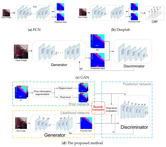
Figure 1.
Framework of several segmentation methods.
2.2. Generative Model
The main purpose of generative model is to produce predicted label graph. The existing methods usually use deep convolutional neural network to obtain the coarse segmentation results, and CRF to refine the results. Although this method can contact the context through CRF, the results of CRF cannot be input to the convolutional neural network to guide the training of network parameters. In CRFAS, the skip connected encoder-decoder network and CRF layer are integrated in the generative model, as shown in Figure 2. After the predicted label graph generated by the generative model is input to the discriminative model, the adversarial loss is utilized to train the network parameters. That is to say, the parameters of gradient back-propagation learning model are calculated based on the results of CRF layer, and the skip connected encoder-decoder structure and CRF layer are a whole network, not CRF as a follow-up optimization independently.
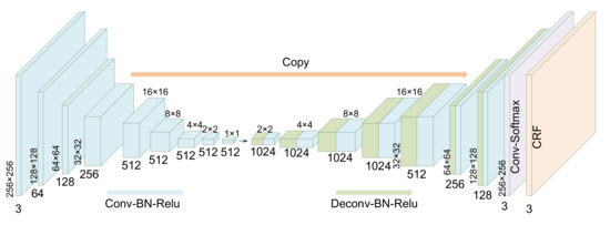
Figure 2.
Structure of generative model.
2.2.1. Conditional Random Fields
Defining a conditional random field on a pixel or an image block can take the segmentation as maximum posteriori problem. CRF contains a smoothness term maximizing the label consistency between similar pixels and describing the context of the pixels. Supposing that image I has P pixels and k categories, the predicted label graph of image I is represented by random field X, , where represents the label of pixel i. Therefore, the segmentation problem can be described as generating a predicted label graph X to maximize the conditional probability , where can be modeled as a conditional random field under Gibbs distribution:
where represents the normalization factor. The energy function can be represented as:
The first item is unitary potential. The unitary potential only considers the category label of each pixel, without considering the information of other pixels. The unitary potential can be obtained by any segmentation models, such as CNNs. The second term is pairwise potential, which represents the joint distribution between the pixel i and pixel j and describes the interaction between the two pixels. For example, pixels with similar colors may belong to the same category. In the fully connected conditional random field, each pixel calculates an energy feature with all other pixels. Thus, the joint energy of all pixels constitutes the pairwise potential energy function, which is represented by weight sums of a series of Gaussian kernels:
Each represents a Gauss kernel function, and M represents the number of kernels. Vectors and represent the eigenvectors of the pixels i and j in any feature space, and denotes the weight of the m-th Gauss kernel. is a label compatibility function, which is usually represented by a Potts model, . This model punishes similar labels with different labels, making pixels with similar characteristics tend to predict the consistency of labels. restricts the conditions of energy transmission, and they can only conduct each other when the labels are identical.
For multi-class image segmentation tasks, the fully connected conditional random fields are usually represented by sensitive binuclear potentials:
and represent color feature vectors. and denote position feature vectors. The first term is appearance kernel function. In this function, pixels with similar color and close spatial distance may belong to the same class, and the degree of proximity of spatial position and similarity of appearance are controlled by and respectively. The second term is the smoothing kernel function, which is used to remove small isolated regions. , , , and are the parameters to be learned in the model.
2.2.2. Unitary Potential
The probabilistic graph predicted by the deep convolutional neural network is used as the unitary potential of CRF in the segmentation network. The network structure of producing unitary potential is unrestricted, which can utilize classical FCN or other deep convolution neural network. To make the input and output images have the same resolution, many models use encoder-decoder structure. In the coding process, a series of convolution and pooling layers reduce the input resolution, and then in the decoding process, the up-sampling layers make the output get the original resolution. In this structure, the high-level features provide semantic information, and the boundary information is gradually recovered during decoding process.
To recover detailed information which losts in the down-sampling process, skip connections are added to the encoder-decoder network [15,16,24,37,38,39]. U-net [16] is a symmetrical U-shaped network, which uses skip connection to combine the feature map of the up-sampling layer from the right expansive path with the feature map of the pooling layer from the left contracting path. Residual encoder-decoder network (RedNet) [39] uses skip connection to bypass the spatial information and proposes fusion structure to introduce depth information into the network. Refs. [24,37] use fully convolutional encoder-decoder structure, and the feature maps of convolution layer are skip-connected to the corresponding deconvolution layer. Learning from [24,37], to connect the encoding part directly to the corresponding decoding part, a skip connection is added between i-th layer and -th layer, as shown in Figure 3. This kind of connection can avoid the bottleneck and directly transmit the shallow layer information to the deep layer, so as to restore the details better. In addition, more detailed information can be obtained by fusing the feature maps of some layers in the network.
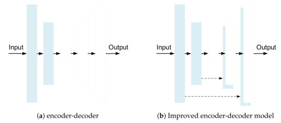
Figure 3.
Improvement in encoder-decoder model.
2.2.3. CRF Layer
Different from the previous separated CRF, referring to the idea of regarding CRF iterative process as recurrent neural network (RNN) [22], one iteration of the mean-field algorithm can be seen as a stack of common CNN layers, then the CRF layer and the convolutional neural network can form an integrated network in our generator. The CRF layer is modeled based on CRF probabilistic graph for structured prediction. The whole generator integrates the advantages of deep convolutional neural network (DCNN) and CRF, and completes end-to-end training through back propagation and random gradient descent. When data passes through the DCNN and enters the CRF layer, the data needs T iterations to leave the cycle created by the CRF layer. The idea of mean field estimation is adopted in the concrete process of CRF layer, but it is implemented in the form of CNN. The structure of CRF layer is shown in Figure 4.
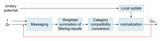
Figure 4.
The iteration in CRF layer.
Each step in mean-field estimation can be realized by the process of CNN: (1) Initialization. The initialization can be completed by softmax. (2) Messaging. The process of messaging is achieved by applying M Gauss filters on Q values. The coefficients of Gauss filter are obtained based on image features, reflecting the correlation between the pixels and other adjacent pixels. Considering that the sensing field of the filter in the fully connected CRF is the whole image, the computational complexity will exceed the expectation. Therefore, the Permutohedral lattice is used to optimize the computation. The Permutohedral lattice can calculate the filter response in time, where P is the number of pixels of the image. (3) Weighted summation of filtering results. The weighted summation of the results of M filters can be regarded as the convolution of the filters with M channels and an output channel. For each class label, the kernel weights are independent of each other and depend on the class label. (4) Category compatibility conversion. The step of class compatibility conversion achieves better results by measuring compatibility between different categories and punishing allocation accordingly. (5) Local updates. The local updating process subtracts the output of the category compatibility conversion from the unitary potential. (6) Normalization. Finally, normalization can be achieved by softmax.
The above is an iteration process of CRF, which can be seen as a stack of common CNN layers. Assuming that the number of iteration is T, the CRF mean field estimation process is executed T times. Each iteration takes estimating from the previous iteration as , and input into this iteration with unitary potential and the input image I. This iterative mean-field inference can be seen as a RNN.
2.3. Discriminative Model
The discriminative model can adopt models with different output structures. In the atomic level, the discriminator determines the image in a pixel manner, called PixelGAN. The discriminative model judges the image in the image level, called ImageGAN. Between the two levels, there is the patch level, where the discriminative model makes decisions in patch, called PatchGAN [40].
PatchGAN divides the input into several patches. The discriminative model determines the authenticity of each patch, and takes the average of all patch outputs as the final output of the discriminative model. The structure is punished on the scale of patch, and the size K of patch is much smaller than that of image. The smaller patchGAN has fewer parameters, runs faster and can be applied to any size image.
Among the existing structures, cross-entropy loss can restrict the pixel-level correctness of the image, therefore, it is not necessary to emphasize the pixel-level correctness in the design of the discriminative model, but should pay attention to the simulation of region-level structure. For the above reasons, PatchGAN is adopted as the discriminative model. The structure of discriminative model is shown in Figure 5. Three convolution-batchnorm-relu layers are followed by a max pooling layer, then two convolution-batchnorm-relu layers are connected with a max pooling layer, followed by a convolution-batchnorm-relu layer. Finally, a distribution map is generated through a convolution-sigmoid layer. The discriminator can determine whether the input image is a predicted label graph or a ground truth by calculating the mean of distribution map.
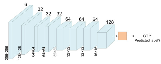
Figure 5.
Structure of discriminative model.
2.4. Loss Function
To improve the segmentation accuracy, the loss function combines the cross-entropy loss at the pixel level and the adversarial loss at the region level. The loss function is defined as:
where and represent the parameters of generator and discriminator respectively. is the cost function of the classical segmentation method, such as cross-entropy, which is the negative logarithm of probability value. The loss is generated by calculating the differences between the predicted label graph and the ground truth pixel by pixel. denotes the objective of a conditional GAN. It is defined as the cost of predicted label graph to be detected by the discriminative model. The discriminative model considers whether the predicted label graph is similar to the ground truth or not. In the discriminative model, the convolution and pooling layers can obtain the context information in a certain area, which makes up for the defect that classical cost function does not consider structure information. is distance, which is used to make the predicted label graph as similar as the ground truth. Weight is used to balance the two kinds of losses. The data set has N training images. represents the original image, represents the ground truth, and denotes the predicted label graph. Since the cross-entropy loss lacks spatial structure information, and adversarial loss only considers high-order consistency. By combining cross-entropy loss and adversarial loss, we take advantages of both to compensate for their shortcomings.
In the training process, the parameters of discriminative model and the parameters of generative model are alternately trained. The cost function used to train the discriminative model is as follows:
In the above formula, . The first part of the formula represents that the ground truth is judged to be 1, and the second part represents that the predicted label graph is judged to be 0 in the discriminative model. These two parts reflect the ability of the discriminative model to distinguish the ground truth and the predicted label graph. By minimizing the function, the best performance of the discriminative model can be obtained. The cost function used to train the generative model is:
The first part in the formula is cross-entropy loss, which calculates the difference between the ground truth and the predicted label graph at the pixel level. , where P represents the pixel numbers of predicted label graph. The third part is the adversarial loss. If the discriminative model recognizes the predicted label graph, the predicted label generated by the generative model is not good. Thus, the loss function increase. It is hoped that when the generative model is fully trained, the discriminative model cannot distinguish between ground truth and the predicted label.
2.5. Model Training
In the model training process, the generative model and the discriminative model are trained alternately after each gradient descent step. To avoid the imbalance between the two models caused by the strong discriminative model, the optimization goal of the discriminative model is divided by two to reduce the learning speed of the adversarial network. Since cannot provide enough gradient in training and generative model, there will be obvious difference between the predicted label graph and the ground truth in the initial stage, the discriminative model can easily identify the predicted label graph, thus, the loss of the discriminative model will be saturated. To solve this problem, we follow Luc et al. [23] to use to replace in the process of training the generative model, that is to say, the probability of identifying as a predicted label graph by minimizing the discriminative model is replaced by the probability of identifying as ground truth by maximizing the discriminative model. The critical points of these two probabilities are the same, but the discriminative model will produce stronger gradient signals when it makes more accurate judgements, which can accelerate the early learning. Mini-batch random gradient descent and ADAM are used to solve this problem. The learning rate is set to 0.0002 and the momentum parameter are set to , . The epochs of two data sets are 400 and 53 respectively.
3. Flowchart
The network structure of CRFAS for training and testing is shown in Figure 6. Figure 6a shows the network structure in training process, where the structure is divided into two modules: the generative model and the discriminative model. The generative model segments the input image to obtain the predicted label graph. The internal structure of the generative model consists of an integrated skip connected encoder-decoder network and a CRF layer. The deep convolutional neural network segments the image into a rough segmented probability map, and the map is regarded as an unitary potential in CRF. Then, in CRF layer, the pairwise potential is constructed according to the label relationship between pixels, and iteratively optimized with the unitary potential to obtain the predicted label. The predicted label graph and the prior information output by the prior network are jointly input into the discriminative model, and the output probability value of the discriminative model indicates the similarity between the predicted label graph and the ground truth. According to the probability value of the output, the adversarial loss can be calculated, and then the gradient inversion is carried out to train the parameters of each module by combining the prediction of the cross-entropy loss between the predicted label graph and the pixel-level prior information. Figure 6b shows the network structure in testing process. When the training is completed, the parameters of the generative model are fixed. Thus, the discriminative model does not participate in the testing process. The image is input into the generative model, and then the rough probability map generated by the deep convolutional neural network is input into CRF layer as the unitary potential. Finally, the segmentation result is obtained.
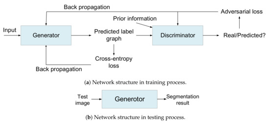
Figure 6.
Flowchart of training and testing process.
4. Experiment
4.1. Experiment Data
To evaluate the validity of our proposed method, experiments were carried out on two data sets. The first set of data is E-SAR L-band PolInSAR image of the German Aerospace Center, which contains many typical characteristics, such as roads, buildings and forests. The resolution of the data is 3 m × 3 m, the size of original image is , and the intercepted image is pixels. The interested areas can be divided into five categories: road, farmland, building, forest and other land cover. The PauliSAR image and its ground truth are shown in Figure 7.
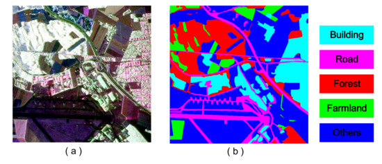
Figure 7.
The experimental data 1. (a) Pauli SAR image; (b) The ground truth.
To use all the information in the training process, the image was divided into four blocks, three of which were trained in each experiment and one was used for testing. Since the data set is small, following [41,42,43], we have not set a validation set in order to ensure adequate training. Then, four times of training were carried out to get four similar models and corresponding test pictures. Finally, the final test results were obtained by combining four test pictures. The size of small image is , the sampling interval is 49 pixels, and a large image can be divided into 400 small images. Compared with ordinary optical images, remote sensing images have multi-directional characteristics. To increase the multi-directionality of training, a series of methods were adopted to increase the direction diversity of training data. The expansion was mainly carried out by two methods: inversion and rotation.
The second data set is GID, which is a high-resolution data set for land classification proposed by Tong et al. [44]. The GF-2 images in GID were acquired from 5 December 2014 to 13 October 2016. Five categories are marked in different colors: building (red), farmland (green), forest (cyan), grassland (yellow) and water area (blue). Areas that do not belong to the above five categories or cannot be artificially identified are marked black. One example of original images and its ground truth are shown in Figure 8.
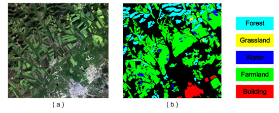
Figure 8.
The experimental data 2. (a) Remote sensing image; (b) The ground truth.
There are 150 large images in data set 2, the size of each image is pixels. We took 120 images as training set, 15 as validation set and 15 as test set. For each large image, 783 small images with pixels were cut without overlap. For the test set, each large image was cut to small images as the test samples which are input into the trained model to get the predicted label graphs, and the small graphs were spliced into a large one to get the final segmentation result.
4.2. Experiment Result
The segmentation results of our proposed method are compared with three segmentation algorithms: (1) FCN; (2) Deeplab; (3) Pixel2pixel [24]. The first comparison algorithm, FCN, is the pioneering work of semantic segmentation network. Deeplab is chosen to be the second comparison algorithm since it proposes atrous convolution and utilizes the fully connected CRF for post-optimization. The third comparison method is Pixel2pixel, which is based on generative adversarial network.
The segmentation results conducted on data set 1 with these four methods are shown in Figure 9.
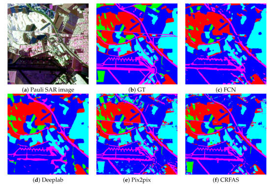
Figure 9.
Segmentation results 1.
Three examples of the segmentation results conducted on data set 2 with these four methods are shown in Figure 10, Figure 11 and Figure 12. Image 1, 2, 3 contains 5, 4, 3 data categories, respectively.
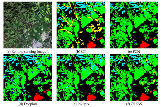
Figure 10.
Segmentation results 2.
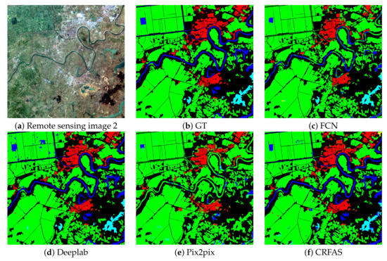
Figure 11.
Segmentation results 3.
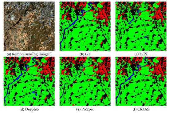
Figure 12.
Segmentation results 4.
To evaluate the model proposed in this paper quantitatively, the following three evaluation indicators are used: (1) The confusion matrix and overall accuracy. (2) F1 score. (3) Mean Intersection over Union (MIoU).
4.2.1. The Confusion Matrix and Overall Accuracy
To quantitatively evaluate the segmentation accuracy of each category, the confusion matrix of data set 1 is shown in Table 1. For each category, the ratio of the number of correctly classified pixels in the segmentation result to the total number of all the pixels in the ground truth is calculated. The overall segmentation accuracy calculates the average accuracy of all categories. In the calculating process, the background part is removed and the segmentation accuracy of the remaining part is calculated. The calculation method is as follows: after removing the background part, the ratio of the correct classified pixels in the segmentation result to the total number of pixels in the ground truth is calculated. Table 2, Table 3 and Table 4 show the confusion matrices of three example images of data set 2.

Table 1.
Confusion Matrix of data set 1.
Table 2.
Confusion Matrix of image 1.
Table 3.
Confusion Matrix of image 2.
Table 4.
Confusion Matrix of image 3.
After observing the above four confusion matrixes, it can be seen that CRFAS has the highest overall accuracy and good robustness. For data set 1, compared with Deeplab, CRFAS has higher accuracy in road and farmland categories. The confusion matrix of the complete data set 2 is shown in Table 5. From Table 5, it can be seen that CRFAS has the highest overall accuracy and good performance in farmland, water, and building categories. For forest category, the accuracy of CRFAS is not as good as Deeplab’s. These four methods did not perform well in grassland category.
Table 5.
Confusion Matrix of Data Set 2.
In terms of overall accuracy, CRFAS has better segmentation results than FCN, Deeplab and Pixel2pixel. To further compare the segmentation results of our proposed method with three other algorithms, the F1 score and mIoU are calculated in the following.
4.2.2. F1 Score and mIOU
The calculation of F1 score is based on recall and precision. The formulations are as follows:
where represents true positive, which is the number of pixels in the category for both the predicted result and the real label. represents false positive, which is the number of pixels predicted for each category but not for the real label. represents false negative, which is the number of pixels in each category that are not predicted label but are real label as such.
The precision and recall are contradictory measures. Generally, when the precision is high, the recall is low, while when the recall is high, the precision is low. For example, if the segmentation results of a category are expected to have a high accuracy, pixels can be classified into this category as many as possible. If the whole images is classified into this category, the pixels belonging to this category in the label graph must be correctly classified, in which way the precision will be very low, and vice versa. Therefore, we hope to find a balance point between precision and recall. F1 score is an evaluation metric used to balance precision and recall. The calculation formulation is as follows:
F1 score is the harmonic average of precision and recall, which reflects the relative double-high degree of precision and recall of model segmentation results to a certain extent. The higher the score of F1, the more reliable the segmentation result is.
Mean intersection over union (MIoU) is a standard measure of semantic segmentation. Intersection over union (IoU) calculates the ratio of the intersection and union of two classifications. IoU is calculated on each class and then mIOU is obtained. MIoU can be calculated by the following:
where represents the number of pixels in which the predicted label and the real label are i.
The F1 score and mIOU of data set 1 are shown in Table 6. Table 7 displays the F1 score and mIoU of three example images and the evaluation results of complete data set 2.
Table 6.
F1 score and mIoU of Data Set 1.
Table 7.
F1 score and mIoU of Data Set 2.
For data set 1, CRFAS has higher mIoU than three other comparison methods. In terms of F1 score, CRFAS maintains a better balance between precision and recall than the other three methods.
As can be seen from Table 7, CRFAS has the highest mIoU among four methods for data set 2. We compare segmentation results of these four methods in details. In image 1, four methods have low F1 score in water and grassland categories. Deeplab has better performance than CRFAS in farmland and building categories. However, for farmland, water, and building categories in image 2 and image 3, CRFAS has highest F1 score. For complete data set 2, CRFAS has the highest mIoU and performs best in three categories: farmland, water and building.
4.3. Discussion
Three evaluation indexes are synthesized to evaluate the segmentation results. The segmentation results of CRFAS on two data sets have the highest overall accuracy and mIoU among the four algorithms. Comparing the precision and F1 score of each category, for data set 1, we can see that CRFAS has obvious advantages. For data set 2, as shown in Figure 13, CRFAS has the highest precision and F1 score in farmland, water and building categories. In the forest category, FCN and Deeplab have higher precision and F1 score than CRFAS. For the grassland category, these four methods perform poorly in terms of precision and F1 score.
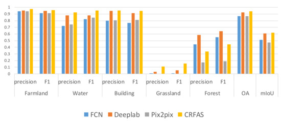
Figure 13.
Statistics on the evaluation indexes of Data Set 2.
Based on the experimental results, three main contributions of the proposed method can be summarized as follows.
- (1)
- A conditional generative adversarial segmentation network is proposed based on the Bayesian framework. The networks joint training and adversarial learning make the segmentation results as close as possible to the ground truth. While FCN is a segmentation network, and Deeplab adds conditional random fields as post-processing after segmentation network. We directly observe the segmented results and can see that at the lower part of Figure 12, FCN and Deeplab labeled farmland as water, but CRFAS and pixel2pixel did not.
- (2)
- To obtain details and consider global information, the skip-connected encoder-decoder architecture is integrated with CRF layer to form an end-to-end generative model, so as to improve the accuracy of segmentation. FCN8 and Pixel2pixel use skip connections between different layers to get detailed information, but the global information is not taken into account. Observing the segmentation results directly, it can be seen that in Figure 11 and Figure 12, CRFAS and Deeplab succeeded in segmenting rivers (blue), while FCN and pixel2pixel failed.
- (3)
- A new loss function including the cross-entropy loss and the adversarial loss is defined to guide the training of the whole segmentation network. In contrast, FCN and Deeplab only consider the difference of each pixel to calculate the cross-entropy loss, while pixel2pixel does not take the pixel-level difference into account. Combined with the above, for these two data sets, CRFAS completes the segmentation task and has highest accuracy and mIoU among the four semantic segmentation methods.
However, our proposed method still has some shortcomings. The main shortcoming is that CRFAS does not perform well in categories with fewer training samples, such as forest category in data set 2. Second, our proposed method takes a long time to train the model. The training time consumed in training data set 1 is counted in Table 8. Our future work will focus on improving accuracy of small sample categories and computational efficiency.
Table 8.
Training time of data set 1.
5. Conclusions
In this paper, a new end-to-end semantic segmentation model called CRFAS is proposed. In CRFAS algorithm, the CRF is combined with GAN in a Bayesian framework. The adversarial loss and the cross-entropy loss are utilized to guide the training process through back propagation. The algorithm mainly relies on three factors. First, the generative adversarial network and Bayesian framework are combined to realize the estimation from the prior probability to the posterior probability. Second, the generative model takes details and global information into consideration by integrating the skip-connected encoder-decoder structure and CRF layer. Finally, the loss function redefined is utilized to guide the training process of the whole model. The experimental results show that our proposed method can achieve semantic segmentation and have good performance. However, long training time and low accuracy of small sample categories are limitations of our proposed method. Our future work will mainly focus on improving the accuracy of small samples and reducing training time.
Author Contributions
C.H. and P.F. conceived and designed the experiments; Z.Z. performed the experiments and analyzed the results; C.H. and P.F. wrote the paper; D.X. and M.L. revised the paper.
Acknowledgments
This work was supported by the National Natural Science Foundation of China (No.61331016, No.41371342), the National Key Research and Development Program of China (No. 2016YFC0803000), and the Hubei Innovation Group (2018CFA006).
Conflicts of Interest
The authors declare no conflict of interest.
References
- Li, D.; Zhang, G.; Wu, Z.; Yi, L. An edge embedded marker-based watershed algorithm for high spatial resolution remote sensing image segmentation. IEEE Trans. Image Process. 2010, 19, 2781–2787. [Google Scholar] [PubMed]
- Zhang, X.; Xiao, P.; Feng, X.; Wang, J.; Zuo, W. Hybrid region merging method for segmentation of high-resolution remote sensing images. ISPRS J. Photogramm. Remote Sens. 2014, 98, 19–28. [Google Scholar] [CrossRef]
- Girshick, R.; Donahue, J.; Darrell, T.; Malik, J. Region-based convolutional networks for accurate object detection and segmentation. IEEE Trans. Pattern Anal. Mach. Intell. 2016, 38, 142–158. [Google Scholar] [CrossRef] [PubMed]
- Zhu, X.X.; Tuia, D.; Mou, L.; Xia, G.S.; Fraundorfer, F. Deep Learning in Remote Sensing: A Comprehensive Review and List of Resources. IEEE Geosci. Remote Sens. Mag. 2018, 5, 8–36. [Google Scholar] [CrossRef]
- Maggiori, E.; Tarabalka, Y.; Charpiat, G.; Alliez, P. Convolutional Neural Networks for Large-Scale Remote Sensing Image Classification. IEEE Trans. Geosci. Remote Sens. 2016, 55, 645–657. [Google Scholar] [CrossRef]
- Simonyan, K.; Zisserman, A. Very Deep Convolutional Networks for Large-Scale Image Recognition. Comput. Sci. 2014, arXiv:1409.1556. [Google Scholar]
- He, K.; Zhang, X.; Ren, S.; Sun, J. Deep residual learning for image recognition. In Proceedings of the IEEE Conference on Computer Vision and Pattern Recognition, Las Vegas, NV, USA, 27–30 June 2016; pp. 770–778. [Google Scholar]
- Noh, H.; Hong, S.; Han, B. Learning deconvolution network for semantic segmentation. In Proceedings of the IEEE International Conference on Computer Vision, Santiago, Chile, 7–13 December 2015; pp. 1520–1528. [Google Scholar]
- Peng, C.; Zhang, X.; Yu, G.; Luo, G.; Sun, J. Large Kernel Matters–Improve Semantic Segmentation by Global Convolutional Network. In Proceedings of the IEEE Conference on Computer Vision and Pattern Recognition, Honolulu, HI, USA, 21–26 July 2017; pp. 4353–4361. [Google Scholar]
- Nogueira, K.; Miranda, W.O.; Dos Santos, J.A. Improving spatial feature representation from aerial scenes by using convolutional networks. In Proceedings of the 2015 28th SIBGRAPI Conference on Graphics, Patterns and Images, Salvador, Brazil, 26–29 August 2015; pp. 289–296. [Google Scholar]
- Jia, Y.; Shelhamer, E.; Donahue, J.; Karayev, S.; Long, J.; Girshick, R.; Guadarrama, S.; Darrell, T. Caffe: Convolutional architecture for fast feature embedding. In Proceedings of the 22nd ACM International Conference on Multimedia, Orlando, FL, USA, 3–7 November 2014; pp. 675–678. [Google Scholar]
- Sermanet, P.; Eigen, D.; Zhang, X.; Mathieu, M.; Fergus, R.; LeCun, Y. Overfeat: Integrated recognition, localization and detection using convolutional networks. arXiv Preprint, 2013; arXiv:1312.6229. [Google Scholar]
- Krizhevsky, A.; Sutskever, I.; Hinton, G.E. Imagenet classification with deep convolutional neural networks. In Proceedings of the Advances in Neural Information Processing Systems, Lake Tahoe, NV, USA, 3–6 December 2012; pp. 1097–1105. [Google Scholar]
- Long, J.; Shelhamer, E.; Darrell, T. Fully Convolutional Networks for Semantic Segmentation. In Proceedings of the The IEEE Conference on Computer Vision and Pattern Recognition (CVPR), Boston, MA, USA, 7–12 June 2015. [Google Scholar]
- Badrinarayanan, V.; Kendall, A.; Cipolla, R. Segnet: A deep convolutional encoder-decoder architecture for image segmentation. IEEE Trans. Pattern Anal. Mach. Intell. 2017, 39, 2481–2495. [Google Scholar] [CrossRef]
- Ronneberger, O.; Fischer, P.; Brox, T. U-net: Convolutional networks for biomedical image segmentation. International Conference on Medical Image Computing and Computer-Assisted Intervention; Springer: Cham, Switzerland, 2015; pp. 234–241. [Google Scholar]
- Chen, L.C.; Papandreou, G.; Kokkinos, I.; Murphy, K.; Yuille, A.L. Deeplab: Semantic image segmentation with deep convolutional nets, atrous convolution, and fully connected crfs. IEEE Trans. Pattern Anal. Mach. Intell. 2018, 40, 834–848. [Google Scholar] [CrossRef]
- Zhao, H.; Shi, J.; Qi, X.; Wang, X.; Jia, J. Pyramid Scene Parsing Network. arXiv, 2016; arXiv:1612.01105. [Google Scholar]
- Krähenbühl, P.; Koltun, V. Efficient inference in fully connected crfs with gaussian edge potentials. In Proceedings of the Advances in Neural Information Processing Systems, Granada, Spain, 12–15 December 2011; pp. 109–117. [Google Scholar]
- Liu, F.; Lin, G.; Shen, C. CRF learning with CNN features for image segmentation. Pattern Recognit. 2015, 48, 2983–2992. [Google Scholar] [CrossRef]
- Liu, F.; Lin, G.; Shen, C. Discriminative training of deep fully connected continuous CRFs with task-specific loss. IEEE Trans. Image Process. 2017, 26, 2127–2136. [Google Scholar] [CrossRef] [PubMed]
- Zheng, S.; Jayasumana, S.; Romera-Paredes, B.; Vineet, V.; Su, Z.; Du, D.; Huang, C.; Torr, P.H. Conditional random fields as recurrent neural networks. In Proceedings of the IEEE International Conference on Computer Vision, Santiago, Chile, 7–13 December 2015; pp. 1529–1537. [Google Scholar]
- Luc, P.; Couprie, C.; Chintala, S.; Verbeek, J. Semantic segmentation using adversarial networks. arXiv Preprint, 2016; arXiv:1611.08408. [Google Scholar]
- Isola, P.; Zhu, J.Y.; Zhou, T.; Efros, A.A. Image-to-image translation with conditional adversarial networks. In Proceedings of the IEEE Conference on Computer Vision and Pattern Recognition, Honolulu, HI, USA, 21–26 July 2017; pp. 1125–1134. [Google Scholar]
- Zhu, W.; Xiang, X.; Tran, T.D.; Xie, X. Adversarial deep structural networks for mammographic mass segmentation. arXiv Preprint, 2016; arXiv:1612.05970. [Google Scholar]
- Ma, F.; Gao, F.; Sun, J.; Zhou, H.; Hussain, A. Weakly Supervised Segmentation of SAR Imagery Using Superpixel and Hierarchically Adversarial CRF. Remote Sens. 2019, 11, 512. [Google Scholar] [CrossRef]
- Souly, N.; Spampinato, C.; Shah, M. Semi supervised semantic segmentation using generative adversarial network. In Proceedings of the IEEE International Conference on Computer Vision, Honolulu, HI, USA, 21–26 July 2017; pp. 5688–5696. [Google Scholar]
- Fu, C.; Lee, S.; Joon Ho, D.; Han, S.; Salama, P.; Dunn, K.W.; Delp, E.J. Three dimensional fluorescence microscopy image synthesis and segmentation. In Proceedings of the IEEE Conference on Computer Vision and Pattern Recognition Workshops, Salt Lake City, UT, USA, 18–22 June 2018; pp. 2221–2229. [Google Scholar]
- Huo, Y.; Xu, Z.; Bao, S.; Bermudez, C.; Plassard, A.J.; Liu, J.; Yao, Y.; Assad, A.; Abramson, R.G.; Landman, B.A. Splenomegaly segmentation using global convolutional kernels and conditional generative adversarial networks. SPIE Proc. 2018, 10574, 1057409. [Google Scholar]
- Hariharan, B.; Arbelaez, P.; Girshick, R.; Malik, J. Hypercolumns for Object Segmentation and Fine-Grained Localization. In Proceedings of the The IEEE Conference on Computer Vision and Pattern Recognition (CVPR), Boston, MA, USA, 7–12 June 2015. [Google Scholar]
- Kluckner, S.; Bischof, H. Semantic classification by covariance descriptors within a randomized forest. In Proceedings of the 2009 IEEE 12th International Conference on Computer Vision Workshops, ICCV Workshops, Kyoto, Japan, 27 September–4 October 2009; pp. 665–672. [Google Scholar]
- Li, W.; He, C.; Fang, J.; Zheng, J.; Fu, H.; Yu, L. Semantic Segmentation-Based Building Footprint Extraction Using Very High-Resolution Satellite Images and Multi-Source GIS Data. Remote Sens. 2019, 11, 403. [Google Scholar] [CrossRef]
- Zhang, Z.; Wang, Y. JointNet: A Common Neural Network for Road and Building Extraction. Remote Sens. 2019, 11, 696. [Google Scholar] [CrossRef]
- Papadomanolaki, M.; Vakalopoulou, M.; Karantzalos, K. A Novel Object-Based Deep Learning Framework for Semantic Segmentation of Very High-Resolution Remote Sensing Data: Comparison with Convolutional and Fully Convolutional Networks. Remote Sens. 2019, 11, 684. [Google Scholar] [CrossRef]
- Panboonyuen, T.; Jitkajornwanich, K.; Lawawirojwong, S.; Srestasathiern, P.; Vateekul, P. Semantic Segmentation on Remotely Sensed Images Using an Enhanced Global Convolutional Network with Channel Attention and Domain Specific Transfer Learning. Remote Sens. 2019, 11, 83. [Google Scholar] [CrossRef]
- Pan, X.; Gao, L.; Marinoni, A.; Bing, Z.; Gamba, P. Semantic Labeling of High Resolution Aerial Imagery and LiDAR Data with Fine Segmentation Network. Remote Sens. 2018, 10, 743. [Google Scholar] [CrossRef]
- Mao, X.; Shen, C.; Yang, Y.B. Image restoration using very deep convolutional encoder-decoder networks with symmetric skip connections. In Proceedings of the Advances in Neural Information Processing Systems, Barcelona, Spain, 5–10 December 2016; pp. 2802–2810. [Google Scholar]
- Kumar, P.; Nagar, P.; Arora, C.; Gupta, A. U-Segnet: Fully Convolutional Neural Network Based Automated Brain Tissue Segmentation Tool. In Proceedings of the 2018 25th IEEE International Conference on Image Processing (ICIP), Athens, Greece, 7–10 October 2018; pp. 3503–3507. [Google Scholar]
- Jiang, J.; Zheng, L.; Luo, F.; Zhang, Z. Rednet: Residual encoder-decoder network for indoor rgb-d semantic segmentation. arXiv Preprint, 2018; arXiv:1806.01054. [Google Scholar]
- Son, J.; Park, S.J.; Jung, K.H. Retinal vessel segmentation in fundoscopic images with generative adversarial networks. arXiv Preprint, 2017; arXiv:1706.09318. [Google Scholar]
- Liu, Y.; Fan, B.; Wang, L.; Bai, J.; Xiang, S.; Pan, C. Semantic labeling in very high resolution images via a self-cascaded convolutional neural network. ISPRS J. Photogramm. Remote Sens. 2018, 145, 78–95. [Google Scholar] [CrossRef]
- Wei, X.; Guo, Y.; Gao, X.; Yan, M.; Sun, X. A new semantic segmentation model for remote sensing images. In Proceedings of the 2017 IEEE International Geoscience and Remote Sensing Symposium (IGARSS), Fort Worth, TX, USA, 23–28 July 2017; pp. 1776–1779. [Google Scholar]
- Cheng, W.; Yang, W.; Wang, M.; Wang, G.; Chen, J. Context Aggregation Network for Semantic Labeling in Aerial Images. Remote Sens. 2019, 11, 1158. [Google Scholar] [CrossRef]
- Tong, X.; Xia, G.; Lu, Q.; Shen, H.; Li, S.; You, S.; Zhang, L. Learning Transferable Deep Models for Land-Use Classification with High-Resolution Remote Sensing Images. arXiv Preprint, 2018; arXiv:1807.05713. [Google Scholar]


© 2019 by the authors. Licensee MDPI, Basel, Switzerland. This article is an open access article distributed under the terms and conditions of the Creative Commons Attribution (CC BY) license (http://creativecommons.org/licenses/by/4.0/).