Abstract
The estimation of aboveground biomass (AGB), an important indicator of grassland production, is crucial for evaluating livestock carrying capacity, understanding the response and feedback to climate change, and achieving sustainable development. Most existing grassland AGB estimation studies were based on empirical methods, in which field measurements are indispensable, hindering their operational use. This study proposed a novel physically-based grassland AGB retrieval method through the inversion of PROSAIL model against MCD43A4 imagery. This method relies on the basic understanding that grassland is herbaceous, and therefore AGB can be represented as the product of leaf dry matter content (Cm) and leaf area index (LAI), i.e., AGB = Cm × LAI. First, the PROSAIL model was parameterized according to the literature regarding grassland parameters retrieval, then Cm and LAI were retrieved using a lookup table (LUT) algorithm, finally, the retrieved Cm and LAI were multiplied to obtain the AGB. The method was assessed in Zoige Plateau, China. Results show that it could reproduce the reference AGB map, which is generated by upscaling the field measurements, in terms of magnitude (with RMSE and R-RMSE of 60.06 g·m−2 and 18.1%, respectively) and spatial distribution. The estimated AGB time series also agreed reasonably well with the expected temporal dynamic trends of the grassland in our study area. The greatest advantage of our method is its fully physical nature, i.e., no field measurement is needed. Our method has the potential for operational monitoring of grassland AGB at regional and even larger scales.
1. Introduction
Grassland, defined as permanent vegetation of herbaceous plant communities, provides significant ecosystem services, carbon pooling, and forage production [1,2,3]. Aboveground biomass (AGB), which is defined as the total mass of plant material per unit area, is an important indicator of vegetation production. The estimation of grassland AGB is therefore crucial for evaluating livestock carrying capacity, understanding the response and feedback to climate change, and achieving sustainable development [4,5].
The traditional method to estimate grassland AGB is based on field measurement, consisting of field clippings, laboratory drying, and weighing [4]. Although the field measurement methods are accurate, they are time-consuming and labor-intensive. In addition, their spatially sparse nature makes them unfeasible to give a comprehensive understanding at regional or larger scales [6]. Optical remote sensing data contain valuable information on vegetation parameters, and therefore provide an alternative to monitor grassland AGB more handily and in a seamless manner [7].
Various methods have been developed for estimating grassland AGB from optical remote sensing data, and most of them are by nature empirical, and based on transfer functions between AGB and remote sensing observation [1,8,9,10,11]. Transfer functions can be parametric (e.g., linear [2,12], exponential [8], and power fitting [5]) or non-parametric (e.g., support vector machine [13] and artificial neural network [14]). Field measurements are also indispensable in these empirical methods to calibrate the transfer functions. Limited by the representativeness of the field measurements, the resulting transfer function is often time-, site-, and sensor-specific. Therefore, corresponding field measurements should be implemented beforehand, and these empirical methods are also time consuming and labor intensive.
Canopy radiative transfer models summarize our understanding regarding the photon–canopy interaction and establish the explicit physical relation between vegetation parameters and remote sensing observations [15,16,17]. The robustness and transferability of radiative transfer models makes them a preferable solution to the abovementioned condition-specific problem. Physically-based methods by inverting canopy radiative transfer models have been extensively used to retrieve leaf area index, fraction of absorbed photosynthetic active radiation, fraction of green vegetation cover, and many other parameters [18,19]. However, the physically-based method to retrieve AGB is still at its infancy. One major reason is the lack of a proper radiative transfer model to account for the pool of canopy dry matter constituting the AGB. For example, the primary pool of forest AGB is the tree trunk, yet there is no single radiative transfer model accounting for its dry weight. However, there is no such predicament for grassland considering its herbaceous nature. The dry matter of grassland is mostly from the leaves (i.e., leaf dry matter content, Cm), and significantly determining the leaf spectrum, which can be described by leaf optical models (e.g., the PROSPECT model [20]). In addition, the amount of the leaves can also be depicted by leaf area index, which is an important input of many canopy scale models, such as SAILH [21]. Therefore, a physically-based model to retrieve grassland AGB is possible, given the fact that grassland AGB is the product of leaf dry matter content and leaf area index (AGB = Cm × LAI).
Very few pioneers of physically-based methods for grassland AGB found are in literature, including Punalekar’s [22] and Quan’s [23] study. They were both based on PROSAIL model [20,21], which achieved an appropriate compromise between simulating accuracy and inverting simplification. Punalekar et al. [22] firstly retrieved LAI by inverting PROSAIL model, then converted the LAI into AGB through a constant value of Cm estimated through field measurement. In fact, Cm is a spatiotemporal variable [24,25], so its constant assumption may cause uncertainty for the retrieved AGB. In contrast, Quan et al [23] simultaneously retrieved the LAI and Cm from PROSAIL model, and then obtained the final AGB through multiplying these two variables. Yet, an empirical relationship between leaf equivalent water thickness and Cm was used in their study, which may reduce the generality of their method. A re-calibration of their method is also needed, when applied to different scenarios or time frames. In summary, empirical variables or relationships are still involved in existing physically-based method, and a fully physically-based method for grassland AGB retrieval method still does not exist.
Different data sources were employed to mapping grassland AGB, e.g., Landsat [14,23], SPOT [1], MERIS [26], and Sentinel [27,28]. The long-term coverage and high revisiting frequency make MODIS an unparalleled data source, and it has been widely used in grassland AGB estimation [2,13,28,29]. However, the performance of physically-based method on MODIS data has not been assessed. A fully physically-based method for grassland AGB retrieval from MODIS imagery is urgently needed to further improve the accuracy and spatiotemporal coverage of grassland AGB estimation.
The objective of this study is to propose a physically-based method to estimate grassland AGB based on inverting the PROSAIL model from MODIS data. The proposed method relies on the basic understanding that grassland is herbaceous, and therefore AGB can be represented as the product of Cm and LAI, i.e., AGB = Cm × LAI. The main improvement of our method is its independence from any field measurement, i.e., it is a fully physically-based method, and no empirical variable or relationship is needed. Performances of the proposed method were evaluated in the Zoige Plateau, China.
2. Materials and Methods
2.1. Study Area
This study was implemented in a 100 × 100 km region spanning from the upper-left corner at 34.0° N and 102.4° E to the bottom-right corner at 33.1° N and 103.5° E in the Zoige Plateau (Figure 1). This region is located at the junction of Sichuan, Gansu and Qinghai provinces, China. The top three dominant land covers are grassland (80.8%), wetland (11.1%), and forest (4.2%) [6] according to the European Space Agency Climate Change Initiative (CCI) project (available at http://maps.elie.ucl.ac.be/CCI/viewer/download.php). The average elevation of the study area is ~ 3400 m above sea level. The study area is characterized by low temperature (with an annual mean temperature of 1.21°C) and high humidity (with annual precipitation ranging from 464.8 to 862.9 mm) [30].
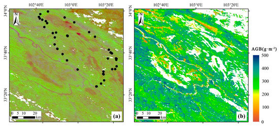
Figure 1.
Study area. (a) MCD43A4 image from August 13, 2017 (the R, G, and B color space correspond to bands 6, 2, and 1, respectively). Sampling plots for the field aboveground biomass measurements are displayed as black dots. (b) is the reference aboveground biomass (AGB) map used to validate the proposed method. The white pixels in (a,b) are bad-quality and non-grassland pixels, respectively. For details regarding the generation of (b), please see [6].
2.2. Data
2.2.1. Field Measurements and Reference AGB Map
A field campaign was implemented from 14 to 19 August (day of year, DOY 226-231), 2017. Forty-four plots with areas of 100 × 100 m were selected to perform the field measurement (Figure 1a). In each plot, three 0.5 × 0.5 m quadrats were selected. All plants in each quadrat were clipped at the ground surface, transported to the laboratory, and oven-dried at 80 °C for 48 hours until a constant dry biomass was obtained. The average AGB value of the three quadrats within one plot was used to represent the AGB at the plot scale. Landsat 8 Operational Land Imager (OLI) data was then involved in upscaling the sparse field measurements to a seamless AGB map (Figure 1b). The consistent adjustment of the climatology to actual observations (CACAO) method and Gaussian process regression (GPR) were employed, during the upscaling process, to copy with the spatial gaps that exist in the OLI data and fully exploit the multispectral data cube, respectively. The details regarding the field measurement and AGB mapping can be found in [6].
The AGB map mentioned above was generated from field measurements and was seen as ‘true values’ to validate the physically-based method in this study.
2.2.2. MODIS Nadir BRDF-Adjusted Reflectance
In this study, MODIS 16-day nadir BRDF-Adjusted Reflectance product (MCD43A4) was used to estimate grassland AGB. MCD43A4 is computed for each of the MODIS spectral bands (1–7, see Table 1) as if they were taken from the nadir view at local solar noon of the day [31]. Both Terra and Aqua data from a 16-day period were used to provide highest quality input data. Since the view angle effects are removed from the reflectance observations, this will facilitate the subsequent applications considering the stability and consistence of the angularly normalized reflectance.

Table 1.
Band specification of the MCD43A4 products
Forty-six images with tile of h26v05 were downloaded from the Land Processes Distributed Active Archive Center (LPDAAC). These images were from DOY 1 to 361 in 2017 with an 8 days step. We did not use daily V6 MCD43A4 images directly, because the temporally adjacent images have too much temporal overlapping considering the 16-day compositing window, and this results in the temporally adjacent images revealing very slight discrepancies.
The incidence angle of the MCD43A4 product has been normalized to local solar noon of the day, which will change across the study year (2017). Yet, the local solar noon zenith angle within the study area would not cover too wide range, considering the limited space of our study area (Figure 1). Therefore, the incidence angle of the central pixel can be safely use to represent the entire study area. Figure 2 illustrates the temporal variation of the incidence zenith angle for the central pixel computed using an astronomical model [32]. The incidence angle is very oblique during winter: the incidence zenith angle is more than 50° at the beginning and ending of the study year. Whilst the minimum incidence zenith angle (~10°) appeared in the summer solstice day (DOY 172).
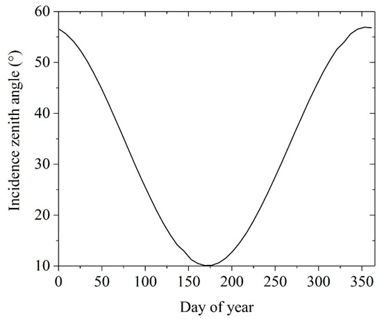
Figure 2.
Temporal variation of the incidence zenith angles for the MCD43A4 imageries over our study area in the study year (2017).
2.3. Retrieval Algorithm
The physically-based grassland AGB retrieval method was proposed to rely on the basic understanding that grassland is herbaceous, and therefore AGB can be represented as the product of leaf dry matter content (Cm) and leaf area index (LAI), i.e., AGB = Cm × LAI. Cm and LAI are vegetation parameters at leaf and canopy scales, respectively. Therefore, it is feasible to develop a physically-based grassland AGB retrieval method if a vegetation radiative transfer model contains the above two parameters.
Two main components are included in the proposed physically-based method: (1) radiative transfer model parameterization; and (2) radiative transfer model inversion. They will be introduced in detail in Section 2.3.1 and Section 2.3.2, respectively.
2.3.1. PROSAIL Model
From the perspective of model inversion, an appropriate model should be as realistic as possible to explain the variation of reflectance and, at the same time, as simple as possible to effectively solve the ill-posed inverse problem [33]. PROSAIL model was selected in this study, because it can achieve a proper comprise between reality and simplicity.
PROSAIL model is a combination of the SAILH canopy reflectance model [21] and the PROSPECT leaf optical properties model [20]. LAI and Cm are input parameters of the SAILH and PROSPECT model, respectively, and therefore can both be estimated.
SAILH simulates the canopy bi-directional reflectance in the range of 400 nm to 2500 nm as a function of input variables related to the structure of the canopy, the leaf optical properties (reflectance and transmittance), the background soil reflectance, fraction of diffuse incoming solar radiation and the sun-view geometry [21]. Canopy structure parameters include leaf area index (unitless), averaged leaf inclination angle (°), hot spot size (unitless). The leaf optical properties used for SAILH was simulated through the PROSPECT model [20]. The entire inputs include leaf chlorophyll content (mg·cm−2), leaf structure parameter (unitless), leaf equivalent water thickness (g·cm−2), leaf dry matter content (g·cm−2). The background reflectance spectrum can be simulated using the reflectance spectrum of fluvio-aquic soil multiplied by a brightness coefficient, which was used to depict changes induced by moisture and roughness in soil brightness [34,35]. Concerning the fraction of diffuse incoming solar radiation, a constant value across all wavelengths is often employed in many similar studies, as this parameter showed very limited influence on the simulated reflectance [18,34,36,37,38]. Finally, the sun-view geometry is described by the incidence zenith angle, view zenith angle, and the relative azimuth angle.
The parameterization of PROSAIL model is the prerequisite for our physically-based grassland AGB retrieval method. To improve the generality of the physically-based grassland AGB retrieval method, no field measurement data was used during the determination of the distribution of the canopy, leaf, and soil parameters. Rather, they were determined according to the literature regarding grassland parameters retrieval from PROSAIL model [23,34,37]. See Table 2 for the selected parameter intervals of main model parameters.
Table 2.
Distribution of the canopy, leaf, and soil parameters used in the PROSAIL parameterization. Parameters values are drawn randomly within these specific ranges.
2.3.2. The Lookup Table (LUT) Inversion
The lookup table (LUT) method is by nature the direct comparison of radiative transfer model simulated spectra against the observed spectra. It is a simple and widely-used inversion method in the field of vegetation parameter retrieval from remote sensing data [18]. LUT consists two main steps: LUT generation and LUT searching.
LUT generation: 100,000 parameter combinations were firstly randomly generated following uniform distributions. The ranges (minimum and maximum) for each of the 8 main model parameters are summarized in Table 2. The fraction of diffuse incoming solar radiation was set as 0, i.e., diffuse incoming solar radiation was ignored, given the fact that MCD43A4 is a bi-directional reflectance product. As for the sun-view geometry, the incidence zenith angle was set from 10° to 55° with a step of 5°. The dynamic range of the sun zenith angle was determined according to the its temporal variation for the MCD43A4 imageries over our study area simulated by the astronomical model [32]. (Figure 2). The view zenith angle and the relative azimuth angle were both set as 0°, to simulate the nadir-viewing condition. The incidence zenith angle range was determined by the annual variation of the local solar noon zenith angle in our study area (see Figure 2). Each parameter combination was then used to drive the PROSAIL model, and obtain simulated spectra covering wavelength from 400 nm to 2500 nm. As recommended by similar studies [18,39], a 5% Gaussian white noise was added to the simulated spectra to account for the remote sensing observation uncertainty. Finally, the continuous spectrums were converted into MODIS 1-7 channels reflectance values by means of the sensor relative spectral response (RSR).
LUT searching: To find the solution to the inverse problem for a given MCD43A4 pixel, the relative root mean squared error (R-RMSE) between measured and LUT-stored spectra is calculated as
where n (=7) is the number of spectral bands used, RiMCD is the MCD43A4 reflectance at band i, and RiLUT is the PROSAIL simulated reflectance stored in LUT. The relative RMSE rather than the absolute RMSE is used to account for the range discrepancy existed in the 7 MCD43A4 bands, e.g., the values for near infrared band is much larger than those for red band, and the red band will exert negligible influence if absolute RMSE is used. The solution corresponding the minimum RRMSE is not always the optimal solution because of the ill-posed nature of the inversion problem [38]. To alleviate this issue, we adopted the multi-solution method, i.e., the mean of the corresponding multiple target parameter values was provided as output estimate [18,34]
where t is the number of best matching spectra, LAIj and Cmj is the LAI and Cm corresponding the j-th best matching spectra. t was set as 50 based on literature [18,23,34,37] and our own tests and trials.
2.3.3. Assessment of Algorithm Performance
The assessment of the proposed physically-based grassland AGB retrieval method was conducted in the two following aspects:
Comparison with reference AGB map: The reference AGB map upscaled directly from the field measurements was seen as the proxy of ‘true values’ to assess the accuracy of the AGB map generated from the physically-based method. The reference AGB was aggregated to the same spatial resolution (500 m) as the MCD43A4 product before validation. We used the reference AGB map rather than the field measurements per se because there is obvious scale difference between sampling plots and MCD43A4 pixels (100 m vs. 500 m), and the spatial heterogeneity within the MCD43A4 pixel would cause scale error [40,41,42]. As recommended by the Committee Earth Observing Satellites’ Working Group on Calibration and Validation (CEOS WGCV), the ‘bottom-up’ validation approach through reference maps could significantly immediate the uncertainty caused by scale discrepancy, and provide more objective validation results [43]. A pixel-by-pixel comparison was conducted to calculate the RMSE and relative RMSE (RRMSE) between the reference and estimated AGB, as indicators representing the absolute and relative accuracy. The spatial distribution of the reference and estimated AGB maps was also compared to check whether the physically-based method can reproduce the spatial pattern of the ‘true’ case.
Temporal dynamic analysis: 46 AGB maps covering our study area in 2017 was generated. The temporal distribution of the AGB maps corresponds to that of our downloaded MCD43A4 (Section 2.2.2). The mean of each AGB map was calculated, and its temporal profile was analyzed to check that whether the estimated AGB time series can capture the grassland phenology. Moreover, the time series of estimated LAI and Cm, as elements to calculate AGB (see Equation (2)), was also analyzed.
3. Results
3.1. Comparison with Reference AGB Map
Figure 3 shows the direct pixel-by-pixel comparison between the reference and estimated AGB in DOY 225, 2017, corresponding to the field campaign (Section 2.2.1). Whilst, slight over-estimation and under-estimation can be found when reference AGB is less than 200 g·m−2 and between 300 and 350 g·m−2, respectively, a satisfactory accuracy is obtained from the proposed physically-based retrieval method with RMSE and R-RMSE of 60.06 g·m−2 and 18.1%, respectively.
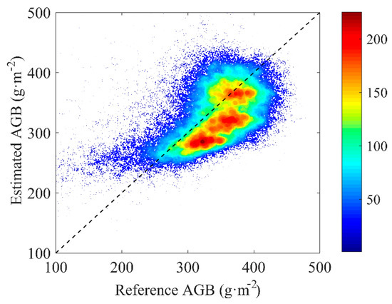
Figure 3.
Density scatterplots between the estimated and reference aboveground biomass (AGB) in DOY 225, 2017.
The estimated AGB map on DOY 225, 2017 (Figure 4) exhibits nearly identical spatial pattern as that of reference map (Figure 1b). For example, areas near rivers (bottom-left part) are characterized by high AGB because of easy access to moisture.
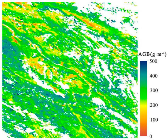
Figure 4.
Aboveground biomass (AGB) map (DOY 225, 2017) generated from the proposed method.
3.2. Temporal Dynamic
The temporal evolution of estimated AGB for our study area is shown in Figure 5. From a first analysis, the estimated AGB satisfactorily reproduces the seasonal variation and fits the mean value of the reference map very well. The growing season of the grassland spanned from ~ DOY 81 to 313. The growing peak appeared on ~ DOY 193, with value of 365.3 g·m−2. Note that the AGB in dormancy was not zero. This is because the grassland in our study area is divided into summer pastures and winter pastures by local people [30], and the winter pastures are adhered to much withered grass to feed the livestock during winter.
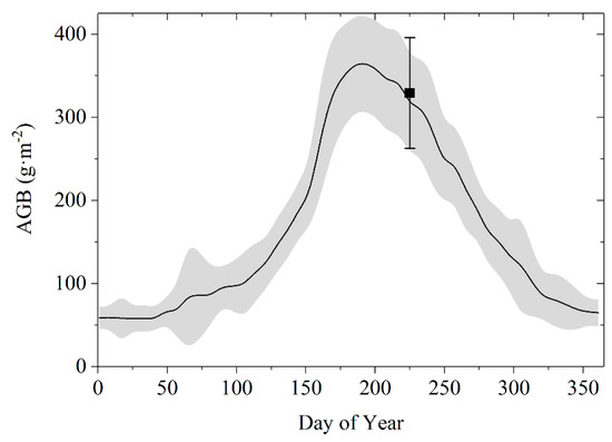
Figure 5.
Temporal profile of the estimated aboveground biomass (AGB) in our study area. The shaded area represents standard deviation of estimated AGB. The mean and standard deviation of the reference map are displayed as solid box and corresponding error bar.
The LAI and Cm used to calculate the AGB can also be retrieved simultaneously. Their temporal evolution was also analyzed (Figure 6). The LAI temporal profile is very similar with that of AGB. This is expected considering the fact that leaves are the only carrier for grassland AGB. A close inspection finds that Cm shows a contrary seasonal variation as that of LAI and AGB. This is because during the dormancy and senescence periods, grassland leaves contain low moisture due to the moisture stress. During the growing peak (DOY 193), the growing environment is favorable, resulting in the highest moisture content (lowest Cm) for leaves. The rational temporal profiles of LAI and Cm further confirm the rationality of the physically-based AGB retrieval method.
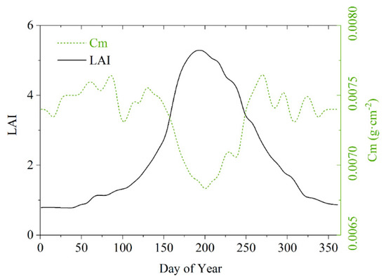
Figure 6.
Temporal profiles of the estimated leaf area index (LAI) and dry matter content (Cm) used to calculate the aboveground biomass (AGB).
4. Discussion
This study proposed a physically-based grassland retrieval method based on the inversion of PROSAIL model against MCD43A4 imagery. Validation showed that it could reproduce the reference AGB map, which generated by upscaling the field measurements, in terms of magnitude and spatial distribution. The estimated AGB time series also agreed reasonably well with the expected temporal dynamic trends of the grassland in our study area.
Empirically-based grassland AGB retrieval methods, relying on the regression relationship between field AGB measurements and vegetation indices, are relatively mature and widely represented in literature. For example, Xu et al. obtained an accuracy of 85.6% when MODIS GPP and NDVI products were used as depended variables [2]. He et al. found that when the MODIS LAI serving as dependent variables the corresponding RMSE was 54.25 g·m−2 [44]. The above two studies with field measurements involved in the calibration of the retrieval method attained only very slightly better results than our physically-based method without any field information involved (RMSE = 60.06 g·m−2, RRMSE = 18.1%). Our method even outperforms some empirical method in accuracy, e.g., Liang et al. reported a RMSE of 88.71 g·m−2 when empirical methods were used [11]. Many other studies confirm the conclusion that our physically-based method can achieve similar accuracy with empirical ones [5,9,10]. The most obvious advantage of the physical method over empirical ones does not lie in the accuracy, but in its generality [45]. Besides the time-consuming and labor-intensive nature, the empirical methods are also subject to the representativeness of the field measurement, and therefore, are time- and site-specific. However, our physically-based method is applicable for grassland nearly at anytime and anywhere, because PROSAIL model can simulate grassland reflectance in a wide range of scenarios [20,21]. In fact, it is the very reason that the proposed method can reproduce the expected temporal dynamic trends of the grassland (see Figure 5).
Direct comparison reveals that the estimated AGB is slightly over-estimated and under-estimated the reference vales when the reference vales are less than 200 g·m−2 and between 300 and 350 g·m−2, respectively. The over-estimation may be because of the unspecific parameterization of brightness coefficient which influences the retrieved results significantly when the AGB is small. This implies that the localization of the PROSAIL model would further improve the performance of our method. The under-estimation of our method for the medium AGB values may come from the neglect of non-herbaceous organs of grass, e.g., stem. The proportion of non-herbaceous organs decreases as the growth of the vegetation, and so the ‘big-leaf structures’ assumption of our method would not result in obvious under-estimation when the AGB is larger than 350 g·m−2. There is not only grass in the grassland, but also other species, so the estimated AGB will be over-estimated or under-estimated.
Traditional AGB validation procedures rely on the direct comparison between the retrieved values and field measurements. Two main drawbacks exist in the direct application of field measurements: First, the granularity difference between sampling plots and MDC43A4 pixels (100 m vs. 500 m) would induce scale error [40,41,43]. Second, the spatially sparse nature of the field measurements makes the spatial pattern comparison between estimated and reference values impossible. It is worth noting that the reference map per se is also with uncertainty. The quantification of the uncertainty involved in the upscaling procedure is challenging because of the lack of “true” map [46]. The choice of reference values (field measurements or upscaled map) for AGB validation depends on the tradeoff between uncertainties from scale difference and upscaling procedure. Coarse resolution pixels are often characterized by high degree of heterogeneity, resulting in obvious scale error during validation. This is also the reason why CEOS WGCV recommended using reference maps to validate coarse resolution remote sensing products [42]. Therefore, we argue that uncertainty from scale difference would outweigh that from upscaling procedure, and employed the reference map as benchmark to validate the estimated AGB.
It is worth noting that the estimated temporal evolution of Cm is shaky, especially in the dormancy and senescence periods (Figure 6). However, the realistic variation of Cm would not be so shaky. In fact, this fake variation is caused by the lack of information content of MODIS bands to estimate Cm. For example, Wang et al. [24] found that a narrow-band, normalized index combining two distinct wavebands centered at 1649 nm and 1722 nm was needed to estimate Cm, and Féret et al. found that reflectance at 1500 nm is also critical for estimating Cm [25]. Yet MODIS sensor cannot collect reflectance at the above three key bands (see Table 1). More advanced sensors with dedicated band configuration are needed to further improve Cm retrieval accuracy in future.
The greatest improvement of our method over other physically-based methods is that our method is fully physical, i.e., no empirical variable or relationship is needed. Existing physically-based methods are also needed to support the field measurements. For example, Punalekar et al. [22] transformed estimated LAI to AGB through a constant Cm which is estimated through the regression of field measured LAI and AGB. Quan et al. [23] parameterize the PROSAIL model based on an empirical relationship between leaf equivalent water thickness and Cm. However, the ratio between them is temporally variational, which is the main driver causing the temporal variation of Cm (see Figure 6). Therefore, field measurements are also the prerequisite in Punalekar’s [22] and Quan’s [23] method for calibration. Conversely, the fully physical nature of our method makes it feasible for other grassland areas. Besides the calibration procedure, the data sources are also different between our method and other physically-based methods: MODIS was employed rather than Landsat or Sentinel data as in [22,23], respectively. We selected MODIS because of two following reasons: (1) it has a high revisiting frequency, making the spatiotemporally continuous AGB monitoring possible after the temporal compositing; (2) the incidence angle of the MCD43A4 product has been normalized to local solar noon of the day [31], and therefore the range of sun-view geometries is limited, reducing the size of the LUT.
The temporal variation of Cm is very limited, ranging from 0.0065 to 0.0075 g·cm−2 (see Figure 6). This is inconsistent with many other foliar scale studies, which finds that the variation in Cm of leaves can cover obviously wider range [47]. This inconsistence may come from the scale difference (foliar vs. canopy). The canopy consists of many leaves and even different species, the difference of leaves in Cm may be smoothed, resulting in a relative constant Cm. The relatively constant Cm at canopy scale was also reported by Punalekar et al. [22]. In fact, the canopy scale constant Cm assumption is the basis of their method. The two main advantages of our method are due to its fully physical nature: (1) the small temporal variation of Cm was accounted for; (2) the Cm can be estimated from remote sensing data without the support of field measurement.
Further improvements of our method include: (1) The soil reflectance can be replaced by more representative spectral libraries, especially those dedicatedly collected for grassland soil [48]. (2) More advanced models are worth testing to further improve the representativeness of the LUT. For example, Qiu et al. [49] developed the PROSPECT-g model which has higher accuracy in Cm estimation. (3) The application of the proposed method for other herbaceous plants, e.g., crop, is also worth testing.
5. Conclusions
This study proposed a physically-based grassland aboveground biomass (AGB) retrieval method which relies on the basic understanding that grassland is herbaceous, and therefore AGB can be represented as the product of leaf dry matter content (Cm) and leaf area index (LAI), i.e., AGB = Cm × LAI. The lookup table (LUT) inversion of PROSAIL model against MCD43A4 imagery was used to estimate Cm and LAI and finally converted to AGB. The proposed method was validated in the Zoige Plateau, China. Results show that it could reproduce the reference AGB map, which is generated by upscaling the field measurements, in terms of magnitude (with RMSE and R-RMSE of 60.06 g·m−2 and 18.1%, respectively) and spatial distribution. The estimated AGB time series also agreed reasonably well with the expected temporal dynamic trends of the grassland in our study area. Our study paved new way to monitor grassland AGB dynamics at regional and larger scales without the support of field measurement.
Author Contributions
Conceptualization, A.L. and G.Y.; Methodology, G.Y.; Writing—original draft preparation, L.H.; Writing—review and editing, G.Y.; Visualization, X.N.; Field measurement implementation, J.B.
Funding
This research was funded by National Natural Science Foundation of China (no. 41631180 and no. 41571373), the Strategic Priority Research Program of the Chinese Academy of Sciences (XDA19030303), the National Key Research and Development Program of China (no. 2016YFA0600103 and 2016YFC0500201-06), and the 135 Strategic Program of the Institute of Mountain Hazards and Environment, CAS (SDS-135-1708).
Acknowledgments
The authors are very thankful for Land Processes Distributed Active Archive Center (LPDAAC) for the free access to MCD43A4 product. We also acknowledge Prof Wout Verhoef’s team for sharing the PROSAIL model code.
Conflicts of Interest
The authors declare no conflict of interest.
References
- Dusseux, P.; Hubert-Moy, L.; Corpetti, T.; Vertès, F. Evaluation of SPOT imagery for the estimation of grassland biomass. Int. J. Appl. Earth Obs. Geoinf. 2015, 38, 72–77. [Google Scholar] [CrossRef]
- Fu, X.; Tang, C.; Zhang, X.; Fu, J.; Jiang, D. An improved indicator of simulated grassland production based on MODIS NDVI and GPP data: A case study in the Sichuan province, China. Ecol. Indic. 2014, 40, 102–108. [Google Scholar] [CrossRef]
- Kumar, L.; Mutanga, O. Remote sensing of above-ground biomass. Remote Sens. 2017, 9, 935. [Google Scholar] [CrossRef]
- Piao, S.; Fang, J.; Zhou, L.; Tan, K.; Tao, S. Changes in biomass carbon stocks in China’s grasslands between 1982 and 1999. Glob. Biogeochem. Cycles 2007, 21. [Google Scholar] [CrossRef]
- Jia, W.; Liu, M.; Yang, Y.; He, H.; Zhu, X.; Yang, F.; Yin, C.; Xiang, W. Estimation and uncertainty analyses of grassland biomass in Northern China: Comparison of multiple remote sensing data sources and modeling approaches. Ecol. Indic. 2016, 60, 1031–1040. [Google Scholar] [CrossRef]
- Yin, G.; Li, A.; Wu, C.; Wang, J.; Xie, Q.; Zhang, Z.; Nan, X.; Jin, H.; Bian, J.; Lei, G. Seamless upscaling of the field-measured grassland aboveground biomass based on gaussian process regression and gap-filled landsat 8 OLI reflectance. Int. J. Geo–Inf. 2018, 7, 242. [Google Scholar] [CrossRef]
- Shoko, C.; Mutanga, O.; Dube, T. Progress in the remote sensing of C3 and C4 grass species aboveground biomass over time and space. ISPRS J. Photogramm. 2016, 120, 13–24. [Google Scholar] [CrossRef]
- Gao, T.; Yang, X.; Jin, Y.; Ma, H.; Li, J.; Yu, H.; Yu, Q.; Zheng, X.; Xu, B. Spatio-temporal variation in vegetation biomass and its relationships with climate factors in the Xilingol grasslands, Northern China. PLoS ONE 2013, 8, e83824. [Google Scholar] [CrossRef]
- Jin, Y.; Yang, X.; Qiu, J.; Li, J.; Gao, T.; Wu, Q.; Zhao, F.; Ma, H.; Yu, H.; Xu, B. Remote sensing-based biomass estimation and its spatio-temporal variations in temperate grassland, Northern China. Remote Sens. 2014, 6, 1496–1513. [Google Scholar] [CrossRef]
- Li, F.; Zeng, Y.; Luo, J.; Ma, R.; Wu, B. Modeling grassland aboveground biomass using a pure vegetation index. Ecol. Indic. 2016, 62, 279–288. [Google Scholar] [CrossRef]
- Liang, T.; Yang, S.; Feng, Q.; Liu, B.; Zhang, R.; Huang, X.; Xie, H. Multi-factor modeling of above-ground biomass in alpine grassland: A case study in the Three-River Headwaters Region, China. Remote Sens. Environ. 2016, 186, 164–172. [Google Scholar] [CrossRef]
- Duursma, R.A.; Marshall, J.D.; Robinson, A.P. Leaf area index inferred from solar beam transmission in mixed conifer forests on complex terrain. Agric. For. Meteorol. 2003, 118, 221–236. [Google Scholar] [CrossRef]
- Zhang, B.; Zhang, L.; Xie, D.; Yin, X.; Liu, C.; Liu, G. Application of synthetic NDVI time series blended from landsat and MODIS data for grassland biomass estimation. Remote Sens. 2016, 8, 10. [Google Scholar] [CrossRef]
- Xie, Y.; Sha, Z.; Yu, M.; Bai, Y.; Zhang, L. A comparison of two models with Landsat data for estimating above ground grassland biomass in Inner Mongolia, China. Ecol. Model. 2009, 220, 1810–1818. [Google Scholar] [CrossRef]
- Widlowski, J.L.; Pinty, B.; Lopatka, M.; Atzberger, C.; Buzica, D.; Chelle, M.; Disney, M.; Gastellu-Etchegorry, J.P.; Gerboles, M.; Gobron, N.; et al. The fourth radiation transfer model intercomparison (RAMI-IV): Proficiency testing of canopy reflectance models with ISO-13528. J. Geophys. Res. Atmos. 2013, 118, 6869–6890. [Google Scholar] [CrossRef]
- Yin, G.F.; Li, A.N.; Zhao, W.; Jin, H.A.; Bian, J.H.; Wu, S.B.A. Modeling canopy reflectance over sloping terrain based on path length correction. IEEE Trans. Geosci. Remote Sens. 2017, 55, 4597–4609. [Google Scholar] [CrossRef]
- Zeng, Y.; Li, J.; Liu, Q.; Huete, A.R.; Yin, G.; Xu, B.; Fan, W.; Zhao, J.; Yan, K.; Mu, X. A radiative transfer model for heterogeneous agro-forestry scenarios. IEEE Trans. Geosci. Remote Sens. 2016, 54, 4613–4628. [Google Scholar] [CrossRef]
- Verrelst, J.; Rivera, J.P.; Leonenko, G.; Alonso, L.; Moreno, J. Optimizing LUT-based RTM inversion for semiautomatic mapping of crop biophysical parameters from sentinel-2 and-3 data: Role of cost functions. IEEE Trans. Geosci. Remote Sens. 2014, 52, 257–269. [Google Scholar] [CrossRef]
- Baret, F.; Weiss, M.; Lacaze, R.; Camacho, F.; Makhmara, H.; Pacholcyzk, P.; Smets, B. GEOV1: LAI and FAPAR essential climate variables and FCOVER global time series capitalizing over existing products. Part1: Principles of development and production. Remote Sens. Environ. 2013, 137, 299–309. [Google Scholar] [CrossRef]
- Jacquemoud, S.; Verhoef, W.; Baret, F.; Bacour, C.; Zarco-Tejada, P.J.; Asner, G.P.; Francois, C.; Ustin, S.L. PROSPECT plus SAIL models: A review of use for vegetation characterization. Remote Sens. Environ. 2009, 113, S56–S66. [Google Scholar] [CrossRef]
- Verhoef, W. Light scattering by leaf layers with application to canopy reflectance modeling: The SAIL model. Remote Sens. Environ. 1984, 16, 125–141. [Google Scholar] [CrossRef]
- Punalekar, S.M.; Verhoef, A.; Quaife, T.L.; Humphries, D.; Bermingham, L.; Reynolds, C.K. Application of Sentinel-2A data for pasture biomass monitoring using a physically based radiative transfer model. Remote Sens. Environ. 2018, 218, 207–220. [Google Scholar] [CrossRef]
- Quan, X.; He, B.; Yebra, M.; Yin, C.; Liao, Z.; Zhang, X.; Li, X. A radiative transfer model-based method for the estimation of grassland aboveground biomass. Int. J. Appl. Earth Obs. Geoinf. 2017, 54, 159–168. [Google Scholar] [CrossRef]
- Wang, L.; Hunt, E.R., Jr.; Qu, J.J.; Hao, X.; Daughtry, C.S. Towards estimation of canopy foliar biomass with spectral reflectance measurements. Remote Sens. Environ. 2011, 115, 836–840. [Google Scholar] [CrossRef]
- Féret, J.-B.; le Maire, G.; Jay, S.; Berveiller, D.; Bendoula, R.; Hmimina, G.; Cheraiet, A.; Oliveira, J.; Ponzoni, F.; Solanki, T.; et al. Estimating leaf mass per area and equivalent water thickness based on leaf optical properties: Potential and limitations of physical modeling and machine learning. Remote Sens. Environ. 2018, 217, 110959. [Google Scholar] [CrossRef]
- Ullah, S.; Si, Y.; Schlerf, M.; Skidmore, A.K.; Shafique, M.; Iqbal, I.A. Estimation of grassland biomass and nitrogen using MERIS data. Int. J. Appl. Earth Obs. Geoinf. 2012, 19, 196–204. [Google Scholar] [CrossRef]
- Sibanda, M.; Mutanga, O.; Rouget, M. Examining the potential of Sentinel-2 MSI spectral resolution in quantifying above ground biomass across different fertilizer treatments. Isprs J. Photogramm. 2015, 110, 55–65. [Google Scholar] [CrossRef]
- Liu, S.; Cheng, F.; Dong, S.; Zhao, H.; Hou, X.; Wu, X. Spatiotemporal dynamics of grassland aboveground biomass on the Qinghai-Tibet Plateau based on validated MODIS NDVI. Sci. Rep. 2017, 7, 4182. [Google Scholar] [CrossRef]
- Yang, Y.H.; Fang, J.Y.; Pan, Y.D.; Ji, C.J. Aboveground biomass in Tibetan grasslands. J. Arid Environ. 2009, 73, 91–95. [Google Scholar] [CrossRef]
- Wang, J.; Li, A.; Bian, J. Simulation of the grazing effects on grassland aboveground net primary production using DNDC model combined with time-series remote sensing data—a case study in Zoige Plateau, China. Remote Sens. 2016, 8, 168. [Google Scholar] [CrossRef]
- Schaaf, C.B.; Gao, F.; Strahler, A.H.; Lucht, W.; Li, X.W.; Tsang, T.; Strugnell, N.C.; Zhang, X.Y.; Jin, Y.F.; Muller, J.P.; et al. First operational BRDF, albedo nadir reflectance products from MODIS. Remote Sens. Environ. 2002, 83, 135–148. [Google Scholar] [CrossRef]
- Blanco-Muriel, M.; Alarcon-Padilla, D.C.; Lopez-Moratalla, T.; Lara-Coira, M. Computing the solar vector. Sol. Energy 2001, 70, 431–441. [Google Scholar] [CrossRef]
- Yin, G.F.; Li, J.; Liu, Q.H.; Fan, W.L.; Xu, B.D.; Zeng, Y.L.; Zhao, J. Regional leaf area index retrieval based on remote sensing: the role of radiative transfer model selection. Remote Sens. 2015, 7, 4604–4625. [Google Scholar] [CrossRef]
- Darvishzadeh, R.; Skidmore, A.; Schlerf, M.; Atzberger, C. Inversion of a radiative transfer model for estimating vegetation LAI and chlorophyll in a heterogeneous grassland. Remote Sens. Environ. 2008, 112, 2592–2604. [Google Scholar] [CrossRef]
- Xu, M.; Liu, R.; Chen, J.M.; Liu, Y.; Shang, R.; Ju, W.; Wu, C.; Huang, W. Retrieving leaf chlorophyll content using a matrix-based vegetation index combination approach. Remote Sens. Environ. 2019, 224, 60–73. [Google Scholar] [CrossRef]
- Campos-Taberner, M.; García-Haro, F.J.; Camps-Valls, G.; Grau-Muedra, G.; Nutini, F.; Crema, A.; Boschetti, M. Multitemporal and multiresolution leaf area index retrieval for operational local rice crop monitoring. Remote Sens. Environ. 2016, 187, 102–118. [Google Scholar] [CrossRef]
- Pasolli, L.; Asam, S.; Castelli, M.; Bruzzone, L.; Wohlfahrt, G.; Zebisch, M.; Notarnicola, C. Retrieval of leaf area index in mountain grasslands in the Alps from MODIS satellite imagery. Remote Sens. Environ. 2015, 165, 159–174. [Google Scholar] [CrossRef]
- Verger, A.; Baret, F.; Camacho, F. Optimal modalities for radiative transfer-neural network estimation of canopy biophysical characteristics: Evaluation over an agricultural area with CHRIS/PROBA observations. Remote Sens. Environ. 2011, 115, 415–426. [Google Scholar] [CrossRef]
- Combal, B.; Baret, F.; Weiss, M.; Trubuil, A.; Mace, D.; Pragnere, A.; Myneni, R.; Knyazikhin, Y.; Wang, L. Retrieval of canopy biophysical variables from bidirectional reflectance—Using prior information to solve the ill-posed inverse problem. Remote Sens. Environ. 2003, 84, 1–15. [Google Scholar] [CrossRef]
- Garrigues, S.; Allard, D.; Baret, F.; Weiss, M. Influence of landscape spatial heterogeneity on the non-linear estimation of leaf area index from moderate spatial resolution remote sensing data. Remote Sens. Environ. 2006, 105, 286–298. [Google Scholar] [CrossRef]
- Yin, G.F.; Li, A.N.; Verger, A. Spatiotemporally representative and cost-efficient sampling design for validation activities in Wanglang experimental site. Remote Sens. 2017, 9, 1217. [Google Scholar] [CrossRef]
- Yin, G.F.; Li, J.; Liu, Q.H.; Li, L.H.; Zeng, Y.L.; Xu, B.D.; Yang, L.; Zhao, J. Improving leaf area index retrieval over heterogeneous surface by integrating textural and contextual information: A case study in the Heihe River Basin. IEEE Geosci. Remote Sens. Lett. 2015, 12, 359–363. [Google Scholar] [CrossRef]
- Morisette, J.T.; Baret, F.; Privette, J.L.; Myneni, R.B.; Nickeson, J.E.; Garrigues, S.; Shabanov, N.V.; Weiss, M.; Fernandes, R.A.; Leblanc, S.G.; et al. Validation of global moderate-resolution LAI products: A framework proposed within the CEOS Land Product Validation subgroup. IEEE Trans. Geosci. Remote Sens. 2006, 44, 1804–1817. [Google Scholar] [CrossRef]
- He, B.; Li, X.; Quan, X.; Qiu, S. Estimating the aboveground dry biomass of grass by assimilation of retrieved LAI into a crop growth model. IEEE J. Sel. Top. App. Ear. Obsev. Remote Sens. 2015, 8, 550–561. [Google Scholar] [CrossRef]
- Verrelst, J.; Camps-Valls, G.; Muñoz-Marí, J.; Rivera, J.P.; Veroustraete, F.; Clevers, J.G.P.W.; Moreno, J. Optical remote sensing and the retrieval of terrestrial vegetation bio-geophysical properties—A review. ISPRS J. Photogramm. Remote Sens. 2015, 108, 273–290. [Google Scholar] [CrossRef]
- Cohen, W.B.; Maiersperger, T.K.; Gower, S.T.; Turner, D.P. An improved strategy for regression of biophysical variables and Landsat ETM+ data. Remote Sens. Environ. 2003, 84, 561–571. [Google Scholar] [CrossRef]
- Ali, A.M.; Darvishzadeh, R.; Skidmore, A.K. Retrieval of specific leaf area from landsat-8 surface reflectance data using statistical and physical models. IEEE J. Sel. Top. Appl. Earth Obs. Remote Sens. 2017, 1–8. [Google Scholar] [CrossRef]
- Baldridge, A.M.; Hook, S.; Grove, C.; Rivera, G. The ASTER spectral library version 2.0. Remote Sens. Environ. 2009, 113, 711–715. [Google Scholar] [CrossRef]
- Qiu, F.; Chen, J.M.; Ju, W.; Wang, J.; Zhang, Q.; Fang, M. Improving the PROSPECT model to consider anisotropic scattering of leaf internal materials and its use for retrieving leaf biomass in fresh leaves. IEEE Trans. Geosci. Remote Sens. 2018, 56, 3119–3136. [Google Scholar] [CrossRef]
© 2019 by the authors. Licensee MDPI, Basel, Switzerland. This article is an open access article distributed under the terms and conditions of the Creative Commons Attribution (CC BY) license (http://creativecommons.org/licenses/by/4.0/).