Review

Monitoring Green Infrastructure for Natural Water Retention Using Copernicus Global Land Products

by
Andrea Taramelli
1,2,
Michele Lissoni
1,
Laura Piedelobo
3,*,
Emma Schiavon
1,
Emiliana Valentini
2,
Alessandra Nguyen Xuan
2 and
Diego González-Aguilera
3
1
Istituto Universitario di Studi Superiori di Pavia (IUSS), Palazzo del Broletto, Piazza della Vittoria 15, 27100 Pavia, Italy
2
Institute for Environmental Protection and Research (ISPRA), via Vitaliano Brancati 48, 00144 Roma, Italy
3
Department of Cartographic and Land Engineering, University of Salamanca, Hornos Caleros 50, 05003 Ávila, Spain
*
Author to whom correspondence should be addressed.
Remote Sens. 2019, 11(13), 1583; https://doi.org/10.3390/rs11131583
Submission received: 29 May 2019 / Revised: 17 June 2019 / Accepted: 28 June 2019 / Published: 3 July 2019

Abstract

:
Nature-based solutions are increasingly relevant tools for spatial and environmental planning, climate change adaptation (CCA), and disaster risk reduction (DRR). For this reason, a wide range of institutions, governments, and financial bodies are currently promoting the use of green infrastructure (GI) as an alternative or a complement to traditional grey infrastructure. A considerable amount of research already certifies the benefits and multi-functionality of GI: natural water retention measures (NWRMs), as GIs related specifically to the water sector are also known, are, for instance, a key instrument for the prevention and mitigation of extreme phenomena, such as floods and droughts. However, there are persisting difficulties in locating and identifying GI and one of the most promising solutions to this issue, the use of satellite-based data products, is hampered by a lack of well-grounded knowledge, experiences, and tools. To bridge this gap, we performed a review of the Copernicus Global Land Service (CGLS) products, which consist of freely-available bio-geophysical indices covering the globe at mid-to-low spatial resolutions. Specifically, we focused on vegetation and energy indices, examining previous research works that made use of them and evaluating their current quality, aiming to define their potential for studying GI and especially NWRMs related to agriculture, forest, and hydro-morphology. NWRM benefits are also considered in the analysis, namely: (i) NWRM biophysical impacts (BPs), (ii) ecosystem services delivered by NWRMs (ESs), and (iii) policy objectives (POs) expressed by European Directives that NWRMs can help to achieve. The results of this study are meant to assist GI users in employing CGLS products and ease their decision-making process. Based on previous research experiences and the quality of the currently available versions, this analysis provides useful tools to identify which indices can be used to study several types of NWRMs, assess their benefits, and prioritize the most suitable ones.

Graphical Abstract

1. Introduction

Green infrastructures (GIs) are often presented as nature-based solutions in the context of both spatial and environmental planning [1,2]. However, the concept can be applied to a greater variety of environments and remains extremely broad [3,4], to the point that, despite the increasing relevance of GIs in several policy areas, no universally-accepted definition exists [5,6,7,8]. In 2013, the European Union (EU) defined GI as “a strategically planned network of natural and semi-natural areas with other environmental features designed and managed to deliver a wide range of ecosystem services […]” [9].
This definition states that GIs are primarily spatial tools for the delivery of both green and blue (when considering aquatic systems) ecosystem services (ESs) in terrestrial, coastal, or marine areas [2,3,4,9,10,11]. ESs are classified either as (i) provisioning services, supplying natural resources; (ii) regulatory and maintenance; or (iii) cultural [12].
Multi-functionality is perhaps the most important characteristic of GIs, which are capable of delivering multiple benefits to both nature and human-beings [10,13]: Given their cost-effectiveness [14], it is advocated that, where possible, they should be preferred to single-purpose grey infrastructures. The restoration of a floodplain, a typical GI, is an example of this: Such a measure would provide flood risk reduction, water storage, biodiversity protection, and recreational opportunities [15], whereas only the first benefit would be delivered by grey flood defenses.
Over the past decade, GI’s potential as a policy tool to promote the establishment of a resilient society and a sustainable economic development has been increasingly acknowledged by policymakers [10,12,13]. In 2011, the EU Biodiversity Strategy to 2020 [16] explicitly stated the importance of incorporating GIs into spatial planning in order to achieve its target two, the maintenance and enhancement of ESs and the recovery of at least 15% of the degraded ecosystems across Europe.
Then, in 2013, the European Commission formulated a specific GI strategy, aiming to promote their uptake among stakeholders, encouraging investments, and developing trans-European GI networks [9]. The strategy outlined the need to incorporate GIs into key policies, recognizing it as an important tool to achieve a variety of policy objectives. For instance, GI can be employed to:
  • Store carbon, reduce greenhouse gas emissions, and lower the carbon footprint due to residential, transport and energy production sectors, as well as alleviate extreme weather events and natural disasters, thus supporting the EU Strategy on Adaptation to Climate Change [17].
  • Improve the connectivity between Natura 2000 core areas, established by the Habitats [18] and Birds Directives [19] and enhanced by the 2020 Biodiversity Strategy [16], and integrate them with the surrounding environment.
  • Avoid forest erosion, soil contamination, and the fragmentation and degradation of ecosystems, as required by the EU Forests Strategy [20].
  • Achieve several objectives of the Common Agricultural Policy (CAP) [21] and encourage agricultural sustainable practices.
  • Improve water quality and storage, treat waste water, reduce hydro-morphological pressures on river basins, and mitigate the impacts of floods and droughts, thus contributing to the goals of all EU water-related policies, including the Water Framework Directive [22], the Groundwater Directive [23], and the Floods Directive [24].
GIs related to the water sector are identified by the European Commission Directorate-General Department for Environment Policies (DG-ENV) as natural water retention measures (NWRMs). NWRMs are defined as “multi-functional measures that specifically aim to protect and manage water resources and address water-related challenges by restoring or maintaining ecosystems as well as natural features and characteristics of water bodies using natural means and processes […]” [25]. Thus, their main function is to act upon water-dependent ecosystems to enhance the natural characteristics that enable them to retain water. This makes it possible to minimize runoff peaks during periods of abundant precipitation as well as to store water to cope with dry periods, increasing the resilience of the water ecosystem against extreme events, such as floods and droughts [17,26,27,28].
In 2013, the DG-ENV launched a two-year-long NWRM initiative [29], with the aim of developing a knowledge base and bringing together all parties interested in NWRM design and implementation. The initiative produced a catalogue of 53 NWRMs, classified per sector: Agriculture, forest, hydro-morphology, and urban. It also studied NWRM benefits, formulating a list of 17 NWRM biophysical impacts (BPs) resulting from water retention, 14 ecosystem services (ESs) delivered by NWRMs, and 14 EU policy objectives (POs) that NWRMs can help to reach.
In this work, we dealt with GIs, and specifically with NWRMs, by considering first the needs of users and stakeholders related to the implementation, monitoring, control, and management of actual or potential GIs. We then attempted to fulfil these needs by proposing solutions based on remotely-sensed data within the Copernicus regulation [30]. Such data, especially when freely available, up-to-date and in near-real-time, shows great potential, considering the constant changes undergone by Earth’s ecosystems due to natural land and atmospheric conditions and under the pressure of human activities [31,32,33]. Its applications include the parametrization of a wide variety of ecosystem models, the reproduction of ecosystem dynamics, and the estimation of natural risks to ecosystems or future scenarios, which can improve the formulation of environmental and conservation policies [34,35,36].
In order to monitor and manage ecosystem changes, scientists have developed, in the framework of remote sensing applications, highly useful indices and approaches for evaluating both qualitatively and quantitatively the vegetative-water-energy nexus of natural surfaces through the execution of spectral measurements [33,34,36,37,38,39]. The worldwide known Copernicus Global Land Service (CGLS) [40], a component of the Land Monitoring Core Service of the Copernicus Earth Observation program, provides in particular a freely-available set of products based on qualified bio-geophysical indices. These products are arranged into long-term time series and monitor the status and evolution of the land surface on a global scale at mid-to-low spatial resolutions (300 m and 1 km) and in near-real-time. They can be used to monitor components and processes of the Earth system, including the vegetation, water cycle, energy budget, and terrestrial cryosphere.
Our study aimed to develop tools for users and stakeholders to ascertain the potential of CGLS products for the identification, monitoring, and assessment of GIs. As we were particularly interested in GIs for the reduction and mitigation of water-related hazards, such as floods and droughts, the analysis focused on determining the most suitable indices for the monitoring of NWRMs. Therefore, we performed a review of previous research experiences that employed the bio-geophysical indices provided in the CGLS vegetation and energy products and then used the review’s results to assess whether each product could potentially be used to monitor several types of NWRMs and their benefits, also taking into account the quality of the products’ currently-available versions.
Ultimately, the purpose of this review was building an evidence base that, merged with future research and developments, would allow us to understand the requirements to properly monitor and identify NWRM and their benefits using operational information data streams covered by current (or planned) Copernicus capacity. Performing this kind of analysis is essential to provide well-grounded advice for the future inclusion of new products and services inside the Copernicus framework to suitably cover institutional and private business processes and needs. Thus, products under demonstration, pre-operational, or operational conditions could benefit from these analyses, having a clear view of their current and potential use.
The present article is organized as follows: After describing in detail CGLS products and GI/NWRM characteristics, benefits, and regulating policies, the methodology section outlines the input data used for our review of the scientific literature, the results of which are expressed through the use of Sankey diagrams and flowcharts. The results section indicates which vegetation and energy indices, among those provided by the CGLS products, are potentially most useful for the monitoring of each NWRM, biophysical impact, ecosystem service, and policy objective. Moreover, this section indicates the quality that can be expected when using the CGLS bio-geophysical indices in terms of their continuity along the globe, spatial and temporal consistencies, and overall accuracy. The discussion section debates the results derived from the analysis and provides guidelines for users in the form of flow diagrams showing the most recommended products. Finally, all the conclusions derived from the study are summarized.

2. Materials and Methods
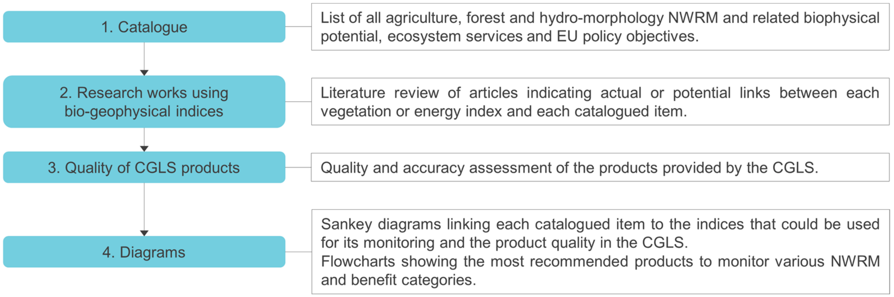
Our approach, shown in Figure 1, entailed firstly considering the review of previous scientific works that used or evidenced the potential use, either direct or indirect, of one of the bio-geophysical indices provided by the Copernicus Global Land Service (CGLS) vegetation or energy products to monitor a natural water retention measure (NWRM), observe a NWRM biophysical impact (BP), certify the delivery of a NWRM ecosystem service (ES), or verify the achievement of a NWRM-related policy objective (PO) from the targets of EU directives. We also focused on the actual quality that users could expect using the last-updated versions of the CGLS products in terms of the data continuity along the globe, spatial and temporal consistencies, and accuracy when compared with other satellite-based products [40]. Finally, the outcomes were combined in Sankey diagrams and flowcharts designed for the benefit of GI users.

2.1. Catalogue

The first step of our approach was organizing a catalogue of the relevant NWRMs, BPs, ESs, and POs (Table 1). We made use of the catalogues developed by the DG-ENV NWRM initiative [29].
The original catalogue of NWRMs contained 53 measures divided in four sectors: (i) Agriculture, (ii) forest, (iii) hydro-morphology, and (iv) urban. As the present analysis was involved in a research [41] specifically tackling rural GI development, its monitoring, and the management of water-related natural hazards, the review only studied the 41 NWRMs included in the first three categories (Table 1).
The catalogue of the biophysical impacts resulting from water retention was left unaltered: All 17 BPs, originally divided into either direct (i.e., runoff control) or indirect (i.e., pollution reduction, soil conservation, habitat creation, or climate alteration), were considered. On the other hand, the list of NWRM-related ecosystem services was significantly altered: Originally containing 14 ESs, classified as (i) provisioning, (ii) regulatory and maintenance, (iii) cultural, or (iv) abiotic services, this catalogue was reduced to the 9 ESs belonging to the first two categories, while the other two were excluded as none of the cultural (i.e., recreational opportunities) or abiotic services (i.e., navigation or energy production) were actually relevant for the final goal of monitoring and assessing GIs in rural environments for the reduction and mitigation of water-related natural hazards (Table 2).
The list of EU policy objectives, finally, originally contained a list of 14 NWRM-related POs expressed by the Water Framework Directive (WFD) [22], the Floods Directive (FD) [24], the Habitats and Birds Directives (HD and BD) [18,19], and the 2020 Biodiversity Strategy (BS) [16]. This list was left mostly unaltered, with the sole exception of PO11, which is explicitly linked to GI deployment and was henceforth considered redundant, considering the method used to perform the literature review, further explained in Section 2.2.2 (Table 2).

2.2. Research Works Using Bio-Geophysical Indices

2.2.1. CGLS Vegetation and Energy Products

Nowadays, aerial and satellite remote sensing techniques are the foremost source of spatial information due to their capability to catch large areas and monitor bio-geophysical parameters with competitive spatial and temporal resolutions [42,43]. The bio-geophysical indices freely offered by the Copernicus Global Land Service through its vegetation and energy products can be applied to a wide range of thematic areas, such as global crop monitoring and food security; forest, water, and natural resources management; land carbon modelling; or weather and climate forecasting [40]. The indices have been validated using other existing global products derived from remotely-sensed data, mostly produced by the MODIS (Moderate-resolution Imaging Spectrometer) sensor platform [44]. Moreover, accuracy assessments have been performed through the comparison with ground-based reference data, especially from the 2012 Land Use and Cover Area frame Survey (LUCAS) [45].
Focusing on CGLS vegetation products (as of November 2018), the widely-used normalized difference vegetation index (NDVI) gives an indication of the current greenness of the natural surface [33,36]. Derived from this index are the VCI and VPI (vegetation condition and productivity indices; the latter has now been discontinued), which compare measured NDVI values respectively to its long-term average and to its historical maximum and minimum. Other products provide measurements of physical variables of the canopy: The leaf area index (LAI), the fraction of vegetation cover (FCOVER), and the fraction of radiation absorbed for the photosynthesis (FAPAR) quantify the density, extent, and health of the vegetation, respectively. On the other hand, dry matter productivity (DMP) and gross dry matter productivity (GDMP) feature the growth of standing biomass and have specific agronomic applications. The soil water index (SWI) adds complexity to the analysis by quantifying the moisture condition at various soil depths. Finally, the maps of burned areas delineate the zones of the globe that have been affected by fire events [34,46,47,48,49,50,51,52,53,54,55,56,57,58,59,60,61,62,63,64,65]. The Global Climate Observing System (GCOS) recognizes the maps of burned areas, FAPAR, LAI, and SWI as essential climate variables (ECVs) [40].
The energy bio-geophysical variables, on the other hand, assess the energy budget at the land surface. Top-of-canopy reflectance (TOCR) and surface albedo quantify the part of the sunlight reflected by the surface, respectively, dependent and independent from the angular observation conditions (the first has been discontinued). In addition, the land surface temperature (LST) indicates how hot or cold the ground is and depends on the surface albedo, vegetation cover, and soil moisture [66,67,68,69].
These bio-geophysical indices are useful for weather and climate forecasting as they are the resulting effect of key forcing variables controlling the energy exchanges between the continental surface and the atmosphere. Since they also detect how energy is distributed between the ground and vegetation, they have become essential for crop growth modelling. As a sensitive indicator of environmental vulnerability, surface albedo is especially efficient for the detection of land degradation and desertification [66,67,68,69]. Table 3 shows the CGLS products considered in the literature review together with their main characteristics.

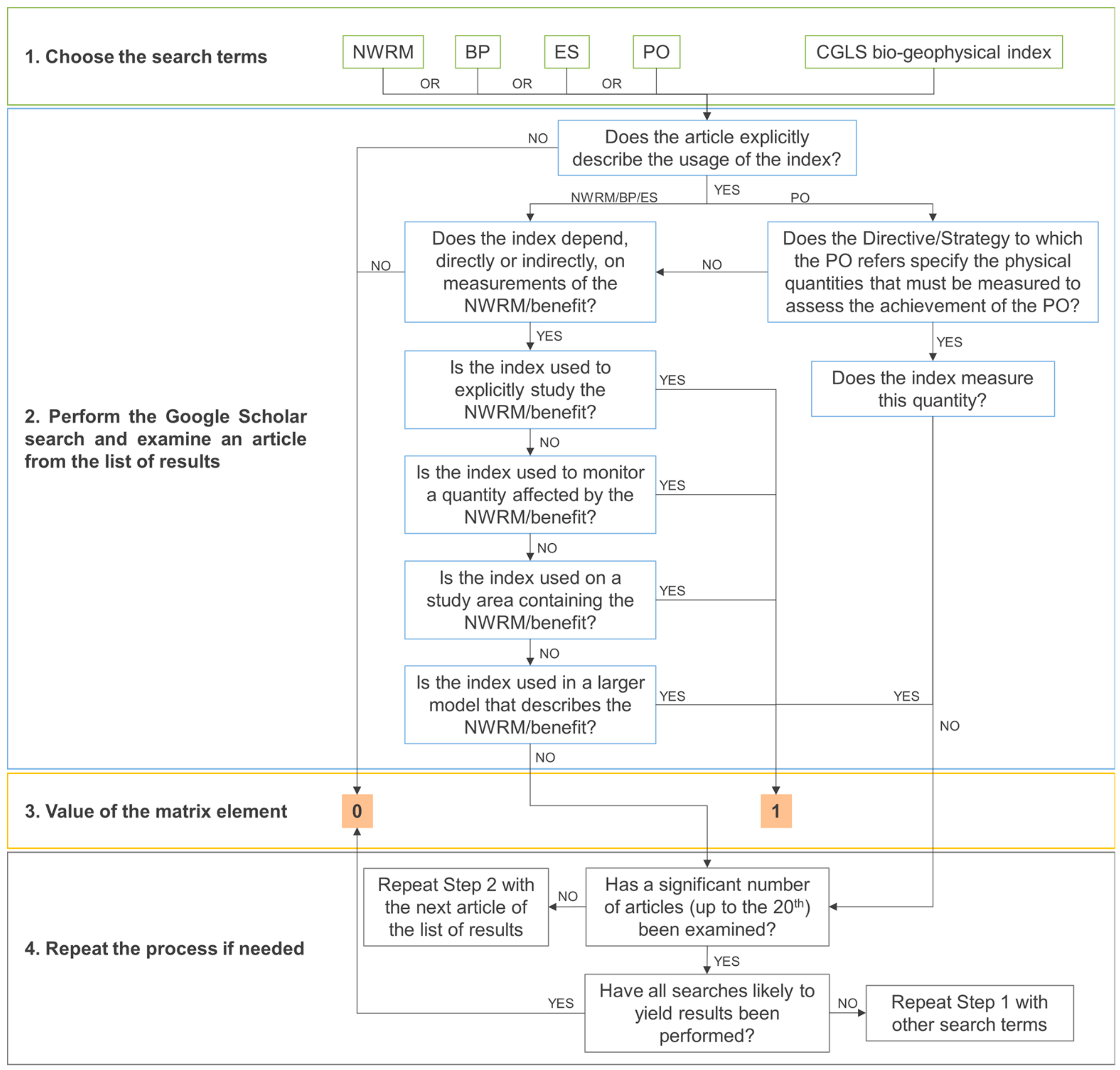
2.2.2. Literature Review

Having established a catalogue of the relevant NWRMs and related benefits (Section 2.1), we proceeded to perform a review of the scientific literature in order to estimate the potential of the vegetation and energy indices provided in the CGLS products to:
  • Study natural water retention measures (NWRMs).
  • Monitor their biophysical impacts (BPs).
  • Observe the delivery of NWRM-linked ecosystem services (ESs).
  • Assess the achievement of NWRM-related policy objectives (POs) expressed by EU directives and strategies.
Thus, we searched for scientific articles using the Google Scholar search engine, attesting whether a certain index had already been used, directly or indirectly, to detect or monitor the items in our catalogue. Google Scholar was the chosen tool to make the queries since more advanced bibliographical search engines display results based on the authors’ names, the title of the article, and keywords that the article is associated with. However, the main title and the keywords usually concern the main topic or the final results of the research, rather than the followed methodology.
The querying procedure entailed, first, the choice of the search terms: Typing the name of a specific vegetation or energy index among those provided by the CGLS (Table 3) along with a word or expression describing one of the catalogued NWRMs, BPs, ESs, or POs (Table 1 and Table 2). The search then yielded a list of articles, each of which was critically analyzed to ascertain whether it proved that the index had actually been used, or could be potentially used, to study the NWRM, BP, ES, or PO.
To critically decide whether an article actually proved a link between an index and a NWRM or benefit, a number of criteria were established, as described in step 2 of the followed procedure (Figure 2). It should be noted that a valid article did not necessarily have to cite the Copernicus program, nor did the indices it used have to be calculated using remote sensing data. It was also not necessary for a valid article to explicitly mention GIs or NWRMs or explicitly discuss ecosystem services and policy objectives.
The results of the literature review (i.e., the proven link between an index and a NWRM or benefit) were represented in a matrix form: Six matrices were prepared, displaying the links to CGLS products respectively of agriculture NWRMs, forest NWRMs, hydro-morphology NWRMs, BPs, ESs, and POs. Thus, each matrix cell corresponded to a given type of NWRM or related benefit and to a CGLS index. Should at least one article be found to prove a link between the two items, the cell value would be 1, else it would be 0.

2.3. Quality of CGLS Products

To obtain the final diagrams, we did not only assess, by reviewing the scientific literature, the actual or possible link between the bio-geophysical indices and each of the NWRMs and their resulting benefits; we also evaluated the quality that users could expect when using CGLS products. We thus carried out a well-grounded study of each vegetation and energy product, studying in deep detail the validation and accuracy assessment reports and user guides as of November 2018 [40,46,47,48,49,50,51,52,53,54,55,56,57,58,59,60,61,62,63,64,65,66,67,68,69] to fully understand the input data used, the algorithm developed, and the resulting output product. Using this information, a quality assessment was formulated for each version of every available product, which is shown in Table 4.
As previously shown in Table 3, almost all vegetation indices from CGLS offer two products with different spatial resolutions (SRs), either of 300 m or 1 km, except for VCI and VPI, currently just calculated using the NDVI 1 km product, and SWI, with a 25 km SR. On the other hand, energy indices are available with either 1 km (surface albedo and TOCR) or 5 km (LST) SRs. As for their temporal resolution (TR), almost all products are acquired every 10 days. NDVI 1 km, SWI, and LST offer both near-real time data and long-term composites with different TRs. Specifically, the NDVI 1 km product provides data every 10 days but also as a 6-month composite; the SWI product gives new data daily, every 10 days, as statistic composites and every 6 months as time series; and finally, LST is available hourly, daily, and every 10 days as composites of the daily values.
The quality was assessed on the basis of the product continuity, spatial and temporal consistencies, and accuracy and according to the categories of good, acceptable, moderate, or poor, as used along the consulted reports from the CGLS. The product continuity depended on the existence of large fractions of missing values or noisy and unreliable distributions around the globe, with no correlations between homogeneous sites. Thus, some products showed a bad continuity due to not properly covering the entire globe, showing large fractions of missing values in Northern latitudes, equatorial areas, and during winter time.
On the other hand, spatial and temporal consistencies measured whether there were large discrepancies between values relative to homogeneous areas and consecutive dates, respectively. The temporal consistency also took into account whether the temporal profiles were smooth or noisy. As for the accuracy, it was considered poor when values were either over or under-estimated compared to ground-truth data [45] or MODIS products [44]. For instance, FCOVER showed a poor accuracy over flooded vegetation, but positive results for bare and harvested areas, in comparison with FCOVER calculated with MODIS satellite sensor, according to the consulted reports [46,47,48].
Overall, the quality assessment was either good or acceptable for most of the products, being poor mainly for the newest versions of 300 m SR and still in the “demonstration” stage, such as FAPAR, FCOVER, LAI, or DMP [46,47,48,53]. That said, FCOVER remains a good candidate for replacing classical vegetation indices for the monitoring of ecosystems due to its sensitiveness to the vegetation amount without depending on the illumination direction [34].
As for the FAPAR and LAI 300 m versions, they showed poor or acceptable product continuity and spatial and temporal consistencies, but accuracy was good when comparing values with reference data [46,47,48]. VCI and VPI directly depend on the NDVI 1 km product and hence on the length of historical series available, the cloud contamination in the dataset, or existence of snow, which sometimes leads to below normal values, not corresponding to low vegetation activity, of all the indices. Hence, the user should always consider new products and see if the trend persists [50,51,52].
As for the energy indices, the overall quality was good. A “poor” assessment was given only to the product continuities of surface albedo and TOCR due to missing values over Northern latitudes and equatorial areas in wintertime. Spatial consistencies were considered acceptable since reliable and consistent values are obtained globally but unrealistic values result when analyzing locally snowy or cloudy areas. The temporal profiles, finally, are reliable when comparing PROBA-V, SPOT-VGT, and MODIS values, showing a good intra-annual precision [66,67,68,69].

2.4. Diagrams

The results of the literature review (Section 2.2) and the quality assessments (Section 2.3) were represented through Sankey diagrams. Moreover, since interpreting results derived from Sankey diagrams might be difficult due to the significant amount of illustrated information, even though the foremost aspects are easily visualized, user-friendly flowcharts were also produced.

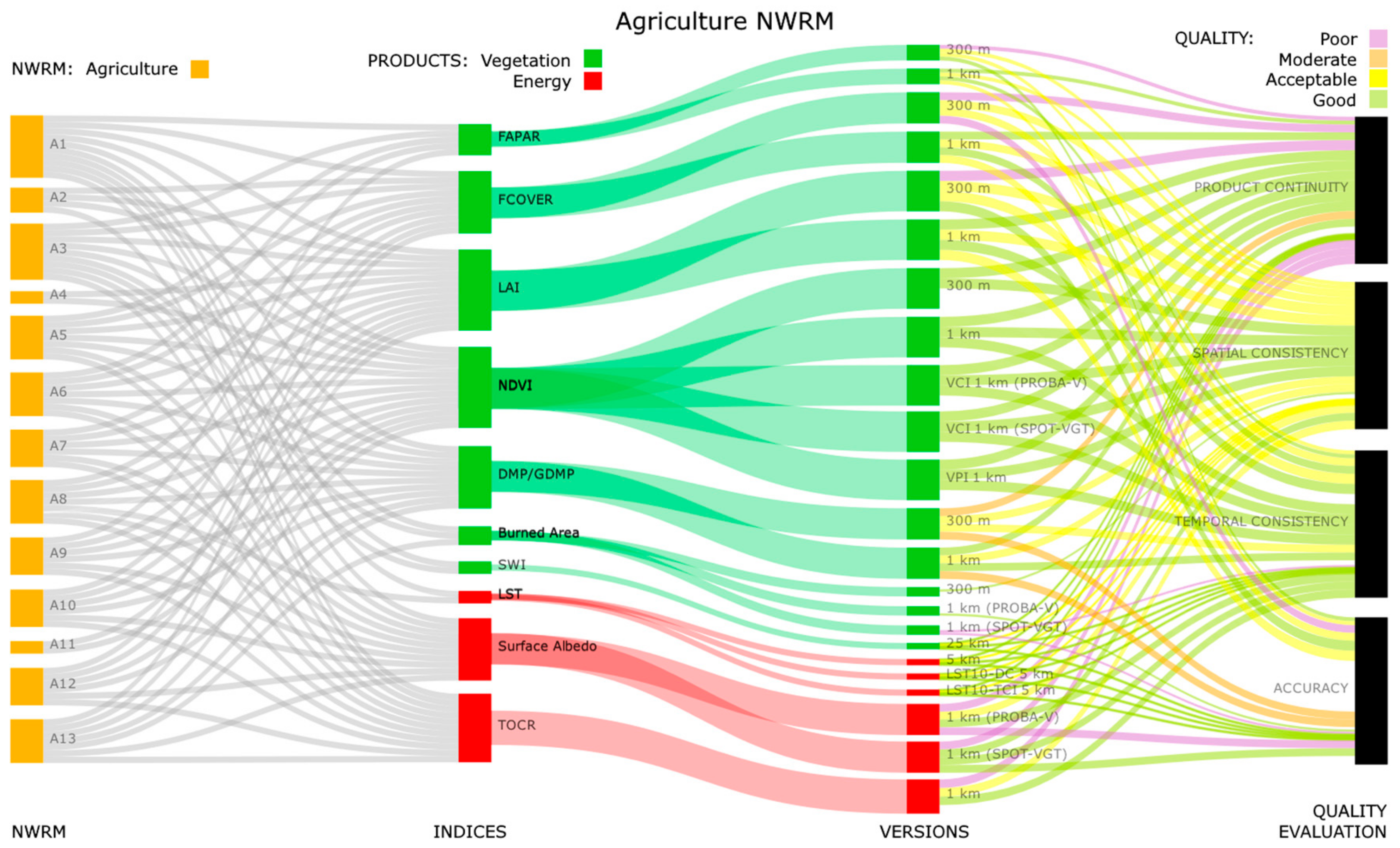
2.4.1. Sankey Diagrams

A Sankey diagram is a particular type of flow diagram. Within such a diagram, entities (nodes) are represented by rectangles or text, connected by lines whose thickness expresses the quantitative relationship between them. These diagrams are particularly suited to represent results organized in matrices [70]. Plotly was the chosen tool to construct the Sankey diagrams since it supported coding in Python [71]. Six Sankey diagrams were constructed, one for each of the matrices obtained from the literature review (Section 2.2) (Table 5).
Each diagram is arranged in 4 columns. The columns contain nodes corresponding to, from left to right: (i) catalogued agriculture NWRMs, forest NWRMs, hydro-morphology NWRMs, ESs, BPs, or POs; (ii) bio-geophysical indices provided by the CGLS vegetation and energy products; (iii) product versions depending on the available spatial resolutions; and (iv) characteristics considered in the quality assessments (see for example Figure 3, representing the agriculture NWRM diagram).
The nodes in the two leftmost columns are linked by lines, which mirror the cells of the matrix to which the Sankey diagram is related: If the value of a matrix cell (Tij), concerning an i-th index and a j-th NWRM, ES, BP, or PO, is equal to 1, a line linking the respective nodes exists, whereas if Tij is equal to 0, no such line is represented. The index nodes in the second column are then connected to their available versions, as provided by CGLS, in the third column. Finally, these versions are linked to the quality assessment parameters in the fourth column via color-coded lines: The line color indicates whether a product version has been evaluated with respect to a particular parameter as poor, moderate, acceptable, or good (Table 4).
It is worth mentioning that the NDVI node in the second column is linked to nodes in the third column relative to the available NDVI, VCI, and VPI versions, in light of the fact that the two latter products are derived directly from the former [40,50,51,52].
The width of each node of the three leftmost columns (represented as N j , P i , and V ik , corresponding to NWRM or benefits, indices, and versions, k being the product version number) depends on the following equations (Equations (1)–(3)):
N j = i T ij ,
P i = j T ij ,
V ik = 1 2 P i ,   k .
Thus, the width of a NWRM, BP, ES, or PO node depends on how many indices have been indicated by previous scientific works to be suitable for the direct or indirect study of the said NWRM, BP, ES, or PO. The width of an index node, on the other hand, shows how many NWRMs, BPs, ESs, or POs that index can study, again on the basis of previous research works.

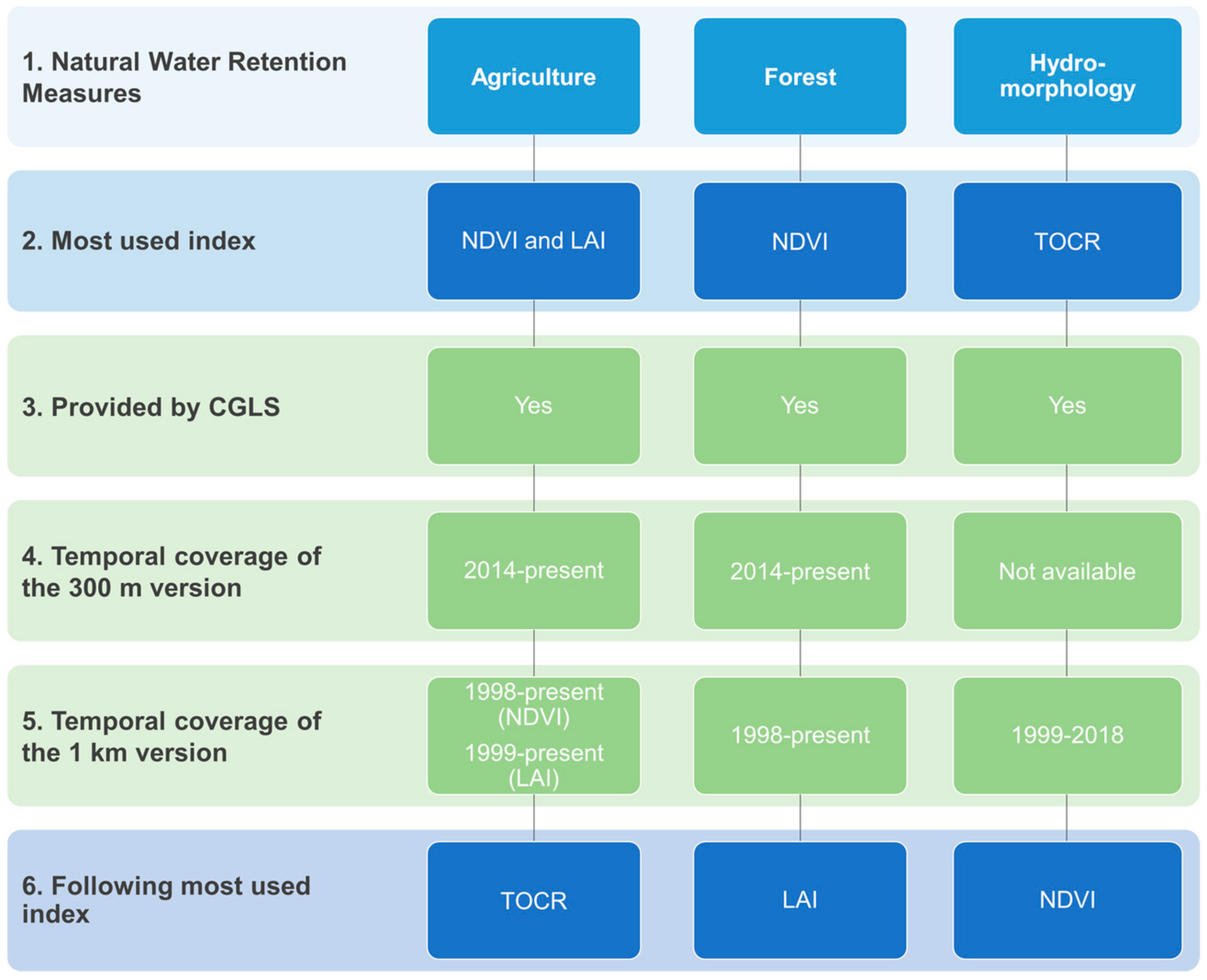
2.4.2. User-Friendly Flowcharts

With the aim of merging all the information and assisting actual GI users in selecting the potentially most suitable remotely-sensed bio-geophysical indices for analyzing NWRMs and their benefits, we designed user-friendly decision flows. These flowcharts lead from a given category of NWRMs, BPs, ESs, or POs to the CGLS index that is most appropriate for studying a wider variety of items belonging to the aforementioned category, on the basis of previous scientific research, and inform the user on the spatial resolution and temporal coverage (which is important for long time-series analyses) that are available in CGLS.

3. Results

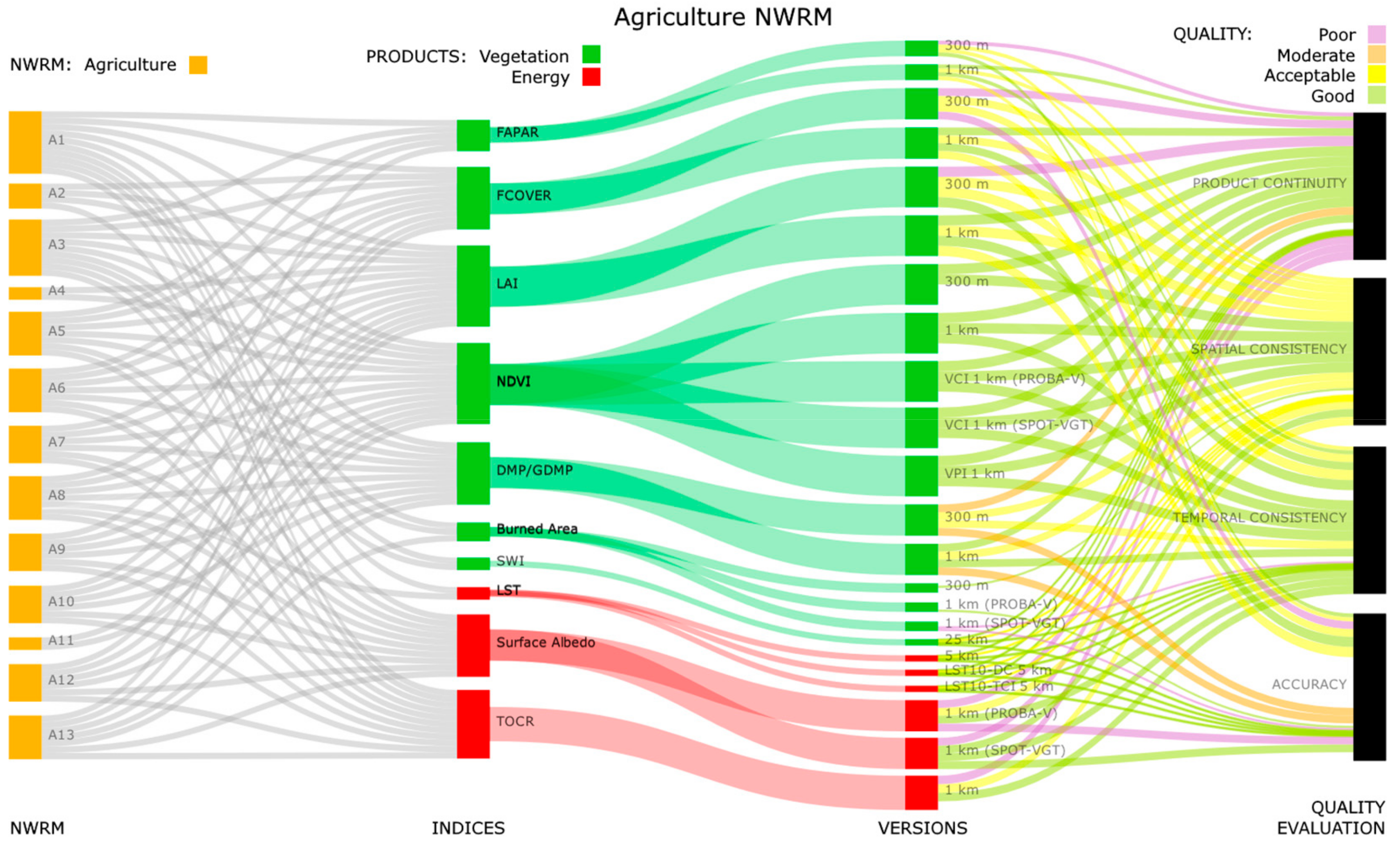
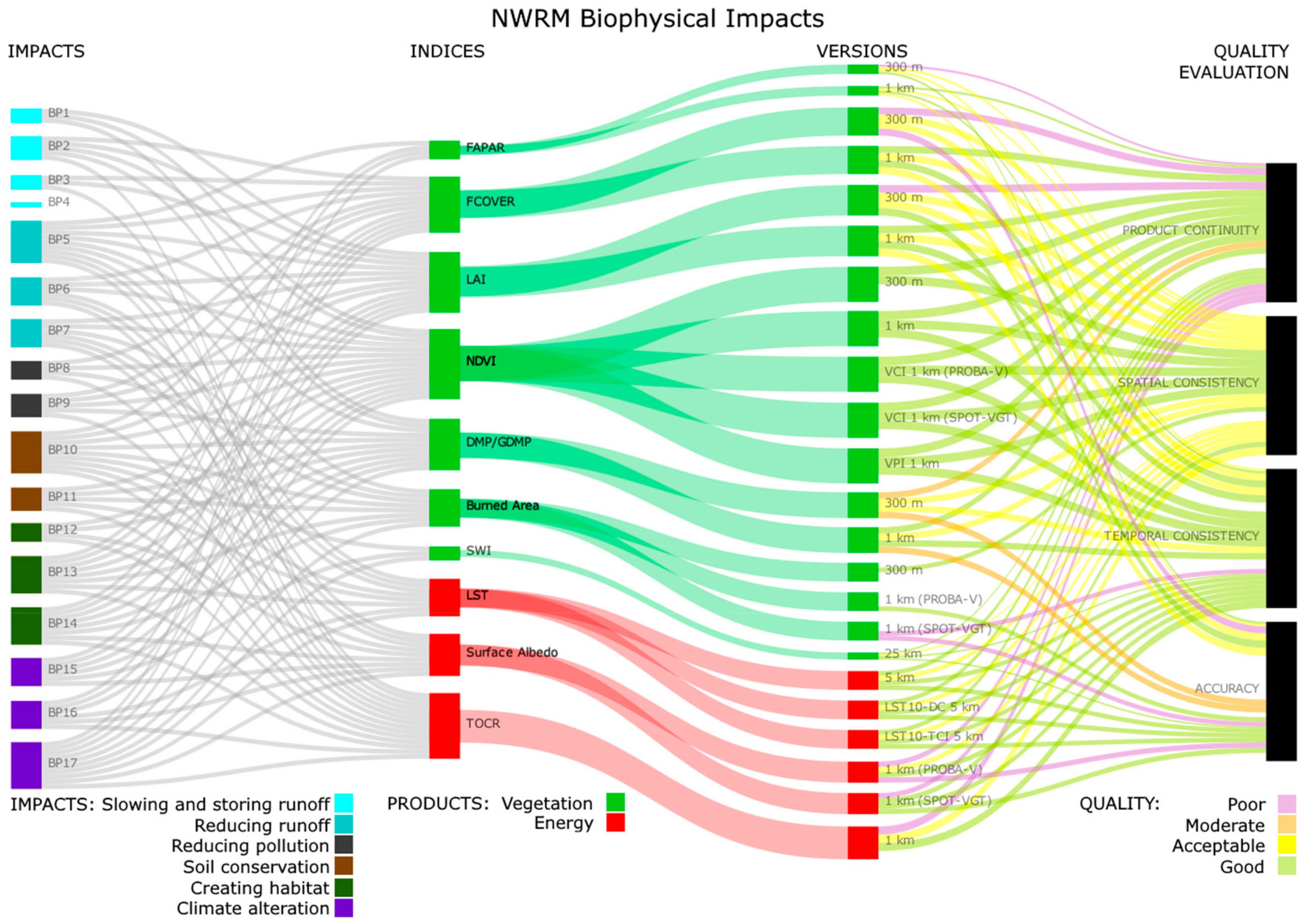
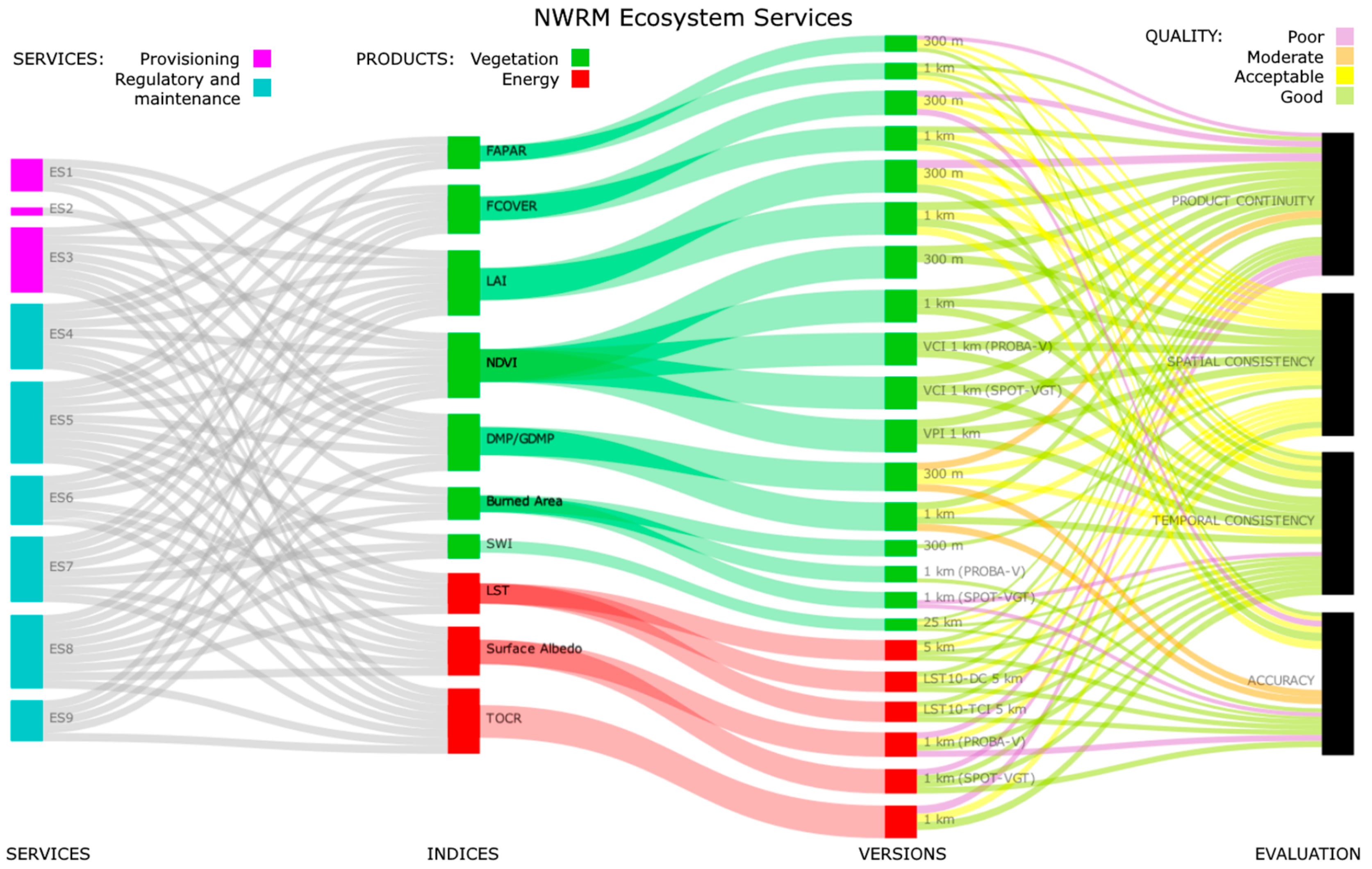
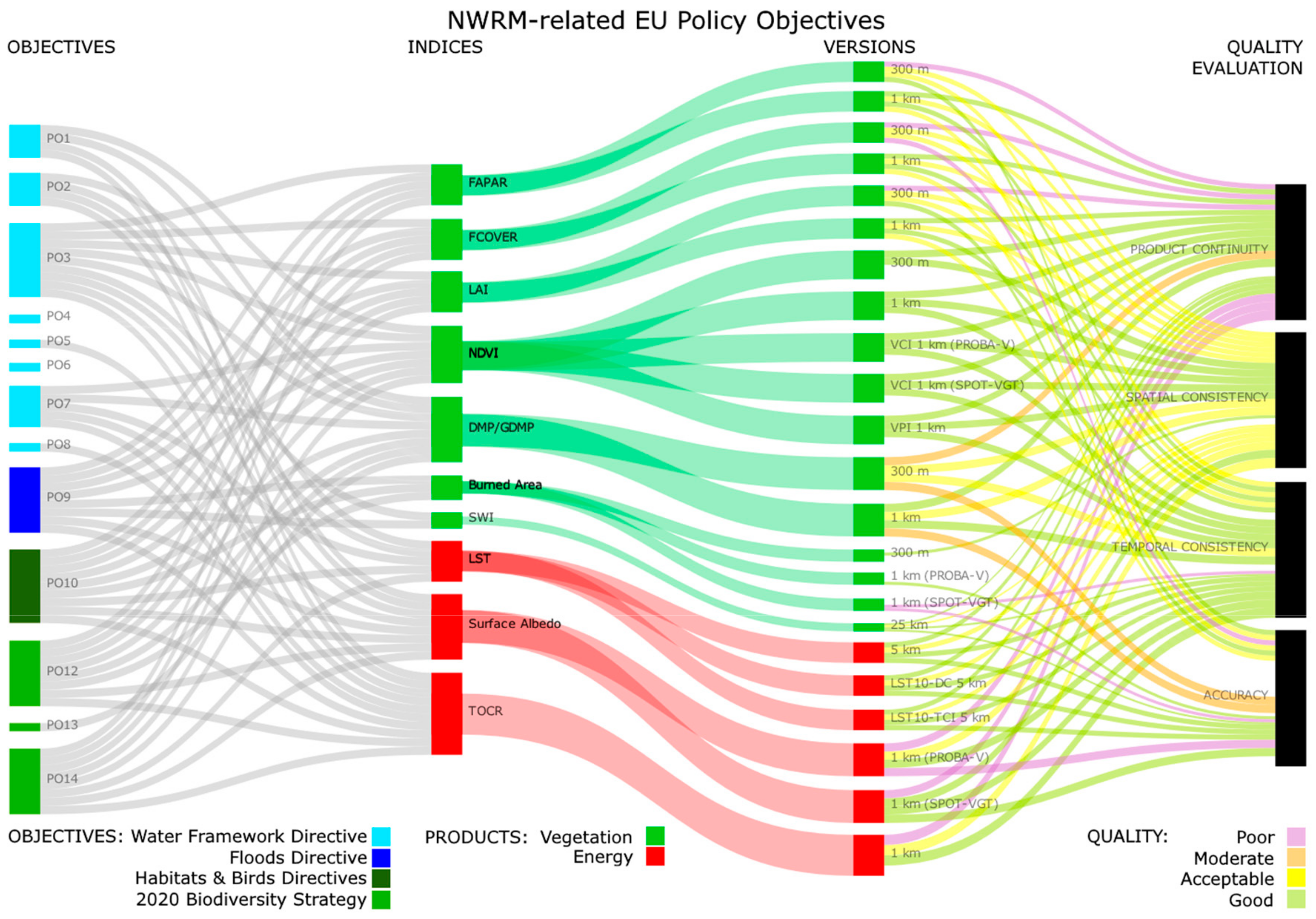
3.1. Interpreting the Sankey Diagrams

The main result of the work that we performed is the linking of the vegetation and energy indices freely available in the CGLS to NWRMs, BPs, ESs, and POs, on the basis of scientific articles that were found through a deep literature review. Sankey diagrams are useful to visualize the proportional flow and relationships between the different nodes within a network. They were thus well-suited to the representation of the above-mentioned links.
The six diagrams designed are meant to quickly show which vegetation and energy indices, available from the CGLS products, appear as the most suitable (according to previous research works) for the study and monitoring of NWRMs, ESs, BPs, and POs. Moreover, the diagrams show the quality that can be expected when employing the various versions of the CGLS products.
All the produced Sankey diagrams are displayed in Appendix A. As an example to interpret them, Figure 3 shows explicitly the diagram for the agriculture NWRMs. The linking lines between the nodes of the two leftmost columns (respectively representing the agriculture NWRMs and the bio-geophysical indices and hence their connection according to the reviewed works) are based on the matrix shown in Table 5, and hence on the cell values being either 1 or 0, as explained in detail in Section 2.4.1. The links with the two other columns are instead based on the data displayed in Table 4.
Overall, the diagram reveals, by analyzing each node width and the links between them along the different columns, the following information:
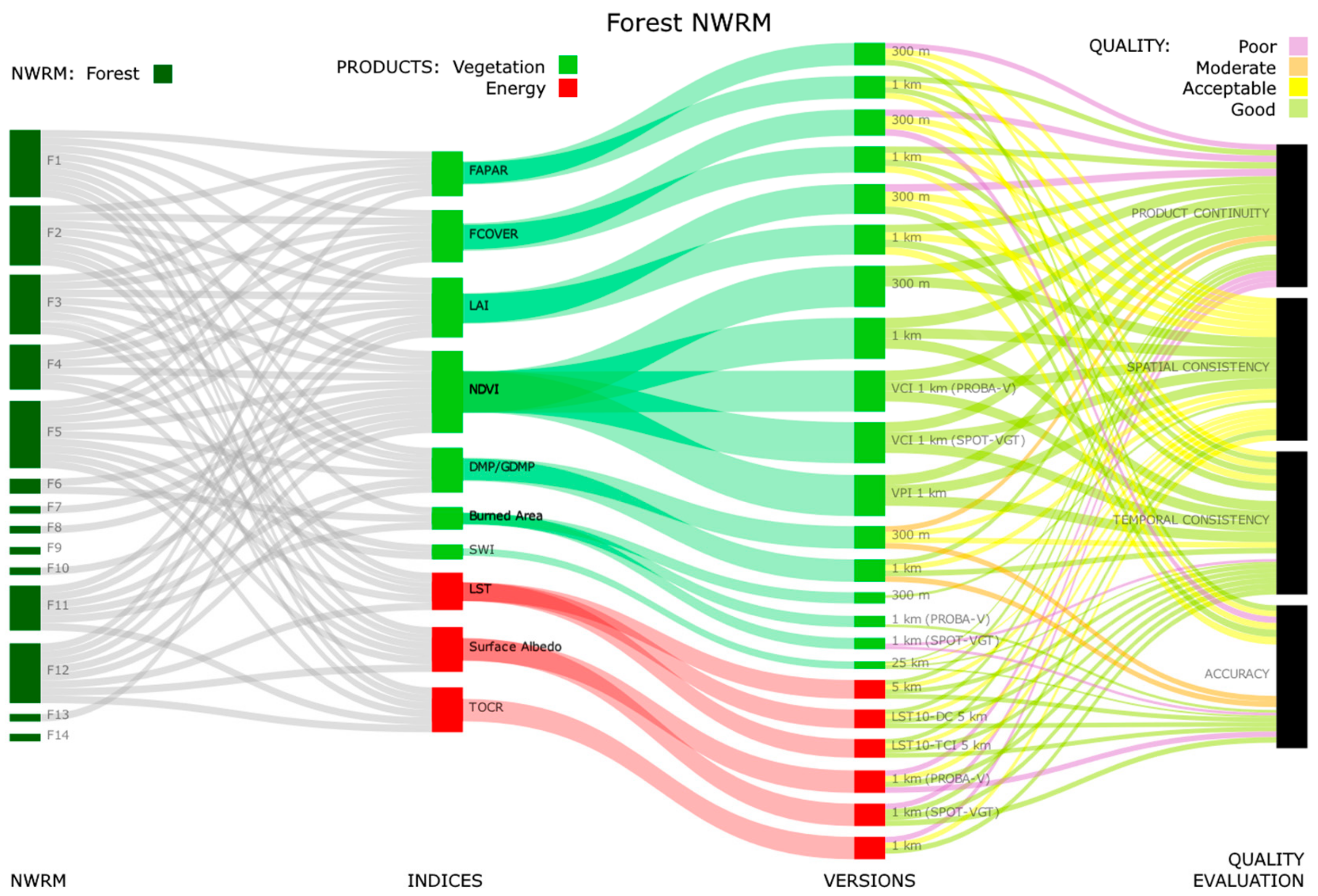
  • Which NWRMs or benefits (Table 1 and Table 2) have been successfully connected to the greatest number of bio-geophysical indices. This information can be ascertained from the widths of the diagram’s nodes of the leftmost column. In this specific diagram, the agriculture NWRMs that were suitably highlighted using most of the CGLS indices are meadows and pastures (A1) and crop rotation (A3), while solely two links and just with vegetation indices were found for strip cropping along contours (A4) and controlled traffic farming (A11).
  • Which CGLS vegetation indices have been used to identify and monitor the greatest number of NWRMs and benefits. The width of the green nodes of the second column, which depends on the number of connections to the nodes of the first column (i.e., how many NWRM or benefits each bio-geophysical index can actually or potentially study, according to the scientific literature), communicates this information.
    In this diagram, the normalized difference vegetation index (NDVI) and the leaf area index (LAI) are the vegetation indices showing the largest number of links to agriculture NWRMs and hence the greatest width, which implies they are capable of studying a wider variety of agriculture NWRMs. They are followed by the fraction of vegetation cover (FCOVER) and the dry matter productivity (DMP)/gross dry matter productivity (GDMP). The burned area and soil water index (SWI) are the least used vegetation indices.
  • The most used CGLS energy indices. The width of the red nodes of the second column, which depends again on the number of linking lines leading to them and hence on the indices’ suitability to monitor the NWRM or benefits in the first column, conveys this information.
    In this case, top-of-canopy reflectance (TOCR) is the energy index with the largest width and thus is capable of monitoring more agriculture NWRMs, closely followed by surface albedo. On the other hand, land surface temperature (LST) appears as the least used energy index.
  • The available versions (depending on the existing spatial resolutions) and the quality that users can expect when using the products. This information is shown in the third and fourth columns.
    Most of the products show a proper continuity along the globe with a minor amount of lost data, especially in Southern latitudes and during summertime, and a good temporal consistency for long-term analysis, with smooth temporal profiles (green lines). As for the spatial consistency, it is acceptable (yellow lines) for more than half of the products, with discrepancies when comparing values between homogeneous areas. Accuracy varies widely and has not been assessed for a significant number of product versions (Table 4). It is worth highlighting that the lines connecting the third and fourth columns are equivalent in all six Sankey diagrams.

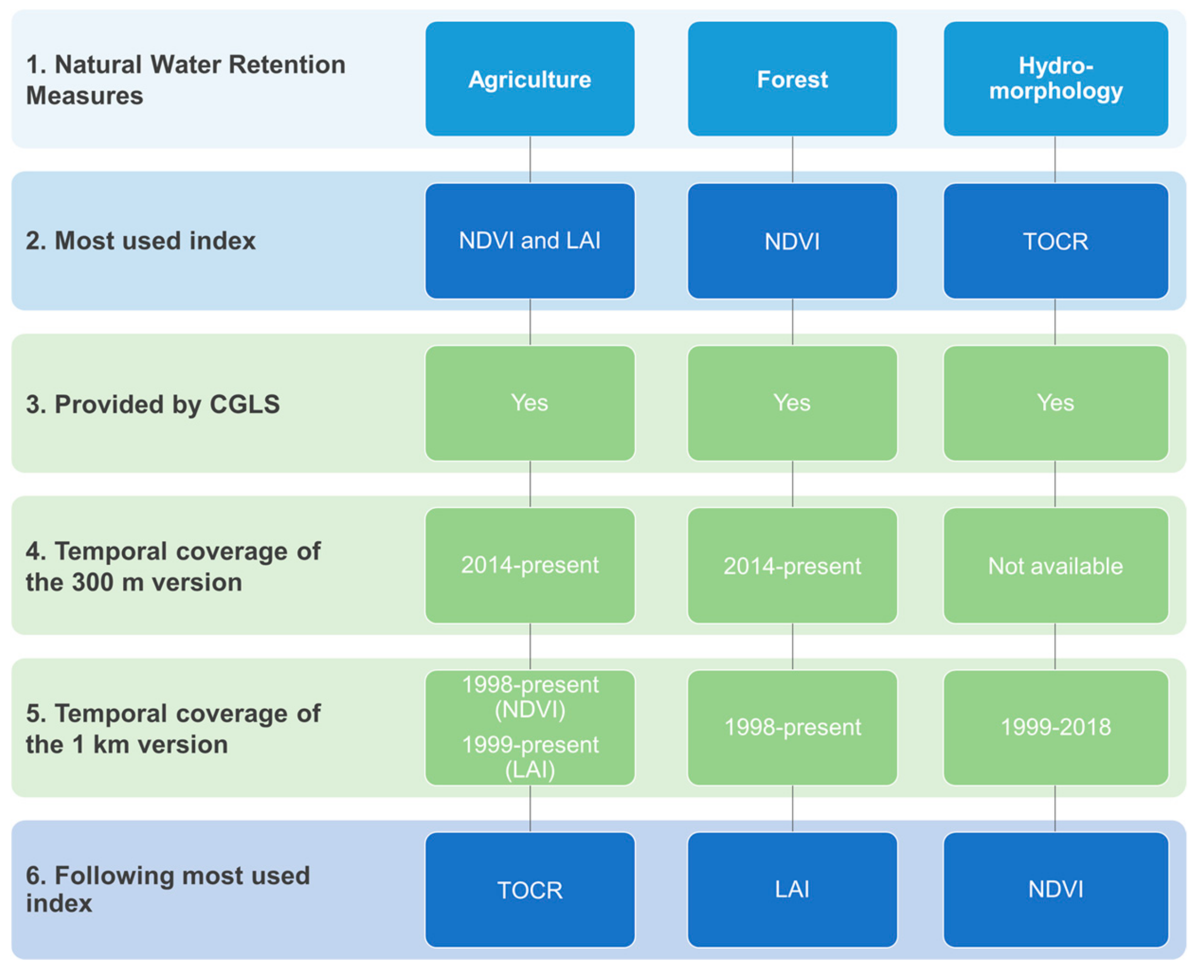
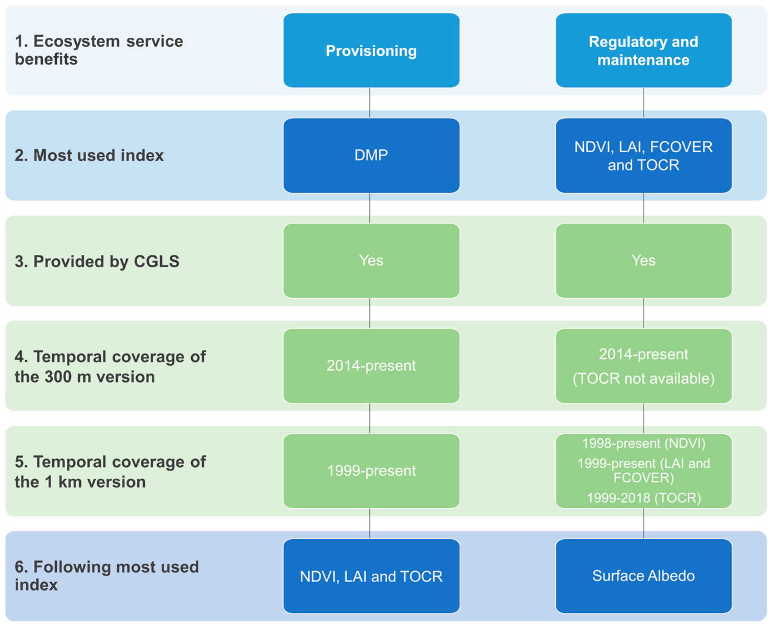
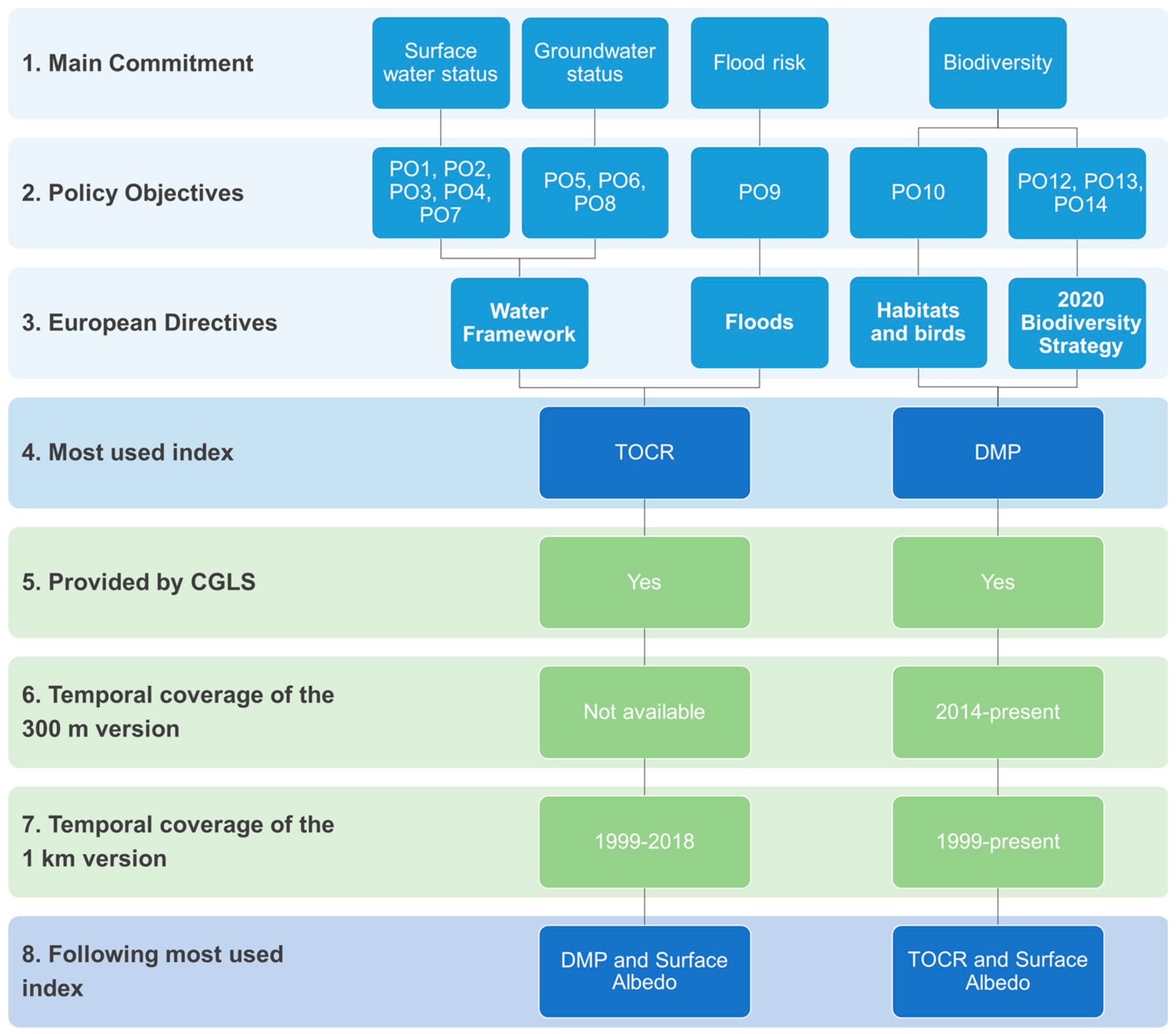
3.2. Understanding the User-Friendly Flowcharts

As previously mentioned, Sankey diagrams display such a large amount of information that we deemed it necessary to create more easy-to-read flowcharts to show just the most substantial results. All these charts are held in Appendix B and their aim is to help users in their decision-making tasks by indicating solely the most appropriate indices (according to the reviewed research works) for the monitoring of each category of items (NWRMs, BPs, ESs, and POs). The diagrams also show the temporal coverage of each version (300 m and 1 km) of these indices. This way, users can decide whether a better spatial resolution or a longer temporal coverage is preferable for their analyses and choose the most suitable product accordingly. Figure 4 is presented to illustrate how the final charts look.
Clearly, these flowcharts are easier to comprehend than Sankey diagrams, though it is the latter that truly hold all the outcomes of our research. This chart was specifically created for NWRM and shows that NDVI and LAI are both the indices that allow the monitoring of the greatest number of agriculture NWRMs. NDVI remains the index that lets us study the widest range of forest NWRMs, while TOCR is the recommended index for identifying hydro-morphology NWRMs. All the above-mentioned vegetation indices are available in the CGLS as two different products: 300 m and 1 km spatial resolutions; while TOCR is currently just offered as a 1 km product.

4. Discussion

Nowadays, supporting the development of nature-based measures, such as GIs or, more specifically, NWRMs, is very appreciated by policy makers since it contributes simultaneously to the achievement of several policy goals from water-related EU directives and climate change policies [10,12,13]. However, the lack of a well-grounded framework that allows the assessment of the multiple benefits of green infrastructures, including the improvement of the resilience of ecosystems, the achievement of policy goals, and cost-effectiveness, makes its implementation not yet truly operational [25,26]. Stakeholders and decision makers need to properly monitor and evaluate the effectiveness and impacts of the measures they are implementing [26,29,41]. Thus, aiming to support the successful implementation of NWRMs by promoting the use of the best available monitoring techniques, we reviewed the use of the bio-geophysical indices that are obtained from remotely-sensed earth observation data (and that are freely available in the CGLS [40]). Overall, they have proved to be certainly suitable to monitor most of the catalogued NWRMs, biophysical impacts, ecosystem services, and policy objectives (Table 2).
Analyzing both the final decision flowcharts (Appendix B) and the Sankey diagrams (Appendix A), some general trends can be noticed. For instance, NDVI is the most successfully used index, not only for the monitoring of agriculture and forest NWRMs but also for NWRM-related biophysical impacts. This is partly to be expected, given that this well-known parameter has actually been the most widely used vegetation index for decades, especially for monitoring vegetation health and growth [33,36,72,73], and hence an extensive scientific literature employing NDVI exists, starting from its first use in 1973 [74]. According to the reviewed articles, LAI also stands out as one of the most suitable indices for the monitoring of both agriculture NWRMs and “direct” biophysical impacts (slowing and storing run-off and reducing run-off), while TOCR is the following most used index in both categories (Figure 4 and Figure A8 in Appendix B).
Turning to the detection of the accomplishment of policy objectives from the Water Framework [22], Floods [24], Habitats [18], and Birds [19] EU Directives and the 2020 Biodiversity Strategy [16], it would appear that energy indices are the ones potentially most useful for this purpose. Specifically, TOCR is recommended for detecting the accomplishment of policy objectives linked to the first four directives, while DMP is the first choice for assessing the goals of the biodiversity strategy. In both cases, surface albedo is the following choice. Both TOCR and DMP have a very competitive temporal coverage, offering data from 1999 with 1 km spatial resolution globally. The main disadvantage of TOCR is that it is not available with a spatial resolution of 300 m yet (although we should point out that the TOCR 1 km version has been discontinued in 2018, awaiting the transition to Sentinel-2 data, which will solve this handicap) [40]. Thus, use of it would depend on the user’s needs: Desired level of detail and range of temporal coverage. The use of 300 m DMP products, which offer data from 2014, might be a better approach when analyses require a better spatial resolution (Figure A10 in Appendix B).
Regarding the delivery of ecosystem services, DMP stands out as the most recommended index for identifying NWRM-related provisioning services. On the other hand, a large set of indices is attested to be suitable for monitoring regulatory and maintenance services: NDVI, LAI, FCOVER, and TOCR. Except for TOCR, all indices are available in the CGLS as 300 m global products and data is offered from 1999 (1998 for NDVI) using 1 km versions [40] (Figure A9 in Appendix B).
It must be recognized that the bio-geophysical indices that appear to be the most recommended ones to identify and monitor NWRMs and their benefits are also the most consolidated, meaning that more scientific works employing them exist. FCOVER is an exception to this: It is a relatively new index, but it is considered as a promising replacement for classical vegetation indices [34,46,47,48] and this is visible in the developed diagrams, where its suitable use is frequently almost equivalent to LAI, NDVI, and DMP. On the other hand, FAPAR, burned area, and SWI seem to be overall the least used vegetation indices according to the literature review. Only in the Sankey diagram concerning the policy objectives addressed in the EU directives and the 2020 Biodiversity Strategy [16,18,19,22,24] does FAPAR show the same potential as FCOVER and LAI, mostly due to its links to biodiversity-related objectives (Figure A6 in Appendix A).
Let us now consider how suited NWRM and NWRM benefits are at being studied using CGLS products, which would definitely help in the framework of their truly operational implementation [25,26]. Agriculture NWRMs stand out as the nature-based measures for water retention that could be conceivably monitored through a larger set of bio-geophysical indices. This is especially true for meadows and pastures (A1) and crop rotation patterns (A3) (Figure A1 in Appendix A). Also, forest riparian buffers (F1) and land use conversion (F5) are linked to a high number of indices (Figure A2). It should be noted that riparian vegetated buffer strips have been widely discussed in the literature due to their ability to enhance and protect water quality, soil moisture, and river streams [15,75], more economically than would be possible to achieve through the implementation of traditional grey defenses [76].
On the other hand, no links were found for some forest-based measures, such as sediment capture ponds (F9) or overland flow areas in peatland forests (F14). A first hypothesis could be that this happens because energy and vegetation indices are not particularly suitable for the identification of hydrological features. However, wetland restoration and management (N2), floodplain restoration and management (N3), and restoration of natural infiltration to groundwater (N13) are hydro-morphology measures linked to a relatively large set of vegetation and energy indices (Figure A3). This fact highlights the potential of CGLS indices for the study of most NWRMs, even the aquatic ones. Thus, these apparently harder-to-monitor NWRMs might also be the least established in the scientific literature and hence hotspots to consider in future developments and research as pilot projects to test the hands-on condition and effectiveness of these NWRMs.
Our results thus show that NDVI and LAI are the indices that allow the monitoring of most NWRM-related biophysical impacts, as well as most agriculture and forest NWRMs. However, TOCR and DMP stand out as the most appropriate indices when studying the accomplishment of EU policy objectives, in line with the result obtained for NWRM-related ecosystem services.
A significant limitation of the present work that must be acknowledged is that our approach was solely reliant on the review of existing already-published literature. Thus, it could be argued that some NWRMs or related benefits could be monitored by more indices than those revealed by our review, even though no one has performed this analysis in the past [25,26,29,40]. It is even more likely that some of the newly developed bio-geophysical indices may have a great potential not yet assessed through scientific experiences. We are also aware that we might not have found articles linking the study of a given NWRM, ES, BP, or PO with the use of a certain index, in which case the matrices developed would contain false negatives (zeros).
Finally, users exploiting our results should not neglect to verify, even for highly recommended indices, that the available spatial and temporal resolutions are adequate to their needs. To this end, understanding the observation needs by collecting and consolidating GI users’ requirements will lead to maximization of their fulfilment [77].
In this sense, the temporal resolution of most of the CGLS products is very competitive, offering new data every 10 days at a global scale, which might fulfil the user requirements for any scale of their analyses and examined phenomenon. The issue of the spatial resolution is however more complex: CGLS products are currently available with either 300 m or 1 km spatial resolutions, which might or might not be acceptable for the users, highly dependent on the required level of detail. Thus, when GI users might need an analysis to be performed at a local level of detail, these products will almost surely not accomplish their requirements, which probably call for a spatial resolution of around 10 m (such a resolution is, for instance, currently provided by the Sentinel-2 MSI satellite sensor). It is for this reason that we advise that, as we analyzed in this work the suitability of the global Copernicus Land products for studying GIs/NWRMs and their benefits and policy goals, so should the appropriateness of the pan-European and local Copernicus products be assessed in future research, even if entailing different kinds of products [40].

5. Conclusions

From the obtained results, we are able to draw the following main conclusions:
  • Remotely-sensed satellite data keeps proving its high potential for monitoring the Earth, easing spatial planning and land use management tasks in large areas.
  • The examined vegetation and energy bio-geophysical indices, freely provided by the Copernicus Global Land Service (CGLS) products, are able to monitor most natural water retention measures (NWRMs) and their benefits, by which we mean NWRM biophysical impacts, delivered ecosystem services, and the accomplishment of NWRM-related policy objectives. Overall, the most suited vegetation indices are firstly the normalized difference vegetation index (NDVI) and secondly the leaf area index (LAI), while the most used energy index is top-of-canopy reflectance (TOCR).
  • We can thus see that the apparently most useful indices are the older ones, which can be used in a wide variety of contexts. NDVI remains the most suitable index based on the literature review.
  • Some newly-developed indices are also promising alternatives: The fraction of green vegetation cover (FCOVER), in particular, has shown its potential to replace or complement consolidated indices and we are implementing new research in that direction [78].
  • Just 8 out of the 80 catalogued NWRMs and related benefits were not linked to any index, which shows the indices’ potential for testing real NWRM pilot cases, providing a first baseline that, combined with future multidisciplinary research, eases the successful implementation of the same or similar measures. This may be due to: (i) No studies having been carried out on that specific subject or (ii) no indices being actually capable of monitoring the item. Future research could focus on studying this issue in detail.
  • Potential users should consider that the CGLS was not conceived as a database of complete and final products but as input data for researchers and institutions to develop new down-streaming services and evolve more detailed and scalable models, policies, strategies, planning, or management tools, with the aim of enhancing Earth monitoring and the detection of land changes and land uses, as well as assessing and encouraging the use of nature-based solutions for climate change adaptation.
  • The developed Sankey diagrams and final user-friendly flowcharts will hence help GI users in their decision-making tasks, providing information on the most suitable indices (according to the scientific literature) to monitor both NWRMs and their benefits. Moreover, the diagrams indicate the quality and accuracy that the user can expect when downloading and using the CGLS products.
  • The temporal coverage of the CGLS products is very competitive, particularly considering that most of them cover the globe every 10 days, surely fulfilling several users’ requirements on this regard, for any level of detail of their analyses. Also, most of the 1 km versions provide data from 1999, which allow studies using very long-term data series, also taking advantage of a good overall temporal consistency and data continuity along the globe, especially with almost no gaps during summertime and in Central and Southern latitudes. When instead analyzing data in Northern latitudes or wintertime, users should consider double-checking consecutive dates, homogeneous areas, and temporal profiles. Spatial consistency and accuracy should also be verified by the users, checking data from different sensors or for the same areas in several locations, since the reviewed technical documents show overall low, acceptable, or not-yet-assessed results for these two quality parameters.
  • Since Copernicus aims to meet the needs for ecosystem analyses on a global scale coming from national and regional public agencies countries and political/economic unions, such as the USA and the EU, a global and systematic acquisition system (i.e., able to acquire the Earth surface almost continuously and systematically with very competitive spatial resolutions) is a fundamental requirement for the Copernicus evolution. Specifically, referring to the spatial resolution, our study highlights the need for the Copernicus program to develop 300 m versions of all global indices, as this would make them considerably more useful, at least for intra-national and global scale analyses of the provided data. A coarse spatial resolution is unfortunately a significant handicap (e.g., as proven for the TOCR product). Accuracy assessments should also be provided for all the product versions.
  • The findings of this study are also valuable for the performance of a gap analysis between the available Copernicus products and operational user needs, as we are starting to work on [77]. Indeed, the European Commission has placed increasing interest in the collection of requirements to support the work of different institutional and private communities among the Member States. Thus, stakeholder needs, in terms of Copernicus products and services, can be identified through elicitation techniques and compared to the review hither performed in order to validate the information collected. This integration would provide the baseline not only for the advancement in technological provision, but also for the elaboration of policy recommendations in the domain of agriculture and environmental protection.

Author Contributions

Conceptualization, A.T. and E.V.; methodology, L.P., M.L., and A.T.; software, M.L.; validation, L.P., M.L., E.S., A.N.X., and E.V.; formal analysis, L.P. and M.L.; investigation, L.P. and M.L.; resources, L.P. and M.L.; data curation, L.P. and M.L.; all authors contributed to write, review, and edit the original manuscript; visualization, L.P., E.S., E.V., A.N.X., and A.T.; supervision, E.S., E.V., A.N.X., D.G.-A., and A.T.; project administration, A.T.; funding acquisition, A.T.

Funding

This research was funded by the European Commission, Directorate-General for European Civil Protection and Humanitarian Aid Operations (DG-ECHO), G.A. ECHO/SUB/2016/740172/PREV18. GREEN—Green infrastructures for disaster risk reduction protection: Evidence, policy instruments, and marketability.

Acknowledgments

The authors want to acknowledge the Institute for Advanced Study of Pavia (IUSS), the European Centre for Training and Research in Earthquake Engineering (Eucentre), and the Italian Institute for Environmental Protection and Research (ISPRA) for their help in achieving the goals of this project. The authors also want to thank the Spanish Ministry of Education, Culture, and Sports for providing an FPU grant (Training Program for Academic Staff) to the corresponding author of this paper.

Conflicts of Interest

The authors declare no conflict of interest.

Appendix A. Sankey Diagrams

This appendix contains all the Sankey diagrams derived from the presented review. Section 2.4.1 explained how these diagrams were developed. Each catalogued item was identified with an acronym (Table 1 and Table 2) while the main characteristics and quality assessment of the Copernicus Global Land Service (CGLS) products are shown in Table 4.
Figure A1. Sankey diagram linking the agriculture NWRM (A) and the CGLS vegetation and energy indices that are suitable for their monitoring, according to previous research experiences.
Remotesensing 11 01583 g0a1
Figure A2. Sankey diagram linking the forest NWRM (F) and the CGLS vegetation and energy indices that are suitable for their monitoring, according to previous research experiences.
Remotesensing 11 01583 g0a2
Figure A3. Sankey diagram linking the hydromorphology NWRM (N) and the CGLS vegetation and energy indices that are suitable for their monitoring, according to previous research experiences.
Remotesensing 11 01583 g0a3
Figure A4. Sankey diagram linking the vegetation and energy indices that according to previous experiences are suitable for monitoring the biophysical impacts (BP) resulting from the application of natural water retention measures (NWRMs).
Remotesensing 11 01583 g0a4
Figure A5. Sankey diagram linking the vegetation and energy indices that according to previous experiences are suitable for monitoring the ecosystem services (ES) delivered by natural water retention measures (NWRMs).
Remotesensing 11 01583 g0a5
Figure A6. Sankey diagram linking the vegetation and energy indices that according to previous experiences are suitable for monitoring the achievement of policy objectives (PO) through the application of natural water retention measures (NWRMs).
Remotesensing 11 01583 g0a6

Appendix B. Decision Flowcharts

This appendix contains all the final user-friendly flowcharts derived from the presented review. Section 2.4.2 explained how these diagrams were developed. Each catalogued item was identified with a short name (Table 1 and Table 2) while the main characteristics of the Copernicus Global Land Service (CGLS) products are shown in Table 3.
Figure A7. Decision flowchart indicating the most suitable indices available in the Copernicus Global Land Service for the monitoring of natural water retention measures.
Remotesensing 11 01583 g0a7
Figure A8. Decision flowchart indicating the most suitable indices available in the Copernicus Global Land Service for the monitoring of NWRM biophysical impacts.
Remotesensing 11 01583 g0a8
Figure A9. Decision flowchart indicating the most suitable indices available in the Copernicus Global Land Service for the monitoring of ecosystem services provided by NWRMs.
Remotesensing 11 01583 g0a9
Figure A10. Decision flowchart indicating the most suitable indices available in the Copernicus Global Land Service for the monitoring of the achievement of NWRM-related EU policy objectives.
Remotesensing 11 01583 g0a10

References

  1. Snäll, T.; Lehtomäki, J.; Arponen, A.; Elith, J.; Moilanen, A. Green Infrastructure Design Based on Spatial Conservation Prioritization and Modeling of Biodiversity Features and Ecosystem Services. Environ. Manag. 2016, 57, 251–256. [Google Scholar] [CrossRef] [PubMed]
  2. Cilliers, E.J. Reflecting on Green Infrastructure and Spatial Planning in Africa: The Complexities, Perceptions, and Way Forward. Sustainability 2019, 11, 455. [Google Scholar] [CrossRef]
  3. Artmann, M.; Kohler, M.; Meinel, G.; Gan, J.; Ioja, I.-C. How smart growth and green infrastructure can mutually support each other—A conceptual framework for compact and green cities. Ecol. Indic. 2019, 96, 10–22. [Google Scholar] [CrossRef]
  4. Evans, A.J.; Firth, L.B.; Hawkins, S.J.; Hall, A.E.; Ironside, J.E.; Thompson, R.C.; Moore, P.J. From ocean sprawl to blue-green infrastructure—A UK perspective on an issue of global significance. Environ. Sci. Policy 2019, 91, 60–69. [Google Scholar] [CrossRef]
  5. Lanzas, M.; Hermoso, V.; de-Miguel, S.; Bota, G.; Brotons, L. Designing a network of green infrastructure to enhance the conservation value of protected areas and maintain ecosystem services. Sci. Total Environ. 2019, 651, 541–550. [Google Scholar] [CrossRef]
  6. Lennon, M. Green infrastructure and planning policy: A critical assessment. Local Environ. 2015, 20, 957–980. [Google Scholar] [CrossRef]
  7. Maes, J.; Egoh, B.; Willemen, L.; Liquete, C.; Vihervaara, P.; Schägner, J.P.; Grizzetti, B.; Drakou, E.G.; La Notte, A.; Zulian, G.; et al. Mapping ecosystem services for policy support and decision making in the European Union. Ecosyst. Serv. 2012, 1, 31–39. [Google Scholar] [CrossRef]
  8. Maes, J.; Hauck, J.; Paracchini, M.L.; Ratamäki, O.; Hutchins, M.; Termansen, M.; Furman, E.; Pérez-Soba, M.; Braat, L.; Bidoglio, G. Mainstreaming ecosystem services into EU policy. Environ. Sustain. 2013, 5, 128–134. [Google Scholar] [CrossRef]
  9. European Commission. Communication from the Commission to the European Parliament, the Council, the European Economic and Social Committee and the Committee of the Regions; Green Infrastructure (GI)—Enhancing Europe’s Natural Capital, COM/2013/0249; European Commission: Brussels, Belgium, 2013. [Google Scholar]
  10. Hansen, R.; Olafsson, A.S.; van der Jagt, A.P.N.; Rall, E.; Pauleit, S. Planning multifunctional green infrastructure for compact cities: What is the state of practice? Ecol. Indic. 2019, 96, 99–110. [Google Scholar] [CrossRef]
  11. Valentini, E.; Filipponi, F.; Nguyen Xuan, A.; Passarelli, F.M.; Taramelli, A. Earth Observation for Maritime Spatial Planning: Measuring, Observing and Modeling Marine Environment to Assess Potential Aquaculture Sites. Sustainability 2016, 8, 519. [Google Scholar] [CrossRef]
  12. Cardoso da Silva, J.M.; Wheeler, E. Ecosystems as infrastructure. Perspect. Ecol. Conserv. 2017, 15, 32–35. [Google Scholar] [CrossRef]
  13. Suškevičs, M. Legitimate planning processes or informed decisions? Exploring public officials’ rationales for participation in regional green infrastructure planning in Estonia. Environ. Policy Gov. 2019, 29, 132–143. [Google Scholar] [CrossRef]
  14. Vallecillo, S.; Polce, C.; Barbosa, A.; Perpiña Castillo, C.; Vandecasteele, I.; Rusch, G.M.; Maes, J. Spatial alternatives for Green Infrastructure planning across the EU: An ecosystem service perspective. Landsc. Urban Plan. 2018, 174, 41–54. [Google Scholar] [CrossRef]
  15. Schindler, S.; Sebesvari, Z.; Damm, C.; Euller, K.; Mauerhofer, V.; Schneidergruber, A.; Biró, M.; Essl, F.; Kanka, R.; Lauwaars, S.G.; et al. Multifunctionality of floodplain landscapes: Relating management options to ecosystem services. Landsc. Ecol. 2014, 29, 229–244. [Google Scholar] [CrossRef]
  16. European Commission. Communication from the Commission to the European Parliament, the Council, the Economic and Social Committee and the Committee of the Regions; Our Life Insurance, Our Natural Capital: An EU Biodiversity Strategy to 2020, COM/2011/0244; European Commission: Brussels, Belgium, 2011. [Google Scholar]
  17. European Commission. Communication from the Commission to the European Parliament, the Council, the European Economic and Social Committee and the Committee of the Regions; An EU Strategy on Adaptation to Climate Change, COM/2013/0216; European Commission: Brussels, Belgium, 2013. [Google Scholar]
  18. European Commission. Council Directive 92/43/EEC of 21 May 1992 on the Conservation of Natural Habitats and of Wild Fauna and Flora; Official Journal L 206, 22/07/1992, 7–50; European Commission: Brussels, Belgium, 1992. [Google Scholar]
  19. European Commission. Directive 2009/147/EC of the European Parliament and of the Council of 30 November 2009 on the Conservation of Wild Birds; Official Journal L 20, 26/01/2010, 7–25; European Commission: Brussels, Belgium, 2010. [Google Scholar]
  20. European Commission. Communication from the Commission to the European Parliament, the Council, the European Economic and Social Committee and the Committee of the Regions; A New EU Forest Strategy: For Forests and the Forest-Based Sector, COM/2013/0659; European Commission: Brussels, Belgium, 2013. [Google Scholar]
  21. Common Agricultural Policy. Available online: https://ec.europa.eu/info/food-farming-fisheries/key-policies/common-agricultural-policy_en (accessed on 28 June 2018).
  22. European Commission. Directive 2000/60/EC of the European Parliament and of the Council of 23 October 2000 Establishing a Framework for Community Action in the Field of Water Policy; Official Journal L 327, 22/12/2000, 1–73; European Commission: Brussels, Belgium, 2000. [Google Scholar]
  23. European Commission. Directive 2006/118/EC of the European Parliament and of the Council of 12 December 2006 on the protection of groundwater against pollution and deterioration; Official Journal L 372, 27/12/2006, 19–31; European Commission: Brussels, Belgium, 2006. [Google Scholar]
  24. European Commission. Directive 2007/60/EC of the European Parliament and of the Council of 23 October 2007 on the Assessment and Management of Flood Risks; Official Journal L 288, 6/11/2007, 27–34; European Commission: Brussels, Belgium, 2007. [Google Scholar]
  25. Cools, J.; Strosser, P.; Achilleos, E.; Borchers, T.; Ochs, S.; Borchmann, A.; Steinmann, E.; Bussettini, M.; Gentili, M.M.; Gigliani, F.; et al. EU Policy Document on Natural Water Retention Measures; Technical Report; European Commission: Brussels, Belgium, 2014. [Google Scholar]
  26. Strosser, P.; Delacámara, G.; Hanus, A.; Williams, H.; Jaritt, N. A Guide to Support the Selection, Design and Implementation of Natural Water Retention Measures in Europe—Capturing the Multiple Benefits of Nature-Based Solutions, Final version, April 2015, Directorate—General for Environment; European Commission: Brussels, Belgium, 2016. [Google Scholar]
  27. Taramelli, A.; Valentini, E.; Cornacchia, L.; Bozzeda, F. A Hybrid Power Law Approach for Spatial and Temporal Pattern Analysis of Salt Marsh Evolution. J. Coast. Res. 2017, 77, 62–72. [Google Scholar] [CrossRef] [Green Version]
  28. European Commission. Directorate-General Environment. Towards Better Environmental Options for Flood Risk Management; Note by DG-ENV D.1. 2011/236452; European Commission: Brussels, Belgium, 2011. [Google Scholar]
  29. Pilot Project—Atmospheric Precipitation—Protection and Efficient Use of Fresh Water, Integration of Natural Water Retention Measures in River Basin Management. European Commission Directorate-General for Environment DG-ENV, 07.0330/2013/659147/SER/ENV.C1, 05/09/2013 to 05/11/2014. Available online: http://nwrm.eu/ (accessed on 16 July 2018).
  30. European Commission. Regulation (EU) No 377/2014 of the European Parliament and of the Council of 3 April 2014 Establishing the Copernicus Programme and Repealing Regulation (EU) No 911/2010 (Text with EEA Relevance). Journal L 122, 24/04/2014, 44–66; European Commission: Brussels, Belgium, 2014. [Google Scholar]
  31. Davies, C.; Lafortezza, R. Transitional path to the adoption of nature-based solutions. Land Use Policy 2019, 80, 406–409. [Google Scholar] [CrossRef]
  32. Tudorie, C.M.; Gielen, E.; Vallés-Planells, M.; Galiana, F. Urban green indicators: A tool to estimate the sustainability of our cities. Int. J. Des. Nat. Ecodyn. 2019, 14, 19–29. [Google Scholar] [CrossRef]
  33. Piedelobo, L.; Hernández-López, D.; Ballesteros, R.; Chakhar, A.; Del Pozo, S.; González-Aguilera, D.; Moreno, M.A. Scalable pixel-based crop classification combining Sentinel-2 and Landsat-8 data time series: Case study of the Duero river basin. Agric. Syst. 2019, 171, 36–50. [Google Scholar] [CrossRef]
  34. Filipponi, F.; Valentini, E.; Nguyen Xuan, A.; Guerra, C.A.; Wolf, F.; Andrzejak, M.; Taramelli, A. Global MODIS Fraction of Green Vegetation Cover for Monitoring Abrupt and Gradual Vegetation Changes. Remote Sens. 2018, 10, 653. [Google Scholar] [CrossRef]
  35. Murray, N.J.; Keith, D.A.; Bland, L.M.; Ferrari, R.; Lyons, M.B.; Lucas, R.; Pettorelli, N.; Nicholson, E. The role of satellite remote sensing in structured ecosystem risk assessments. Sci. Total Environ. 2018, 619–620, 249–257. [Google Scholar] [CrossRef]
  36. Piedelobo, L.; Ortega-Terol, D.; del Pozo, S.; Hernández-López, D.; Ballesteros, R.; Moreno, M.A.; Molina, J.-L.; González-Aguilera, D. HidroMap: A New Tool for Irrigation Monitoring and Management Using Free Satellite Imagery. ISPRS Int. J. Geo-Inf. 2018, 7, 220. [Google Scholar] [CrossRef]
  37. Bannari, A.; Morin, D.; Bonn, F.; Huete, A.R. A review of vegetation indices. Remote Sens. Rev. 1995, 13, 95–120. [Google Scholar] [CrossRef]
  38. Xue, J.; Su, B. Significant Remote Sensing Vegetation Indices: A Review of Developments and Applications. J. Sens. 2017, 1, 1–17. [Google Scholar] [CrossRef]
  39. Marando, F.; Salvatori, E.; Sebastiani, A.; Fusaro, L.; Manes, F. Regulating Ecosystem Services and Green Infrastructure: Assessment of Urban Heat Island effect mitigation in the municipality of Rome, Italy. Ecol. Model. 2019, 392, 92–102. [Google Scholar] [CrossRef]
  40. Copernicus Global Land Service. Providing Bio-Geophysical Products of Global Land Surface. Available online: https://land.copernicus.eu/global/index.html (accessed on 12 June 2018).
  41. GREEN Project—Green Infrastructures for Disaster Risk Reduction Protection: Evidence, Policy Instruments and Marketability. European Commission Directorate-General for European Civil Protection and Humanitarian Aid Operations DG-ECHO, ECHO/SUB/2016/740172/PREV18, 01/01/2017 to 31/12/2018. Available online: http://www.green-infrastructures.eu/ (accessed on 20 December 2018).
  42. Bjerklie, D.M.; Birkett, C.M.; Jones, J.W.; Carabajal, C.; Rover, J.A.; Fulton, J.W.; Garambois, P.-A. Satellite remote sensing estimation of river discharge: Application to the Yukon River Alaska. J. Hydrol. 2018, 561, 1000–1018. [Google Scholar] [CrossRef] [Green Version]
  43. Knipper, K.R.; Kustas, W.P.; Anderson, M.C.; Alfieri, J.G.; Prueger, J.H.; Hain, C.R.; Gao, F.; Yang, Y.; Mckee, L.G.; Nieto, H.; et al. Evapotranspiration estimates derived using thermal-based satellite remote sensing and data fusion for irrigation management in California vineyards. Irrig. Sci. 2018, 37, 431–449. [Google Scholar] [CrossRef]
  44. MODIS—Moderate-resolution Imaging Spectroradiometer. Available online: https://modis.gsfc.nasa.gov/ (accessed on 12 June 2018).
  45. LUCAS—Land Use and Land Cover Survey. Available online: https://ec.europa.eu/eurostat/statistics-explained/index.php/LUCAS_-_Land_use_and_land_cover_survey (accessed on 12 June 2018).
  46. Baret, F.; Weiss, M.; Lacaze, R.; Camacho, F.; Makhmara, H.; Pacholczyk, P.; Smets, B. GEOV1: LAI and FAPAR essential climate variables and FCOVER global time series capitalizing over existing products. Part1: Principles of development and production. Remote Sens. Environ. 2013, 137, 299–309. [Google Scholar] [CrossRef]
  47. Verger, A.; Baret, F.; Weiss, M. Near real-time vegetation monitoring at global scale. IEEE J. Sel. Top. Appl. Earth Obs. Remote Sens. 2014, 7, 3473–3481. [Google Scholar] [CrossRef]
  48. Camacho, F.; Cernicharo, J.; Lacaze, R.; Baret, F.; Weiss, M. GEOV1: LAI, FAPAR essential climate variables and FCOVER global time series capitalizing over existing products. Part 2: Validation and intercomparison with reference products. Remote Sens. Environ. 2013, 137, 310–329. [Google Scholar] [CrossRef]
  49. Toté, C.; Swinnen, E.; Sterckx, S.; Clarijs, D.; Quang, C.; Maes, R. Evaluation of the SPOT/VEGETATION Collection 3 reprocessed dataset: Surface reflectances and NDVI. Remote Sens. Environ. 2017, 201, 219–233. [Google Scholar] [CrossRef]
  50. Kogan, F.N. Remote sensing of weather impacts on vegetation in non-homogeneous areas. Int. J. Remote Sens. 1990, 11, 1405–1419. [Google Scholar] [CrossRef]
  51. Smets, B.; Eerens, H.; Jacobs, T.; Toté, C. Product User Manual—Vegetation Condition Index (VCI) and Vegetation Productivity Index (VPI). In GIO Global Land Component Lot I—Operation of the Global Land Component; GMES Initial Operations; Copernicus Global Land Service, European Commission: Brussels, Belgium, 2015. [Google Scholar]
  52. Sannier, C.A.D.; Taylor, J.C.; Du Plessis, W.; Campbell, K. Real-time vegetation monitoring with NOAA-AVHRR in Southern Africa for wildlife management and food security assessment. Int. J. Remote Sens. 1998, 19, 621–639. [Google Scholar] [CrossRef]
  53. Monteith, J.L. Solar Radiation and Productivity in Tropical Ecosystems. J. Appl. Ecol. 1972, 9, 747–766. [Google Scholar] [CrossRef]
  54. Padilla, M.; Olofsson, P.; Stehman, S.V.; Tansey, K.; Chuvieco, E. Stratification and sample allocation for reference burned area data. Remote Sens. Environ. 2017, 203, 240–255. [Google Scholar] [CrossRef]
  55. Padilla, M.; Stehman, S.V.; Chuvieco, E. Validation of the 2008 MODIS-MCD45 global burned area product using stratified random sampling. Remote Sens. Environ. 2014, 144, 187–196. [Google Scholar] [CrossRef]
  56. Padilla, M.; Stehman, S.V.; Ramo, R.; Corti, D.; Hantson, S.; Oliva, P.; Alonso-Canas, I.; Bradley, A.V.; Tansey, K.; Mota, B.; et al. Comparing the Accuracies of Remote Sensing Global Burned Area Products using Stratified Random Sampling and Estimation. Remote Sens. Environ. 2015, 160, 114–121. [Google Scholar] [CrossRef]
  57. Padilla, M.; Stehman, S.V.; Litago, J.; Chuvieco, E. Assessing the Temporal Stability of the Accuracy of a Time Series of Burned Area Products. Remote Sens. 2014, 6, 2050–2068. [Google Scholar] [CrossRef] [Green Version]
  58. Pekel, J.-F.; Cottam, A.; Gorelick, N.; Belward, A.S. High-resolution mapping of global surface water and its long-term changes. Nature 2016, 540, 418–422. [Google Scholar] [CrossRef]
  59. Tansey, K.; Gregoire, J.-M.; Stroppiana, D.; Sousa, A.; Silva, J.; Pereira, J.; Boschetti, L.; Maggi, M.; Brivio, P.A.; Fraser, R.; et al. Vegetation burning in the year 2000: Global burned area estimates from SPOT VEGETATION data. J. Geophys. Res. 2004, 109, D14. [Google Scholar] [CrossRef]
  60. Tansey, K.; Grégoire, J.-M.; Defourny, P.; Leigh, R.; Pekel, J.-F.; van Bogaert, E.; Bartholomé, E. A new, global, multi-annual (2000–2007) burnt area product at 1 km resolution. Geophys. Res. Lett. 2008, 35, 1–6. [Google Scholar] [CrossRef]
  61. Smith, R.; Adams, M.; Maier, S.; Craig, R.; Kristina, A.; Maling, I. Estimating the area of stubble burning from the number of active fires detected by satellite. Remote Sens. Environ. 2007, 109, 95–106. [Google Scholar] [CrossRef]
  62. FAO. Global Ecofloristic Zones Mapped by the United Nations Food and Agricultural Organization. 2000; Aaron, R., Gibbs, H.K., Eds.; FAO: Rome, Italy, 2008. [Google Scholar]
  63. Boschetti, L.; Roy, D.; Hoffmann, A.; Humber, M. MODIS Collection 5.1 Burned Area Product—MCD45. User’s Guide; Version 3.0.1. User Guide Ed.; Copernicus Global Land Service, European Commission: Brussels, Belgium, 2013. [Google Scholar]
  64. Albergel, C.; Rüdiger, C.; Pellarin, T.; Calvet, J.-C.; Fritz, N.; Froissard, F.; Suquia, D.; Petitpa, A.; Piguet, B.; Martin, E. From near-surface to root-zone soil moisture using an exponential filter: An assessment of the method based on in-situ observations and model simulations. Hydrol. Earth Syst. Sci. 2008, 12, 1323–1337. [Google Scholar] [CrossRef]
  65. Wagner, W.; Lemoine, G.; Rott, H. A Method for Estimating Soil Moisture from ERS Scatterometer and Soil Data. Remote Sens. Environ. 1999, 70, 191–207. [Google Scholar] [CrossRef]
  66. Freitas, S.C.; Trigo, I.F.; Macedo, J.; Barroso, C.; Silva, R.; Perdigão, R. Land Surface Temperature from multiple geostationary satellites. Int. J. Remote Sens. 2013, 34, 3051–3068. [Google Scholar] [CrossRef]
  67. Kogan, F.N. Operational Space Technology for Global Vegetation Assessment. Bull. Am. Meteorl. Soc. 2001, 82, 1949–1964. [Google Scholar] [CrossRef]
  68. Carrer, D.; Roujean, J.-L.; Meurey, C. Comparing Operational MSG/SEVIRI Land Surface Albedo Products From Land SAF with Ground Measurements and MODIS. IEEE. Trans. Geosci. Remote Sens. 2010, 48, 1714–1728. [Google Scholar] [CrossRef]
  69. Geiger, B.; Carrer, D.; Franchisteguy, L.; Roujean, J.-L.; Meurey, C. Land Surface Albedo Derived on a Daily Basis from Meteosat Second Generation Observations. IEEE. Trans. Geosci. Remote Sens. 2008, 46, 3841–3856. [Google Scholar] [CrossRef]
  70. Jentner, W.; Keim, D.A. Visualization and Visual Analytic Techniques for Patterns. In High-Utility Pattern Mining. Studies in Big Data; Fournier-Viger, P., Lin, J.W., Nkambou, R., Vo, B., Tseng, V., Eds.; Springer: Cham, Switzerland, 2019; Volume 51, pp. 303–337. [Google Scholar]
  71. Plotly. Modern Analytics Apps for the Enterprise. Available online: https://plot.ly/ (accessed on 3 September 2018).
  72. Immitzer, M.; Vuolo, F.; Atzberger, C. First Experience with Sentinel-2 Data for Crop and Tree Species Classifications in Central Europe. Remote Sens. 2016, 8, 166. [Google Scholar] [CrossRef]
  73. Inglada, J.; Arias, M.; Tardy, B.; Hagolle, O.; Valero, S.; Morin, D.; Dedieu, G.; Sepulcre, G.; Bontemps, S.; Defourny, P.; et al. Assessment of an Operational System for Crop Type Map Production Using High Temporal and Spatial Resolution Satellite Optical Imagery. Remote Sens. 2015, 7, 12356–12379. [Google Scholar] [CrossRef] [Green Version]
  74. Rouse, J.W.; Hass, R.H.; Schell, J.A.; Deering, D.W. Monitoring vegetation systems in the Great Plains with ERTS. In Third Earth Resources Technology Satellite-1 Symposium—Volume I: Technical Presentations; NASA SP-351; NASA: Washington, DC, USA, 1973; pp. 309–317. [Google Scholar]
  75. Zheng, H.; Li, Y.; Robinson, B.E.; Liu, G.; Ma, D.; Wang, F.; Lu, F.; Ouyang, Z.; Daily, G.C. Using ecosystem service trade-offs to inform water conservation policies and management practices. Front. Ecol. Environ 2016, 14, 527–532. [Google Scholar] [CrossRef]
  76. Tiwari, T.; Lundström, J.; Kuglerová, L.; Laudon, H.; Öhman, K.; Ågren, A.M. Cost of riparian buffer zones: A comparison of hydrologically adapted site-specific riparian buffers with traditional fixed widths. Water Resour. Res. 2016, 52, 1056–1069. [Google Scholar] [CrossRef] [Green Version]
  77. Tornato, A.; Valentini, E.; Nguyen Xuan, A.; Taramelli, A.; Schiavon, E. Assessment of User-Driven Requirements in term of Earth Observation Products and Applications for Institutional Operational Services. In AGU Fall Meeting Abstracts, Proceedings of the AGU Fall Meeting Washington, DC, USA, 10–14 December 2018; American Geophysical Union: Washington, DC, USA, 2018. [Google Scholar]
  78. Valentini, E.; Nguyen Xuan, A.; Filipponi, F.; Tornato, A.; De Peppo, M.; Taramelli, A. Pressures, Quality and Threats in European Protected Areas Evaluating Vegetation (FCover) Changes. In AGU Fall Meeting Abstracts, Proceedings of the AGU Fall Meeting, Washington, DC, USA, 10–14 December 2018; American Geophysical Union: Washington, DC, USA, 2018. [Google Scholar]
Figure 1. Flowchart showing the steps followed to determine the most recommended vegetation and energy indices provided by the Copernicus Global Land Service for monitoring natural water retention measures and their benefits.
Remotesensing 11 01583 g001
Figure 2. Flowchart of the followed procedure to perform each query and ascertain whether a given article was valid and effectively proved the existence of an actual or possible link between a bio-geophysical index and a NWRM, BP, ES, or PO.
Remotesensing 11 01583 g002
Figure 3. Sankey diagram linking the vegetation and energy indices to the agriculture NWRM that they can be employed to study and monitor, according to previous research works, and to their versions available in the Copernicus Global Land Service, which are in turn linked to expected quality. The short-names of the catalogued NWRM are explained in Table 1.
Remotesensing 11 01583 g003
Figure 4. Decision flowchart indicating the most suitable indices available in the Copernicus Global Land Service for the monitoring of natural water retention measures.
Remotesensing 11 01583 g004
Table 1. Catalogue of the studied natural water retention measures (NWRMs), based on the NWRM project [29]. Short-names in bold are the ones displayed in the final diagrams.
AgricultureForestHydro-Morphology
A1Meadows and pasturesF1Forest riparian buffersN1Basins and ponds
A2Buffer strips and hedgesF2Maintenance of forest cover in headwater areasN2Wetland restoration and management
A3Crop rotationF3Afforestation of reservoir catchmentsN3Floodplain restoration and management
A4Strip cropping along contoursF4Targeted planting for catching precipitationN4Re-meandering
A5IntercroppingF5Land use conversionN5Stream bed re-naturalization
A6No till agricultureF6Continuous cover forestryN6Restoration and reconnection of seasonal streams
A7Low till agricultureF7Water sensitive drivingN7Reconnection of oxbow lakes and similar features
A8Green coverF8Appropriate design of roads and stream crossingsN8Riverbed material
re-naturalization
A9Early sowingF9Sediment capture pondsN9Removal of dams and other longitudinal barriers
A10Traditional terracingF10Coarse woody debrisN10Natural bank stabilization
A11Controlled traffic farmingF11Urban forest parksN11Elimination of riverbank protection
A12Reduced stocking densityF12Trees in urban areasN12Lake restoration
A13MulchingF13Peak flow control structuresN13Restoration of natural infiltration to groundwater
F14Overland flow areas in peatland forestsN14Re-naturalization of polder areas
Table 2. Catalogue of the studied biophysical impacts, ecosystem services, and policy objectives linked to natural water retention measures, based on the NWRM project [29]. Short-names in bold are the ones displayed in the final diagrams.
Biophysical ImpactsEcosystem ServicesPolicy Objectives
BP1Store runoffES1Water storagePO1Improving status of biology quality elements (WFD)
BP2Slow runoffES2Fish stocks and recruitingPO2Improving status of physicochemical quality elements (WFD)
BP3Store river waterES3Natural biomass productionPO3Improve status of hydro-morphology quality elements (WFD)
BP4Slow river waterES4Biodiversity preservationPO4Improve chemical status and priority substances (WFD)
BP5Increase evapotranspirationES5Climate change adaptation and mitigationPO5Improve quantitative status (WFD)
BP6Increase infiltration and/or groundwater rechargeES6Groundwater/aquifer rechargePO6Improve chemical status (WFD)
BP7Increase soil water retentionES7Flood risk reductionPO7Prevent surface water status deterioration (WFD)
BP8Reduce pollutant sourcesES8Erosion/sediment controlPO8Prevent groundwater status deterioration (WFD)
BP9Intercept pollution pathwaysES9Filtration of pollutantsPO9Take adequate and coordinated measures to reduce flood risks (FD)
BP10Reduce erosion and/or sediment deliveryPO10Protection of important habitats (HD and BD)
BP11Improve soilsPO12More sustainable agriculture and forestry (BS)
BP12Create aquatic habitatPO13Better management of fish stocks (BS)
BP13Create riparian habitatPO14Prevention of biodiversity loss (BS)
BP14Create terrestrial habitat
BP15Enhance precipitation
BP16Reduce peak temperatures
BP17Absorb and/or retain CO2
Table 3. Main characteristics of the last-updated versions of the bio-geophysical indices considered in the literature review, provided by the Copernicus Global Land Service (CGLS) through its vegetation and energy products [40] (as of November 2018).
IndexSatellite SensorSpatial ResolutionTemporal ResolutionTemporal CoverageStage
VegetationFAPARPROBA-V300 m10 days01/2014–presentDemonstration
SPOT-VGT, PROBA-V1 km10 days01/1999–presentOperational
FCOVERPROBA-V300 m10 days01/2014–presentDemonstration
SPOT-VGT, PROBA-V1 km10 days01/1999–present
LAIPROBA-V300 m10 days01/2014–presentDemonstration
SPOT-VGT, PROBA-V1 km10 days01/1999–present
NDVIPROBA-V300 m10 days01/2014–presentOperational
SPOT-VGT, PROBA-V1 kmNRT 1: 10 days04/1998–present
LTS 2: 6 months01/1999–12/2017
VCIPROBA-V1 km10 days06/2014–presentDemonstration
SPOT-VGT1 km10 days01/2013–05/2014Operational
VPIPROBA-V1 km10 days06/2014–07/2017Demonstration
SPOT-VGT1 km10 days01/2013–05/2014Operational
DMP/GDMPPROBA-V300 m10 days01/2014–presentDemonstration
SPOT-VGT, PROBA-V1 km10 days01/1999–present
Burned AreaPROBA-V300 m10 days04/2014–presentPre-operational
PROBA-V1 km10 days04/2014–08/2018
SWIMETOP(A&B)/ASCAT25 kmSWI: 1 day01/2007–presentOperational
SWI10 3: 10 days01/2007–present
SWI-TS 4: 6 months01/2007–present
EnergyLSTMETEOSAT (MSG); GOES; MTSAT/Himawari5 kmLST: 1 hour10/2010–presentOperational
LST10-DC 3: 10 days01/2017–present
LST10-TCI 5: 10 days01/2017–present
Surface AlbedoPROBA-V1 km10 days05/2014–presentDemonstration
SPOT-VGT1 km10 days12/1998–04/2014Operational
TOCRSPOT-VGT, PROBA-V1 km10 days01/1999–08/2018Demonstration
1 Near-real time. 2 Long term statistics. 3 10-day statistics of daily values. 4 Reformatting to time series format of daily values. 5 Thermal condition index with 10-day composites.
Table 4. Quality and accuracy assessments of the bio-geophysical indices provided by the Copernicus Global Land Service (CGLS) vegetation and energy products, evaluating the product continuity, spatial consistency, temporal consistency, and accuracy as either good (G), acceptable (A), moderate (M), or poor (P) as in the consulted references [40] (as of November 2018).
IndexSpatial ResolutionProduct ContinuitySpatial ConsistencyTemporal ConsistencyAccuracyReferences
VegetationFAPAR300 mPAAG[46,47,48]
1 kmGAGA
FCOVER300 mPAAP[46,47,48]
1 kmGAGA
LAI300 mPAAG[46,47,48]
1 kmGAGA
NDVI300 mGG--[46,49]
1 kmGGG-
VCI1 km (SPOT-VGT)GGG-[50,51]
1 km (PROBA-V)GGG-
VPI1 kmGGG-[51,52]
DMP/GDMP300 mMAAM[53]
1 kmGAGM
Burned Area300 m-G--[54,55,56,57,58,59,60,61,62,63]
1 km (PROBA-V)---G
1 km (SPOT-VGT)--PP
SWI25 kmGAGG[64,65]
EnergyLST5 kmGAGG[66,67]
Surface albedo1 km (PROBA-V)PAGP[68,69]
1 km (SPOT-VGT)PGGG
TOCR1 kmPAG-[66,67]
Table 5. Matrix representing the links of the evaluated agriculture NWRM and CGLS. Cell values of 1 or 0 indicate, respectively, whether an article indicating the actual or potential use of a given index to monitor a given agriculture NWRM was found or not during the review of research works.
Agriculture NWRMFAPARFCOVERLAINDVIDMP/GDMPBurned AreaSWILSTSurface AlbedoTOCR
A11111111111
A20111000001
A31111111011
A40011000000
A51111100011
A61111100011
A70111100011
A80111100111
A91011100011
A100111100011
A110011000000
A120111100011
A130111110011

