Abstract
Strawberry growers in Florida suffer from a lack of efficient and accurate yield forecasts for strawberries, which would allow them to allocate optimal labor and equipment, as well as other resources for harvesting, transportation, and marketing. Accurate estimation of the number of strawberry flowers and their distribution in a strawberry field is, therefore, imperative for predicting the coming strawberry yield. Usually, the number of flowers and their distribution are estimated manually, which is time-consuming, labor-intensive, and subjective. In this paper, we develop an automatic strawberry flower detection system for yield prediction with minimal labor and time costs. The system used a small unmanned aerial vehicle (UAV) (DJI Technology Co., Ltd., Shenzhen, China) equipped with an RGB (red, green, blue) camera to capture near-ground images of two varieties (Sensation and Radiance) at two different heights (2 m and 3 m) and built orthoimages of a 402 m2 strawberry field. The orthoimages were automatically processed using the Pix4D software and split into sequential pieces for deep learning detection. A faster region-based convolutional neural network (R-CNN), a state-of-the-art deep neural network model, was chosen for the detection and counting of the number of flowers, mature strawberries, and immature strawberries. The mean average precision (mAP) was 0.83 for all detected objects at 2 m heights and 0.72 for all detected objects at 3 m heights. We adopted this model to count strawberry flowers in November and December from 2 m aerial images and compared the results with a manual count. The average deep learning counting accuracy was 84.1% with average occlusion of 13.5%. Using this system could provide accurate counts of strawberry flowers, which can be used to forecast future yields and build distribution maps to help farmers observe the growth cycle of strawberry fields.
1. Introduction
Strawberries are a high-value crop in the economy of Florida. Based on a report from the U.S. Department of Agriculture, the value of production for strawberries in Florida was $282 million in 2018, the second-largest in the United States [1]. The strawberry harvest season runs from December to April and, during this time, flowers form and become fruit in subsequent weeks. There may be some major “fruit waves”, in which the production yield can vary greatly from week to week [2]. Weather fluctuations are one of the main causes of this phenomenon. In the main production areas in central Florida, the mean daily temperature is 25 °C in early November, declining to 15 °C in the middle of January and rising to 21 °C in late April [3]. The day lengths and temperatures are conducive to flower bud initiation [4,5]. In Florida, the fruit development period typically extends from three weeks to six weeks as the day length declines and temperatures sink below the average [6,7].
Due to the dramatic fluctuation in weekly yields, strawberry growers need to monitor the fields frequently in order to schedule proper labor and equipment, as well as other resources for harvesting, transportation, and marketing [8,9,10]. Predicting yields quickly and precisely is vital for optimal management; particularly, to prevent farmers from suffering from insufficient labor. Accurate prediction can reduce the waste of the unpicked over-ripe fruit due to labor shortages in the best harvest time [11]. At present, yield estimation is done manually, which is very time-consuming and labor intensive. In the early 2000 s, researchers found some relationships between environmental factors and strawberry yields and tried to build models for yield prediction. Døving and Mage [12,13] found that the climate conditions had more impact on yield during flower induction and flower differentiation periods than during flowering and harvesting periods. By using historical yield data from 1967–2000 in Norway, they found a strong correlation between strawberry yield level and fungicides used against Botrytis cinerea. The correlation between yield levels and temperatures varied in different seasons [14]. Misaghi et al. [15] input the vegetation index, soil characteristics, and related plant parameters into an artificial neural network and developed a model to predict strawberry yields. MacKenzie and Chandler [16] built an equation to predict the weekly yield by using the number of flowers and temperature data. The coefficient of determination (r2) between actual and estimated yields was 0.89, but the number of flowers were still counted manually. Using near-ground images and machine vision to detect the strawberries, Kerfs et al. [10] developed a fruit detection model which achieved a mean average precision (mAP) of 0.79. The images were captured by a manually held camera, so it took a long time to acquire data for the whole of the large field. Thus, an automated, efficient, and precise way to count the number of flowers and strawberries is strongly and presently needed for regular yield prediction.
In recent years, unmanned aerial vehicles (UAV) have been widely used in agricultural remote sensing [17]. Candiago et al. [18] mounted a multi-spectral camera onto a multi-rotor hexacopter to build orthoimages of crops with vegetation indices. Garcia-Ruiz et al. [19] compared UAV-based sensors and aircraft imaging sensors for detection of the Huanglongbing (HLB) disease, and found that the accuracy was higher for UAV-based data, as the UAV could approach the citrus trees closer. Baluja et al. [20] assessed the variability of vineyard water status, using both thermal and multi-spectral cameras on a UAV platform. Zarco-Tejada et al. [21] used high resolution hyperspectral imagery acquired from a UAV for leaf carotenoid content estimation. Several reasons can be drawn for the popularity of UAVs: (1) a drone’s flying height can be controlled within 0.5–500 m, so it can get closer to the ground and obtain higher-resolution images [22]; (2) UAVs have strong environmental adaptability and low requirements for weather conditions [23]—they can capture high quality images even on cloudy or rainy days [24]; (3) they only need a small amount of space to take off (multi-rotor and helicopters take off and land vertically, while fixed-wing ones can take off via ejection and land via parachute [25]) and, thus, there is no need for an airport or launch center for UAVs; and (4) drones are becoming cheaper and easier to carry. Their modular designs make them easy to modify for various tasks in different situations [26].
Object detection is a computer vision task that deals with image segmentation and recognition of targets, which has been extended to applications in agriculture. Behmann et al. [27] introduced some machine learning methods, such as support vector machines and neural networks, for the early detection of plant diseases based on spectral features and weed detection based on shape descriptors. Choi et al. [28] enhanced the illumination of image features illumination, based on contrast limited adaptive histogram equalization (CLAHE), which helped them to detect dropped citrus fruit on the ground and evaluate decay stages. The highest detection accuracy was 89.5%, but outdoor illumination conditions presented a significant challenge. Deep learning has recently entered the domain of agriculture for image processing and data analysis [29]. Dyrmann et al. used convolutional neural networks (CNNs) to recognize 22 crop and weed species, achieving a classification accuracy of 86.2% [30]. CNN-based systems have also been increasingly used for obstacle detection, which helps robots or vehicles to locate and track their position and work autonomously in a field [31]. The framework of deep-level region-based convolutional neural network (R-CNN) [32] combines region proposals, such as the selective search (SS) [33] and edge boxes [34] methods, with CNNs, which improved mean average precision (mAP) to 53.7% on PASCAL 2010. Christiansen [35] used an R-CNN to detect obstacles in agricultural fields and proved that the R-CNN was suitable for a real-time system, due to its high accuracy and low computation time. Recent work in deep neural networks has led to the development of a state-of-the-art object detector, termed Faster Region-based CNN (Faster R-CNN) [36], which has been compared to the R-CNN and Fast R-CNN methods [37]. It uses a region proposal network (a fully convolutional network paired with a classification deep convolutional network), instead of SS, to locate regional proposals, which improves training and testing speed while also increasing detection accuracy. Bargoti and Underwood [38] adapted this model for outdoor fruit detection, which could support yield map creation and robotic harvesting tasks. Its precision and recall performance varied from 0.825 to 0.933, depending on the circumstances and applications. A ground-robot system using the Faster R-CNN method to count plant stalks yielded a coefficient of determination of 0.88 between the deep learning detection results and manual count results [39]. Sa et al. [40] explored a multi-modal fusion method to combine RGB and near infrared (NIR) image information and used a Faster R-CNN model which had been pre-trained on ImageNet to detect seven kinds of fruits, including sweet pepper, rock melon, apple, avocado, mango, and orange.
The objective of this study was to develop an automatic near-ground strawberry flower detection system based on the Faster R-CNN detection method and a UAV platform. This system was able to both detect and locate flowers and strawberries in the field, as well as count their numbers. With the help of this system, the farmers could build flower, immature fruit, and mature fruit maps to quickly, precisely, and periodically predict yields.
2. Materials and Methods
2.1. Data Collection
A strawberry field (located at 29.404265° N, 82.141893° W) was prepared at the Plant Science Research and Education Unit (PSREU) at the University of Florida in Citra, Florida, USA during the 2017–2018 growing season. The Florida strawberry season normally begins in December and ends in the following April [41]. The strawberry experiment field were 67 m long and six meters wide with five rows of strawberry plants, each being 67 m long and 0.5 m wide. Three rows were the ‘Sensation’ cultivar and the other two were the ‘Florida Radiance’ cultivar.
The UAV used to capture images of strawberry field was a DJI Phantom 4 Pro (DJI Technology Co., Ltd., Shenzhen, China), and its specifications are shown in Table 1. The drone works fully automatically, as long as the target area and flight parameters are pre-set at the ground control station. The Phantom 4 Pro has a camera with a one-inch, 20 megapixel sensor, capable of shooting 4 K/60 frames per second (fps) video. The camera used a mechanical shutter to eliminate rolling shutter distortion, which can occur when taking images of fast-moving subjects or when flying at high speeds. The global navigation satellite system (GNSS) uses satellites to provide autonomous geo-spatial positioning and the inertial navigation system (INS) continuously calculates the position, orientation, and velocity of the platform. These systems enabled the UAV to fly stably and to record the GPS position information at the time each image was taken, which is necessary for the digital surface model (DSM) and building orthoimages. The small size and low cost of this drone made it easy to carry and use, which was suitable for this study.

Table 1.
Phantom 4 Pro specifications.
The flight images were taken every two weeks, around 10:30 a.m.–12:30 p.m., from March to the beginning of June in 2018, for training and testing the deep neural network. An image of the calibrated reflectance panel (CRP), as shown in Figure 1, was taken before each flight for further radiometric correction in the Pix4D software (Pix4D, S.A., Lausanne, Switzerland) [42]. The CRP had been tested to determine its reflectance across the visible light captured by the camera. The flight image resolution was set to 3000 × 4000 pixels (JPG format). Three additional image sets were taken during the following growing season (in November and December 2018) with the same acquisition timing and resolution, which were used not only for training and testing the deep neural network, but also for comparison with the manual counts to check the accuracy of the model. In order to accommodate different weather conditions in the deep learning detection model, images were collected on both cloudy and sunny days. The specific imaging information and weather conditions are shown in Table 2.
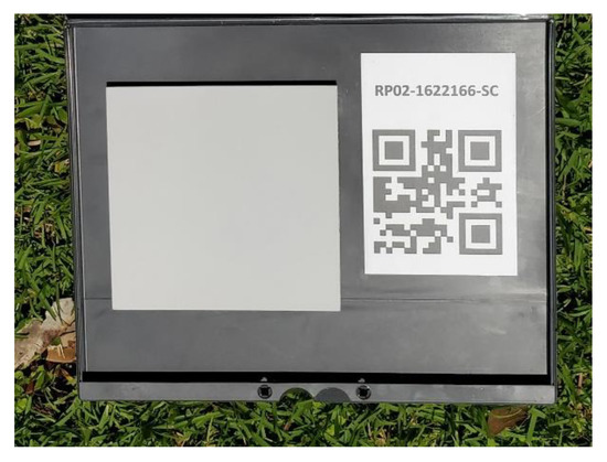
Figure 1.
Image of the calibrated reflectance panel, which was captured before each flight. Using the calibrated reflectance panel enabled more accurate compensation for incident light conditions and generation of quantitative data.
Table 2.
Imaging conditions, including acquisition dates, number of images, weather, and height of the drone.
Two different heights were explored for image acquisition, due to the small size of flower and fruit: one was at 2 m and the other was at three meters, as shown in Figure 2. The drone could take higher resolution images at 2 m, but only covered two rows in each image. On the other hand, at three meters, three rows could be covered but the plants had lower resolution in the images. In order to meet the 70% frontal overlap and 60% side overlap requirement for building orthoimages [43,44], the drone took an average of 185 images at 3 m, which took approximately 25 min for the whole field. At two meters, the drone took approximately 40 min for the whole field, with an average of 479 images. All the flights were performed automatically by the DJI Ground Station Pro (DJI Technology Co., Ltd., Shenzhen, China) iPad application, which is designed to conduct automated flight missions and manage the flight data of DJI drones [45]. The three-meter height images were taken in March 2018 and two-meter height images were taken from April to early June in 2018. Another three sets of two-meter images were acquired in November and December 2018, during the following season, so we could evaluate the developed model on image sets acquired in a different season.
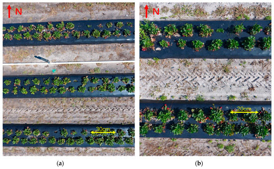
Figure 2.
Two heights were chosen for the image acquisition: (a) at a three-meter height, three rows were acquired in a single image; and (b) at a two-meter height, two rows were acquired in a single image.
2.2. Orthoimage Construction
In order to identify the exact numbers of flowers and strawberries in every square meter, orthoimages were needed. An orthoimage is a raster image created by stitching aerial photos which have been geometrically corrected for perspective, so that the photos do not have any distortion. An orthoimage can be used to measure true distances, because it is adjusted for topographic relief, lens distortion, and camera tilt, and can present the Earth’s surface accurately. With the help of orthoimages, we can locate the position of every flower and strawberry and build their distribution maps. The accuracy of the orthoimages was mainly based on the quality of the aerial images, which could be significantly affected by the camera resolution, focal length, and flight height. The ground sample distance (GSD) was the distance between pixel centers in the image measured on the ground, which can be used to measure the quality of aerial images and orthoimages, calculated with the formula:
where GSD is ground sample distance, H is flying height, c is camera focal length, and λ is camera sensor pixel size. For the 3 m height images, the GSD was 2.4 mm, and for the 2 m height images, the GSD was 1.6 mm. The process of building orthoimages is shown in Figure 3.
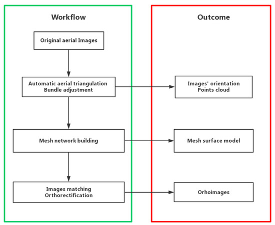
Figure 3.
Steps for generating orthoimages. An orthoimage is a raster image came from stitching aerial photos, and the process is a series of methods to make the orthoimage represent the same area and distance as in the real world.
Firstly, the aerial triangulation was processed to determine all image orientations and surface projections, with the help of GPS and position orientation system (POS) information provided by the drone, by using the pyramid matching strategy and bundle adjustment to match key points on each level of images [46]. Bundle adjustment [47] treats the measured area as a whole block and uses a least-squares method to meet the corresponding space intersection conditions, which can be explained by the following formula:
Assuming the image feature error is consistent with the Gaussian distribution, the number of 3D points is , and the number of images is, is the actual projected coordinates of point on the image. If point was visible on image ,; otherwise,. was the predicted projection coordinate of point point on image. The formula minimizes the projected error of 3D points onto the images and obtains more precise image orientations and 3D points.
After the point-cloud model was generated for the irregular distribution cloud data, mesh networks were needed to store and read the surface information of objects. An irregular mesh network, such as a triangulated irregular network (TIN) [48], was used to join discrete points into triangles that covered the entire area without overlapping with each other. Thus, it established a spatial relationship between discrete points. Using the Markov random field method [49], each mesh network matched the best suitable image as its model texture, based on the spatial positions and corresponding visible relationships.
The relationship of the x, y image co-ordinate to the real-world co-ordinate was calculated for orthorectification; that is, to remove the effects of image distortion caused by the sensor and viewing perspective. Similarly, a mathematical relationship between the ground co-ordinates, represented by the mesh model and the real-world co-ordinate, was computed and used to determine the proper position of each pixel from the source image to the orthoimage. The orthoimage’s distance and area are uniform in relationship to real-world measurements.
2.3. Date Pre-Processing
In order to identify objects in images using Faster R-CNN, the locations and classes of the objects need to be determined first. Faster R-CNN requires bounding box annotation for object localization and detection. Annotations of three different objects were collected using rectangular bounding boxes, as shown in Figure 4: flowers with white color, strawberries with red color, and immature strawberries with green or yellow color. All labels were created manually using the labelImg software developed by the Computer Science and Artificial Intelligence Laboratory (MIT, MA, USA).
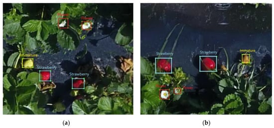
Figure 4.
Image label examples as (a,b). Three objects were chosen for classification: flowers with red bounding boxes, mature strawberries with blue bounding boxes, and immature fruit with yellow bounding boxes.
All the labeled images came from the orthoimages. The orthoimages were split into small rectangular images (480 × 380 pixels) to train the Faster R-CNN model faster. Every small image had its own sequence name, so it would be easy to restore the orthoimages from the small images after detection.
The images from March to early June were labeled for training the Faster R-CNN model; the total number was 12,526. Of these, 4568 were from the three-meter height image set and 7958 of them were from the two-meter height image set. Ten objects of interest were chosen for detection: flower at 2 m, flower at 3 m, Sensation strawberry at 2 m, Sensation strawberry at 3 m, Sensation immature at 2 m, Sensation immature at 3 m, Radiance strawberry at 2 m, Radiance strawberry at 3 m, Radiance immature at 2 m, and Radiance immature at 3 m. Five-fold cross-validation was used to train and test the model. In five-fold cross-validation, the original sample is randomly divided into five equal-size sub-samples. One of the five sub-samples was retained as the validation data for testing the model, and the remaining four sub-samples were used as training data. The cross-validation process was then repeated five times, with each of the five sub-samples being used exactly once as the validation data. Then, the results from the five iterations were averaged (or otherwise combined) to produce a single estimation. The advantage of this method was that all observations were used for both training and validation, and each observation was used for validation exactly once. The numbers of training and test images for each object are shown in Table 3. All the objects detected at the same height (for example, flower at 2 m, Sensation mature and immature fruit at 2 m, and Radiance mature and immature fruit at 2 m) shared the same image set.
Table 3.
Number of images of each object used for training and testing in five-fold cross-validation.
2.4. Model Training
We used the Faster R-CNN method based on the ResNet-50 architecture [50] in this study. As shown in Figure 5, instead of stacking layers directly to fit a desired underlying mapping, like VGG nets [51], ResNet-50 introduces a deep residual learning framework to fit a residual mapping which helps to address the degradation problem [52]. The deep residual learning framework is composed of a stack of residual blocks, each of which consists of a small network plus a skip connection. If an identification mapping is optimal, it is easier to push the residual to zero and skip the connection than to fit an identification mapping by a stack of non-linear layers. Compared with VGG-16/19, ResNet-50 has lower error rates for ImageNet validation and a lower complexity.
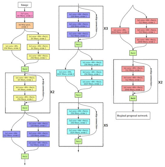
Figure 5.
ResNet-50, a 50-layer residual network which is used for the feature extraction in the Faster R-CNN architecture.
The whole structure of Faster R-CNN [36] is shown in Figure 6. It consists of convolutional layers (ResNet-50), region proposal networks (RPN), an ROI pooling layer, and a classifier. The convolutional layers were used for extracting image features to be shared with the RPN and classifier. The feature maps were first operated on by a 3 × 3 convolution layer. Then region proposals were generated in the RPN by classifying the feature vectors for each region with the softmax function and locating the boundary with bounding box regression. The proposals generated from RPN had different shapes, which could not be operated on by full connection and, so, the ROI pooling collects the features and proposals from former layers and filters the max values to the classifier. The classifier then determines if the region belongs to an object class of interest. Compared with R-CNN [32] or Fast R-CNN [37], the RPN of Faster R-CNN shares convolutional features with the classification network, where the two networks are concatenated as one network which can be trained and tested through an end-to-end process. This architecture makes the running time for region proposal generation much shorter. The model was trained on ImageNet and fine-tuned by initializing a new classification layer and updating all layers for both the region proposal and classification networks. This process is named transfer learning. The training iteration was 5000, with a basic learning rate of 0.01.
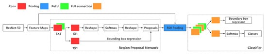
Figure 6.
Faster R-CNN is a single, unified network for object detection. The region proposal network (RPN) shares convolutional features with the classification network, where the two networks are concatenated as one network that can be trained and tested through an end-to-end process, which makes the running time for region proposal generation much shorter.
The orthoimage and Faster R-CNN processes were performed on the image dataset with a desktop computer consisting of an NVIDIA TITAN X (Pascal) integrated RAMDAC 12 GB graphics card (NVIDIA, Santa Clara, USA) and Intel Core (TM) i7-4790 CPU 4.00 GHz (Intel, Santa Clara, USA). The algorithms were performed in TensorFlow on the Windows 7 operating system.
3. Results
3.1. Orthoimages Generation
We used the Pix4D software to generate high-resolution orthoimages. As the two-meter height image sets had more images, their point cloud models were more dense and complete. The mesh surface models were established based on the point cloud, as shown in Figure 7. The image shown in Figure 8 was the final orthoimage from the mesh surface models, a 2D projection of the 3D model. The upper three rows in the orthoimages contained the Sensation variety and the other two rows were Radiance. There was some distortion at the edges of the orthoimages, due to the lack of image overlap. However, this did not affect the counting of the number of flowers and strawberries.
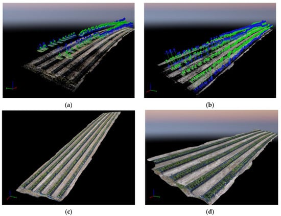
Figure 7.
The point cloud model and mesh surface results: (a) the point clouds model of the 3 m height image set; (b) the point cloud model of the 2 m height image set; (c) the mesh surface model of the 3 m height image set; and (d) the mesh surface model of the 2 m height image set.
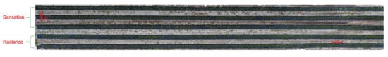
Figure 8.
Final orthoimage. The upper three rows (in the north direction) contained the Sensation variety and the lower two rows were Radiance.
3.2. Faster R-CNN Detection Presults
Both quantitative and qualitative measurements were taken to evaluate the performance of Faster R-CNN detection in three experimental settings: (1) we trained the Faster R-CNN model on the image sets from March to early June 2018, and analyzed its performance; (2) we compared the Faster R-CNN detection results of 2 m images and 3 m images; and (3) we used the Faster R-CNN model trained on the image sets from March to early June to count flower numbers using the image sets from November to December 2018. The deep learning counting results were compared with the manual count to check the deep learning counting accuracy and calculate flower occlusion.
3.2.1. Quantitative Analysis of Faster R-CNN Detection Performance
The correctness of a detected object is evaluated by the intersection-over-union (IoU) overlap with the corresponding ground truth bounding box. The IoU overlap was defined as follows:
where Area(GroundTruthI Detected) is the intersection area of the prediction and ground truth bounding boxes and the Area(GroundTruthU Detected) is the union area of the prediction and ground truth bounding boxes. It was considered to be a true positive (TP) if the IoU was greater than the threshold value. If a detected object did not match with the ground truth bounding box, it was considered to be a false positive (FP). A false negative (FN) was determined if the ground truth bounding box was missed. We chose 0.5 for the threshold value, which means if the IoU between the prediction and ground truth bounding boxes was greater than 0.5, it was considered to be a TP. This was the same as in the ImageNet challenge.
Precision and recall are calculated according to the following equations:
The single class detection performance was measured with average precision (AP), which is the area under the precision–recall curve [53]. The overall detection performance was measured with the mean average precision (mAP) score, which is the average AP value over all classes. The higher the mAP was, the better the overall detection performance of the Faster R-CNN. The detection performance of the Faster R-CNN is shown in Table 4.
Table 4.
The Faster R-CNN detection performance for each object.
As we can see from Table 4, the detection performance on the 2 m image set increased significantly, from that of the 3 m one, for the detection of flowers, immature fruit, and mature fruit. The best detection results were Radiance strawberry mature fruit at 2 m (94.5%), Sensation mature fruit at 2 m (86.4%), and flowers (from both varieties) at 2 m (87.9%). The worst results were Radiance immature fruit at 3 m (70.2%), flowers (from both varieties) at 3 m (77.5%), and Sensation immature fruit at 3 m (74.2%). The mature fruit detection performances were much better than that of the immature fruit, but the gap was decreased at 2 m. The total mAP was 0.83 for all 2 m objects and 0.72 for all 3 m objects.
3.2.2. Qualitative Analysis for Different Heights’ Detection Results
The small (480 × 380 pixel) images were stitched back into the original orthoimages after Faster R-CNN detection. Figure 9 shows orthoimage detection examples at two-meter and three-meter heights. There were some blurred parts, which were caused by the strong wind produced by the propellers of the drone. The strong wind could help the camera capture more flowers and fruits hidden under the leaves but also caused the strawberry plants to slightly shake when the drone was flying close to the ground. This may affect the quality of aerial images for orthoimage building. The leaves were more susceptible to wind than flowers and strawberries, so most of the blurred or distorted parts were in the leaves, rather than the flowers or fruits, which barely affected the detection results. This phenomenon was more common in 2 m height orthoimages, as the drone flew closer to the ground. In both images, the model detected flowers precisely, even though some of them were covered partially by leaves. However, in both images, the model confused some mature and immature strawberries with dead leaves. At 3 m height, there were more false detections for mature and immature fruit than at 2 m heights.
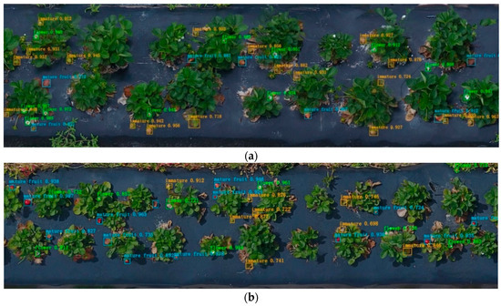
Figure 9.
Faster R-CNN detection examples at (a) 2 m and (b) 3 m heights. The 3 m height orthoimage has lower resolution than that at 2 m height. The detection results for the flowers and mature fruit were more precise than those of the immature fruit. The model could discover flowers, even when part of the petal was hidden by leaves. However, the model confused immature fruit with green leaves and mature fruit with dead leaves in some areas.
In order to check the effect of different heights on detection performance, we compared the detection results between 2 m and 3 m split orthoimages. Figure 10 and Figure 11 show some quantitative results for 2 m and 3 m split orthoimages.
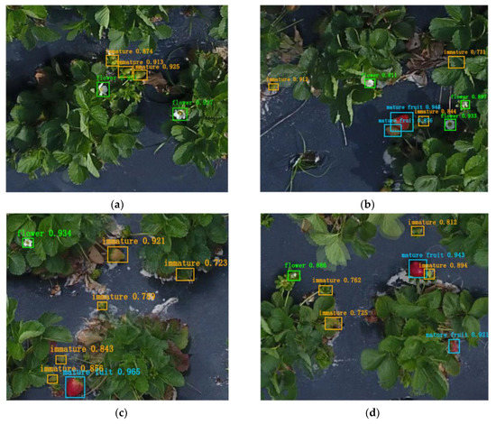
Figure 10.
Detection results for 2 m split orthoimages: (a,b) are examples of Sensation; (c,d) are examples of Radiance.
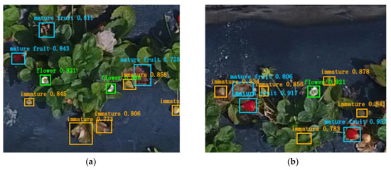
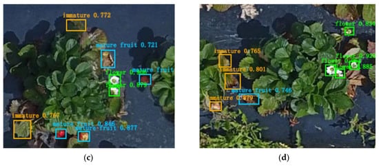
Figure 11.
Detection results for 3 m split orthoimages: (a,b) are examples of Sensation; (c,d) are examples of Radiance.
We can see that the 2 m images were clearer and more precise than the 3 m images at the same scale level. The 3 m images had more blur and distortion problems. Therefore, there were many more FP for mature and immature fruit in the 3 m images than the 2 m ones.
3.2.3. Comparison of Deep Learning Count and Manual Count
We used the Faster R-CNN model, trained by the images from March to early June, to count the flower numbers in the images from November and December 2018. We manually counted the number of flowers in the field before flying the drone to capture images, so that the manual count could be compared with the deep learning count. For each bounding box prediction, the neural network also output a confidence (between 0 and 1), indicating how likely it was that the proposed box contained the correct object. A threshold was used to remove all predictions that had a confidence below the threshold. By increasing the confidence threshold, fewer predictions are kept and, therefore, recall decreases, but precision should increase. Alternatively, decreasing the threshold will improve recall while potentially decreasing precision. Higher values of precision and recall are preferable, but they are typically inversely related. Thus, the score threshold should be properly adjusted, depending on the circumstances and applications. In this study, we set the confidence threshold as 0.85 for the deep learning counting, because we noted that most FP in flower detection had a relatively low confidence (lower than 0.85), whereas objects being truly detected were all above 0.85.
Although the wind generated by the drone propeller could expose some of the flowers hidden under the leaves, there were still some flowers hidden under the leaves which could not be captured by the flight images. Thus, the effect of occlusion needed to be considered when using the deep learning model to count the flowers. Occlusion and deep learning count accuracy are calculated according to the following equations:
Table 5 shows the comparison results between manual count and deep learning count in the number of flowers. The average accuracy for deep learning counting is 84.1%, and average occlusion is 13.5%. We can see that the occlusion and FN number increased as the number of flowers decreased. Generally, when the flowers in the field are the majority, the proportion of the mature and immature fruit is relatively smaller, which will lead to a burst growth of the fruit and the majority will turn to (mature and immature) fruit. Thus, a decrease in the number of flowers means that more flowers become immature or mature fruit and that the leaves would grow larger to feed the fruit, which leads to an increase of occlusion, making the flowers harder detect.
Table 5.
Comparison between manual count and deep learning count of the number of flowers.
3.3. Comparison of Region-Based Object Detection Methods
Region-based CNN frameworks have been commonly used in the area of object detection. In this section, we compare the detection performance of Faster R-CNN with other region-based object detection methods, including R-CNN [32] and Fast R-CNN [37]. These detection models are based on the same architecture (ResNet-50) and were trained on the same strawberry dataset. We used selective search (SS) to extract 2000 region proposals for the R-CNN and Fast R-CNN models and RPN to generate 400 proposals for the Faster R-CNN model [36]. The results are shown in Table 6.
Table 6.
Comparison between different region-based object detection methods.
As summarized in Table 6, Faster R-CNN could perform 8.872 frames per second (FPS), in terms of detection rate; much faster than the R-CNN and Fast R-CNN methods. The Faster R-CNN method also had the highest mAP score (0.772) and the lowest training time (5.5 h). It is clear that the performance of the Faster R-CNN model exceeded those of the R-CNN and Fast R-CNN models.
3.4. Flower and Fruit Distribution Map Generation
It usually takes only a few weeks for flowers to become fruit for both Sensation and Radiance varieties. In order to observe the growth cycle of strawberry fields, we built distribution maps of flowers and immature fruit on 13 April and immature and mature fruit on 27 April, based on the numbers and locations calculated by Faster R-CNN. The numbers of flowers, mature fruit, and immature fruit (including both TP and FP) detected by Faster R-CNN on 13 April and 27 April are shown in Table 7.
Table 7.
Number of flowers, mature fruit, and immature fruit counted by the Faster R-CNN.
Flower and fruit distribution maps were created by ArcMap 10.3.1 (ESRI, Redlands, USA). Inverse distance weighting (IDW) was used as an interpolation method. The field was divided into 30 areas (each row was divided into six areas) and the numbers of flowers, mature fruit, and immature fruit of each area were counted and placed at the center point of each area. For the IDW, the variable search radius was 10 points and the power was 2. Distribution maps of flowers on 13 April and immature fruit on 27 April are shown in Figure 12.
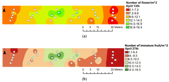
Figure 12.
Distribution map based on the inverse distance weighting (IDW) interpolation: (a) flower map for 13 April; and (b) immature fruit map for 27 April.
By comparing these two maps, we can see that the distribution of flowers on 13 April had many similarities to the distribution of immature fruit on 27 April. Both had high production in the central part of the field and have relatively low production in the east and west edges, which means most flowers became immature fruit after two weeks.
Both flowers and immature fruit on 13 April could become mature fruit on 27 April, so we compared them in Figure 13.
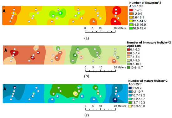
Figure 13.
Comparison of flower and immature fruit maps on 13 April with the mature fruit map on 27 April: (a) flower map on 13 April; (b) immature fruit map on 13 April; and (c) mature fruit map on 27 April.
We can see that the mature fruit map of 27 April shows a similar trend to both the flower map of 13 April and the immature fruit map of 13 April. For the west part, the mature fruit map is more similar to the immature map; on the other hand, the east part is more similar to the flower map. The central part of the mature fruit map is more likely a combination of the flower and immature fruit maps. Thus, both the flowers and immature fruit on 13 April contributed to the mature fruit distribution on 27 April.
4. Discussion
In order to quickly count and locate flowers and fruit in the strawberry field with the help of a normal consumer drone, we stitched the images captured by the drone together and transformed them to an orthoimage. An orthoimage is a raster image that has been geometrically corrected for topographic relief, lens distortion, and camera tilt, which accurately presents the Earth’s surface and can be used to measure true distance [18,54]. The quality of orthoimages mainly depends on the quality and overlaps of aerial images. The frontal overlap is usually 70–80% and the side overlap is usually no less than 60%. For the same overlap conditions, the closer the aircraft is to the ground, the higher the GSD of the images will be, which helps the detection system to perform better. However, it will also take more time and consume more battery power to take images at a lower altitude, which would reduce efficiency and drone life. The specific working altitude should be adjusted according to the environmental conditions and task requirements. Many studies [25,44,55,56] set the frontal overlap around 80% and 70% for the side overlap. Most of their drones flew above 50 m in height and had relatively low GSD values. In our experiments, the flight images were taken near the ground, so we set the frontal overlap to be 70% and the side overlap to 60%, in order to increase flight efficiency while ensuring the orthoimage building requirements.
Some distortions happened at the edges of the orthoimages, due to the lack of image overlap. More flight routes will be used to cover the field edge in our next experiment. There were also some blurred or distorted parts in the plant areas of the orthoimages. These were caused by the strong wind produced by the drone as it flew across the field. These were more common in 2-m height orthoimages, as the drone flew closer to ground. Most of the blurred or distorted parts happened in the leaf areas, which were more susceptible to wind than flowers and fruits; the flowers and fruits were barely affected. As a bonus, the wind could actually help the camera to capture more flowers and fruit hidden under the leaves, so more flowers and fruit were detected in the 2 m height orthoimages.
Object detection is the task of finding different objects in an image and classifying them. R-CNN [32] was the first region-based object detection method. It selects multiple high-quality proposed regions by using the selective search [33] method and labels the category and ground-truth bounding box of each proposed region. Then, a pre-trained CNN transforms each proposed region into the input dimensions required by the network and uses forward computation to output the feature vector extracted from the proposed regions. Finally, the feature vectors are sent to linear support vector machines (SVMs) for object classification and then to a regressor to adjust the detection position. Fast R-CNN [37] inherited the framework of R-CNN, but performs CNN forward computation on the image as a whole and uses a region-of-interest pooling layer to obtain fixed-size feature maps. Faster R-CNN replaced the selective search method with a region proposal network. This reduces the number of proposed regions generated, while ensuring precise object detection. We compared the performances of R-CNN, Fast R-CNN, and Faster R-CNN on our dataset. The results showed that Faster R-CNN had the lowest training time, highest mAP score, and the fastest detection rate. So far, Faster R-CNN is the best region-based object detection method for identifying different objects and their boundaries in images.
In our detection system, we fine-tuned a Faster R-CNN detection network which was based on the pre-trained ImageNet model which gave state-of-the-art performance on split orthoimage data. The average precisions varied from 0.76 to 0.91 for the 2 m images and from 0.61 to 0.83 for the 3 m images. Detection for flowers and mature fruit worked well, but immature fruit detection did not meet our expectations. The shapes and colors of immature fruit were sometimes very similar to dead leaves, which was the main reason for the poor results. More images are needed for the future network training. Additionally, there were always some occlusion problems, where flowers and fruit hidden under the leaves could not be captured by the camera. This occlusion varied slightly in the different growth stages of strawberries; when more flowers turned to fruit, the leaves tended to expand larger in order to deliver more nutrients to the fruit. The occlusion was around 11.5% and 15.2% in our field in November and December 2018, respectively. Further field experiments are needed to identify different seasonal occlusions, so that we can establish an offset factor to reduce counting errors by deep learning detection.
We chose IDW for the interpolation of the distribution maps. IDW is a method of interpolation that estimates cell values by averaging the values of sample data points in the neighborhood of each processing cell. The closer a point is to the center of the cell being estimated, the more influence (or weight) it has in the averaging process. Kriging is an advanced geostatistical procedure that generates an estimated surface from a scattered set of points with z-values; however, it requires many more data points. A thorough investigation of the spatial behavior of the phenomenon represented by the z-values should be done before selecting the best interpolation method for generating the output surface. In many studies, Kriging interpolation has been reported to perform better than IDW. However, this is highly dependent on the variability in the data, distance between the data points, and number of data points available in the study area. We will try both methods with more data in the future, and better results may be obtained by comparing multiple interpolation results with actual counts in the field and acquired images.
5. Conclusions
In this paper, we presented a deep learning strawberry flower and fruit detection system, based on high resolution orthoimages reconstructed from drone images. The system could be used to build yield estimation maps, which could help farmers predict the weekly yields of strawberries and monitor the outcome of each area, in order to save their time and labor costs.
In developing this system, we used a small UAV to take near-ground RGB images for building orthoimages at 2 m and 3 m heights, where the GSD was 2.4 mm and 1.6 mm, respectively. After their generation, we split the original orthoimages into sequential pieces for Faster R-CNN detection, which was based on the ResNet-50 architecture and transfer learning from ImageNet, to detect 10 objects. The results were presented in both a quantitative and qualitative way. The best detection performance was for mature fruit of the Sensation variety at 2 m, with an AP of 0.91. Immature fruit of the Radiance variety at 3 m was the most difficult to detect (since the model tended to confuse them with green leaves), having the worst AP of 0.61. We also compared the number of flowers counted by the deep learning model and the manual count numbers, and found the average deep learning counting accuracy to be 84.1%, with an average occlusion of 13.5%. Thus, this method has proved that it can be used to count flower numbers effectively.
We also tried to build distribution maps of flowers and immature fruit on 13 April and immature and mature fruit on 27 April, based on the numbers and distributions calculated by Faster R-CNN. The results showed that the mature fruit map of 27 April had obvious connection with the flower and immature fruit maps of 13 April. The flower distribution map of 13 April and immature map of 27 April also showed a strong relationship, which proved that this system could help farmers to monitor the growth of strawberry plants.
Author Contributions
Conceptualization: Y.C. and W.S.L.; data curation: Y.C. and H.G.; formal analysis: Y.C.; funding acquisition: W.S.L. and Y.H.; methodology: Y.C., W.S.L., Y.Z., and Y.H.; resources: N.P. and Y.Z.; software: Y.C.; supervision: W.S.L. and Y.H.; validation: W.S.L., H.G., C.F., and Y.H.; visualization: Y.C.; writing—original draft, Y.C.; writing—review and editing: Y.C., W.S.L., H.G., C.F., and Y.H.
Funding
The main author was supported by China Scholarship Council. This research was funded by Florida Strawberry Research Education Foundation, Inc. (FEREF), and Florida Foundation Seed Producers, Inc. (FFSP).
Acknowledgments
The authors would like to thank Ping Lin and Chao Li for their assistance in this study.
Conflicts of Interest
The authors declare no conflict of interest.
References
- USDA-NASS 2018 State Agriculture Overview. Available online: https://www.nass.usda.gov/Quick_Stats/Ag_Overview/stateOverview.php?state=FLORIDA (accessed on 26 March 2019).
- Taylor, P.; Savini, G.; Neri, D.; Zucconi, F.; Sugiyama, N. Strawberry Growth and Flowering: An Architectural Model. Int. J. Fruit Sci. 2008, 5, 29–50. [Google Scholar]
- Chandler, C.K.; Albregts, E.E.; Howard, C.M.; Dale, A. Influence of Propagation Site on the Fruiting of Three Strawberry Clones Grown in a Florida Winter Production System. Proc. Fla. State Hortic. Soc. 1989, 102, 310–312. [Google Scholar]
- Chercuitte, L.; SulIivan, J.A.; Desjardins, Y.D.; Bedard, R. Yield Potential and Vegetative Growth of Summer-planted Strawberry. J. Am. Soc. Hortic. Sci. 2019, 116, 930–936. [Google Scholar] [CrossRef]
- Kadir, S.; Sidhu, G.; Al-Khatib, K. Strawberry (Fragaria xananassa Duch.) growth and productivity as affected by temperature. HortScience 2006, 41, 1423–1430. [Google Scholar] [CrossRef]
- Chandler, C.K.; Mackenzie, S.J.; Herrington, M. Fruit Development Period in Strawberry Differs Among Cultivars, and Is Negatively Correlated With Average Post Bloom Air Temperature. Proc. Fla. State Hortic. Soc. 2004, 117, 83–85. [Google Scholar]
- Wang, S.Y.; Zheng, W. Effect of plant growth temperature on antioxidant capacity in strawberry. J. Agric. Food Chem. 2001, 49, 4977–4982. [Google Scholar] [CrossRef] [PubMed]
- Paroussi, G.; Voyiatzis, D.G.; Paroussis, E.; Drogoudi, P.D. Growth, flowering and yield responses to GA3 of strawberry grown under different environmental conditions. Sci. Hortic. (Amst.) 2002, 96, 103–113. [Google Scholar] [CrossRef]
- Abdel-Mawgoud, A.M.R.; Tantawy, A.S.; El-Nemr, M.A.; Sassine, Y.N. Growth and Yield Responses of Strawberry Plants to Chitosan Application. Eur. J. Sci. Res. 2010, 39, 161–168. [Google Scholar]
- Kerfs, J.; Eagan, Z.; Liu, B. Machine Vision for Strawberry Detection. In Proceedings of the 2017 Annual International Meeting ASABE, Washington, DC, USA, 16–19 July 2017. [Google Scholar]
- Olam, H. Photoperiod and temperature interactions in growth and flowering of strawberry. Physiol. Plant. 1977, 40, 21–26. [Google Scholar]
- Døving, A.; Måge, F. Prediction of Strawberry Fruit Yield. Acta Agric. Scand. Sect. B Soil Plant Sci. 2001, 51, 35–42. [Google Scholar] [CrossRef]
- Døving, A.; Måge, F. Prediction of the strawberry season in Norway. Acta Agric. Scand. Sect. B Soil Plant Sci. 2001, 51, 28–34. [Google Scholar] [CrossRef]
- Sønsteby, A.; Karhu, S. Strawberry production, growth and development in northern climates. Int. J. Fruit Sci. 2005, 5, 107–114. [Google Scholar] [CrossRef]
- Misaghi, F.; Mohammadi, K.; Limited, O.E.; Ehsani, R. Application of Artificial Neural Network and Geostatistical Methods in Analyzing Strawberry Yield Data. In Proceedings of the 2004 ASAE Annual Meeting, Kyoto, Japan, 7–8 October 2004; American Society of Agricultural and Biological Engineers: St. Joseph, MI, USA, 2004; p. 1. [Google Scholar]
- MacKenzie, S.J.; Chandler, C.K. A method to predict weekly strawberry fruit yields from extended season production systems. Agron. J. 2009, 101, 278–287. [Google Scholar] [CrossRef]
- Everaerts, J. The use of unmanned aerial vehicle (UAVS) for remote sensing and mapping. Remote Sens. Spat. Inf. Sci. 2008, 38, 1187–1192. [Google Scholar]
- Candiago, S.; Remondino, F.; De Giglio, M.; Dubbini, M.; Gattelli, M. Evaluating multispectral images and vegetation indices for precision farming applications from UAV images. Remote Sens. 2015, 7, 4026–4047. [Google Scholar] [CrossRef]
- Garcia-Ruiz, F.; Sankaran, S.; Maja, J.M.; Lee, W.S.; Rasmussen, J.; Ehsani, R. Comparison of two aerial imaging platforms for identification of Huanglongbing-infected citrus trees. Comput. Electron. Agric. 2013, 91, 106–115. [Google Scholar] [CrossRef]
- Baluja, J.; Diago, M.P.; Balda, P.; Zorer, R.; Meggio, F.; Morales, F.; Tardaguila, J. Assessment of vineyard water status variability by thermal and multispectral imagery using an unmanned aerial vehicle (UAV). Irrig. Sci. 2012, 30, 511–522. [Google Scholar] [CrossRef]
- Zarco-Tejada, P.J.; Guillén-Climent, M.L.; Hernández-Clemente, R.; Catalina, A.; González, M.R.; Martín, P. Estimating leaf carotenoid content in vineyards using high resolution hyperspectral imagery acquired from an unmanned aerial vehicle (UAV). Agric. For. Meteorol. 2013, 171–172, 281–294. [Google Scholar] [CrossRef]
- Zahawi, R.A.; Dandois, J.P.; Holl, K.D.; Nadwodny, D.; Reid, J.L.; Ellis, E.C. Using lightweight unmanned aerial vehicles to monitor tropical forest recovery. Biol. Conserv. 2015, 186, 287–295. [Google Scholar] [CrossRef]
- Zhang, Y.; Xiao, Y.; Zhuang, Z.; Zhou, L.; Liu, F.; He, Y. Development of a near ground remote sensing system. Sensors (Switz.) 2016, 16, 648. [Google Scholar] [CrossRef]
- Sagan, V.; Maimaitijiang, M.; Sidike, P.; Eblimit, K.; Peterson, K.T.; Hartling, S.; Esposito, F.; Khanal, K.; Newcomb, M.; Pauli, D.; et al. UAV-based high resolution thermal imaging for vegetation monitoring, and plant phenotyping using ICI 8640 P, FLIR Vue Pro R 640, and thermomap cameras. Remote Sens. 2019, 11, 330. [Google Scholar] [CrossRef]
- Torres-Sánchez, J.; López-Granados, F.; De Castro, A.I.; Peña-Barragán, J.M. Configuration and Specifications of an Unmanned Aerial Vehicle (UAV) for Early Site Specific Weed Management. PLoS ONE 2013, 8. [Google Scholar] [CrossRef] [PubMed]
- Xiang, H.; Tian, L. Development of a low-cost agricultural remote sensing system based on an autonomous unmanned aerial vehicle (UAV). Biosyst. Eng. 2011, 108, 174–190. [Google Scholar] [CrossRef]
- Behmann, J.; Mahlein, A.K.; Rumpf, T.; Römer, C.; Plümer, L. A review of advanced machine learning methods for the detection of biotic stress in precision crop protection. Precis. Agric. 2015, 16, 239–260. [Google Scholar] [CrossRef]
- Choi, D.; Lee, W.S.; Ehsani, R.; Schueller, J.; Roka, F.M. Detection of dropped citrus fruit on the ground and evaluation of decay stages in varying illumination conditions. Comput. Electron. Agric. 2016, 127, 109–119. [Google Scholar] [CrossRef]
- Andrejko, E.; Valley, S. Deep Learning in Agriculture. Comput. Electron. Agric. 2018, 147, 70–90. [Google Scholar]
- Dyrmann, M.; Karstoft, H.; Midtiby, H.S. Plant species classification using deep convolutional neural network. Biosyst. Eng. 2016, 151, 72–80. [Google Scholar] [CrossRef]
- Dairi, A.; Harrou, F.; Senouci, M.; Sun, Y. Unsupervised obstacle detection in driving environments using deep-learning-based stereovision. Robot. Auton. Syst. 2018, 100, 287–301. [Google Scholar] [CrossRef]
- Girshick, R.; Donahue, J.; Darrell, T.; Malik, J. Rich feature hierarchies for accurate object detection and semantic segmentation. In Proceedings of the IEEE Conference on Computer Vision and Pattern Recognition, Columbus, OH, USA, 23–28 June 2014; pp. 580–587. [Google Scholar]
- Uijlings, J.R.R.; Van De Sande, K.E.A.; Gevers, T.; Smeulders, A.W.M. Selective search for object recognition. Int. J. Comput. Vis. 2013, 104, 154–171. [Google Scholar] [CrossRef]
- Zitnick, C.L.; Dollár, P. Edge boxes: Locating object proposals from edges. In Proceedings of the 13th European Conference, Zurich, Switzerland, 6–12 September 2014; Springer: Berlin, Germany, 2014; pp. 391–405. [Google Scholar]
- Christiansen, P.; Nielsen, L.N.; Steen, K.A.; Jørgensen, R.N.; Karstoft, H. DeepAnomaly: Combining background subtraction and deep learning for detecting obstacles and anomalies in an agricultural field. Sensors (Switz.) 2016, 16, 1904. [Google Scholar] [CrossRef]
- Ren, S.; He, K.; Girshick, R.; Sun, J. Faster R-CNN: Towards Real-Time Object Detection with region proposal networks. IEEE Trans. Pattern Anal. Mach. Intell. 2017, 39, 1137–1149. [Google Scholar] [CrossRef] [PubMed]
- Girshick, R. Fast R-CNN. In Proceedings of the 2015 IEEE International Conference on Computer Vision (ICCV), Washington, DC, USA, 7–13 December 2015; pp. 1440–1448. [Google Scholar]
- Bargoti, S.; Underwood, J. Deep fruit detection in orchards. In Proceedings of the 2017 IEEE International Conference on Robotics and Automation (ICRA), Singapore, 29 May–3 June 2017; pp. 3626–3633. [Google Scholar]
- Baweja, H.S.; Parhar, T.; Mirbod, O.; Nuske, S. StalkNet: A Deep Learning Pipeline for High-Throughput Measurement of Plant Stalk Count and Stalk Width. Field Serv. Robot. 2018, 5, 271–284. [Google Scholar]
- Sa, I.; Ge, Z.; Dayoub, F.; Upcroft, B.; Perez, T.; McCool, C. Deepfruits: A fruit detection system using deep neural networks. Sensors 2016, 16, 1222. [Google Scholar] [CrossRef] [PubMed]
- Florida Department of Agriculture and Consumer Services Florida Crops Seasonal Availability/Typical Harvest Times. Available online: https://www.freshfromflorida.com/Consumer-Resources/Buy-Fresh-From-Florida/Crops-in-Season (accessed on 21 December 2018).
- Radiometric Corrections. Available online: https://support.pix4d.com/hc/en-us/articles/202559 (accessed on 11 September 2018).
- Dandois, J.P.; Olano, M.; Ellis, E.C. Optimal altitude, overlap, and weather conditions for computer vision uav estimates of forest structure. Remote Sens. 2015, 7, 13895–13920. [Google Scholar] [CrossRef]
- Gonçalves, J.A.; Henriques, R. UAV photogrammetry for topographic monitoring of coastal areas. ISPRS J. Photogramm. Remote Sens. 2015, 104, 101–111. [Google Scholar] [CrossRef]
- DJI GS PRO. Available online: https://www.dji.com/hk-en/ground-station-pro (accessed on 15 March 2019).
- Snavely, N. Scene Reconstruction and Visualization from Internet Photo Collections: A Survey. IPSJ Trans. Comput. Vis. Appl. 2011, 3, 44–66. [Google Scholar] [CrossRef]
- Triggs, B.; Mclauchlan, P.; Hartley, R.; Fitzgibbon, A.; Triggs, B.; Mclauchlan, P.; Hartley, R.; Fitzgibbon, A.; Ajustment, B.; Triggs, S.B.; et al. Bundle Ajustment—A Modern Synthesis. In Proceedings of the International Workshop on Vision Algorithms, London, UK, 21–22 September 1999; Springer: Berlin/Heidelberg, Germany, 1999; pp. 298–372. [Google Scholar]
- Tucker, G.E.; Lancaster, S.T.; Gasparini, N.M.; Bras, R.L.; Rybarczyk, S.M. An object-oriented framework for distributed hydrologic and geomorphic modeling using triangulated irregular networks. Comput. Geosci. 2001, 27, 959–973. [Google Scholar] [CrossRef]
- Li, S.Z. Markov random field models in computer vision. In Proceedings of the 3rd European Conference on Computer Vision, Stockholm, Sweden, 2–6 May 1994; Springer: Berlin/Heidelberg, Germany, 1994; pp. 361–370. [Google Scholar]
- He, K.; Zhang, X.; Ren, S.; Sun, J. Deep residual learning for image recognition. In Proceedings of the 2016 IEEE Conference on Computer Vision and Pattern Recognition (CVPR), Las Vegas, NV, USA, 26 June–1 July 2016; pp. 770–778. [Google Scholar]
- Simonyan, K.; Zisserman, A. Very Deep Convolutional Networks for Large-Scale Image Recognition. arXiv 2014, arXiv:1409.1556. [Google Scholar]
- He, K. Convolutional Neural Networks at Constrained Time Cost. In Proceedings of the 28th IEEE Conference on Computer Vision and Pattern Recognition, Boston, MA, USA, 7–12 June 2015; pp. 5353–5360. [Google Scholar]
- Henderson, P.; Ferrari, V. End-to-end training of object class detectors for mean average precision. In Proceedings of the 13th Asian Conference on Computer Vision, Taibei, Taiwan, 20–24 November 2016; Springer: Berlin, Germany, 2016; pp. 198–213. [Google Scholar]
- Barrette, J.; August, P.; Golet, F. Accuracy assessment of wetland boundary delineation using aerial photography and digital orthophotography. Photogramm. Eng. Remote Sens. 2000, 66, 409–416. [Google Scholar]
- Brenner, C. Use of DTMs/DSMs and Orthoimages to Support Building Extraction. In Automatic Extraction of Man-Made Objects from Aerial and Space Images; Birkhäuser: Basel, Switzerland, 2010; pp. 169–212. [Google Scholar]
- Zarco-Tejada, P.J.; Diaz-Varela, R.; Angileri, V.; Loudjani, P. Tree height quantification using very high resolution imagery acquired from an unmanned aerial vehicle (UAV) and automatic 3D photo-reconstruction methods. Eur. J. Agron. 2014, 55, 89–99. [Google Scholar] [CrossRef]
© 2019 by the authors. Licensee MDPI, Basel, Switzerland. This article is an open access article distributed under the terms and conditions of the Creative Commons Attribution (CC BY) license (http://creativecommons.org/licenses/by/4.0/).