Abstract
True-color three-dimensional (3D) imaging exploits spatial and spectral information and can enable accurate feature extraction and object classification. The existing methods, however, are limited by data collection mechanisms when realizing true-color 3D imaging. We overcome this problem and present a novel true-color 3D imaging method based on a 32-channel hyperspectral LiDAR (HSL) covering a 431–751 nm spectral range. We conducted two experiments, one with nine-color card papers and the other with seven different colored objects. We used the former to investigate the effect of true-color 3D imaging and determine the optimal spectral bands for compositing true-color, and the latter to explore the classification potential based on the true-color feature using polynomial support vector machine (SVM) and Gaussian naive Bayes (NB) classifiers. Since using all bands of HSL will cause color distortions, the optimal spectral band combination for better compositing the true-color were selected by principal component analysis (PCA) and spectral correlation measure (SCM); PCA emphasizes the amount of information in band combinations, while SCM focuses on correlation between bands. The results show that the true-color 3D imaging can be realized based on HSL measurements, and three spectral bands of 466, 546, and 626 nm were determined. Comparing reflectance of the three selected bands, the overall classification accuracy of seven different colored objects was improved by 14.6% and 8.25% based on SVM and NB, respectively, classifiers after converting spectral intensities into true-color information. Overall, this study demonstrated the potential of HSL system in retrieving true-color and facilitating target recognition, and can serve as a guide in developing future three-channel or multi-channel true-color LiDAR.
1. Introduction
Target imaging has attracted significant research attention in remote sensing, and widely employs in resource exploration, agriculture, and forestry management [1,2,3]. Target imaging can be realized using spatial and spectral information, acquired by various types of sensors [4,5,6], and can realize non-destructive measurement of physiological processes of a target in a non-contact manner [7]. Target imaging also allows repeated observations, thus making it possible to detect in real-time, and reduce time and cost. The ultimate goal of imaging is to fully understand and classify detected objects based on information acquired from a target. With the continuous development of remote sensing technologies, imaging methods have become diversified [8,9].
The spectral imaging has been realized by passive multispectral/hyperspectral techniques, and is employed in medicine, agriculture and management of natural resources [10,11,12]. However, passive multispectral/hyperspectral imaging lacks information on the vertical dimension, which is essential in estimating old-growth forest canopy and vegetation biomass [13,14]. Laser scanning enables 3D imaging, yet it lacks the ability to acquire the spectral information, which is significant for bio-chemical parameter detection of plants [15]. To combine the strengths of both passive and active sensors, researchers have attempted to fuse point clouds and images [16,17]. Nonetheless, these methods face significant spatial and temporal registration problems due to the variation in detection mechanisms [18]. As a result, in recent years, multispectral/hyperspectral LiDAR (MSL/HSL) systems were developed; some even have been commercialized such as the Optech Titan system [19,20,21,22]. However, current MSL/HSL data application research mainly focuses on the inversion of vegetation biochemical parameters and target classification [23,24,25]. False-color 3D imaging has been realized based on MSL data [26], but color point clouds have yet to be fully explored. In particular, true-color 3D imaging is useful for accurate object classification, and has not been realized based on LiDAR data.
As a non-destructive and non-contact active detection technique, HSL systems using the supercontinuum laser source and detector arrays [27], could simultaneously obtain spatial information and backscatter intensities in a broad spectral range. The backscatter intensities in visible light regions are serviceable for compositing true-color. Color, as one of the external manifestations of the target characteristics, is closely interrelated to the reflection spectrum. The color changes with the illumination source. True-color display is a special case of the reflection spectrum. It is a composition using reflection spectrum of different bands in the visible light regions based on the color matching function. The color matching function was proposed by William David Wright and John Guild in the late 1920s [28,29], and carried out under the CIE 1931 color space [30]. Many industrial color evaluation methods are based on CIE 1931 color space [31]. Combined with true-color composition, true-color 3D imaging of targets can be realized with 3D point clouds acquired by HSL.
For a certain color seen by the human eyes, the three primary color components of R, G, and B are fixed values. Color components closely connects to the selected spectral bands. Given that the energy of the supercontinuum laser source and the quantum efficiency of detectors in the blue-violet light regions are weak, effective reflection intensities lack. In the lack of partial spectral intensities in visible light regions, using spectral bands of HSL to composite true-color would cause the three primary color components of RGB to be inaccurate, further leading to color distortions [32]. However, the case in which true-color composition is inaccurate will be improved by wavelength selection. It is significant to select the optimal spectral bands for compositing true-color from available spectral bands. The optimal band combination owns the largest amount of information and the smallest correlation, thus there are two wavelength selection methods to be used, namely principal component analysis (PCA) and spectral correlation measure (SCM). They have widely used in selecting optimal spectral bands in hyperspectral remote sensing [33,34,35]. The former regards the amount of information of each band mapped to principal component as wavelength selection criterion to ensure that the optimal spectral band combination contains the largest amount of information. The latter focuses on the correlation of band combinations.
Color, as one of the basic attributes of the target characteristics, can be used as a feature for target classification. Previous studies of target classification using airborne and terrestrial single-wavelength LiDAR primarily relied on the spatial characteristic and a single-wavelength spectral intensity [36,37]. However, they barely used color information, especially true-color by the limitation in detection wavelengths. For example, the Titan LiDAR system has three detection wavelengths of 532, 1064 and 1550 nm [22], which are not useful for true-color composition. The 1064 and 1550 nm spectral bands are outside the visible light regions. However, the spectral bands obtained by HSL covering the great mass of visible light regions are beneficial to invert true-color. To investigate the true-color classification potential, RGB values and the spectral reflectance served as input features to train support vector machine (SVM) and naive Bayes (NB) models. SVM is a classical supervised learning algorithm. It is relatively insensitive to training sample size and can successfully work with limited quantity and quality of training samples [38,39]. SVM was introduced originally by Vapnik to solve binary-classification problems [40], but after continuous optimization by many researchers, the SVM has become a popular machine learning method for classification, regression, and other learning tasks [41]. NB is a popular and fast supersized classification algorithm based on the Bayes theorem, and it is appropriate for many variables, both discrete and continuous [42].
This article proposes a novel true-color 3D imaging method based on HSL measurements. The present study aimed to realize true-color 3D imaging of targets by selecting the three optimal spectral bands for compositing true-color, combining the 3D information, in the case of low signal to noise in partial visible light regions. Then, the potential of true-color feature was assessed in target classification by SVM and NB models. The results of this study are beneficial for developing true-color LiDAR and the accurate discrimination of targets robustly.
2. System Description and Experimental Design
The equipment used in this experiment was a 32-channel HSL designed and established by Gong [18]. In this system, a supercontinuum laser source and photomultiplier tube (PMT) arrays employed to emit a laser beam and convert photoelectric signals. Two experiments were conducted, one with nine-color card papers and the other with seven different colored objects. The two experimental datasets are small, owing to the system scanning mechanism and experimental scene set.
2.1. System Description
The spatial and spectral information of targets can be obtained in one shot by using the terrestrial HSL system. The HSL system consists of four parts: laser source, optical receiver component, light-splitting component and signal detection component. The total power of the supercontinuum laser source (YSL Photonics, SC-OEM) is more than 8 W, and the spectral range covers 400–2400 nm. The frequency of the laser pulse is 0.01–200 MHz with 100 ps pulse duration. A high-precision two-dimensional scanning turntable equipped with high reflectivity mirrors utilized to ensure the quality of the signal acquisition. A Schmidt–Cassegrain telescope with a 0.2 m diameter collects the backscattered optical signals in a board spectral range. With a 150 g/mm blazed grating and 32-element photomultiplier tube (PMT) arrays, we acquired 32-dimensional spectral bands, covering 431–751 nm. The spectral resolution of each channel is 10 nm. The specific parameters of the system were described in detail by Gong et al. [18].
2.2. Experimental Design
The experiment was conducted in complete darkness at the laboratory of Wuhan University. The first experiment was composed of card papers with nine colors (black, yellow, orange, red, purple, cyan, blue, pink, and white). The card paper was made of environmentally friendly pulp with thickness of approximately 180 g/m−2. These colorful card papers are regularly set up in two rows and posted on the black card paper. They are placed approximately 3.4 m away from the supercontinuum laser source. A total of 1120 scanned points was measured. The scanning scene as shown in Figure 1.
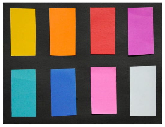
Figure 1.
Scanning scene of nine-color card papers, which are black, yellow, orange, red, purple, cyan, blue, pink, and white.
The second experiment was composed of seven different colored targets: black card paper, aloe leaves, white ceramic pot, red surface of a Rubik’s Cube, brown box, and green and orange parts of a ceramic doll. Among them, the white ceramic pot and the ceramic doll are the same material, but the colors are different. The targets, apart from the black card paper, were placed on a small horizontal platform at nearly the same distance from the laser source as the first experiment. A total of 2800 scanned points was measured. The scanning scene as shown in Figure 2.

Figure 2.
Scanning the scene of seven different colored targets.
3. Methods
3.1. Data Preprocessing
The availability of calibrated laser-based reflective intensity would be significant with respect to further spectral application [43]. The backscattered spectral intensities received by detectors are affected by laser incidence angle, distance, systematic noise, and surrounding atmospheric environment [44,45,46]. In this research, we considered only the laser incidence angle and distance factor, because the data was obtained in a clean dark laboratory where the atmospheric effect was minor. The accuracy of backscatter intensity was improved by using the distance and angle calibration model based on laser radar equation [47,48].
3.2. True-Color Composition
The color property depends on not only the illumination source, but also the visual characteristics of the human eyes. The reflective intensity of different bands in the visible light regions acquired by HSL creates a necessary condition for compositing true-color. The spectral intensities of different bands are different for perception of the human eyes, thus the spectral tristimulus values were established based on this visual characteristics [49]. The tristimulus values indicate the amount of radiant energy of the different bands in visible light regions, which will enter the human eyes. It takes two steps to convert spectral intensities into true-color. First, the chromaticity values are calculated based on the relationship between the spectral tristimulus values and the spectral intensities of the different bands by numerical integration method. The numerical integration was in the 431–751 nm spectral range. Second, the true-color values were obtained by converting the chromaticity values. Two processes performed in the CIE 1931 color space using a small visual angle 2°.
The color attributes were described by three component of hue, brightness, and saturation [50]. The hue refers to the style of color, which depends on the wavelength of light. The brightness indicates the lightness degree of color to the human eyes, while the saturation directs the purity of color. The calculated chromaticity values only denote the hue and saturation of the composition color, while the brightness cannot be obtained. To determine a certain color, in addition to determining the hue and saturation information, the brightness characteristic needs to be given. To intuitively represent color brightness, the Commission International de l’Eclairage ruled that the spectral tristimulus value was equivalent to the photopic luminous efficacy function [51]. Thus, an adjustment factor K introduced.
where X, Y, and Z are the chromaticity values. is the backscatter intensity of spectral bands. is the incident intensity of corresponding spectral bands. , , and are the tristimulus values of corresponding spectral bands in the CIE 1931 XYZ color space.
The using of sRGB is to define a rendered color space for data interchange in multimedia [52]. The true-color was obtained by converting chromaticity values into the sRGB color space. As the supercontinuum laser source simulated sunlight, the conversion matrix was determined based on standard illuminants of D65 [53].
In terms of the principle of three primary colors, true-color composition requires at least three spectral bands. Besides, the true-color composition is closely associated to the three primary color components of RGB, which were calculated using spectral intensities in the selected bands. Color distortions will occur if the color components are inaccurate. Therefore, the number and central wavelength of selected bands have an influence on the three primary color components. To verify the above statement, we selected different numbers and central wavelength of spectral bands by arithmetic progression from the 32 bands (Table 1) to composite true-color. The selected result consists of six schemes using 32, 16, 8, 5, and 3 spectral bands, especially in the fifth and sixth schemes, with the same number of bands, but different central wavelengths of the three bands.

Table 1.
Selection results of different number spectral bands.
The composition effect of true-color could be assessed via qualitative and quantitative analyses. Color vision is based on the physiological basis of visual perception, which can be seen as a powerful tool for evaluating the degree of color similarity. In quantitative analysis, the color similarity between the natural color of passive image (Figure 1) and the true-color composited by spectral intensities was assessed using linear discriminant analysis. We determined the pixel position in the passive image of each point in the point cloud by direct linear transformation [54]. Referring to a diffuse whiteboard (SpectraLon), which reaches approximately 100% reflectance, the three RGB channels reflectance of passive pixels and true-color point cloud were calculated. The three RGB channels reflectance of the true-color composited using spectral intensities was defined as the X-axis, while the three RGB channels reflectance of passive pixels was defined as the Y-axis. R-squared (R2) and root mean squared error (RMSE) were used as the assessment criteria for linear discriminant analysis. R2 indicates similar degree of color, while RMSE shows the deviation between truth-values and inversion values.
3.3. Wavelength Selection
Lacking partial spectral intensities in visible light regions, the color composition of three primary color components will be inaccurate, further leading to true-color distortions. The color distortions will also occur on our HSL system, yet it can be improved through wavelength selection method determining an optimal spectral band combination, which contains the largest amount of information and smallest correlation among all combinations. Two wavelength selection methods of PCA and SCM are selected based on this characteristic of the optimal combination [33,35]. The former highlights the amount of information of bands combination, while the latter centers the correlation between bands. Besides, in view of the cost of configured detection channels of HSL, three spectral bands were selected eventually from 32 spectral bands for compositing true-color.
In the PCA algorithm, principal component transformation are performed to calculate the contribution of each band to principal components, which is as an indicator for selecting optimal spectral bands. The spectral data, X = (x1, x2, …, xn), have the sample number m and dimension n.
where Y is the result of the principal component transformation, X is the matrix generated by subtracting the mean of each column from each column of spectral data X, and P is the matrix of principle component transformation. Transformation matrix P reflects the contribution between the ith wavelength (Xi) and the jth principal component (Yj). We can select an optimal band combination from 32 spectral bands based on this relation.
The correlation coefficient of spectral bands can be calculated by SCM [55]. The smaller is the correlation among the band combinations, the better is the independence and the lower is the redundancy. The optimal spectral bands can be determined by summing and ranking the correlations among the selected bands.
where T is the correlation between bands. is the correction coefficient between xth and yth bands. and are the autocorrelation coefficients of xth and yth spectral bands.
3.4. Target Classification
As one of the inherent attributes of targets, the true-color can be treated as a new classification feature. The classification potential of true-color was evaluated with seven different colored targets experiment. In total, 2800 measurement points manually labels via MATLAB, and the different color represented different targets. The manually labeled result as shown in Figure 3. We represented black card paper, aloe leaves, white ceramic pot, red surface of a Rubik’s Cube, brown box, and green and orange parts of a ceramic doll, with cyan, green, red, blue, orange, yellow, and mauve, respectively. The C-support Vector Classification based on libsvm and polynomial kernel function were employed [41]. In SVM training, the kernels, kernel parameters, and feature selection play key roles for SVM classification accuracy [56]. Bearing in mind that the optimal parameter determination is significant for a classification model with high stability and accuracy, we used a 10-fold cross-validation grid-search method to find the optimal parameter values of SVM. The parameter values of C and gamma were 1.4 and 1.1, respectively. Further, we also employed a Gaussian NB classifier to further verify true-color classification potential, which was a simple probabilistic classifier, and learned rapidly in various supervised classification problems [57]. The parameter of priors was 0. A three-fold cross validation was used to ensure the accuracy of target classification due to the limitation on the dataset [58]. We divided the data into three parts, using two-thirds of the data to train models, and the remaining data for testing. The overall classification accuracy can be calculated by predicted error sum of squares. Compared with other classification algorithms, SVM and NB were chosen in this study because it can get better classification results on small number of training sets [59,60]. The spectral reflectance of selected optimal bands and RGB values composited by spectral intensities of same spectral bands were used as the input parameters of SVM and NB classifier.
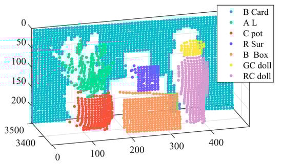
Figure 3.
Manually labeled hyperspectral LiDAR point cloud in the seven objects: black card paper, aloe leaves, white ceramic pot, red surface of a Rubik’s Cube, brown box, and green and orange parts of a ceramic doll, which are shown in cyan, green, red, blue, orange, yellow, and mauve, respectively.
4. Results and Discussion
4.1. True-Color Composition
The composition results of the selected bands in Table 1 as shown in Figure 4. The 32 (Figure 4a), 16 (Figure 4b), 8 (Figure 4c), and 5 (Figure 4d) spectral bands, and three spectral bands of different serials (Figure 4e,f) were used to composite the true-color. With the number and central wavelength of spectral bands changed, there were larger differences in the composition color of six schemes. The composition colors were evaluated via qualitative and quantitative analyses.
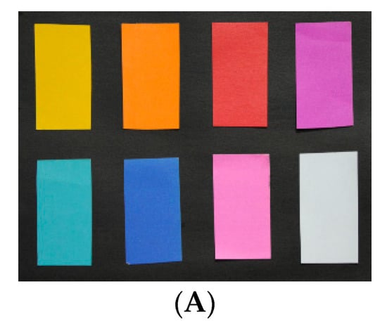
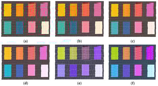
Figure 4.
The passive true-color image (A). The composition results of six schemes using 32 (a), 16 (b), 8 (c), 5 (d) spectral bands, and three spectral bands of different serials (e,f).
Through visual perception, the composition colors of the first four schemes (Figure 4a–d) were closer to a passive image (Figure 4A) acquired by a camera. Despite certain color distortions, the natural colors of the nine-color card papers can obtain with satisfactory visual effects in the first four schemes. In particular, compared to other schemes, the composited true-color of the fourth scheme (Figure 4d) was more vivid and the color similarity was higher. However, the two schemes of the fifth and sixth (Figure 4e,f) exhibited color distortions in different degrees and composited colors deviated to blue at the entire region. Especially in the fifth schemes, color distortions were more prominent and the composited color was nearly completely inconsistent with the natural color of nine-card papers. There were some color distortions in the sixth scheme, but the composited color still could show natural color. It was very significant to use appropriate number and central wavelength of spectral bands for compositing true-color based on above results.
The color similarity between the natural color of the passive image and the true-color composited by spectral intensities was assessed using linear discriminant analysis as Figure 5. Linear discriminant analysis of color similarity evaluated actual similarity degree of the three primary color components of R, G, and B between the composited true-color and natural color. Consistent with the results of the qualitative analysis, the first four schemes (Figure 5a–d) showed better results than the other two schemes (Figure 5e,f). Almost every R2 was more than 0.85, and RMSE was less than 1.866 in the first four schemes. The larger R2 and the smaller RMSE indicated the better composition result and the higher color similarity. In particular, the fourth scheme of five spectral bands had the best composition effect among the six schemes, whether in R2 or RMSE. The R2 of the three channels of R, G and B were 0.976, 0.9507, and 0.95, respectively, and all RMSEs were less than 1.264 in the fourth scheme. It needs to be noted that the R2 of the B channel gradually increased from 0.8422 to 0.95 with the decrease of the number of composited bands in the first four schemes when the R2 of R and G channels was nearly unchanged. The reason for this phenomenon was that the partial spectral intensities lacked in the process of compositing true-color, which ultimately led to inaccurate color components of RGB, further causing color distortions. In addition, since the central wavelengths of selected spectral bands were inaccurate, the poor results appeared in the two schemes of the fifth and sixth. The R2 of the G channel was less than 0.8, and some RMSEs were more than 1.9 in the fifth and sixth schemes. When all R2 of the three channels of RGB were higher and the RMSEs were lower in linear discriminant analysis, the composited results could be obtained with satisfactory visual effects and higher color similarity. This phenomenon can be reflected in the fourth and sixth schemes.
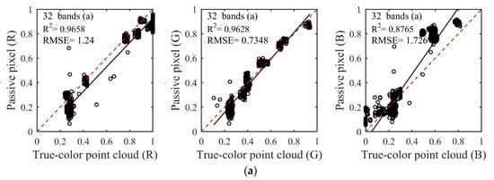
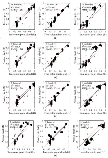
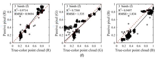
Figure 5.
The color similarity between the natural color of the passive image and the true-color composited by spectral intensities was assessed using linear discriminant analysis. (a–f) were linear discriminant analysis results with different schemes in Table 1. X-axis: three channels RGB reflectance of true-color point cloud. Y-axis: three channels RGB reflectance of the passive pixel. With the number of composition bands decreased, the composition results were better. Among them, the fourth scheme (d) had the best composition effect, and R2 were more than 0.9461 and RMSEs were less than 1.264.
To summarize, in the case of lacking partial spectral intensities in visible light bands, we must consider not only the number of composited bands, but also the central wavelength of spectral bands to achieve better true-color composition. Thus, selecting the optimal spectral bands from existing spectral bands for compositing true-color was significant.
4.2. Wavelength Selection
The three optimal spectral bands were selected by PCA and SCM for better compositing true-color, based on 32-dimensional spectral data of HSL. After PCA, the sum of the contributions of the first three principal components was more than 94%. By comparing the contributions of each band to the three principal components, the three spectral bands possessing largest amount of information were determined. The bands with the largest contribution to the three principal components as shown in Table 2.
Table 2.
PCA for selecting the optimal spectral bands.
The correlation between bands could be calculated by SCM. Allowing for the 32-dimensional spectrum, 4960 spectral band combinations were determined via the permutation and combination of . Ten-band combinations with the smallest correlation listed in Table 3, and the results are sorted in descending order.
Table 3.
The smallest correlations of spectral band combinations.
The spectral bands of 466, 536, and 626 nm had the smallest correlation among all the permutations and combinations. This optimal result was different from the result with 466, 546 and 626 nm determined by PCA. However, the difference between the two optimal combinations in the aspect of correlation was extremely small (0.0026). Given the correlation between 536 and 546 nm spectral being 99.36%, they can nearly replace each other. Therefore, jointly considering the two wavelength selection results, three spectral bands, namely, 466, 546, and 626 nm, were used as the optimal band combination for compositing true-color based on HSL system.
The composition effect and the result of linear discriminant analysis using the three spectral bands of 466, 546 and 626 nm as Figure 6. From the visual perception, the composited true-color can vividly show the natural color of the nine-color card papers, but the composited color was light yellow for the white card papers. The results of the linear discriminant analysis (Figure 6c) indicated that the R2 of three channels was more than 0.9191, while the RMSEs were less than 1.453. However, the composition effect was not perfect. Compared to the fourth scheme, the R2 of G and B channels was less than 0.9461, and the RMSE of each channel was high when three optimal spectral bands were used to composite true-color. The RMSE of three channels were 1.453, 0.931 and 1.367, which were higher than RMSEs of the fourth scheme. In addition to the reason already explained in Section 4.1, there is a second reason. The fourth scheme owned the larger abundant spectral information, resulting in a more accurate retrieval of RGB. This inaccuracy of three primary color components could be improved by using wavelength selections to determine the optimal spectral bands.
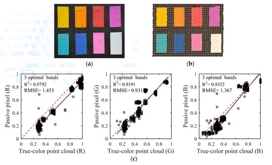
Figure 6.
The passive true-color image (a). The true-color point cloud (b) composited by 466, 546 and 626 nm. The linear discriminant analysis result (c) of three optimal bands between the composited true-color and natural color of the passive image.
4.3. RGB-Based Target Classification
The study area was classified into seven targets: black card paper, aloe leaves, white ceramic pot, red surface of a Rubik’s Cube, brown box, and green and orange parts of a ceramic doll. A total of 2800 scanned points was used, and three spectral reflectance (466, 546, and 626 nm) and RGB values composited by spectral intensities of the same three spectral were used as the input parameters of SVM and NB classifier. The confusion matrix and the overall accuracy for two classifiers were provided in Table 4 and Table 5. The classification result using the SVM classifier as shown in Figure 7.
Table 4.
The confusion matrix for SVM.
Table 5.
The confusion matrix for NB.
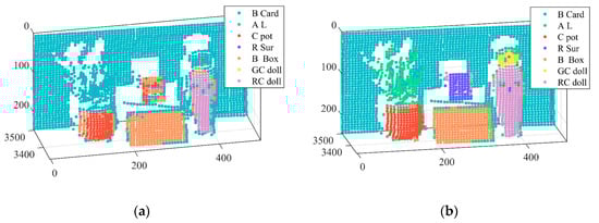
Figure 7.
Two classification results based on the three spectral reflectance of 466, 546, and 626 nm (a) and RGB values composited by spectral intensities of the same three spectral bands (b) using the SVM classifier. Different colors represent the different results of targets. The presentative color was the same as the training samples shown in Figure 3.
There were two classification results based on the three spectral reflectance of 466, 546, and 626 nm and RGB values composited by spectral intensities of the same three spectral bands using the SVM in Figure 7. These are clearly notable in Figure 7a, where nearly all points marked as green and yellow and a quarter of points marked as blue were misclassified as the black card papers. A quarter of points marked as red and half of points marked as pink were misclassified as the black card papers. The main reason was that the spectral features of these misclassified objects were similar in the color space where was constructed by the three spectral bands. Through the conversion of spectral intensities to true-color, the overall classification accuracy was increased by 14.6%. The user’s and producer’s accuracies of the seven targets were greatly improved, especially the producer’s accuracies of the aloe leaves, the red surface of a Rubik’s Cube, and the green parts of a ceramic doll, which increased from 0% to 75.56%, 87.23%, and 56%, respectively. The main reason for the limitation of improvement in the classification accuracy of the green ceramic doll was there were only 50 data, and there were many edge points.
The NB classifier produced diverse classification accuracies for the seven different colored objects in Table 5. The overall accuracies for two cases were 82.07% and 90.32%, based on a NB classifier. The classification accuracy was increased by 8.25% through the conversion between spectral intensities and true-color. As previously mentioned, the misclassified points with aloe leaves, white ceramic pot, red surface of a Rubik’s Cube, and green and orange parts of a ceramic doll were the main sources of classification errors using the three spectral bands. Especially, the producer’s accuracies of the red surface of a Rubik’s Cube, and the green and orange parts of a ceramic doll were increased from 0, 0.38, and 0.5136 to 0.8298, 0.72 and 0.8405, respectively.
The overall classification accuracy will be improved by converting spectral intensities into true-color information based on the above results. The classification result can be increased to 99.89% combining spatial information of targets. Moreover, many edge points were observed (Figure 7b), and they could affect the classification accuracy due to the changes in spectral intensities. A primary reason for these misclassified points was that the footprint of the laser beam might simultaneously illuminate two or more targets. The received reflected energy was composed of echo energy of different targets. The misclassified edge points can be eliminated by using the two-step classification method proposed by Chen et al. [24].
4.4. Inadequacies of the Proposed Method
One inadequacy of this true-color 3D imaging method is that determining three optimal spectral bands to composite true-color will cause spectral resource waste of HSL system. This spectral resource waste will increase color distortions to some extent. The retrieval accuracy of true-color will be increased if the spectral information in the blue-violet light regions can be obtained by spectral simulation.
Atmospheric effects can affect the backscatter intensities of the emitted laser [45]. Especially for airborne LiDAR, atmospheric effects are inevitable and difficult to account for [46]. This wavelength selection method does not consider the influence of atmospheric effects, which may influence spectral intensities of the selected spectral bands, further affecting true-color 3D imaging. Furthermore, more bands could be selected to realize target imaging without considering system cost.
The optimal spectral band combination is not fixed. It will vary with the spectral coverage of the HSL and the acquired spectrum must include the red, green and blue light regions. True-color composition using any three spectral bands has not been achieved.
5. Conclusions
The spatial and spectral information of targets obtains in one shot by HSL measurements, which is helpful for target imaging. In this study, the 32-dimensional HSL covering 431–751 nm spectral range was used and two color experiments were conducted. The experiment of nine-color card papers demonstrated the feasibility of a novel true-color three-dimensional (3D) imaging method based on HSL. In the case of low signal to noise in the blue-violet light regions, this study presented a combination of three spectral bands (466, 546, and 626 nm) for HSL system to invert true-color. The inversion results demonstrated that composited true-color can vividly show the natural color of nine-color card papers, and the color similarity between the natural color of the passive image and the true-color composited by spectral intensities was higher than 0.9191. The RGB feature can be used for target classification and the overall classification accuracy of seven different colored objects can reach up to 91.71% and 90.32% based on SVM and NB classifiers, respectively. Thus, target discrimination will be improved by converting spectral intensities into true-color. This study can serve as a guide in the design of new cost-effective and efficient true-color LiDAR systems, and could lay a foundation for the prevalence of the true-color LiDAR system for operational purposes.
Author Contributions
All authors made significant contributions to the work. W.G. and B.C. conceived and designed the experiments. S.S., K.G. and X.Z. performed the experiments. J.S., B.C., J.Y. and L.D. provided advice for the preparation and revision of the paper. B.C. wrote the paper.
Funding
This research received no external funding.
Acknowledgments
This work was supported by National Key R&D Program of China (Grant No. 2018YFB0504500), National Natural Science Foundation of China (Grant Nos. 41601360, 41571370, and 41801268), and Wuhan Morning Light Plan of Youth Science and Technology (2017050304010308).
Conflicts of Interest
The authors declare no conflict of interest.
References
- Tebaldini, S.; Rocca, F. Multibaseline polarimetric SAR tomography of a boreal forest at P-and L-bands. IEEE Trans. Geosci. Remote Sens. 2012, 50, 232–246. [Google Scholar] [CrossRef]
- Vaughan, R.G.; Hook, S.J.; Calvin, W.M.; Taranik, J.V. Surface mineral mapping at Steamboat Springs, Nevada, USA, with multi-wavelength thermal infrared images. Remote Sens. Environ. 2005, 99, 140–158. [Google Scholar] [CrossRef]
- Dale, L.M.; Thewis, A.; Boudry, C.; Rotar, I.; Dardenne, P.; Baeten, V.; Pierna, J.A.F. Hyperspectral imaging applications in agriculture and agro-food product quality and safety control: A review. Appl. Spectrosc. Rev. 2013, 48, 142–159. [Google Scholar] [CrossRef]
- Omasa, K.; Hosoi, F.; Konishi, A. 3D lidar imaging for detecting and understanding plant responses and canopy structure. J. Exp. Bot. 2006, 58, 881–898. [Google Scholar] [CrossRef] [PubMed]
- Garini, Y.; Young, I.T.; McNamara, G. Spectral imaging: Principles and applications. Cytom. Part A J. Int. Soc. Anal. Cytol. 2006, 69, 735–747. [Google Scholar] [CrossRef] [PubMed]
- Pan, Z.; Mao, F.; Wang, W.; Logan, T.; Hong, J. Examining Intrinsic Aerosol-Cloud Interactions in South Asia Through Multiple Satellite Observations. J. Geophys. Res. Atmos. 2018, 123, 11210–11224. [Google Scholar] [CrossRef]
- Botha, E.J.; Leblon, B.; Zebarth, B.; Watmough, J. Non-destructive estimation of potato leaf chlorophyll from canopy hyperspectral reflectance using the inverted PROSAIL model. Int. J. Appl. Earth Obs. Geoinf. 2007, 9, 360–374. [Google Scholar] [CrossRef]
- Li, Z.; Wu, E.; Pang, C.; Du, B.; Tao, Y.; Peng, H.; Zeng, H.; Wu, G. Multi-beam single-photon-counting three-dimensional imaging lidar. Opt. Express 2017, 25, 10189–10195. [Google Scholar] [CrossRef]
- Weibring, P.; Johansson, T.; Edner, H.; Svanberg, S.; Sundner, B.; Raimondi, V.; Cecchi, G.; Pantani, L. Fluorescence lidar imaging of historical monuments. Appl. Opt. 2001, 40, 6111–6120. [Google Scholar] [CrossRef]
- Lu, G.; Fei, B. Medical hyperspectral imaging: A review. J. Biomed. Opt. 2014, 19, 010901. [Google Scholar] [CrossRef]
- Thorp, K.; Tian, L. A review on remote sensing of weeds in agriculture. Precis. Agric. 2004, 5, 477–508. [Google Scholar] [CrossRef]
- Vaughan, R.G.; Calvin, W.M.; Taranik, J.V. SEBASS hyperspectral thermal infrared data: Surface emissivity measurement and mineral mapping. Remote Sens. Environ. 2003, 85, 48–63. [Google Scholar] [CrossRef]
- Lim, K.; Treitz, P.; Wulder, M.; St-Onge, B.; Flood, M. LiDAR remote sensing of forest structure. Prog. Phys. Geogr. 2003, 27, 88–106. [Google Scholar] [CrossRef]
- Nevalainen, O.; Hakala, T.; Suomalainen, J.; Kaasalainen, S. Nitrogen concentration estimation with hyperspectral LiDAR. ISPRS Ann. Photogramm. Remote Sens. Spat. Inf. Sci. 2013, II-5/W2, 205–210. [Google Scholar] [CrossRef]
- Gong, W.; Sun, J.; Shi, S.; Yang, J.; Du, L.; Zhu, B.; Song, S. Investigating the Potential of Using the Spatial and Spectral Information of Multispectral LiDAR for Object Classification. Sensors 2015, 15, 21989–22002. [Google Scholar] [CrossRef] [PubMed]
- Erdody, T.L.; Moskal, L.M. Fusion of LiDAR and imagery for estimating forest canopy fuels. Remote Sens. Environ. 2010, 114, 725–737. [Google Scholar] [CrossRef]
- Alonzo, M.; Bookhagen, B.; Roberts, D.A. Urban tree species mapping using hyperspectral and lidar data fusion. Remote Sens. Environ. 2014, 148, 70–83. [Google Scholar] [CrossRef]
- Du, L.; Gong, W.; Shi, S.; Yang, J.; Sun, J.; Zhu, B.; Song, S. Estimation of rice leaf nitrogen contents based on hyperspectral LIDAR. Int. J. Appl. Earth Obs. Geoinf. 2016, 44, 136–143. [Google Scholar] [CrossRef]
- Wei, G.; Shalei, S.; Bo, Z.; Shuo, S.; Faquan, L.; Xuewu, C. Multi-wavelength canopy LiDAR for remote sensing of vegetation: Design and system performance. ISPRS J. Photogramm. Remote Sens. 2012, 69, 1–9. [Google Scholar] [CrossRef]
- Suomalainen, J.; Hakala, T.; Kaartinen, H.; Räikkönen, E.; Kaasalainen, S. Demonstration of a virtual active hyperspectral LiDAR in automated point cloud classification. ISPRS J. Photogramm. Remote Sens. 2011, 66, 637–641. [Google Scholar] [CrossRef]
- Niu, Z.; Xu, Z.; Sun, G.; Huang, W.; Wang, L.; Feng, M.; Li, W.; He, W.; Gao, S. Design of a new multispectral waveform LiDAR instrument to monitor vegetation. IEEE Geosci. Remote Sens. Lett. 2015, 12, 1506–1510. [Google Scholar]
- Fernandez-Diaz, J.; Carter, W.; Glennie, C.; Shrestha, R.; Pan, Z.; Ekhtari, N.; Singhania, A.; Hauser, D.; Sartori, M. Capability assessment and performance metrics for the Titan multispectral mapping LiDAR. Remote Sens. 2016, 8, 936. [Google Scholar] [CrossRef]
- Sun, J.; Shi, S.; Yang, J.; Gong, W.; Qiu, F.; Wang, L.; Du, L.; Chen, B. Wavelength selection of the multispectral lidar system for estimating leaf chlorophyll and water contents through the PROSPECT model. Agric. For. Meteorol. 2019, 266, 43–52. [Google Scholar] [CrossRef]
- Chen, B.; Shi, S.; Gong, W.; Zhang, Q.; Yang, J.; Du, L.; Sun, J.; Zhang, Z.; Song, S. Multispectral LiDAR point cloud classification: A two-step approach. Remote Sens. 2017, 9, 373. [Google Scholar] [CrossRef]
- Yu, X.; Hyyppä, J.; Litkey, P.; Kaartinen, H.; Vastaranta, M.; Holopainen, M. Single-Sensor Solution to Tree Species Classification Using Multispectral Airborne Laser Scanning. Remote Sens. 2017, 9, 108. [Google Scholar] [CrossRef]
- Miller, C.I.; Thomas, J.J.; Kim, A.M.; Metcalf, J.P.; Olsen, R.C. Application of image classification techniques to multispectral lidar point cloud data. In Proceedings of the Laser Radar Technology and Applications XXI, Baltimore, MA, USA, 13 May 2016; p. 98320X. [Google Scholar]
- Puttonen, E.; Hakala, T.; Nevalainen, O.; Kaasalainen, S.; Krooks, A.; Karjalainen, M.; Anttila, K. Artificial target detection with a hyperspectral LiDAR over 26-h measurement. Opt. Eng. 2015, 54, 013105. [Google Scholar] [CrossRef]
- Wright, W.D. A re-determination of the trichromatic coefficients of the spectral colors. Trans. Opt. Soc. 1929, 30, 141. [Google Scholar] [CrossRef]
- Guild, J. The Colorimetric Properties of the Spectrum. Philos. Trans. R. Soc. Lond. 1932, 230, 149–187. [Google Scholar] [CrossRef]
- Shaw, M.; Fairchild, M. Evaluating the 1931 CIE color-matching functions. Color Res. Appl. 2002, 27, 316–329. [Google Scholar] [CrossRef]
- Schanda, J. Colorimetry: Understanding the CIE System; John Wiley & Sons, Ltd.: Hoboken, NJ, USA, 2007; ISBN 978-0-470-04904-4. [Google Scholar]
- Chen, H.; Liang, T.; Yao, J. The Processing Algorithms and EML Modeling of True Color Synthesis for SPOT5 Image. Appl. Mech. Mater. 2013, 373–375, 564–568. [Google Scholar] [CrossRef]
- Song, S.; Gong, W.; Zhu, B.; Huang, X. Wavelength selection and spectral discrimination for paddy rice, with laboratory measurements of hyperspectral leaf reflectance. ISPRS J. Photogramm. Remote Sens. 2011, 66, 672–682. [Google Scholar] [CrossRef]
- Van der Meer, F. The effectiveness of spectral similarity measures for the analysis of hyperspectral imagery. Int. J. Appl. Earth Obs. Geoinf. 2006, 8, 3–17. [Google Scholar] [CrossRef]
- Puttonen, E.; Suomalainen, J.; Hakala, T.; Räikkönen, E.; Kaartinen, H.; Kaasalainen, S.; Litkey, P. Tree species classification from fused active hyperspectral reflectance and LIDAR measurements. For. Ecol. Manag. 2010, 260, 1843–1852. [Google Scholar] [CrossRef]
- Popescu, S.C. Estimating biomass of individual pine trees using airborne lidar. Biomass Bioenergy 2007, 31, 646–655. [Google Scholar] [CrossRef]
- Foody, G.M.; Mathur, A. Toward intelligent training of supervised image classifications: Directing training data acquisition for SVM classification. Remote Sens. Environ. 2004, 93, 107–117. [Google Scholar] [CrossRef]
- Tarabalka, Y.; Fauvel, M.; Chanussot, J.; Benediktsson, J.A. SVM-and MRF-based method for accurate classification of hyperspectral images. IEEE Geosci. Remote Sens. Lett. 2010, 7, 736–740. [Google Scholar] [CrossRef]
- Vapnik, V. The Nature of Statistical Learning Theory; Springer Science & Business Media: New York, NY, USA, 2013. [Google Scholar]
- Chang, C.-C.; Lin, C.-J. LIBSVM: A library for support vector machines. ACM Trans. Intell. Syst. Technol. (TIST) 2011, 2. [Google Scholar] [CrossRef]
- Tien Bui, D.; Pradhan, B.; Lofman, O.; Revhaug, I. Landslide susceptibility assessment in vietnam using support vector machines, decision tree, and Naive Bayes Models. Math. Probl. Eng. 2012, 2012, 974638. [Google Scholar] [CrossRef]
- Kaasalainen, S.; Hyyppa, H.; Kukko, A.; Litkey, P.; Ahokas, E.; Hyyppa, J.; Lehner, H.; Jaakkola, A.; Suomalainen, J.; Akujarvi, A. Radiometric Calibration of LIDAR Intensity With Commercially Available Reference Targets. IEEE Trans. Geosci. Remote Sens. 2009, 47, 588–598. [Google Scholar] [CrossRef]
- Kaasalainen, S.; Jaakkola, A.; Kaasalainen, M.; Krooks, A.; Kukko, A. Analysis of Incidence Angle and Distance Effects on Terrestrial Laser Scanner Intensity: Search for Correction Methods. Remote Sens. 2011, 3, 2207–2221. [Google Scholar] [CrossRef]
- Höfle, B.; Pfeifer, N. Correction of laser scanning intensity data: Data and model-driven approaches. ISPRS J. Photogramm. Remote Sens. 2007, 62, 415–433. [Google Scholar] [CrossRef]
- Yan, W.Y.; Shaker, A. Radiometric correction and normalization of airborne LiDAR intensity data for improving land-cover classification. IEEE Trans. Geosci. Remote Sens. 2014, 52, 7658–7673. [Google Scholar]
- Shi, S.; Song, S.; Gong, W.; Du, L.; Zhu, B.; Huang, X. Improving backscatter intensity calibration for multispectral LiDAR. IEEE Geosci. Remote Sens. Lett. 2015, 12, 1421–1425. [Google Scholar] [CrossRef]
- Kaasalainen, S.; Krooks, A.; Kukko, A.; Kaartinen, H. Radiometric calibration of terrestrial laser scanners with external reference targets. Remote Sens. 2009, 1, 144–158. [Google Scholar] [CrossRef]
- Prasad, K.K.; Raheem, S.; Vijayalekshmi, P.; Sastri, C.K. Basic aspects and applications of tristimulus colorimetry. Talanta 1996, 43, 1187–1206. [Google Scholar]
- Shi, Y.; Ding, Y.; Zhang, R.; Li, J. Structure and hue similarity for color image quality assessment. In Proceedings of the 2009 International Conference on Electronic Computer Technology, Macau, China, 20–22 February 2009; pp. 329–333. [Google Scholar]
- Trussell, H.J.; Saber, E.; Vrhel, M. Color image processing: Basics and special issue overview. IEEE Signal Process. Mag. 2005, 22, 14–22. [Google Scholar] [CrossRef]
- Süsstrunk, S.; Buckley, R.; Swen, S. Standard RGB color spaces. In Proceedings of the Color and Imaging Conference, Scottsdale, AZ, USA, 16–19 November 1999; pp. 127–134. [Google Scholar]
- Asmare, M.H.; Asirvadam, V.S.; Iznita, L. Color space selection for color image enhancement applications. In Proceedings of the 2009 International Conference on Signal Acquisition and Processing, Kuala Lumpur, Malaysia, 3–5 April 2009; pp. 208–212. [Google Scholar]
- Zhang, X.; Zhang, A.; Meng, X. Automatic fusion of hyperspectral images and laser scans using feature points. J. Sens. 2015, 2015, 415361. [Google Scholar] [CrossRef]
- Meero, F.V.D.; Bakker, W. Cross correlogram spectral matching: Application to surface mineralogical mapping by using AVIRIS data from Cuprite, Nevada. Remote Sens. Environ. 1997, 61, 371–382. [Google Scholar] [CrossRef]
- Avci, E. Selecting of the optimal feature subset and kernel parameters in digital modulation classification by using hybrid genetic algorithm–support vector machines: HGASVM. Expert Syst. Appl. 2009, 36, 1391–1402. [Google Scholar] [CrossRef]
- Patil, T.R.; Sherekar, S. Performance analysis of Naive Bayes and J48 classification algorithm for data classification. Int. J. Comput. Sci. Appl. 2013, 6, 256–261. [Google Scholar]
- Wong, T.-T. Performance evaluation of classification algorithms by k-fold and leave-one-out cross validation. Pattern Recognit. 2015, 48, 2839–2846. [Google Scholar] [CrossRef]
- Mountrakis, G.; Im, J.; Ogole, C. Support vector machines in remote sensing: A review. ISPRS J. Photogramm. Remote Sens. 2011, 66, 247–259. [Google Scholar] [CrossRef]
- Ratanamahatana, C.A.; Gunopulos, D. Feature selection for the naive bayesian classifier using decision trees. Appl. Artif. Intell. 2003, 17, 475–487. [Google Scholar] [CrossRef]
- Challis, K.; Carey, C.; Kincey, M.; Howard, A.J. Airborne lidar intensity and geoarchaeological prospection in river valley floors. Archaeol. Prospect. 2011, 18, 1–13. [Google Scholar] [CrossRef]


© 2019 by the authors. Licensee MDPI, Basel, Switzerland. This article is an open access article distributed under the terms and conditions of the Creative Commons Attribution (CC BY) license (http://creativecommons.org/licenses/by/4.0/).