Abstract
In this study, absorption variation of chromophoric dissolved organic matter (CDOM) was investigated based on spectroscopic measurements of the water surface and bottom during a cruise survey on 2–12 May 2014 in the Pearl River Estuary (PRE). Multiple spectral signatures were utilized, including the absorption ratios E2/E3 (a(250)/a(365)) and E2/E4 (a(254)/a(436))) as well as the spectral slopes over multiple wavelength ranges. The horizontal variations of a(300), E2/E3, spectral slope (S) of Ultraviolet C (SUVC, 250–280 nm), Ultraviolet B (SUVB, 280–315 nm), and S275–295 (275–295 nm) were highly correlated, revealing that CDOM of terrigenous origin in the upper estuary contained chromophores of larger molecular size and weight, while the marine CDOM in the lower estuary comprised organic compounds of smaller molecular size and weight; the molecular size of surface CDOM was generally larger than that at the bottom. Results of Gaussian decomposition methods showed that CDOM in the middle estuary of terrigenous origin produced more Gaussian components per spectrum than those of marine origin in the lower estuary and the adjacent Hong Kong waters. The surface CDOM composition was more diverse than at the bottom, inferred by the finding that the average number of Gaussian components yielded per surface sample (5.44) was more than that of the bottom sample (4.8). A majority of components was centered below 350 nm, indicating that organic compounds with relatively simple structures are ubiquitous in the estuary. Components centered above 350 nm only showed high peaks at the head of the estuary, suggesting that terrigenous CDOM with chromophores in complex structures rapidly lose visible light absorptivity during its transport in the PRE. The relatively low and homogenous peak heights of the components in Hong Kong waters imply higher light stability and composition consistency of the marine CDOM compared with the terrigenous CDOM.
1. Introduction
Dissolved organic matter (DOM) is one of the earth’s largest exchangeable reservoirs of organic material and an important component of the marine biogeochemical system. It plays a significant role in the carbon cycle, climate change, and global habitability [1,2,3]. Measurements of DOM have been improved in recent years by using spectroscopic instruments which provide ease of use, fast response, and low cost [4]. The intensive sampling of DOM optical properties makes it possible to detect variations of DOM at a much higher temporal and spatial resolution [5]. However, the application of spectroscopic techniques in DOM studies is limited by inadequate understanding of the relationship between optical properties and biogeochemical processes of DOM, which still needs further investigation [6].
Chromophoric (or colored) dissolved organic matters (CDOM) is the light-absorbing fraction of DOM, which along with fluorescence DOM (FDOM) possesses major aspects of DOM optical characteristics. The ultraviolet–visible (UV–VIS) absorption spectrum of CDOM is regarded as a signature and tracer of DOM composition, source, and reactivity [4]. For example, absorption coefficients have been employed to quantify concentrations of CDOM, dissolved organic carbon (DOC), and certain organic materials such as lignin phenol and aromatic acids. The UV-band absorptions (i.e., 250–440 nm) are most often used to infer DOM concentration because most aromatic compounds have their absorption maxima in the UV range and are believed to contain more chemical information of CDOM composition than the visible wavelengths [5,7,8,9].
The absorption ratio, that is, the ratio of two CDOM absorption coefficients at different wavelengths, can act as a tracer for molecular weight (MW), humification degree, and the sources of DOM in natural environments ([4] and references therein). The absorption ratios proposed in previous studies include a(200–299)/a(300–399) (namely, E2/E3), a(200–299)/a(400–499) (namely, E2/E4), a(200–299)/a(600–699) (namely, E2/E6), and a(400–499)/a(600–699) (namely, E4/E6) [10,11,12,13]. The most effective tracer for CDOM molecular information is E2/E3 (a(250)/a(365)), which is typically negatively correlated with CDOM MW [11,14,15,16]. It is known that high molecular weight (HMW) CDOM has stronger absorption at longer wavelengths, while low molecular weight (LMW) CDOM is more photosensitive at shorter wavelengths; hence, a decrease of E2/E3 could indicate an increase in CDOM molecular size [17]. The ratio E2/E4 (a(254)/a(436)) was employed to identify the source of DOM (i.e., autochthonous or allochthonous) [12,18]. However, the E2/E6 and E4/E6 ratios are not recommended for natural CDOM investigation due to the poor quality of absorption measurements at longer wavelengths [17].
Spectral slope (S) describes the decrease in absorption rate with the increase in wavelength and can be obtained by fitting the absorption spectrum to an exponential model (Equation (1)) [19,20,21]:
where ag is the CDOM absorption coefficient, and λ0 is the reference wavelength. The wavelength range over which S is calculated is not fixed. Usually, S is calculated over a broad wavelength range (e.g., 250–700, 400–700, and 300–600 nm). Recent studies have shown that using S over narrow wavelength ranges (e.g., 275–295 nm, 350–400 nm, and the spectral slope curve) is more effective to infer the CDOM MW and source [17,22,23,24].
Different spectral ranges produce different spectral slopes because the CDOM absorption spectra do not exactly follow a continuous exponential decay with an increase in wavelength. This makes it difficult to compare S values across studies [6,25]. In addition to the spectral range, the choice of reference wavelength (λ0) in Equation (1) can also influence the value of S, as shown in Figure 1. The same wavelength range (250–700 nm) with different λ0 (350, 400, and 450 nm) yields different values of S (0.0102, 0.0093, and 0.0088 nm−1) and model residuals. A single exponential curve cannot adequately simulate the true shape of CDOM spectra; therefore, new modeling approaches have been proposed to reveal more characteristics such as shoulders, peaks, and deviations from the original absorption spectra. These improved models include hyperbolic fitting, double exponential fitting, piecewise regression, and Gaussian decomposition [6,25,26,27,28].
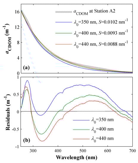
Figure 1.
In situ absorption spectrum measured in the Pearl River Estuary in May 2014 (thick gray line) and the exponential curves (colored lines) fitted to Equation (1). The fits were obtained over the same wavelength range (250–700 nm) but with a different reference wavelength (λ0), resulting in various spectral slope (S) values (see legend in (a)) and various residuals (see colored lines in (b)). The absorption spectrum sampled at the surface of Station A2 is used as an example (please refer to [29] for detailed information on Station A2).
In a previous investigation [29], the mixing behavior of CDOM in the Pearl River Estuary (PRE) was examined, revealing that CDOM with different sources (terrigenous or marine) and depths (surface or bottom) have distinct mixing characteristics (conservative or nonconservative). In this study, we focused on the horizontal and vertical variation of the absorption spectrum and its implication for CDOM chemical information. Absorption ratios and spectral slopes over diverse wavelength ranges were used as signatures to indicate CDOM molecular information. A Gaussian decomposition approach [6] was utilized to model the absorption spectra and identify absorptive components. A detailed analysis of the decomposed components was conducted to provide a better understanding of the CDOM composition variation in the PRE, which can benefit studies on DOM dynamics in the PRE and microscale biogeochemical processes in the estuarine and coastal area.
2. Materials and Methods
2.1. Absorption Spectra Collection
A cruise was carried out from 2 to 12 May 2014 in the Pearl River Estuary, adjacent to the northern South China Sea. A total of 148 water samples were collected from the water surface (with a sampling depth of 0–1 m) and the bottom (with a sampling depth 1 m above the bottom) (Figure 2), then filtered through 0.2 µm Millipore polycarbonate filters to obtain the CDOM filtrates. CDOM absorbance (A(λ)) was measured in a 10 cm curvette using a Shimadzu UV-2550 spectrophotometer (please refer to [29] for more detailed information about the in situ sampling). The absorption coefficients (a(λ)) over 250–700 nm at 1 nm resolution were calculated by
where L is the optical path length (here, 0.1 m). An extrapolation equation (Equation (3)) was used to correct the scattering by residual particles in filtered samples if a(700) was larger than 0 [20] (Figure 3):
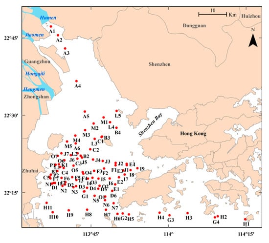
Figure 2.
Location of the sampling stations for the May 2014 cruise in the Pearl River Estuary.
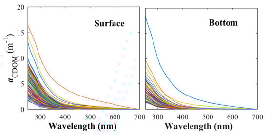
Figure 3.
Chromophoric dissolved organic matter (CDOM) absorption curves over the wavelength range of 250–700 nm, measured at the water surface and at the bottom in the Pearl River Estuary.
2.2. Spectral Slopes and Absorption Ratios
The UV range is where most CDOM components have their maximum absorptivity and where the CDOM absorption shifts substantially during its transport and photochemical alteration in the estuary [17]. Spectral slopes calculated in the UV range can provide more information on CDOM molecular and compositional changes in the estuarine mixing process. Thus, the spectral slopes were calculated separately in two observational bands: UV (250–400 nm) and VIS (400–700 nm). The UV band was further divided into UVC (250–280 nm), UVB (280–315 nm), and UVA (315–400 nm) to provide a better fit to the observed spectra. These independent spectral domains produced multiple values of S, which could reveal more information about the CDOM variation in the PRE. The widely used spectral slopes S275–295 (275–295 nm) and S350–400 (350–400 nm) and their ratio SR (S275–295/S350–400) were also calculated. The reference wavelengths (λ0) were selected as 265, 300, 360, 400, 285, and 375 nm for UVC (250–280 nm), UVB (280–315 nm), UVA (315–400 nm), VIS (400–700 nm), 275–295 nm, and 350–400 nm, respectively. A nonlinear least-squares curve fitting procedure was applied to Equation (1) to obtain the S values.
The absorption ratios E2/E3 (a(250)/a(365)) and E2/E4 (a(254)/a(436)) were used in this study to infer the CDOM molecular information in the PRE. The two ratios were expected to provide a general depiction of the horizontal and vertical variation of CDOM molecular size and weight in the estuary.
2.3. Gaussian Decomposition Approach
The Gaussian decomposition approach assumes that the deviations (e.g., shoulders and peaks) of absorption spectra from a standard exponential pattern are caused by the presence of certain compounds or structures in significant amounts [6]. Therefore, the absorption spectra can be separated into two parts. The first part is the theoretical exponential decay curve (defined as the baseline), and the second part represents the deviation from the theoretical curve (defined as the residuals). The Gaussian decomposition approach is used to model the residuals and decompose the residuals into individual Gaussian components. These Gaussian components are assumed to be connected with the absorption of certain individual chromophores [6]. The probability density function of a Gaussian curve with three parameters is given by
where ϕ (m−1) is the height of the curve peak (), μ (nm) is the wavelength of the peak, and σ (nm) is the standard deviation representing the width of the curve. The linear combination of the exponential baseline (Equation (1)) and several individual Gaussian components constitutes a new model to fit the CDOM absorption spectra, given by
where i = 1…n denotes a particular Gaussian component, and ε is the residual error.
The exponential baselines were obtained following the methodology in [6], using an iterative procedure in which the exponential model (Equation (1)) was fitted by a least-squares method to the spectrum after the wavelengths with all evident peaks or shoulders were identified and removed, and the remaining residuals were less than the absolute average residual [6]. The residual curves were calculated by removing the baselines from the original spectra. The values of the Gaussian parameters (ϕ, μ, σ) were determined by fitting the residual curves to Gaussian models with one to eight components and were constrained, following [6]. The optimal number of Gaussian components to fit a residual curve was identified by the Bayesian information criterion (BIC) to avoid overfitting. The BIC was calculated using the maximized model likelihood function, the observation number, and the parameter number. Among the eight Gaussian models, the one with the lowest BIC score was selected. Since some CDOM samples still have strong absorption in the visible band, the decomposition was performed over the full wavelength range (250–700 nm) to capture all spectral characteristics.
The exponential curve fitting, Gaussian decomposition, and BIC score calculation were implemented with MATLAB R2011a (www.mathworks.com). The MATLAB fitting toolbox (Curve Fitting Tool) was used to determine the Gaussian parameters. The aicbic function was used to calculate BIC scores. The statistical analysis of the decomposed Gaussian components was conducted by using SPSS Statistics 19 (Descriptive Statistics-Frequency/Description). The Kriging interpolation was used to map the distribution pattern in the PRE.
3. Results
3.1. Spectral Slopes and Absorption Ratios
The S value over the UVB band (SUVB; 280–315 nm) was the highest among all spectral components (range of 0.0127–0.0303 nm−1 with averages of 0.0184 nm−1 at the surface and 0.0208 nm−1 at the bottom), followed by S over the UVA band (SUVA; 315–400 nm) and S over the visible band (SVIS; 400–700 nm) (Table 1). The S over the UVC band (SUVC; 250–280 nm) had the smallest values, in a range of 0.0076–0.0183 nm−1 with averages of 0.0121 nm−1 at the surface and 0.0132 nm−1 at the bottom, showing a pronounced shoulder at 250–280 nm. The S275–295 and S350–400 were quantitatively close to SUVB and SUVA, respectively, due to the similar spectral range employed for S calculation (Table 1). The spectral slope ratio SR varied in the range of 0.72–2.93, with an average of 1.20 both at the surface and the bottom. The E2/E3 ratio in the PRE had a range of 3.11–13.27 with an average of 6.94 at the surface and 7.22 at the bottom. The E2/E4 ratio was more varied than E2/E3, ranging from 4.71 to 37.73 with an average of 19.26 at the surface and 18.96 at the bottom (Table 1). Significant correlations were found between E2/E3 and SUVB at both the surface and the bottom (Figure 4), with an r2 of 0.79 and 0.54, respectively. Better correlations existed between E2/E4 and SUVA (Figure 4), with an r2 of 0.89 at the surface and 0.83 at the bottom. These strong correlations illustrate the consistency of absorption ratios and spectral slopes in describing the spectral shapes of CDOM absorption if they are calculated in the similar spectral range.

Table 1.
The variation range, mean value, and standard deviation (SD) of the surface and bottom CDOM absorption coefficient at 300 nm (a(300)); spectral slopes SUVC (250–280 nm), SUVB (280–315 nm), SUVA (315–400 nm), SVIS (400–700 nm), S275–295 (275–295 nm), and S350–400 (350–400 nm); spectral slope ratio SR (S275–295/S350–400); absorption ratios E2/E3 (a(250)/a(365)) and E2/E4 (a(254)/a(436)); the peak height of the residual curve (Φ); the proportion of residuals from the original absorption at the peak position (%Residual); the number of Gaussian components decomposed per spectrum (N); and the peak height (φ), peak position (µ), and width (σ) of the Gaussian components in the Pearl River Estuary.
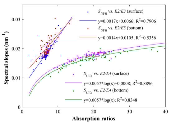
Figure 4.
Scatter plot of surface and bottom spectral slope as a function of absorption ratio over a similar wavelength range: SUVB (280–315 nm) versus E2/E3 (a(250)/a(365)), and SUVA (315–400 nm) versus E2/E4 (a(254)/a(436)).
The spatial variation of the absorption coefficient (a(300)); the absorption ratio of E2/E3 (a(250)/a(365)); and the spectral slopes of SUVC, SUVB, and S275–295 in the PRE revealed a consistent trend (Figure 5a,c,e,g,i). At the head of the estuary, where the water property is greatly influenced by upstream terrigenous inputs, CDOM observations showed larger values of a(300) and smaller values of E2/E3, SUVC, SUVB, and S275–295 at both the surface and the bottom. During the water transport from the upper estuary to the downstream region along the northwest–southeast path, a(300) decreased; E2/E3, SUVC, SUVB, and S275–295 increased; and the surface–bottom difference gradually expanded, with larger a(300) and smaller E2/E3, SUVC, SUVB, and S275–295 at the surface. The lowest level of a(300) and highest level of E2/E3, SUVC, SUVB, and S275–295 occurred in the southeastern estuary and the coastal regions of Hong Kong, dominated by higher saline coastal water. The surface E2/E3, SUVC, SUVB, and S275–295 were lower than the bottom in this area.
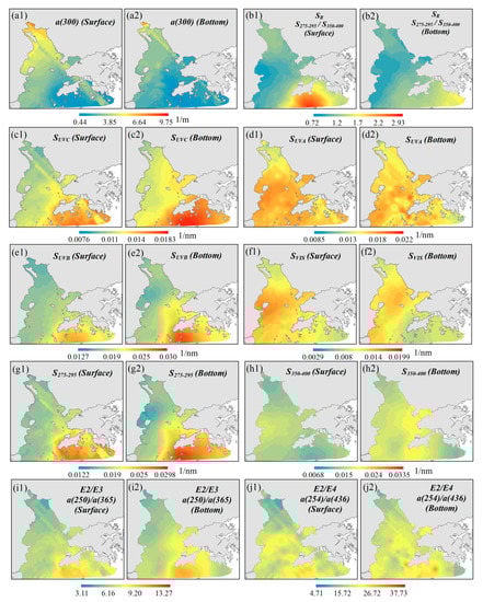
Figure 5.
Surface and bottom variation of: (a) CDOM absorption a(300); (b) the spectral slope ratio SR (S275–295/S350–400); (c–h) spectral slopes SUVC (250–280 nm), SUVB (280–315 nm), SUVA (315–400 nm), SVIS (400–700 nm), S275–295 (275–295 nm), and S350–400 (350–400 nm); and (i,j) absorption ratios E2/E3 (a(250)/a(365)) and E2/E4 (a(254)/a(436)) in the Pearl River Estuary. All figures were mapped by the Kriging interpolation method based on discrete sampling data.
Since E2/E3 and S275–295 are known to be negatively correlated with CDOM MW, the highly consistent distribution pattern of E2/E3, SUVC, SUVB, and S275–295 revealed that the CDOM of terrigenous origin in the upper estuary contains chromophores of larger molecular size and weight, while the marine CDOM in the lower estuary and the Hong Kong coastal waters comprises organic compounds of smaller molecular size and weight. The vertical variation of the spectral signatures indicated that the molecular size of surface CDOM is larger than that at the bottom, especially in the eastern and lower area of the estuary.
The distribution pattern of SR differed slightly from E2/E3, SUVC, SUVB, and S275–295. As determined by S275–295 and S350–400, the smallest SR occurred in the western estuary rather than at the head. The SR then increased gradually towards the north and south and was the largest in the southeastern estuary and near the Hong Kong waters (Figure 5b). The surface–bottom variation of SR was only prominent near Hong Kong. The variations of E2/E4, SUVA, SVIS, and S350–400 lacked any uniform pattern, either horizontally or vertically (Figure 5d,f,h,j).
3.2. Gaussian Decomposition
Figure 6a,b show the baselines and residuals separated from the observed CDOM absorption spectra. The baselines maintained the standard exponential pattern, whereas the residuals showed significant peaks in the wavelength range of 264–313 nm, with an average position near 280 nm. The peak height of the residuals varied between 0.12 and 6.13 m−1 and accounted for an average of 43.8% of the original absorption intensity at the peak position. The residuals possessed a large proportion of absorption (>40%) throughout the estuary, while lower percentage values (<20%) were observed in the waters near Hong Kong (Figure 7b).
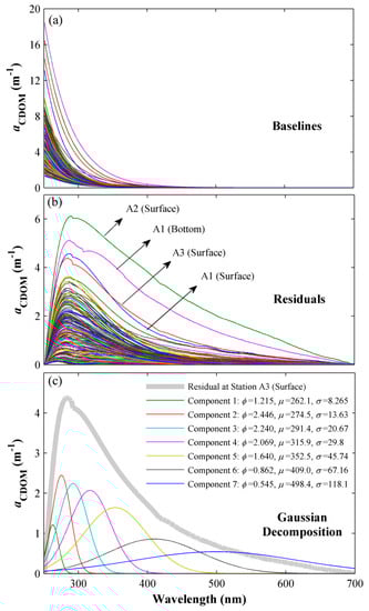
Figure 6.
The (a) baselines, (b) residuals, and (c) Gaussian components separated from CDOM absorption spectra collected in the Pearl River Estuary at the surface and bottom. The gray line in (c) is the residual curve of a surface sample (Station A3); the colored lines are the seven decomposed Gaussian components. The peak height (φ), peak position (μ), and curve width (σ) of the components are listed in the legend.
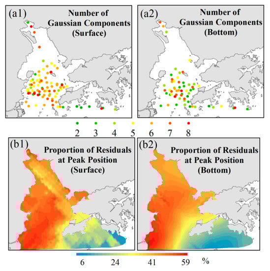
Figure 7.
Surface and bottom variation of (a) the number of Gaussian components decomposed per spectrum and (b) the proportion of residuals from the original absorption at the peak position. Figures in (b) were mapped by the Kriging interpolation method based on discrete sampling data.
Gaussian decomposition was performed on the 88 residual curves at the surface and 60 curves at the bottom, which yielded 479 and 288 Gaussian components at the surface and bottom, respectively. An example of the Gaussian components decomposed from a residual curve is shown in Figure 6c. The number of Gaussian components decomposed from a single spectrum was between 2 and 8, with the average number per spectrum of 5.44 at the surface and 4.8 at the bottom. Figure 7a shows the variation of the Gaussian component number per spectrum at both the surface and bottom. The samples in the middle area of the estuary produced more Gaussian components than those in the southeastern region and the Hong Kong water area, and the contrast is particularly significant at the bottom. Vertically, the surface spectra yielded more Gaussian components than the bottom spectra.
The frequency histograms of the peak height (ϕ), peak position (wavelength, μ), and the width (σ) of the Gaussian components at the surface and bottom are shown in Figure 8. The peak height of the components varied over a range of 0.015–2.934 m−1 at the surface and 0.007–2.612 m−1 at the bottom. The average values (0.6889 and 0.4614 m−1 for the surface and bottom, respectively) were much larger than those reported previously (0.0187 m−1) in [6]. The frequency decreased slowly towards larger peaks (Figure 8a). The peak position of all Gaussian components was in the range of 250–650 nm with a mean of 318 nm at the surface and 330.5 nm at the bottom. The bottom components tended to have peaks at longer wavelengths than the surface. The frequency distribution of the peak position (Figure 8b) identified eight groups at 262, 294, 319, 349, 402, 461, 498, and 546 nm at the surface. The bottom groups were at 272, 304, 333, 384, 405, 477, and 525 nm, slightly different from those at the surface. Nearly half of the total components had peaks below 300 nm, and the peak occurrence decreased sharply with the wavelength increase. Most Gaussian components had a width of less than 100 nm, with an average of 39.2 ± 38.9 nm at the surface and 43.6 ± 43.5 nm at the bottom (Figure 8c).
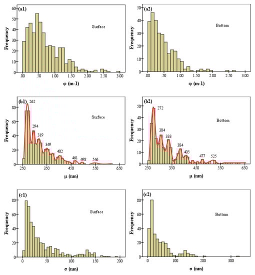
Figure 8.
The frequency histogram of (a) peak height (ϕ), (b) peak position (μ), and (c) curve width (σ) of the 479 Gaussian components at the surface (left column) and 288 components at the bottom (right column). Eight groups were identified from the surface components and labeled in (b1); seven groups were identified from the bottom components and labeled in (b2).
To further investigate the spatial variation of Gaussian components, five groups with relatively high frequency (centered near 260, 275, 300, 350, and 400 nm) were selected, and the peak heights of the components in each group are shown at their geographical locations in Figure 9. The size of the dots denotes the peak height of the Gaussian components; a larger size represents a higher peak. For all groups at the surface and bottom, the components located in the western estuary had larger peak heights than those in the eastern and southern area; the surface components had higher peaks than the bottom ones. The peak height of the components also varied among groups. For the average value, the group centered at 300 nm had the highest peak, followed in sequence by the group centered at 275, 350, 260, and 400 nm at both the surface and the bottom.
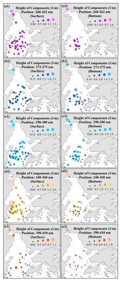
Figure 9.
Surface and bottom variations of peak height of Gaussian components in groups centered near wavelengths of (a) 260, (b) 275, (c) 300, (d) 350, and (e) 400 nm. The size of the dots denotes the peak height: the bigger the size, the higher the peak.
4. Discussion
4.1. Spectral Signatures
Previous efforts have demonstrated that the absorption ratios and spectral slopes are good indicators of CDOM molecular size and weight [5,30,31,32]. One possible mechanism leading to this connection is that the conjugation of electron donors on aromatic rings may affect the molar absorptivity of a chromophore and its spectral characteristic; the relatively simple aromatic compounds often have strong absorption at wavelengths below 300 nm. As the degree of conjugation and substitution increases, the wavelength of maximum absorption increases, and the spectra broaden [5]. On the other hand, the degree of conjugation determines the molecular size and weight of CDOM. The higher the degree of conjugation, the larger the molecular size and weight. Therefore, HMW CDOM tends to have higher absorption at longer wavelengths, leading to smaller values of absorption ratios and spectral slopes in certain wavelength ranges, and vice versa. One external force that can trigger CDOM molecular alteration is irradiation by sunlight, which can efficiently break the conjugation of the aromatic rings and convert the HMW chromophores to LMW [5], causing some spectral indicators such as E2/E3 and S275–295 to increase, while others such as S350–400 will decrease [17,33].
However, the spectral ranges involved in the identification of CDOM molecular properties are not globally uniform. For example, the values of S350–400, previously reported to decrease during photobleaching, did not show any obvious trends during our cruise in the PRE (see Figure 5h), making the recommended spectral slope ratio SR (S275–295/S350–400) (e.g., [17]) insufficient to uncover the whole picture of CDOM variation in the PRE. The situation was the same for E2/E4 (a(254)/a(436)), SUVA, and SVIS. S275–295 was shown to be a reliable indicator considering its consistent variation pattern with other signatures (E2/E3, SUVC, and SUVB) in the PRE. SUVB is particularly recommended for two reasons: (1) for its strong correlation with E2/E3 (a(250)/a(365)) (Figure 4) and (2) for its spectral range (280–315 nm), which simultaneously covers the wavelengths below and above 300 nm. This range seems more suitable to trace the CDOM absorptivity evolution during the electron-transition-induced alteration from HMW to LMW.
4.2. Gaussian Decomposition
Light absorption by a chromophore is determined by its intensity and nature [5]. According to the Beer–Lambert law, the molar absorptivity and concentration of the chromophore determine its absorption intensity. The electronic transitions involved influence the spectral shape. Therefore, the absorption spectrum of a chromophore can reflect its concentration and structure. However, the absorption curve currently obtained from a natural CDOM sample is an integration of overlapped spectra produced by multiple chromophores, resulting in obstructions in interpreting single chromophores from the synthetic spectrum. The Gaussian decomposition approach provides a way to identify individual absorption units and casts new light on studying CDOM composition variation in water masses [6]. This is particularly important for an estuary such as the PRE.
The Pearl River is China’s second largest river in terms of water discharge, exceeding 20,000 m3 s−1 in the flood season. Large amounts of river water flow out through four gates into the PRE, moving along the western estuary and southward to the mouth. Due to bottom topography and tidal effects, the seawater frequently intrudes into the estuary along the east shore. The downward-transported freshwater and the upward-moving seawater meet in the middle estuary, making the CDOM composition rather complicated in this area, which is illustrated by Figure 7a. The CDOM samples collected in the middle estuary tended to produce more Gaussian components per spectrum (varying between five and eight). In contrast, the samples obtained in the Hong Kong water yielded on average only two to three components per spectrum, indicating a less abundant CDOM composition. Vertically, the spectra of most samples resolved more components at the surface, suggesting a relatively simple CDOM composition at the bottom. The influence of source on CDOM composition was also indicated by the Gaussian decomposition results: the samples collected at the head of the estuary, which were dominated by terrigenous CDOM, resolved seven to eight Gaussian components per spectrum, far more than those in the Hong Kong water of marine origin.
With the assumption that the absorption of simpler organic compounds is mainly limited to shorter wavelengths (below 300 or 350 nm), while more complex structures have stronger absorptivity at longer wavelengths (above 350 nm) [5], the dynamics of the CDOM composition can be inferred by the variation of the Gaussian components centered at different wavelengths, shown in Figure 9. The larger number of components in the groups centered below 350 nm both at the surface and the bottom (Figure 9a,d) indicates that the organic compounds with simpler structures are ubiquitous in the estuary, possibly because most of them belong to refractory DOM [34], thus having a longer residence time in water. These components are also able to maintain a considerable level of absorptivity, inferred by their relatively large peak heights. Fewer components show peaks in the groups centered above 350 nm, with peak heights decreasing rapidly from north to south (Figure 9e), which implies that the terrigenous HMW CDOM tends to lose absorptivity quickly during water transport in the estuary, either due to biotic consumption or abiotic removal processes such as phototransformation, adsorption, and hydrothermal circulation [1,35]. Figure 9 also shows that the components in the Hong Kong water keep a relatively homogenous and low level of absorptivity for all the wavelength groups, indicating higher light stability and composition consistency of the marine CDOM.
The absorption peaks at certain wavelengths and the chromophores contributing to the peaks have been long established. For example, it was found that purine and pyrimidine rings contribute to an observed peak at 265 nm [36]. The peak was later discovered by [20] as a weak shoulder in seawater. This helps explain the slight shoulder observed in this study in the spectral range of 250–280 nm. The observed CDOM absorption at shorter wavelengths (<350 nm) is attributed to a mixture of a group of benzoic-acid-based derivatives and amino acids, while the longer wavelength absorption may be due to more complicated conjugated structures such as flavins, melanins, and tannins [5,37]. A recent study identified two distinct chromophores centered at 302 and 415 nm from the absorption spectrum of a humic substance in the dark ocean, which were proposed as the secondary absorption peak of nitrate and cytochrome c, respectively [27]. Our Gaussian decomposition results show a considerable number of components centered near 302 nm (17 at the surface and 13 at the bottom), while only a few components centered near 415 nm, which implies the high level of nitrate DOM and low concentration of cytochrome c in the PRE.
5. Conclusions
In this study, we analyzed the CDOM absorption spectra in the Pearl River Estuary in spring based on spectroscopic measurements at the water surface and bottom. Several spectral signatures, including the absorption ratios E2/E3 (a(250)/a(365)) and E2/E4 (a(254)/a(436))) as well as the spectral slopes over different wavelength ranges (SUVC (250–280 nm), SUVB (280–315 nm), SUVA (315–400 nm), SVIS (400–700 nm), S275–295 (275–295 nm), and S350–400 (350–400 nm)), were employed to investigate the horizontal and vertical variations of CDOM molecular information in the PRE. The horizontal variation of a(300), E2/E3, SUVC, SUVB, and S275–295 exhibited a highly consistent pattern, which illustrated that in the upper freshwater area of the estuary, HMW chromophores with a more complex structure were present, resulting in larger a(300) and smaller E2/E3, SUVC, SUVB, and S275–295. The lower estuary and the Hong Kong coastal waters contained more marine CDOM with LMW, leading to smaller a(300) and larger E2/E3, SUVC, SUVB, and S275–295. The vertical variation, shown by the surface–bottom difference of these indicators, was much larger in the middle and lower area of the estuary. SUVB is particularly recommended in CDOM investigations because of its strong correlation with E2/E3 and the molecularly meaningful spectral range of 280–315 nm.
A Gaussian decomposition approach was applied to the absorption spectra of CDOM to resolve individual absorptive components. The variation of the decomposition number revealed that the CDOM samples collected in the middle area of the estuary were more complicated in composition than those in the lower estuary and the Hong Kong waters, and the composition of CDOM at the bottom was much simpler than at the surface. This also implies that CDOM of terrigenous origin has a more abundant composition than those of marine origin. The spatial distributions of the decomposed components centered at different wavelength groups indicate that organic compounds with relatively simple structures are ubiquitous in the estuary, while terrigenous CDOM with high molecular weight tend to degrade quickly. The marine CDOM are suggested to be more optically stable and uniform in composition.
However, the indications of Gaussian decomposition methods are based on observations from the literature and have not yet been supported by direct chemical measurements and analysis of the relevant chemicals in the PRE. Therefore, further validation is still needed.
Author Contributions
All coauthors made significant contributions to this paper: conceptualization, X.L. and J.P.; methodology, X.L.; software, X.L.; validation, X.L., and J.P.; formal analysis, X.L.; investigation, J.P.; resources, A.T.D.; data curation, X.L.; writing—original draft preparation, X.L.; writing—review and editing, J.P. and A.T.D.; visualization, X.L.; supervision, J.P. and A.T.D.; project administration, J.P.; funding acquisition, J.P.
Funding
This research was supported by the National Natural Science Foundation of China (grant number 41376035), the General Research Fund of Hong Kong Research Grants Council (RGC) (grant numbers CUHK 14303818, 402912, and 403113), and the talent startup fund of Jiangxi Normal University.
Acknowledgments
The authors are grateful to the anonymous reviewers for their valuable suggestions and comments.
Conflicts of Interest
The authors declare no conflict of interest. The funders had no role in the design of the study; in the collection, analyses, or interpretation of data; in the writing of the manuscript; or in the decision to publish the results.
References
- Carlson, C.; Hansell, D. DOM sources, sinks, reactivity, and budgets. In Biogeochemistry of Marine Dissolved Organic Matter, 2nd ed.; Hansell, D., Carlson, C., Eds.; Academic Press: San Diego, CA, USA, 2015; pp. 65–125. [Google Scholar]
- Ducklow, H.W. Forword. In Biogeochemistry of Marine Dissolved Organic Matter; Hansell, D., Carlson, C., Eds.; Academic Press: San Diego, CA, USA, 2002; pp. xv–xix. [Google Scholar]
- Azam, F. Forword. In Biogeochemistry of Marine Dissolved Organic Matter, 2nd ed.; Hansell, D., Carlson, C., Eds.; Academic Press: San Diego, CA, USA, 2015; pp. xiii–xv. [Google Scholar]
- Li, P.; Hur, J. Utilization of UV-Vis spectroscopy and related data analyses for dissolved organic matter (DOM) studies: A review. Crit. Rev. Environ. Sci. Technol. 2017, 47, 131–154. [Google Scholar] [CrossRef]
- Stedmon, C.A.; Nelson, N.B. The optical properties of DOM in the ocean. In Biogeochemistry of Marine Dissolved Organic Matter, 2nd ed.; Hansell, D., Carlson, C., Eds.; Academic Press: San Diego, CA, USA, 2015; pp. 481–508. [Google Scholar]
- Massicotte, P.; Markager, S. Using a Gaussian decomposition approach to model absorption spectra of chromophoric dissolved organic matter. Mar. Chem. 2016, 180, 24–32. [Google Scholar] [CrossRef]
- Peacock, M.; Burden, A.; Cooper, M.; Dunn, C.; Evans, C.D.; Fenner, N.; Freeman, C.; Gough, R.; Hughes, D.; Hughes, S.; et al. Quantifying dissolved organic carbon concentrations in upland catchments using phenolic proxy measurements. J. Hydrol. 2013, 477, 251–260. [Google Scholar] [CrossRef]
- Osburn, C.L.; Boyd, T.J.; Montgomery, M.T.; Coffin, R.B.; Bianchi, T.S.; Paerl, H.W. Optical proxies for terrestrial dissolved organic matter in estuaries and coastal waters. Front. Mar. Sci. 2016, 2, 127. [Google Scholar] [CrossRef]
- Fichot, C.G.; Benner, R.; Kaiser, K.; Shen, Y.; Amon, R.M.W.; Ogawa, H.; Lu, C.J. Predicting dissolved lignin phenol concentrations in the coastal ocean from chromophoric dissolved organic matter (CDOM) absorption coefficients. Front. Mar. Sci. 2016, 3, 7. [Google Scholar] [CrossRef]
- Chen, Y.; Senesi, N.; Schnitzer, M. Information provided on humic substances by E4:E6 ratios. Soil Sci. Soc. Am. J. 1977, 41, 352–358. [Google Scholar] [CrossRef]
- Haan, D.H.; Boer, T.D. Applicability of light absorbance and fluorescence as measures of concentration and molecular size of dissolved organic carbon in humic Lake Tjeukemeer. Water Res. 1987, 21, 731–734. [Google Scholar] [CrossRef]
- Battin, T.J. Dissolved organic matter and its optical properties in a black water tributary of the upper Orinoco river, Venezuela. Org. Geochem. 1998, 28, 561–569. [Google Scholar] [CrossRef]
- Cieslewicz, J.; Gonet, S.S. Properties of humic acids as biomarkers of lake catchment management. Aquat. Sci. 2004, 66, 178–184. [Google Scholar] [CrossRef]
- Peuravuori, J.; Pihlaja, K. Molecular size distribution and spectroscopic properties of aquatic humic substances. Anal. Chim. Acta. 1997, 337, 133–149. [Google Scholar] [CrossRef]
- Erlandsson, M.; Futter, M.N.; Kothawala, D.N.; Kohler, S.J. Variability in spectral absorbance metrics across boreal lake waters. J. Environ. Monit. 2012, 14, 2643–2652. [Google Scholar] [CrossRef] [PubMed]
- Santos, L.; Pinto, A.; Filipe, O.; Cunha, A.; Santos, E.B.H.; Almeida, A. Insights on the optical properties of estuarine DOM? Hydrological and biological influences. PLoS ONE 2016, 11, e0154519. [Google Scholar] [CrossRef] [PubMed]
- Helms, J.R.; Stubbins, A.; Ritchie, J.D.; Minor, E.C.; Kieber, D.J.; Mopper, K. Absorption spectral slopes and slope ratios as indicators of molecular weight, source, and photobleaching of chromophoric dissolved organic matter. Limnol. Oceanogr. 2008, 53, 955–969. [Google Scholar] [CrossRef]
- Jaffe, R.; Boyer, J.N.; Lu, X.; Marie, N.; Yang, C.; Scully, N.M.; Mock, S. Source characterization of dissolved organic matter in a subtropical mangrove-dominated estuary by fluorescence analysis. Mar. Chem. 2004, 84, 195–210. [Google Scholar] [CrossRef]
- Jerlov, N.G. Optical Oceanography; Elsevier: New York, NY, USA, 1968. [Google Scholar]
- Bricaud, A.; Morel, A.; Prieur, L. Absorption by dissolved organic matter of the sea (yellow substance) in the UV and visible domains. Limnol. Oceanogr. 1981, 26, 43–53. [Google Scholar] [CrossRef]
- Stedmon, C.A.; Markager, S.; Kaas, H. Optical properties and signatures of chromophoric dissolved organic matter (CDOM) in Danish coastal waters. Estuar. Coast. Shelf Sci. 2000, 51, 267–278. [Google Scholar] [CrossRef]
- Fichot, C.G.; Benner, R. The spectral slope coefficient of chromophoric dissolved organic matter (S275–295) as a tracer of terrigenous dissolved organic carbon in river-influenced ocean margins. Limnol. Oceanogr. 2012, 57, 1453–1466. [Google Scholar] [CrossRef]
- Loiselle, S.A.; Bracchini, L.; Dattilo, A.M.; Ricci, M.; Tognazzi, A. Optical characterization of chromophoric dissolved organic matter using wavelength distribution of absorption spectral slopes. Limnol. Oceanogr. 2009, 54, 590–597. [Google Scholar] [CrossRef]
- Loiselle, S.A.; Vione, D.; Minero, C.; Maurino, V.; Tognazzi, A.; Dattilo, A.M.; Rossi, C.; Bracchini, L. Chemical and optical phototransformation of dissolved organic matter. Water Res. 2012, 46, 3197–3207. [Google Scholar] [CrossRef]
- Twardowski, M.S.; Boss, E.; Sullivan, J.M.; Donaghay, P.L. Modeling the spectralshape of absorption by chromophoric dissolved organic matter. Mar. Chem. 2004, 89, 69–88. [Google Scholar] [CrossRef]
- Schwarz, J.N.; Kowalczuk, P.; Kaczmarek, S.A.; Cota, G.F. Two models for absorptionby coloured dissolved organic matter (CDOM). Oceanologia 2002, 44, 209–241. [Google Scholar]
- Catala, T.S.; Reche, I.; Ramon, C.L.; Lopez-Sanz, A.; Alvarez, M.; Calvo, E.; Alvarez-Salgado, X.A. Chromophoric signatures of microbial by-products in the dark ocean. Geophys. Res. Lett. 2016, 43, 7639–7648. [Google Scholar] [CrossRef]
- Ruiz, M.G.; Lutz, V.; Frouin, R. Spectral absorption by marine chromophoric dissolved organic matter: Laboratory determination and piecewise regression modeling. Mar. Chem. 2017, 194, 10–21. [Google Scholar] [CrossRef]
- Lei, X.; Pan, J.; Devlin, A.T. Mixing behavior of chromophoric dissolved organic matter in the Pearl River Estuary in spring. Cont. Shelf Res. 2018, 154, 46–54. [Google Scholar] [CrossRef]
- Blough, N.V.; Del Vecchio, R. Chromophoric dissolved organic matter (CDOM) in the coastal environment. In Biogeochemistry of Marine Dissolved Organic Matter; Hansell, D., Carlson, C., Eds.; Academic Press: San Diego, CA, USA, 2002; pp. 509–546. [Google Scholar]
- Boyle, E.S.; Guerriero, N.; Thiallet, A.; Del Vecchio, R.; Blough, N.V. Optical properties of humic substances and CDOM: Relation to structure. Environ. Sci. Technol. 2009, 43, 2262–2268. [Google Scholar] [CrossRef] [PubMed]
- Sharpless, C.M.; Blough, N.V. The importance of charge-transfer interactions in determining chromophoric dissolved organic matter (CDOM) optical and photochemical properties. Environ. Sci. Process. Impacts 2014, 16, 654–671. [Google Scholar] [CrossRef] [PubMed]
- Dalzell, B.J.; Minor, E.C.; Mopper, K.M. Photodegradation of estuarine dissolved organic matter: A multi-method assessment of DOM transformation. Org. Geochem. 2009, 40, 243–257. [Google Scholar] [CrossRef]
- Repeta, D.J. Chemical characterization and cycling of dissolved organic matter. In Biogeochemistry of Marine Dissolved Organic Matter, 2nd ed.; Hansell, D., Carlson, C., Eds.; Academic Press: San Diego, CA, USA, 2015; pp. 21–63. [Google Scholar]
- Mopper, K.; Kieber, D.J.; Stubbins, A. Marine photochemistry of organic matter: Processes and impacts. In Biogeochemistry of Marine Dissolved Organic Matter, 2nd ed.; Hansell, D., Carlson, C., Eds.; Academic Press: San Diego, CA, USA, 2015; pp. 389–450. [Google Scholar]
- Yentsch, C.S.; Eichert, C.A. The interrelationship between water-soluble yellow substances and chloroplastic pigments in marine algae. Bot. Mar. 1962, 3, 65–74. [Google Scholar]
- Seritti, A.; Morelli, E.; Nannicini, L.; Del Vecchio, R. Production of hydrophobic fluorescent organic matter by the marine diatom Phaeodactylum tricornutum. Chemosphere 1994, 28, 117–129. [Google Scholar] [CrossRef]
© 2019 by the authors. Licensee MDPI, Basel, Switzerland. This article is an open access article distributed under the terms and conditions of the Creative Commons Attribution (CC BY) license (http://creativecommons.org/licenses/by/4.0/).