Article

City-Level Comparison of Urban Land-Cover Configurations from 2000–2015 across 65 Countries within the Global Belt and Road

1
Shandong Provincial Key Laboratory of Water and Soil Conservation and Environmental Protection, College of Resources and Environment, Linyi University, Linyi 276000, China
2
Department of Geography, Ghent University, 9000 Ghent, Belgium
3
Key Laboratory of Land Surface Pattern and Simulation, Institute of Geographic Sciences and Natural Resources Research, Chinese Academy of Sciences, Beijing 100101, China
4
Royal Meteorological Institute, 1180 Brussels, Belgium
5
Research Center for Ecology and Environment of Central Asia Chinese Academy of Science, Urumqi 830011, China
6
University of Chinese Academy of Sciences, Beijing 100049, China
*
Author to whom correspondence should be addressed.
Both authors contributed equally to this work.
Remote Sens. 2019, 11(13), 1515; https://doi.org/10.3390/rs11131515
Submission received: 22 May 2019 / Revised: 20 June 2019 / Accepted: 24 June 2019 / Published: 27 June 2019

Abstract

:
The configuration of urban land-covers is essential for improving dwellers’ environments and ecosystem services. A city-level comparison of land-cover changes along the Belt and Road is still unavailable due to the lack of intra-urban land products. A synergistic classification methodology of sub-pixel un-mixing, multiple indices, decision tree classifier, unsupervised (SMDU) classification was established in the study to examine urban land covers across 65 capital cities along the Belt and Road during 2000–2015. The overall accuracies of the 15 m resolution urban products (i.e., the impervious surface area, vegetation, bare soil, and water bodies) derived from Landsat Enhanced Thematic Mapper Plus (ETM+)/Operational Land Imager (OLI) images were 92.88% and 93.19%, with kappa coefficients of 0.84 and 0.85 in 2000 and 2015, respectively. The built-up areas of 65 capital cities increased from 23,696.25 km2 to 29,257.51 km2, with an average growth rate of 370.75 km2/y during 2000–2015. Moreover, urban impervious surface area (ISA) expanded with an average rate of 401.92 km2/y, while the total area of urban green space (UGS) decreased with an average rate of 17.59 km2/y. In different regions, UGS changes declined by 7.37% in humid cities but increased by 14.61% in arid cities. According to the landscape ecology indicators, urban land-cover configurations became more integrated (△Shannon’s Diversity Index (SHDI) = −0.063; △Patch Density (PD) = 0.054) and presented better connectivity (△Connectance Index (CON) = +0.594). The proposed method in this study improved the separation between ISA and bare soil in mixed pixels, and the 15 m intra-urban land-cover product provided essential details of complex urban landscapes and urban ecological needs compared with contemporary global products. These findings provide valuable information for urban planners dealing with human comfort and ecosystem service needs in urban areas.

Graphical Abstract

1. Introduction

The urbanization process has a profound effect on human comfort and ecosystem service needs. Knowledge of relationships among these factors provides indispensable scientific insights with respect to different urban environmental issues, such as surface runoff pollution, rainstorm flooding disasters, urban heat islands, and carbon dioxide emissions [1,2,3,4]. With the demographic transition from rural to urban centers, urban dwellers have exceeded 50% of the world’s population since 2008 and will reach 66% by 2050 [5]. The majority of the additional urban dwellers will be in developing countries, especially along the Belt and Road initiative [6]. Continuous urbanization is one of the major global land-use changes in 21st century [7,8] and global urban areas will triple by 2030 with respect to urban areas in 2000 [9]. The sustainability of an increasingly urbanized world is tightly associated with intra-urban changes according to spatial configurations of varied land-surface types in built-up areas [10,11,12]. Monitoring urban land-cover and structure along the Belt and Road can provide an intra-urban land assessment for the increasingly urbanized world, and urban land-cover products can provide basic data for this assessment.
Currently, several global urban land products exist to monitor urban land-cover changes along the Belt and Road, such as the moderate-resolution imaging spectroradiometer (MODIS) product from NASA [13] and the European space agency global land-cover data (ESA-GlobCover) product from the European Space Agency [14]. These products have a coarse resolution of 300–1000 m and are not suitable to present clear mapping of intra-urban land-covers. With the application of high-resolution land resource satellites, it is now possible to improve urban land maps and display spatial details, such as the 30 m China Land Use/Cover Dataset (CLUD) [15,16] and the 30 m global land product from the Chinese High-Tech Program [17]. Currently, large discrepancies exist between the different urban land products in terms of built-up area mapping along the Belt and Road. These discrepancies are mainly due to the use of various satellite sensors, classification methods, and spatial resolutions. Additionally, urban land is usually defined as uniform land-surface types such as artificially impervious areas [18,19], and therefore, lacks further subdivisions of intra-urban land-cover types into urban green space, urban bare soil space, and urban water-body space. Therefore, a new intra-urban land-cover product is essential to provide details on intra-urban land-cover structure.
The global Belt and Road dates back to 2100 years ago during the Han Dynasty, and it had the main aim of promoting trade between Europe and China [19,20]. Since 2000, the Chinese government has been committed to stretching the Silk Road [21]. The spatial pattern of the global Belt and Road stretches the Eurasian–African continents and covers 29.26% of the world’s terrestrial land. The reconstruction of the Silk Road will naturally trigger intensive human activities and acute land-cover changes in and around urban regions [22,23,24]. The primary concern is to ensure adequate attention to urban environmental issues since the terrestrial route projects (i.e., highways, railways, oil and gas pipelines) will be crossing many cities located in arid and semi-arid regions of the Eurasian–African continents, where they will be affected by the dry climate, limited precipitation, thin vegetation, and vulnerable urban ecosystems [25,26,27]. Arid urban ecosystems present extensive spatial heterogeneity in land-cover and low resistance to landscape evolution [28]. These issues will become more complex under the projected conditions of climate warming, which will challenge the already vulnerable urban ecosystems [29,30]. The sustainability of the global Belt and Road initiative requires scientific data to support the coordination of urban development and natural environments. From a land-use perspective, a high-precision intra-urban land classification product will provide essential support.
Urban land-cover classification is still a challenge along the Belt and Road due to the presence of many mixed pixels between impervious surface areas and bare soil in images, particularly in arid and semi-arid urban regions. Traditional land-cover classifications, such as maximum likelihood, cannot address this issue [31]. An advanced approach that may be used is linear spectral mixture analysis technology, which can decompose the spectral signature regarding urban land types into a linear combination of bare soil component, vegetation component, low-albedo component, and high-albedo component [32,33]. However, the low-albedo component images may contain unnecessary types such as water bodies; similarly, high-albedo component images may contain bare soil. Urban land-cover classification should remove non-essential land types. A synergistic methodology may provide a suitable approach for intra-urban land-cover classification. In this study, we provided the method to conduct intra-urban land-cover classification.
To provide essential support for urbanization assessments and urban land-cover structure detection along the Belt and Road and to address the mixed pixels issues between impervious surface areas and bare soil, the synergistic method was used to obtain a high-precision urban land-cover product. Moreover, cluster statistical analysis was used to investigate whether there exists any relationship between urban land-cover changes and the climatic and geographical zones in the study region. Therefore, the objectives of this study were as follows: (i) propose a classification methodology of sub-pixel un-mixing, multiple index, decision tree classifier, unsupervised classification (SMDU) to obtain high-precision intra-urban land-cover product along the Belt and Road; (ii) assess the discrepancies in urban spatial expansion and monitor the dynamic patterns of intra-urban land-covers in 2000–2015; and (iii) provide a link between urban land-covers and the associated climatic and geographical zones.

2. Materials and Methods

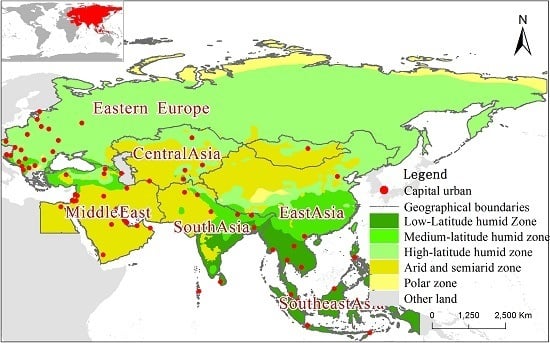
2.1. Study Area and the Divisions of Cities in Different Regions
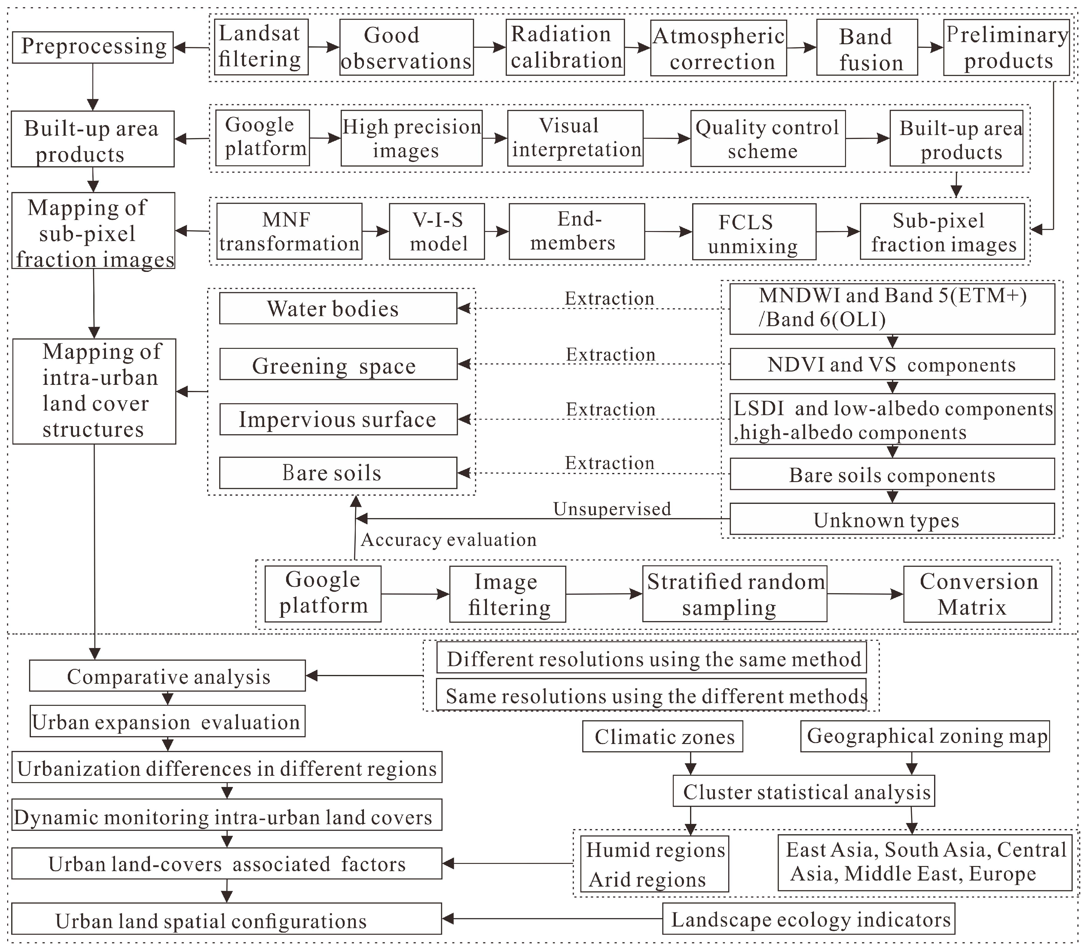
The “Global Belt and Road” is composed of the Belt and the Road within the area between 12°13′24″–180°00′00″E and 9°57′59″–83°05′34″N. The “Global Belt and Road” spans a total of 65 countries with 29.26% of the world’s terrestrial land (i.e., 4.36 × 10⁷ km2) according to the borders as defined from the National Development and Reform Commission of China. The “Belt” (Figure 1, dark red line) links the land areas stretching from China to Africa through the East Asia region, South Asia region, Central Asia region, Eastern Europe region, and Middle East region. The “Road” (Figure 1, dark blue line) stretches marine areas from the east coast of China to the Mediterranean Sea through the South China Sea region, Southeast Asia region, Indian Ocean region and Persian Gulf region. The Belt and Road are also situated across many climatic zones, such as tropical zones, arid zones, humid zones, cold zones, and polar zones according to the updated Köppen–Geiger climate map of the world [34]. The complex terrain covers plateaus, plains, mountains, hills, and basins. Capital cities play the role of the national administrative center in each country [35]. It attracts more people to live in and achieves rapid economic development. The land-cover patterns in the capital cities always change dramatically, either by increasing the percentage of the filling of ISA within the already built-up areas or continuous expansion beyond the urban boundary. Monitoring land-covers and associated changes across all the capital cities provides a potential avenue for research on urbanization processes and intra-urban land structure changes over the Global Belt and Road, and a total of 65 capital cities were selected in the study.
The spatial distribution of the different cities in the study area was determined based on geographical zones from the resource and environment data cloud platforms of China, namely, Central Asia (5 cities), South Asia (8 cities), East Asia (13 cities), the Middle East (19 cities), and Europe (20 cities). The cities in different geographical zones across the 65 countries along the Belt and Road are shown in Table 1.

2.2. Methods

The synergistic intra-urban land-cover classification methodology of SMDU was created (Figure 2). First, all good-observation Landsat images were filtered from June to September during the period 2000–2015. The Landsat Enhanced Thematic Mapper Plus (ETM)+ and Operational Land Imager (OLI) images were processed to generate a 15 m preliminary product. A detailed description can be found in Section 2.2.1. Then, the vegetation-impervious surface-soil (V-I-S) model discriminated four optimal end-member objects, including bare soil object, vegetation object, low-albedo object, and high-albedo object. These four optimized end-member objects were put into the fully constrained least-squares solution model in order to generate four sub-pixel land-cover component images, namely, bare soil component, vegetation component, low-albedo component, and high-albedo component. The sub-pixel land-cover component images within cities were further acquired by overlying built-up areas. The multiple indices and decision tree classifier generated the majority of land-cover classification types. The remaining “unknown urban types” were further identified through unsupervised classification. All steps in this methodology were calculated according to the raster layers. A random stratified sampling (pixels) scheme was applied to quantify the accuracy assessment from historical archived Google Earth imagery. Then, the 15 m resolution urban land-cover product (i.e., the impervious surface area, vegetation, bare soil, and water bodies) across 65 capital cities along the Global Belt and Road was generated.

2.2.1. Data Collection and Pre-Processing

The free availability of Landsat images enables us to achieve large-scale urban land-cover maps. The extraction of high-quality observations from Landsat images was not always available in each month due to the presence of snow cover, clouds, and bad pixel strips [36]. Image information was then filtered to obtain high-quality observations between June and September. During this period, the vegetation and bare soil coverages could be easily identified in built-up areas. A total of 184 high-quality observations from Landsat 7 ETM+ and 179 high-quality observations from Landsat OLI 8 derived from the United States Geological Survey (i.e., USGS; Website: https://www.usgs.gov/) were obtained. Fine resolution obtained from the remotely sensed images can better represent the detailed spatial land-cover patterns [37], especially for complex arrangements of land-cover types in urban landscapes. Gram–Schmidt spectral sharpening has been shown to be an effective data fusion method for integrating the 30 m multispectral band and the 15 m panchromatic band so as to obtain the new 15 m Landsat data using the high-quality observations from the Landsat ETM+/OLI images [38,39]. Thus, this technique was used in this research. The Fast Line-of-sight Atmospheric Analysis Spectral Hypercubes (FLAASH) was used to conduct the atmospheric calibration. The Fast Line-of-sight Atmospheric Analysis Spectral Hypercubes is a first-principles atmospheric calibration tool that corrected wavelengths in the visible through near-infrared and shortwave infrared regions. Unlike many other atmospheric correction programs that interpolate radiation transfer properties from a pre-calculated database of modelling results, FLAASH incorporated the moderate resolution atmospheric transmission 4 (MODTRAN4) radiation transfer code. The version of MODTRAN4 incorporated into ENVI FLAASH was modified to correct errors in the HITRAN-96 water line parameters [40]. Therefore, ENVI FLAASH is suitable for use with multispectral sensors (such as those onboard the Landsat satellites) and can correct images collected in either vertical (nadir) or slant-viewing geometries [41]. These images were also pre-processed through radiometric calibration from the ENVI platform and re-projection from the ARCGIS platform.

2.2.2. Built-Up Area Extraction

To obtain the spatial extent of built-up areas, the main technical method was composed of the following steps: built-up area definition, 2 m Google image download, artificially digitized interaction, and data quality control scheme. Currently, various built-up area definitions exist in the literature. From the land-cover perspective, the popular definition refers to built-up area as artificial impervious surfaces such as buildings, squares, pavements, and bricks [42,43], while this definition results in the built-up area discontinuity due to the lack of non-artificial land-covers. In the study, the built-up areas should contain artificial impervious surfaces and non-artificial land types (i.e., water bodies, bare soil, and vegetation) within the artificially digitized boundaries from 2 m Google images. The Google Earth platform provides a convenient way of obtaining the historical imagery archive for the years of 2000 and 2015. All images were downloaded through professionally authorized payment software (i.e., 91 bitmap platform, http://www.91weitu.com/). The former built-up area layer (shapefile format) was a visual human–computer interpretation according to professional knowledge through land features in 2 m Google images in 2000. After that, the resulting layer was overlaid onto the Google Earth images in 2015 to generate the later built-up areas. During this process, a data quality control scheme was implemented because the results of artificial visual interpretation relied on the expertise of individuals. All built-up areas were repeatedly interpreted by different individuals to correct the misinformation. The vector layers of the built-up areas in 2000 and 2015 were obtained and further converted into 15 m resolution raster data layers. The spatial extent of the 65 capital cities in 2000 and 2015 was generated.

2.2.3. Mapping of Sub-Pixel Urban Land-Cover Components

Many mixed pixels between impervious surface areas and bare soil existed in arid and semi-arid regions of the Global Belt and Road. Previous pixel classification methods were difficult to separate on the pixel-level. In this study, we classified the pixel-level images into four sub-pixel land components. On the sub-pixel level, the combination of sub-pixel land fractions and multiple index was conducted to separate mixed pixels. Decision tree classifier and unsupervised classification were applied to obtain the pixel-level land classification again according to the sub-pixel level data. The synergistic classification methodology of SMDU classification in the study may effectively deal with the mixed pixel issues. Therefore, the sub-pixel urban land-cover components should be firstly obtained. Then, the urban land-cover classification was implemented.
Mapping of sub-pixel urban land-cover components was usually generated through linear spectral mixture analysis (LSMA) technology in the remote sensing literature, while this technique cannot ensure component values ranging from 0 to 1 [44,45]. A fully constrained least-squares solution model (i.e., Equation (1)) [46] can effectively address this issue and transform Landsat images into a linear combination of four sub-pixel land-cover components, namely, bare soil component, vegetation component, low-albedo component, and high-albedo component. Filtering of end-members for each component is the most important step because the spectral features of end-members can significantly affect the accuracy of sub-pixel land-cover components. To obtain the best spectral end-members, minimum noise fraction technology was utilized to transform Landsat ETM+ and OLI bands into a new dataset, in which the first three bands occupied over 90% of the total land-cover spectral information. Subsequently, a vegetation-impervious surface-soil model was applied to identify each end-member and collect these four optimized end-members. Then, a constrained least-squares solution model was applied to generate four land-cover components according to the optimized end-members. Mixed pixel decomposition can be applied to only one image due to the varied spectral features in different built-up areas. Therefore, the new end-members for each image must be re-selected, and a total of 1452 optimized end-members were obtained in the years of 2000 and 2015 over the study area. We repeated the steps to obtain all sub-pixel urban land components according to Landsat ETM+/OLI images.

2.2.4. Mapping of Intra-Urban Land-Cover Classifications

Spectral features and component thresholds of image bands are usually utilized to classify urban land, while mixed pixels affect the intra-urban classification accuracy. Although the images with high-albedo components focused on bright ISA, such as the land-covers at the top of buildings, while bare soil also existed in the high-albedo component images. Meanwhile, images with low-albedo components focused on dark ISA, such as building shadows, while rivers, lakes, and ponds also existed in the low-albedo component images. The misinformation should be eliminated from the images in both high- and low-albedo components. The low-albedo soil difference index (LSDI) (i.e., Equation (2)) [47] can distinguish bare soil from bright ISA in high-albedo images, and the modified normalized difference water index (MNDWI) (i.e., Equation (3)) [48] can distinguish water bodies from dark ISA in low-albedo component images. These two indices were used in this study.
The classification methodology of SMDU classification (SMDU) was established here to distinguish intra-urban land-covers. Namely, the MNDWI and Landsat bands were adopted to obtain the urban water body; NDVI (i.e., Equation (4)) [49] and vegetation component images were adopted to obtain urban greening space (UGS); the LSDI was adopted to distinguish bare soil from impervious land surfaces. After that, although the remaining urban areas (i.e., unknown land-cover types, less than 2.1% in built-up areas based on our study) were limited, they were still mixed urban-land pixels. We further used the unsupervised classification scheme to divide the unknown land-covers. Too many classifications led to large manual workload, while fewer classifications were difficult to meet the high classification accuracy. The test of 50 classified categories in the unknown land-cover areas were suitable that they were grouped into four categories per image. A total of 18,150 categories from 363 Landsat ETM+ and OLI images were identified through manual allocation. Finally, the scattered urban land-covers were integrated into the maps for 2000 and 2015 across 65 countries along the Global Belt and Road.
R i λ = k = 1 n f k i C k λ + ε i λ
In Equation (1), R i λ is the albedo of the pixel i from the band λ ; f k i is the area proportion of the component k on the pixel i ; c k λ is the albedo of the component k from the band λ ; ε i λ is the residual error.
LSDI = f L o w f S o i l
In Equation (2), f l o w is the low-albedo component images; f s o i l is the bare soil component images.
MNDWI = ( ρ g r e e n ρ M I R ) / ( ρ g r e e n + ρ M I R )
In Equation (3), ρ g r e e n is a green band such as ETM+ band 2 and OLI band 3, and ρ M I R is a middle infrared band such as ETM+ band 5 and OLI band 6.
NDVI = ( ρ N I R ρ r e d ) / ( ρ N I R + ρ r e d )
In Equation (4), ρ N I R is a near infrared band such as ETM+ band 4 and OLI band 5, and ρ r e d is a red band such as ETM+ band 3 and OLI band 4.

2.2.5. Accuracy Assessment

Accuracy assessment of the newly developed 15 m urban land-cover product was performed using randomly selected samples (pixels). A total of 37,200 samples were randomly and equally allocated to each of the years in 2000 and 2015. Two hundred random verification samples were obtained for each city. Because the areas of urban land-cover types varied in different years, it was best to use stratified random sampling to randomly select samples for the urban land-cover types within each city. The historical archived Google Earth images (2 m resolution, Quick Bird sensor) were gathered and considered for the validation imagery datasets. To ensure the temporal consistency of Landsat data sources and Google Earth images, we filtered the validation imagery to match the months of the classification imagery. The transition matrices, overall accuracy, producer and user accuracy, and kappa coefficients were used for the accuracy assessment.
Meanwhile, from a methodological standpoint, it was necessary to test the differences in the results considering 15 m and 30 m pixel sizes according to the proposed method in the study. Further, in order to assess the performance of the proposed method, a comparison with the accuracies obtained with the proposed method using the native pixel size of 30 m, as well as with another method using the decision tree classifier was provided. These quantitative comparisons can better understand the actual improvement of the proposed method in the classification issues. The stratified random sampling, transition matrices, overall accuracy, producer accuracy, user accuracy, and kappa coefficients were also conducted for the accuracy assessment.

2.2.6. The Linking Between Urban Land-Cover Changes and Associated Climatic and Geographical Zones

In order to analyze intra-urban land-cover changes under different climatic distribution zones, the cluster statistical analysis was firstly applied to all climatic zones enumerated in Figure 1. We analyzed the characteristics of urban land-cover changes in each climatic zone during the period of 2000–2015. The similar land-use change results occurred in the tropic zone, humid zone, and cold zone, namely, most of the ISA expansion originated from vegetation space. In contrast, land-use change results indicated that the different land changes occurred in arid and semi-arid zones, namely, most of the ISA expansion originated from bare soil (not vegetation space). No city was located in the polar zone, and therefore not selected for study in this section. According to the cluster statistical analysis results, we organized these climate zones into two types: humid region (i.e., the tropic zone, humid zone, and cold zone) and arid region (i.e., the arid and semi-arid zone). Meanwhile, in order to analyze the relationships between urban land-covers and associated geographical zones, the geographical zones from the resource and environment data cloud platforms of China were provided. The cities in different geographical zones across the 65 countries along the Belt and Road are shown in Figure 1 and Table 1, namely, Central Asia (5 cities), South Asia (8 cities), East Asia (13 cities), the Middle East (19 cities), and Europe (20 cities). Cluster statistical analysis was applied to all geographical zones, and we analyzed the characteristics of urban land-cover changes in each geographical zone.
The land-cover changes within capital cities adjacent to China may be firstly affected by the Global Belt and Road initiative due to these initiated projects, such as the extension of highways and railways, buildings, ports, and hydropower stations, that will cover the adjacent capital cities first. This will provide more jobs for workers. Infrastructure upgrading also attracts more people to live in the capital cities adjacent to China. The agglomeration of population in the capital cities inevitably promoted land-cover changes within or beyond the urban boundary. Therefore, we focused on all the capital cities adjacent to China (i.e., the central zones along the Global Belt and Road) to assess land-cover configurations using landscape ecological indicators. Landscape ecological indicators were always used to reflect the characteristics of land-cover configurations. There are many landscape ecological indicators, but the single index cannot comprehensively obtain the urban land spatial features, while multiple indices sometimes contain redundant information. Considering the urban land-covers across the central zones, some landscape ecological indicators were selected. Detailed information of these indicators, such as full name, abbreviation, expression, and the description of land-cover configurations, are provided in Table 2.

3. Results

3.1. Accuracy Assessment

3.1.1. Accuracy Assessment for the New Intra-Urban Land Product

Overall classification accuracy of the 15 m urban land-cover product across 65 capital cities along the Global Belt and Road amounted to 92.88% and 93.19%, with kappa coefficients ranging from 0.842 to 0.855 in 2000 and 2015, respectively (Table 3). Most misclassification information occurred between ISA and bare soil. The misclassification information was reasonable because complicated man-made coverage materials and divergent urban land surface colors resulted in widespread spectral signatures in the ISA; thus, the high-albedo impervious surface had similar spectral signatures with that of bare soil. The study promoted a classification methodology to identify the urban land-cover within built-up areas across 65 capital cities along the Global Belt and Road. The methodology indicated that the intra-urban land classification product had high classification accuracy.

3.1.2. Comparison the Accuracies from Different Classification Resolutions and Methods

The quantitative comparison of the accuracies was conducted to understand the actual improvement of the proposed method in the classification issues considering the mixed pixels. Because the main issues of urban land-cover classification were to separate bare soil and ISA, we chose Toshkent, a typical dryland city with median built-up area and population size among the investigated cities, as an example to compare the accuracies. Firstly, the test of different accuracy results from the native 30 m pixel of Landsat and the downscaled 15 m pixel of urban land-cover product were provided according to the proposed method in the study. Table 4 indicated that the results from 15 m data improved 1.25% of the overall classification accuracy compared to the results from 30 m data, with both the user and producer accuracies of the ISA and soil types being improved by 1.18% and 1.17%, and by 1.67% and 3.93%, respectively. Then, a comparison with the accuracies obtained with the proposed method in the study using the native 30 m pixel of Landsat, as well as with the method of linear spectral mixture analysis and decision tree classifier (LD) were also provided. On the 30 m pixel scale, the proposed method improved 4.75% of the overall classification accuracy compared to the results from the LD method. The user and producer accuracies of the ISA and soil types were also improved by 5.67% and 5.11%, and by 8.15% and 8.37%, respectively. The new features of the proposed methodology with respect to a standard one using the LD method were that the multiple index and unsupervised classification improved the separation between ISA and bare soil.

3.2. Urban Spatial Expansion Discrepancy in Different Regions

The presented urban land product allowed us to describe the characteristics of urbanization in the 21st century within the Global Belt and Road (Figure 3). The analysis of the built-up area data derived from 2 m Google Earth images indicated that the estimated built-up areas were 23,696.25 km2 in 2000 and increased to 29,257.51 km2 in 2015, with a total increase in the urban expansion rate (UR) of 23.47% during the study period. A significant difference in the UR was observed, with the highest UR in South Asia (30.17%) and the lowest in Europe (12.57%). The UR in the other regions followed the order of East Asia (27.53%) > Middle East (22.51%) > Central Asia (22.17%).
Figure 4 presents the top 10 cities with the most rapid urban expansion. Taken together, these 10 cities shared 59.52% of the total increases in urban expansion in 2000–2015. In particular, the top three cities, i.e., Beijing (China), New Deli (India), and Bangkok (Thailand) together (20.56% of the built-up areas in 2000) already contributed 31.68% of the total urban expansion. Overall, these results were important for urban studies, such as the forecast of urban growth in the future and rank-level urban comparison on regional and global scales.

3.3. Intra-Urban Land-Cover Dynamic Changes

The intra-urban land-cover changes within the Global Belt and Road between 2000 and 2015 are presented in Figure 5. Examples of final classified intra-urban land-cover images are provided in Figure 6. Across the 65 capital cities, urban ISA expanded from 13,987.89 km2 (2000) to 20,016.68 km2 (2015), with an average rate of 401.92 km2/yr. There was a loss of UGS from 5830.70 km2 to 5566.85 km2, with an average rate of 17.59 km2/yr in the study period. Similarly, the coverage of urban bare soil decreased from 3399.51 km2 to 3120.99 km2, with an average rate of 18.57 km2/yr. The land cover of neglected urban water bodies remained stable. It was clear from the information that the average loss rates from UGS and urban bare soil were basically the same.

3.4. Analysis of the Linking Between Urban Land-Covers and Associated Climatic and Geographical Regions

For the intra-urban land-cover changes in different climatic regions (Figure 5 and Table 5), the overall cover of ISA increased by 48.43% in humid cities and 42.60% in arid cities. Meanwhile, the overall cover of bare soil declined by 28.09% in humid cities and only by 1.02% in arid cities. A reverse phenomenon was observed for vegetation changes, namely, the vegetation coverage declined by 7.37% in humid cities but increased by 14.61% in arid cities. Therefore, urban vegetation changes exhibited opposite trends in arid and humid cities.
The intra-urban land-cover changes in different geographical regions are provided in Table 5. For urban land-covers in 2015, the proportions of impervious surface coverage to built-up areas are presented in the following order: East Asia (74.56%) > South Asia (73.74%) > Middle East (62.78%) > Central Asia (62.51%) > Europe (61.28%). Meanwhile, the proportions of vegetation followed the following order: Europe (29.62%) > East Asia (20.23%) > South Asia (18.38%) > Central Asia (14.94%) > Middle East (12.18%); in contrast, the proportions of bare soils followed the order of Middle East (23.93%) > Central Asia (21.78%) > South Asia (6.61%) > East Asia (3.97%) > and Europe (3.50%). The urban land dynamic changes in emerging developing country regions showed that pronounced impervious surface expansion had occurred with ISAs increasing from 11,577.36 km2 (2000) to 17,106.16 km2 (2015), which represents an increase of 47.76%. High-density vegetation was observed in traditional developed country regions such as Europe, with vegetation coverage increasing from 32.83% (2000) to 33.35% (2015) within built-up areas. The former underwent rapid impervious surface expansion, while the latter presented comfortable green environments.

3.5. Analysis of the Urban Land Configurations in Central Cities

During 2000–2015, urban land configurations became more integrated (△SHDI = −0.063; △PD = −0.054, Figure 7b). Urbanization presented divergence (△LSI = 0.021, Figure 7b), accompanied by a better connectivity (△CON = +0.594, Figure 7b). Concerning the land-cover types, all urban land types became more fragmented except the ISA (△PD of the ISA = −0.053, Figure 7c). The urbanization process promoted ISA to form centralized patterns (△LPI of the ISA = 0.711, Figure 7d; △CON of the ISA = 0.263, Figure 7e), whereas opposite changes were observed in vegetation and bare soil areas (△PD, △LPI, and △CON of the VS and soil, Figure 7c–e), indicating that their patches became separated from each other because of ever-expanding ISA. An interesting commonality for all intra-urban land-cover types according to the urban ecological indicators showed that the land-cover LSI (i.e., LSI of all the land covers, Figure 7f) became more complex.

4. Discussion

4.1. The First High-Resolution Intra-Urban Land-Cover Mapping Product within the Global Belt and Road

A synergistic classification methodology in this study was created to obtain 15 m intra-urban land-cover product within the Global Belt and Road. Figure 8 shows the comparison of urban land-cover classification results obtained by this methodology and the results from contemporary global products (i.e., global land-cover 30 m, GLC30-m; global human settlement layer 38 m, GHSL 38-m; European space agency global land-cover data 300 m, ESA-GlobCover 300-m; and moderate-resolution imaging spectroradiometer 500 m, MODIS 500-m [13,14,16,51]) in similar epochs. The built-up area in these global products was regarded as impervious surfaces such as buildings, squares, pavements, and bricks, which led to land-cover discontinuity within built-up areas due to the lack of non-artificial land-covers. The built-up area in the study contained impervious surface areas, water bodies, bare soil, and vegetation, and all land-covers within the built-up area were continuous, indicating that the 15 m resolution built-up area product in this study allowed us to display detailed urban land-cover spatial patterns, and therefore, provided essential details for complex urban landscapes and urban ecological needs. Furthermore, these global built-up products were obtained through pixel classification. The proposed method in the study was obtained through the sub-pixel-level and pixel-level classification. On the sub-pixel level, the combination of sub-pixel land fractions and multiple index was conducted to separate mixed pixels. Decision tree classifier and unsupervised classification were applied to obtain the pixel-level land classification again according to the sub-pixel level data. This methodology can improve the separation of mixed pixels. In this study, there were acute land-use changes within built-up areas across 65 capital cities during 2000–2015. These changes most likely represented the general changes in urban land-use worldwide. A significant ISA expansion was observed in the study area, including the extension of highways, railways, buildings, squares, ports, and hydropower stations in urban areas. These changes facilitated the promotion of trade among all countries within the Global Belt and Road. Another finding was that the average loss rates from UGS and urban bare soil were similar. This result was because the study area spans multiple climatic zones, including humid and arid regions [52,53]. The urban land dynamic changes in the humid region indicated that the ISA expansion was mainly attributed to the transformation of vegetation space; in contrast, the arid region was characterized by the transformation of abundant bare soil space into new ISA. In this study, we also found that the proportions of UGS within built-up areas increased in arid cities, which indicated a beneficial effect on the capability of fixing sand and dust [54], and further improving human settlement environments.

4.2. The Impacts of Economic Development and Population Migration on Livable Urban Environments

Urbanization has a profound impact on livable urban environments. This study found that the cities in emerging developing country regions underwent rapid urbanization, such as South Asia (UR: 30.17%) and East Asia (UR: 27.53%). Urbanization in these regions should be of particular concern, as well as the population-driven forces. The focus of global economic development has migrated to these regions and provided many opportunities for people to work in cities [55,56], which promoted large-scale population migration to metropolitan areas. These people prefer to live in metropolitan areas due to their improved human comfortability, such as convenient facilities. Conversely, cities in traditional developed country regions such as Europe have observed the lowest UR (12.57%). The infill densification of already built-up areas may be the main driver of urban land-cover dynamics in traditional developed country regions due to the low population density and the completed population migration from rural areas to cities. The people in these regions may prefer to live in cities with comfortable human settlement environments. The livable small and medium-sized cities probably provided alternative choices to live in instead of metropolitan areas.

4.3. Intensified Interactions between Residential Areas and Existing Green Space

The findings in this study showed that the urbanization process had a significant impact on urban green systems [57], such as vegetation coverage and vegetation fragmentation. For vegetation coverage, the existing vegetation coverage was invaded by an ever-expanding ISA, leading to vegetation patches becoming separated from each other. For the vegetation fragmentation, it can be reflected by the changes in landscape ecological indicators. The increases in PD of vegetation space indicated the increasingly segregated vegetation space. The reductions in LPI of vegetation space indicated the decrease in land-cover dominance. Under the condition of ever-expanding ISA, the interactions between residential areas and vegetation space was improved. More intense interactions can be captured in the regions of East Asia, South Asia, Middle East, and Central Asia due to the large-scale population migration from rural areas to cities. In order to balance the contradiction between large population and limited cropland resources in these regions [58,59,60], urban space control policies usually provided a certain amount of land for urban expansion. As a result, significant amounts of existing green space or vacant land within built-up areas were converted into residential space. This condition will impact the sustainability of vulnerable urban environments in arid cities due to the arid natural environments [61]. A certain amount of vegetation space should be preserved or planted to maintain the human settlement environments and ecosystem services. In the prospect of climate warming and extreme meteorological events, awareness of the incorporation of green systems needs to be triggered as an essential role with strong mutual dependence between rapid economic growth and sustainable urban environments.

4.4. Comparison of Different Environmental Effects in Arid and Humid Regions According to the Intra-Urban Land-Cover Changes

The environmental effects in arid and humid regions according to the intra-urban land-cover changes were notably different. These effects included changes in the natural role of the regional carbon cycle. With rapid urban expansion, ISA carbon sinks were mainly from high-density vegetation carbon sources [62] in humid cities. In contrast, these sources were replaced by low-density bare soil carbon sources in arid cities. Another effect was surface energy. In warm seasons, ISA expansion invaded existing green space and led to increases in the land surface temperature (LST) in humid urbans, namely, the urban heat island (UHI) phenomenon [63]. In arid cities, the albedo of bare soil was lower than that of ISA [64], which caused the bare soil to absorb more energy during the daytime, and thus exhibited increased temperature; ISA expansion invaded bare soil and led to the decreases in LST in arid cities, namely, the opposite of the UHI phenomenon. In cold seasons, the complex interactions between maritime climate and land feedbacks in coastal cities [65] and inhomogeneous snow cover in inland cities increased the complexity of the surface energy. For achieving sustainable urban and environment coordinated development within the Global Belt and Road, the industrial structure and energy distribution patterns in urban areas should be further studied to provide environmental effects on the compositions of pollutants and carbon emissions.

4.5. Study Limitations

Our study focused on all capital cities (a total of 65 cities) along the Belt and Road. The images with the capital cities were downloaded. Due to the spatial distribution discontinuity in these capital cities and the complex spectral characteristics in the study area, the proposed method in the study was conducted to classify images one by one. Finally, the 15 m resolution built-up area product (i.e., the impervious surface area, vegetation, bare soil, and water bodies) across the 65 capital cities along the Belt and Road was obtained. For this method, the filtering of end-members for each land-cover component was the most important step because the spectral features of end-members can significantly affect the accuracy of sub-pixel land-cover components. It is difficult to find the universal end-members on a large scale due to the complex spectral characteristics of land-covers. In order to monitor land use and land-cover changes over a broad scale, the filtering of universal end-members in this method will be further studied.

5. Conclusions

The overarching objective in this study was to conduct city-level comparisons of urban land-cover changes in 2000–2015 across 65 countries within the Global Belt and Road. To meet this goal, the synergistic classification methodology was created to obtain an urban land-cover classification product derived from remotely sensed satellite images. An accuracy assessment for the new 15 m urban land product exceeded 92% in both 2000 and 2015. Across the 65 cities, the built-up areas increased with an average growth rate of 370.75 km2/yr in 2000–2015. Furthermore, the ISA expanded with an average rate of 401.92 km2/yr, while the total areas of UGS and UBS decreased with equal average rates. In different regions, UGS changes exhibited opposite trends in arid and humid cities. According to the landscape ecology indicators, urban land-cover configurations became more integrated and presented better connectivity. The proposed method in the study improved the separation of mixed pixels between ISA and bare soil, and the first 15 m resolution urban land mapping product across 65 capital cities within the global Belt and Road in this study allowed us to provide essential details for complex urban landscapes and urban ecological security compared to other contemporary global products. These results provided significant information on the sustainability of the Global Belt and Road and provided important knowledge to understand the effect of intra-urban land-cover changes regarding livable urban environments and urban ecological security.

Author Contributions

Conceptualization, W.K.; Data curation, C.Z. and T.P.; Methodology, C.Z. and T.P.; Visualization, W.K.; Writing—original draft, C.Z. and T.P.; Writing—review & editing, W.K., R.H., C.Z., T.P., S.Z., Z.L. and X.C.

Funding

The study was supported by the Strategic Priority Research Program of Chinese Academy of Sciences, Pan-Third Pole Environment Study for a Green Silk Road (Pan-TPE) (NO: XDA20040400); Chi Zhang is supported by the Taishan Scholars Program of Shandong, China, Grant No. ts201712071; and Tao Pan is supported by the Open Fund of Shandong Provincial Key Laboratory of Water and Soil Conservation and Environmental Protection, China, Grant No. STKF201937; Chi Zhang, Tao Pan, and Xi Chen’s works were supported by the Research Center for Ecology and Environment of Central Asia, Chinese Academy of Sciences, Urumqi 830011China.

Acknowledgments

We thank the academic editor and reviewers for their constructive comments which greatly helped us to improve the quality of this manuscript.

Conflicts of Interest

The authors declare no conflict of interest. The founding sponsors had no role in the design of the study, in the collection, analyses, or interpretation of the data, in the writing of the manuscript, or in the decision to publish the results.

References

  1. Kamali, M.; Delkash, M.; Tajrishy, M. Evaluation of permeable pavement responses to urban surface runoff. J. Environ. Manag. 2017, 187, 43–53. [Google Scholar] [CrossRef] [PubMed]
  2. Yin, J.; Xu, S.; Wen, J. Community-based scenario modelling and disaster risk assessment of urban rainstorm waterlogging. J. Geogr. Sci. 2011, 21, 274–284. [Google Scholar] [CrossRef]
  3. Clinton, N.; Gong, P. MODIS detected surface urban heat islands and sinks: Global locations and controls. Remote Sens. Environ. 2013, 134, 294–304. [Google Scholar] [CrossRef]
  4. Wang, S.; Fang, C.; Wang, Y.; Huang, Y.; Ma, H. Quantifying the relationship between urban development intensity and carbon dioxide emissions using a panel data analysis. Ecol. Indic. 2015, 49, 121–131. [Google Scholar] [CrossRef]
  5. Lutz, W.; Sanderson, W.; Scherbov, S. The end of world population growth. Nature 2001, 412, 543–545. [Google Scholar] [CrossRef] [PubMed] [Green Version]
  6. Glaeser, E.L.; Kerr, S.P.; Kerr, W.R. Entrepreneurship and Urban Growth: An Empirical Assessment with Historical Mines. Rev. Econ. Stat. 2015, 97, 498–520. [Google Scholar] [CrossRef]
  7. Seto, K.C.; Güneralp, B.; Hutyra, L.R. Global forecasts of urban expansion to 2030 and direct impacts on biodiversity and carbon pools. Proc. Natl. Acad. Sci. USA 2012, 109, 16083–16088. [Google Scholar] [CrossRef] [Green Version]
  8. Solecki, W.; Seto, K.C.; Marcotullio, P.J. It’s time for an urbanization science. Environ. Sci. Policy Sustain. Dev. 2013, 55, 12–17. [Google Scholar] [CrossRef]
  9. Dong, J.; Kuang, W.; Liu, J. Continuous land cover change monitoring in the remote sensing big data era. Sci. China Earth Sci. 2017, 60, 2223–2224. [Google Scholar] [CrossRef]
  10. Ahern, J. From fail-safe to safe-to-fail: Sustainability and resilience in the new urban world. Landsc. Urban Plan. 2011, 100, 341–343. [Google Scholar] [CrossRef] [Green Version]
  11. Santé, I.; García, A.M.; Miranda, D.; Crecente, R. Cellular automata models for the simulation of real-world urban processes: A review and analysis. Landsc. Urban Plan. 2010, 96, 108–122. [Google Scholar] [CrossRef]
  12. Kuang, W.; Yang, T.; Yan, F. Examining urban land-cover characteristics and ecological regulation during the construction of Xiong’an New District, Hebei Province, China. J. Geogr. Sci. 2018, 28, 109–123. [Google Scholar] [CrossRef]
  13. Friedl, M.A.; McIver, D.K.; Hodges, J.C.; Zhang, X.; Muchoney, D.; Strahler, A.H.; Woodcock, C.E.; Gopal, S.; Schneider, A.; Cooper, A.; et al. Global land cover mapping from MODIS: Algorithms and early results. Remote Sens. Environ. 2002, 83, 287–302. [Google Scholar] [CrossRef]
  14. Hollmann, R.; Merchant, C.J.; Saunders, R.; Downy, C.; Buchwitz, M.; Cazenave, A.; Chuvieco, E.; Defourny, P.; de Leeuw, G.; Forsberg, R.; et al. The ESA climate change initiative: Satellite data records for essential climate variables. Bull. Am. Meteorol. Soc. 2013, 94, 1541–1552. [Google Scholar] [CrossRef]
  15. Zhang, Z.; Wang, X.; Zhao, X.; Liu, B.; Yi, L.; Zuo, L.; Wen, Q.; Liu, F.; Xu, J.; Hu, S.; et al. A 2010 update of National Land Use/Cover Database of China at 1:100000 scale using medium spatial resolution satellite images. Remote Sens. Environ. 2014, 149, 142–154. [Google Scholar] [CrossRef]
  16. Ning, J.; Liu, J.; Kuang, W.; Xu, X.; Zhang, S.; Yan, C.; Li, R.; Wu, S.; Hu, Y.; Du, G.; et al. Spatiotemporal patterns and characteristics of land-use change in China during 2010–2015. J. Geogr. Sci. 2018, 28, 547–562. [Google Scholar] [CrossRef]
  17. Yu, L.; Liu, X.; Zhao, Y.; Yu, C.; Gong, P. Difficult to map regions in 30 m global land cover mapping determined with a common validation dataset. Int. J. Remote Sens. 2018, 39, 4077–4087. [Google Scholar] [CrossRef]
  18. Chen, J.; Chen, J.; Liao, A.; Cao, X.; Chen, L.; Chen, X.; He, C.; Han, G.; Peng, S.; Lu, M.; et al. Global land cover mapping at 30 m resolution: A POK-based operational approach. ISPRS J. Photogramm. Remote Sens. 2015, 103, 7–27. [Google Scholar] [CrossRef]
  19. Liu, X.; Hu, G.; Ai, B.; Li, X.; Shi, Q. A normalized urban area composite index (NUACI) based on combination of DMSP-OLS and MODIS for mapping impervious surface area. Remote Sens. 2015, 7, 17168–17189. [Google Scholar] [CrossRef]
  20. Li, P.; Qian, H.; Howard, K.W.; Wu, J. Building a new and sustainable “Silk Road economic belt”. Environ. Earth Sci. 2015, 74, 7267–7270. [Google Scholar] [CrossRef]
  21. Szczudlik-Tatar, J. China’s New Silk road diplomacy. Policy Pap. 2013, 34. Available online: https://www.files.ethz.ch/isn/174833/PISM%20Policy%20Paper%20no%2034%20(82).pdf (accessed on 25 June 2019).
  22. Tracy, E.F.; Shvarts, E.; Simonov, E.; Babenko, M. China’s new Eurasian ambitions: The environmental risks of the Silk Road Economic Belt. Eurasian Geogr. Econ. 2017, 58, 56–88. [Google Scholar] [CrossRef]
  23. Howard, K.W.; Howard, K.K. The new “Silk Road Economic Belt” as a threat to the sustainable management of Central Asia’s transboundary water resources. Environ. Earth Sci. 2016, 75, 976. [Google Scholar] [CrossRef]
  24. Li, P.; Qian, H.; Zhou, W. Finding harmony between the environment and humanity: An introduction to the thematic issue of the Silk Road. Environ. Earth Sci. 2017, 76, 105. [Google Scholar] [CrossRef]
  25. Lin, M.-L.; Chen, C.-W. Application of fuzzy models for the monitoring of ecologically sensitive ecosystems in a dynamic semi-arid landscape from satellite imagery. Eng. Comput. 2010, 27, 5–19. [Google Scholar] [CrossRef]
  26. Huang, J.; Ji, M.; Xie, Y.; Wang, S.; He, Y.; Ran, J. Global semi-arid climate change over last 60 years. Clim. Dyn. 2016, 46, 1131–1150. [Google Scholar] [CrossRef]
  27. Ammar, A.; Riksen, M.; Ouessar, M.; Ritsema, C. Identification of suitable sites for rainwater harvesting structures in arid and semi-arid regions: A review. Int. Soil Water Conserv. Res. 2016, 4, 108–120. [Google Scholar] [CrossRef] [Green Version]
  28. O’Farrell, P.; Reyers, B.; Le Maitre, D.C.; Milton, S.; Egoh, B.; Maherry, A.; Colvin, C.; Atkinson, D.; De Lange, W.; Blignaut, J. Multi-functional landscapes in semi-arid environments: Implications for biodiversity and ecosystem services. Landsc. Ecol. 2010, 25, 1231–1246. [Google Scholar] [CrossRef]
  29. Huang, J.; Yu, H.; Guan, X.; Wang, G.; Guo, R. Accelerated dryland expansion under climate change. Nat. Clim. Chang. 2016, 6, 166–171. [Google Scholar] [CrossRef]
  30. Eliasson, J. The rising pressure of global water shortages. Nat. News 2015, 517, 6. [Google Scholar] [CrossRef]
  31. Ahmad, A.; Quegan, S. Analysis of maximum likelihood classification on multispectral data. Appl. Math. Sci. 2012, 6, 6425–6436. [Google Scholar]
  32. Okujeni, A.; van der Linden, S.; Hostert, P. Extending the vegetation–impervious–soil model using simulated EnMAP data and machine learning. Remote Sens. Environ. 2015, 158, 69–80. [Google Scholar] [CrossRef]
  33. Wang, J.; Wu, Z.; Wu, C.; Cao, Z.; Fan, W.; Tarolli, P. Improving impervious surface estimation: An integrated method of classification and regression trees (CART) and linear spectral mixture analysis (LSMA) based on error analysis. GISci. Remote Sens. 2018, 55, 583–603. [Google Scholar] [CrossRef]
  34. Beck, H.E.; Zimmermann, N.E.; McVicar, T.R.; Vergopolan, N.; Berg, A.; Wood, E.F. Present and future Köppen-Geiger climate classification maps at 1-km resolution. Sci. Data 2018, 5, 180214. [Google Scholar] [CrossRef] [PubMed]
  35. Kaufmann, D.; Sager, F. How to organize secondary capital city regions: Institutional drivers of locational policy coordination. Governance 2019, 32, 63–81. [Google Scholar] [CrossRef]
  36. Lu, D.; Moran, E.; Hetrick, S. Detection of impervious surface change with multitemporal Landsat images in an urban-rural frontier. ISPRS J. Photogramm. Remote Sens. 2011, 66, 298–306. [Google Scholar] [CrossRef] [PubMed]
  37. Lu, D.; Li, G.; Kuang, W.; Moran, E. Methods to extract impervious surface areas from satellite images. Int. J. Digit. Earth 2013, 7, 93–112. [Google Scholar] [CrossRef]
  38. Feng, Y.; Lu, D.; Moran, E.; Dutra, L.; Calvi, M.; de Oliveira, M. Examining Spatial Distribution and Dynamic Change of Urban Land Covers in the Brazilian Amazon Using Multitemporal Multisensor High Spatial Resolution Satellite Imagery. Remote Sens. 2017, 9, 381. [Google Scholar] [CrossRef]
  39. Ehlers, M.; Klonus, S.; Johan Åstrand, P.; Rosso, P. Multi-sensor image fusion for pansharpening in remote sensing. Int. J. Image Data Fusion 2010, 1, 25–45. [Google Scholar] [CrossRef]
  40. Flaash, U.S.G. Atmospheric Correction Module: QUAC and Flaash User Guide v. 4; ITT Visual Information Solutions Inc.: Boulder, CO, USA, 2009. [Google Scholar]
  41. Bernstein, L.; Adler-Golden, S.; Sundberg, R.; Ratkowski, A. Improved reflectance retrieval from hyper-and multispectral imagery without prior scene or sensor information. In Remote Sensing of Clouds and the Atmosphere XI; International Society for Optics and Photonics: Bellingham, WA, USA, 2006; Volume 63622. [Google Scholar]
  42. Liu, X.; Hu, G.; Chen, Y.; Li, X.; Xu, X.; Li, S.; Pei, F.; Wang, S. High-resolution multi-temporal mapping of global urban land using Landsat images based on the Google Earth Engine Platform. Remote Sens. Environ. 2018, 209, 227–239. [Google Scholar] [CrossRef]
  43. Kuang, W.; Chen, L.; Liu, J.; Xiang, W.; Chi, W.; Lu, D.; Yang, T.; Pan, T.; Liu, A. Remote sensing-based artificial surface cover classification in Asia and spatial pattern analysis. Sci. China Earth Sci. 2016, 59, 1720–1737. [Google Scholar] [CrossRef]
  44. Fan, F.; Fan, W.; Weng, Q. Improving urban impervious surface mapping by linear spectral mixture analysis and using spectral indices. Can. J. Remote Sens. 2015, 41, 577–586. [Google Scholar] [CrossRef]
  45. Lu, D.; Weng, Q. Use of impervious surface in urban land-use classification. Remote Sens. Environ. 2006, 102, 146–160. [Google Scholar] [CrossRef]
  46. Wilson, M.; Reynolds, G.; Kauppinen, R.A.; Arvanitis, T.N.; Peet, A.C. A constrained least-squares approach to the automated quantitation of in vivo (1) H magnetic resonance spectroscopy data. Magn. Reson. Med. 2011, 65, 1–12. [Google Scholar] [CrossRef] [PubMed]
  47. Zhang, C.; Chen, Y.; Lu, D. Mapping the land-cover distribution in arid and semiarid urban landscapes with Landsat Thematic Mapper imagery. Int. J. Remote Sens. 2015, 36, 4483–4500. [Google Scholar] [CrossRef]
  48. Xu, H. Modification of normalised difference water index (NDWI) to enhance open water features in remotely sensed imagery. Int. J. Remote Sens. 2006, 27, 3025–3033. [Google Scholar] [CrossRef]
  49. Tucker, C.J. Red and photographic infrared linear combinations for monitoring vegetation. Remote Sens. Environ. 1979, 8, 127–150. [Google Scholar] [CrossRef] [Green Version]
  50. McGarigal, K.; Cushman, S.A.; Ene, E. FRAGSTATS v4: Spatial Pattern Analysis Program for Categorical and Continuous Maps. Computer Software Program Produced by the Authors at the University of Massachusetts, Amherst. Available online: http://www. umass. edu/landeco/research/fragstats/fragstats (accessed on 26 June 2012).
  51. Pesaresi, M.; Ehrlich, D.; Ferri, S.; Florczyk, A.; Freire, S.; Halkia, M.; Julea, A.; Kemper, T.; Soille, P.; Syrris, V.; et al. Operating Procedure for the Production of the Global Human Settlement Layer from Landsat Data of the Epochs 1975, 1990, 2000, and 2014; Publications Office of the European Union: Luxembourg, 2016; pp. 1–62. [Google Scholar]
  52. Tang, K.; Li, Z.; Li, W.; Chen, L. China’s Silk Road and global health. Lancet 2017, 390, 2595–2601. [Google Scholar] [CrossRef]
  53. Zhang, K. Right to Information about, and Involvement in, Environmental Decision Making along the Silk Road Economic Belt. Chin. J. Comp. Law 2017, 5, 58–78. [Google Scholar] [CrossRef] [Green Version]
  54. Yan, Y.; Kuang, W.; Zhang, C.; Chen, C. Impacts of impervious surface expansion on soil organic carbon—A spatially explicit study. Sci. Rep. 2015, 5, 17905. [Google Scholar] [CrossRef]
  55. Chaponnière, J.-R.; Cling, J.-P.; Zhou, B. Vietnam Following in China’S Footsteps: the Third Wave of Emerging Asian Economies; UNU-WIDER: Helsinki, Finland, 2010; p. 26. ISBN 9789292301385. [Google Scholar]
  56. Peng, I.; Wong, J. East Asia. In The Oxford Handbook of the Welfare State; OUP: Oxford, UK, 2010. [Google Scholar]
  57. Nagendra, H.; Nagendran, S.; Paul, S.; Pareeth, S. Graying, greening and fragmentation in the rapidly expanding Indian city of Bangalore. Landsc. Urban Plan. 2012, 105, 400–406. [Google Scholar] [CrossRef]
  58. Rasul, G. Food, water, and energy security in South Asia: A nexus perspective from the Hindu Kush Himalayan region. Environ. Sci. Policy 2014, 39, 35–48. [Google Scholar] [CrossRef]
  59. Nath, R.; Luan, Y.; Yang, W.; Yang, C.; Chen, W.; Li, Q.; Cui, X. Changes in arable land demand for food in India and China: A potential threat to food security. Sustainability 2015, 7, 5371–5397. [Google Scholar] [CrossRef]
  60. Thornton, P.K.; Kristjanson, P.; Förch, W.; Barahona, C.; Cramer, L.; Pradhan, S. Is agricultural adaptation to global change in lower-income countries on track to meet the future food production challenge? Glob. Environ. Chang. 2018, 52, 37–48. [Google Scholar] [CrossRef]
  61. Xu, K.; Yang, D.; Yang, H.; Li, Z.; Qin, Y.; Shen, Y. Spatio-temporal variation of drought in China during 1961–2012: A climatic perspective. J. Hydrol. 2015, 526, 253–264. [Google Scholar] [CrossRef]
  62. Zhang, W.; Huang, B.; Luo, D. Effects of land use and transportation on carbon sources and carbon sinks: A case study in Shenzhen, China. Landsc. Urban Plan. 2014, 122, 175–185. [Google Scholar] [CrossRef]
  63. Tan, Z.; Lau, K.K.-L.; Ng, E. Urban tree design approaches for mitigating daytime urban heat island effects in a high-density urban environment. Energy Build. 2016, 114, 265–274. [Google Scholar] [CrossRef]
  64. Lazzarini, M.; Marpu, P.R.; Ghedira, H. Temperature-land cover interactions: The inversion of urban heat island phenomenon in desert city areas. Remote Sens. Environ. 2013, 130, 136–152. [Google Scholar] [CrossRef]
  65. Poortinga, W.; Whitmarsh, L.; Steg, L.; Böhm, G.; Fisher, S. Climate change perceptions and their individual-level determinants: A cross-European analysis. Glob. Environ. Chang. 2019, 55, 25–35. [Google Scholar] [CrossRef]
Figure 1. Location of the “Global Belt and Road” and associated geographical information.
Remotesensing 11 01515 g001
Figure 2. Technological process of the sub-pixel un-mixing, multiple indices, decision tree classifier, unsupervised classification (SMDU) methodology. Abbreviations: MNF, minimum noise fraction; V-I-S, vegetation-impervious surface-soil; FCLS: fully constrained least-squares solution model; LSDI, low-albedo soil difference index; VS, vegetation space; NDVI, normalized difference vegetation index; MNDWI: modified normalized difference water index.
Remotesensing 11 01515 g002
Figure 3. Urban spatial expansion in each city for the years 2000 and 2015 along the Belt and Road. Notes: The height of the column represents the area of the built-up region in each city.
Remotesensing 11 01515 g003
Figure 4. The top 10 cities with the most rapid urban land expansion during 2000–2015 along the Belt and Road, including the current built-up areas (km2) and built-up area changes (km2). Abbreviations: BEI, Beijing, China; BAN, Bangkok, Thailand; KUA, Kuala Lumpur, Malaysia; JAK, Jakarta, Indonesia; NEW, New_Deli, India; ABU, Abu Dhabi, United Arab Emirates; ANK, Ankara, Turkey; DHA, Dhaka, Bangladesh; DOH, Doha, Qatar; COL, Colombo, Sri Lanka.
Remotesensing 11 01515 g004
Figure 5. Intra-urban land-cover changes in 2000 (a) and 2015 (b) within the Global Belt and Road. Abbreviations: ISA, impervious surface area; UGS: urban green space; UBS: urban bare soil; UWB: urban water body. The circle size represents the built-up area in each capital city.
Remotesensing 11 01515 g005
Figure 6. Examples of final classified intra-urban land-cover images. Notes: The description of the selected cities are as follows in the Figure 6. Kuala Lumpur, Malaysia, East Asia, coastal city, humid region; Dhaka, Bangladesh, South Asia, inland city, humid region; Astana, Kazakhstan; Central Asia, inland city with adequate surface water resources, arid region; Tehran, Iran, Middle East, inland city, arid region; Dushanbe, Tajikistan, and Bishkek, Kyrgyzstan, Central Asia, inland city, arid region.
Remotesensing 11 01515 g006
Figure 7. Urban landscape index features between 2000 and 2015 in the central zones. (a) Spatial distribution of the central zones within the Global Belt and Road; (b) for the landscape scale indicator, the values of PD, LPI, LSI, CON, and SHDI; (c) for the class scale indicator: the values of PD; (d) for the class scale indicator: the values of LPI; (e) for the class scale indicator: the values of CON; and (f) for the class scale indicator: the values of LSI. Abbreviations: PD: patch density; LPI: largest patch index; LSI, landscape shape index; CON: connectance index; SHDI: Shannon’s diversity index.
Remotesensing 11 01515 g007
Figure 8. Comparison of the urban land-cover classification results (i.e., urban land 15 m product in the epoch of 2000) obtained by this methodology and results from contemporary global products (i.e., global land-cover 30 m in the epoch of 2000, GLC 30 m; global human settlement layer 38 m in the epoch of 2000, GHSL 38 m; European space agency global land-cover data 300 m in the epoch of 2000, ESA-GlobCover 300 m; and moderate-resolution imaging spectroradiometer 500 m in the epoch of 2001, MODIS 500 m).
Remotesensing 11 01515 g008
Table 1. The cities in different geographical zones across the 65 countries along the Belt and Road.
DivisionsCity (abbreviation), Country
Central Asia
(5 cities)
Ashgabat (ASH), Turkmenistan; Astana (AST), Kazakhstan; Bishkek (BIS), Kyrgyzstan; Dushanbe (DUS), Tajikistan; Toshkent (TOS), Uzbekistan;
South Asia
(8 cities)
Colombo (COL), Sri Lanka; Dhaka (DHA), Bangladesh; Kabul (KAB), Afghanistan; Kathmandu (KAT), Nepal; Male (MAL), Maldives; New Deli (NEW), India; Islamabad (ISL), Pakistan; Thimphu (THI), Bhutan;
East Asia
(13 cities)
Bangkok (BAN), Thailand; Beijing (BEI), China; Bandar_Seri_Begawan (BSB), Brunei; Dili (DIL), East Timor; Hanoi (HAN), Vietnam; Jakarta (JAK), Indonesia; Kuala Lumpur (KUA), Malaysia; Manila (MAN), Philippines; Naypyidaw (NAY), Myanmar; Phnom_Penh (PHN), Cambodia; Singapore (SIN), Singapore; Ulaanbaatar (ULA), Mongolia; Vientiane (VIE), Laos;
Middle East
(19 cities)
Abu_Dhabi (ABU), United Arab Emirates; Amman (AMM), Jordan; Ankara (ANK), Turkey; Baku (BAK), Azerbaijan; Baghdad (BAQ), Iraq; Beirut (BEIR), Lebanon; Cairo (CAR), Egypt; Damascus (DAM), Syria; Doha (DOH), Qatar; Jerusalem (JER), Palestina;
Kuwait (KUW), Kuwait; Manama (MAN), Bahrain; Muscat (MUS), Oman; Riyadh (RIY), Saudi Arabia; Sanaa (SAN), Yemen; Tbilisi (TBI), Georgia; Teheran (TEH), Iran; Tel_Aviv (TEL), Israel; Yerevan (YER), Armenia;
Europe
(20 cities)
Belgrade (BELG), Serbia; Bratislava (BRA), Slovakia; Budapest (BUD), Hungary; Bucharest (BUC), Romania; Chisinau (CHI), Moldova; Kyiv (KYI), Ukraine; Ljubljana (LJU), Slovenia; Minsk (MIN), Belarus; Moscow (MOS), Russia; Podgorica (POD), Montenegro; Prague (PRA), Czech Republic; Riga (RIG), Latvia; Sarajevo (SAR), Bosnia and Herzegovina; Skopje (SKO), Macedonia; Sofia (SOF), Bulgaria; Tallinn (TAL), Estonia; Tirana (TIR), Albania; Vilnius (VIL), Lithuania; Warsaw (WAR), Poland; Zagreb (ZAG), Croatia;
Table 2. Detailed information regarding landscape ecological indicators [50].
Full NameAbbreviationExpressionDescription of Land-Cover Configurations
Patch DensityPD P D = n i A ( 10 , 000 ) ( 100 )
n i : number of patches of type i
A = total landscape area (m2)
Indicating the number of patches per unit area and providing comparisons in landscape sizes. It is an indicator of land-cover landscape ecological sensitivity.
Largest Patch IndexLPI L P I = max j = 1 n ( a i j ) A ( 100 )
a i j = area (m2) of patch ij
A = total landscape area (m2)
Largest patch index at the class level quantifies the percentage of total landscape area comprised by the largest patch. The simple measure regarding dominance among all the land covers.
Landscape Shape IndexLSI L S I = 0.25 k = 1 m e i k * A o r = 0.25 E * A
E * or e i k * = total length (m) of edge
A = total landscape area (m2)
Standardized measures of total edge or edge density, which can be adjusted according to the size of the landscape. The expression on the left is for the class level and the right one is for horizontal level.
Connectance IndexCON c o n n e c t = [ j k n c i j k n i ( n i 1 ) 2 ] ( 100 )
cijk = joining (or contiguity) between patches j and k (0 = unjoined, 1 = joined) of the corresponding patch type (i).
ni = number of patches in the landscape (class)
Indicating the percentage of maximum possible connections among the land patches. It is an indicator of land-cover landscape ecological sensitivity.
Shannon’s Diversity IndexSHDI S H D I = i = 1 m P i I n ( P i )
P i = proportion of the landscape occupied by patch type (class) i
The measure of diversity in community ecology. Here, it was used in urban landscape.
Table 3. Transition matrices of intra-urban land-cover validation among all capital cities within the Global Belt and Road in the years of 2000 and 2015. The producer and user accuracy, kappa coefficients, and overall accuracy are also provided.
Ground Truth Samples (Pixels)Reference SamplesClassified SamplesNumber CorrectProducer AccuracyUser Accuracy
Land-CoverISAUGBUBSUWB
ISA4676673653951925147467690.06%90.85%
UGB1156573822467896794657396.82%96.75%
UBS38312642373347324779423789.54%88.66%
UWB182348179118871880179194.91%95.27%
Year: 2000, Overall Classification Accuracy = 92.88% (i.e., 17, 277/18, 600), Overall Kappa Statistics = 0.842
ISA64171123162169866866641791.86%93.46%
UGS744708891649114887470895.87%96.34%
UBS4778241242745554710412490.54%87.56%
UWB18926208421482137208497.02%97.52%
Year: 2015, Overall Classification Accuracy = 93.19 % (i.e., 17, 333/18, 600), Overall Kappa Statistics = 0.855
Abbreviations: UWB: urban water body; UBS: urban bare soil; UGS: urban green space; ISA: impervious surface area.
Table 4. Comparison of the accuracies from different classification resolutions and methods. The Toshkent was regarded as an example to compare the accuracies. The transition matrices, producer and user accuracy, kappa coefficients, and overall accuracy are also provided.
Ground Truth Samples (Pixels)Reference SamplesClassified SamplesNumber CorrectProducer AccuracyUser Accuracy
Land-CoverISAUGBUBSUWB
ISA16625117817416693.26%95.40%
UGB31121011511611297.39%96.55%
UBS9179085897992.94%88.76%
UWB0002122212195.45%100.00%
(a) SMDU method: Overall Classification Accuracy = 94.50% (i.e., 378/400), Overall Kappa Statistics = 0.852
ISA16319017717316392.09%94.22%
UGS31061010911010697.25%96.36%
UBS10281091938189.01%87.10%
UWB10023232423100.00%95.83%
(b) SMDU method: Overall Classification Accuracy = 93.25% (i.e., 373/400), Overall Kappa Statistics = 0.854
ISA147116216916614786.98%88.55%
UGS21092011311310996.46%96.46%
UBS17375093957580.65%78.95%
UWB3002325262392.00%88.46%
(c) LD method: Overall Classification Accuracy = 88.50% (i.e., 354/400), Overall Kappa Statistics = 0.839
Notes: (a) Accuracy assessment of the 15 m pixel urban land-cover product according to the proposed method in the study; (b) accuracy assessment of the native 30 m pixel of Landsat according to the proposed method in the study; (c) accuracy assessment of the native 30 m pixel of Landsat according to the linear spectral mixture analysis using the decision tree classifier.
Table 5. Intra-urban land-cover areas (km2) and rates of change (%) in different regions.
Climatic RegionsHumid RegionArid Region
2015 ISA (km2)15,241.124775.57
2015 UGS (km2)4858.58708.28
2015 UBS (km2)1103.822017.17
2015 UWB (km2)469.4383.55
△ ISA (%)+48.43+42.60
△UGS (%)−7.37+14.61
△UBS (%)−28.09−1.02
△UWB (%)−12.85+24.68
Geographical zonesEast AsiaSouth AsiaMiddle EastCentral AsiaEurope
2015 ISA (km2)8596.262464.225169.51876.172910.53
2015 UGS (km2)2332.98614.201003.22209.431407.01
2015 UBS (km2)457.67220.971970.96305.27166.11
2015 UWB (km2)142.6442.2791.0810.87266.13
△ ISA (%)+54.34+50.09+38.93+35.83+20.74
△UGS (%)−13.93−7.28+12.61+15.36+1.57
△UBS (%)−29.01−4.91−3.16−1.85−5.68
△UWB (%)+22.99+38.72+22.35+11.08+7.53
Abbreviations: ISA: impervious surface area; UGS: urban green space; UBS: urban bare soil; UWB: urban water body. The symbol “△” represents the dynamic proportion changes in urban land cover in 2015 compared to that in 2000.

