Determination of Vegetation Thresholds for Assessing Land Use and Land Use Changes in Cambodia using the Google Earth Engine Cloud-Computing Platform

Abstract

As more data and technologies become available, it is important that a simple method is developed for the assessment of land use changes because of the global need to understand the potential climate mitigation that could result from a reduction in deforestation and forest degradation in the tropics. Here, we determined the threshold values of vegetation types to classify land use categories in Cambodia through the analysis of phenological behaviors and the development of a robust phenology-based threshold classification (PBTC) method for the mapping and long-term monitoring of land cover changes. We accessed 2199 Landsat collections using Google Earth Engine (GEE) and applied the Enhanced Vegetation Index (EVI) and harmonic regression methods to identify phenological behaviors of land cover categories during the leaf-shedding phenology (LSP) and leaf-flushing phenology (LFS) seasons. We then generated 722 mean phenology EVI profiles for 12 major land cover categories and determined the threshold values for selected land cover categories in the mid-LSP season. The PBTC pixel-based classified map was validated using very high-resolution (VHR) imagery. We obtained a cumulative overall accuracy of more than 88% and a cumulative overall accuracy of the referenced forest cover of almost 85%. These high accuracy values suggest that the very first PBTC map can be useful for estimating the activity data, which are critically needed to assess land use changes and related carbon emissions under the Reducing Emissions from Deforestation and forest Degradation (REDD+) scheme. We found that GEE cloud-computing is an appropriate tool to use to access remote sensing big data at scale and at no cost.

1. Introduction

The development of simple methods for land use and land cover classification is essential to allow researchers and policy-makers to understand land use and land use changes, carbon emissions, and ecosystem dynamics at scale. This understanding is useful for addressing the effects of climate change. World Leaders at the 15th Conference of the Parties (COP15) of the United Nations Framework Convention on Climate Change (UNFCCC) recognized the important roles of Reducing Emissions from Deforestation and Forest Degradation, Conservation of Forests, Sustainable Management of Forests, and Enhancement of Forest Carbon Stocks (REDD+) in climate change mitigation and the need to provide positive incentives for such mitigation [1,2]. However, to measure the performance of REDD+ implementation, Measurement, Monitoring, and Reporting (known as MRV) requires simple and fast processing technologies for validation and verification [2]. To determine the level of carbon emissions, reduction, or removal, at least two important data are needed, namely the activity data and the emission factor. The former refers to the changes in forest area in hectares by land use type over a period of time, while the latter refers to the amount of carbon stock per hectare in terms of MgCO₂e ha⁻¹.

There are many ways to obtain activity data. However, remote sensing technologies have been widely tested and suggested as a tool to quantify ecosystem dynamics because of their ability to provide consistent and repeatable measurements [3]. The multi-scale capability of these sensors makes them especially suitable for capturing changes caused by both natural and anthropogenic disturbances from daily to decadal scales [4,5]. Although several studies have developed various methods by using satellite remote sensing data and commercial image processing tools [6,7,8,9,10,11], there are several challenges, including the cost of acquiring high-resolution remote sensing data, their low special extension, the lack of global coverage, the variation of radiometric properties among sensors, the influence of acquisition conditions, classic atmospheric perturbations (e.g., cloud, fires), and the high level of technical skill required to pre-process the satellite imagery [12,13,14]. Since these functionalities are central to the GEE [15], the GEE could also be useful for quantifying ecosystem dynamics within a limited period of time [5,16].

Google Earth Engine is a web-based opensource platform for geospatial analysis, and it is currently free of charge for research and education purpose [14,17,18,19]. Using millions of servers and the start-of-the-art cloud-computing and storage capability, the GEE has archived a large catalog of remote sensing data, which enables researchers and the scientific community to work on trillions of images in an intrinsically-parallel processing way at scale at no cost [17,19]. The GEE public data archive includes more than 40 years of historical imagery and scientific datasets, which are updated and expanded daily. This includes medium resolution data for the entire Landsat archive (with a 16 day repeat cycle) dating back to the early 1980s [20] as well as complete archives of data from Sentinel-1 and Sentinel-2; daily Moderate Resolution Imaging Spectroradiometer (MODIS) images of the Earth; and high-resolution imagery of the United States National Agriculture Imagery Program (USNAIP), whose catalog is continuously updated at a rate of nearly 6000 scenes per day from active missions. Data is available free for education, research purposes, and for the monitoring of ecosystem dynamics [19,20].

In recent years, GEE has been widely used for global-scale applications such as characterizing global forest cover change; forest expansion, loss, and gain from 2000 using large collections of Landsat scenes [5]; and crop yield estimation [21,22]. Other studies have also confirmed the ease of integrating various sources of temporal satellite imagery data and automating image classification routines for vegetation and land cover mapping using the GEE [17,21,22,23,24,25,26].

To estimate the land use and land use changes at scale using GEE, the vegetation thresholds for individual land use types are needed, and these thresholds may be obtained through the analysis of the phenological behavior of the vegetation throughout the year. The advancement of vegetation phenology study has increased attention in the recent geospatial field, as the phenology methods provide an accurate characterization of spatial-temporal changes in terrestrial biogeochemical cycles [27,28]. Surface phenology-based studies at different spatial and temporal scales offer ecological understanding of the relationship between the global climate and the global distribution of biogeographical zones [27]. Consequently, surface and vegetation phenology-based methods in tropical regions represent potentially significant sources of land cover information and may provide more accurate classification maps [29,30]. Several studies have attempted to classify the land use categories using the threshold-based approach by applying phenology methods with the aid of remote sensing data [6,22,27,31,32,33,34,35,36]. The combined remote sensing and vegetation phenology approaches can measure heterogeneous seasonality in vegetation, because remote sensing can provide time series data at any scale; therefore, these approaches are essential for understanding the role of vegetation in climate change [17,37,38,39,40,41,42].

A basic remote sensing phenology approach is the use of leaf-shedding (LSP) and leaf-flushing (LFP) and time series data to determine the start of the season (SOS) and end of the season (EOS) because LSP and LFP can provide accurate vegetation phenology characteristics that are available with single image classification [31,43,44]. Until recently, the derivative-based, threshold-based, and model-fitting phenology approaches were commonly applied for extracting land surface phenology characteristics using spatial and temporal satellite-derived green proxies [45]. Previous studies have demonstrated the effectiveness of using the liner harmonic model to fit the time series remote sensing data [46,47,48,49,50,51,52]. For example, Brookes et al. [47] applied the harmonic regression model to Normalized Difference Vegetation Index (NDVI) time series profiles for Landsat Thematic Mapper (TM) and Landsat 7 Enhanced Thematic Mapper Plus (ETM+) imagery to estimate the biophysical parameters. Vogeler et al. [52] were able to map the Minnesota forest cover harmonizing Landsat TM and ETM+ imagery from 1973–2015 with an overall accuracy of 87%. Simonetti et al. [53] used Landsat 8 operational land imager (OLI) top of atmosphere (TOA) data to map four protected areas and their 20 km buffer zones from different ecoregions in Sub-Saharan Africa using the GEE phenology-based approach. This study had an accuracy level of 90%, indicating that a single image phenology-based approach is the most appropriate method for classifying land cover categories in addition to its ability to avoid the misclassification of land use maps.

Phenology-based threshold methods have increasingly gained public and scientific attention in geospatial science. The Phenology-based classification has shown a promising level of accuracy for mapping vegetation, crops, and land cover using moderate to high spatial resolution satellite data [24,27,54,55,56] with aid of GEE cloud computing technology [23,53,57,58,59,60,61]. There has been some research effort to study surface phenology of vegetation, rubber plantation, and cropland mapping in tropical regions [62,63,64]. However, dry tropical regions present challenges in determining the phenology-based threshold values for land use or land cover categories because of the rapid changes in the phenological behavior of the vegetation from one season to another which make it difficult to avoid misclassifying land cover categories. Therefore, this study was designed to determine the vegetation thresholds for individual land cover categories through an analysis of the phenological behaviors of major land cover categories for specific seasons and to develop a robust phenology-based threshold classification (PBTC) approach to be used for a single EVI classification method to map the land cover categories. This could allow continuous monitoring with the aid of cloud-computing GEE classification techniques.

We applied a Landsat EVI time series analysis to identify the phenological behaviors of major land cover categories in different phenological phases in Cambodia. We used Landsat TM (from 2000–2001), Landsat ETM 7 (2002–2003), and Landsat 8 OLI imagery (from 2014–2017) to assess the phenological behaviors of the selected land cover categories and applied very first PBTC method to assess the mid-LSP season Landsat composite single EVI classification, which was then used to classify the selected land cover categories in Cambodia using the fast cloud-computing GEE platform.

2. Materials and Methods

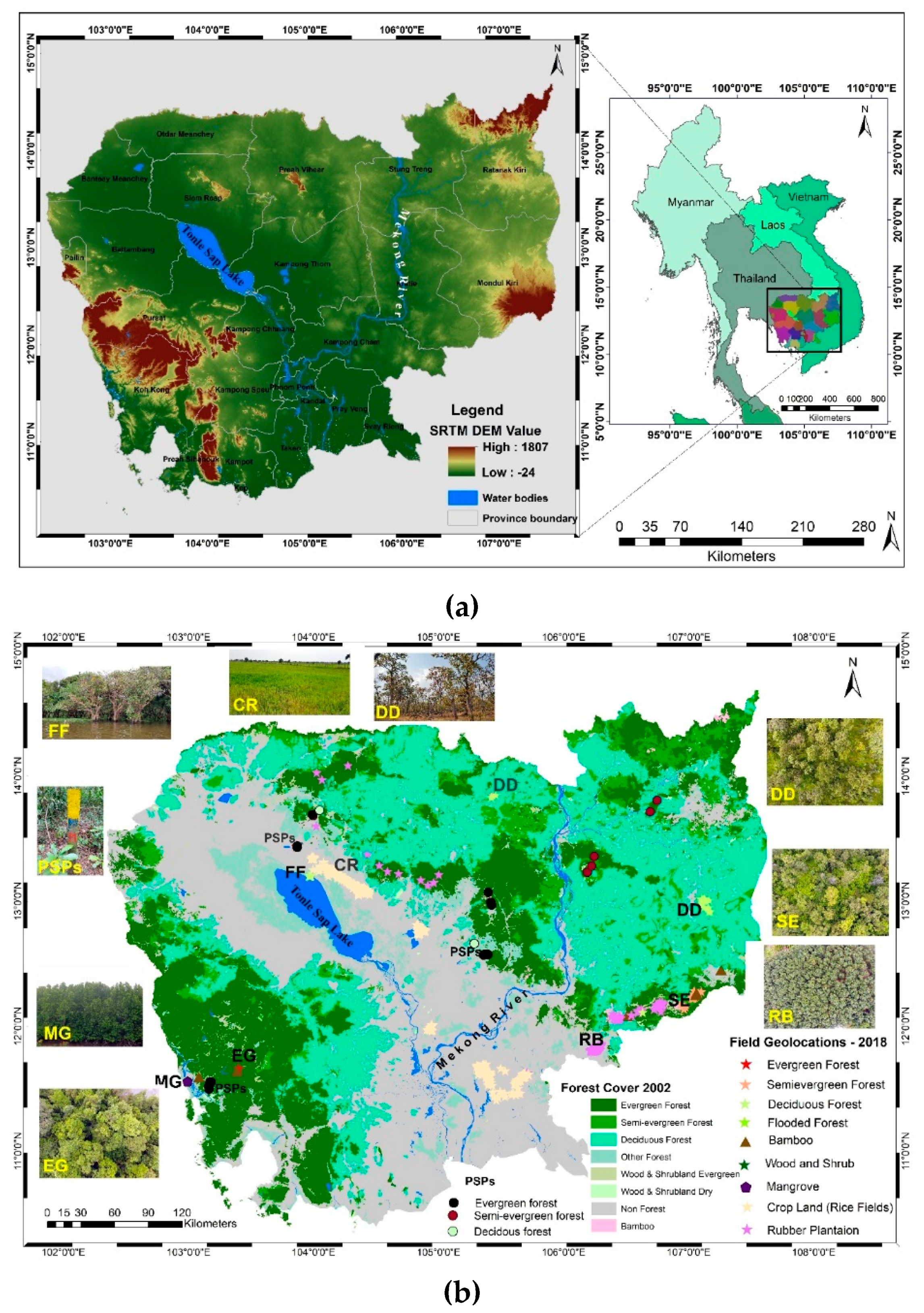
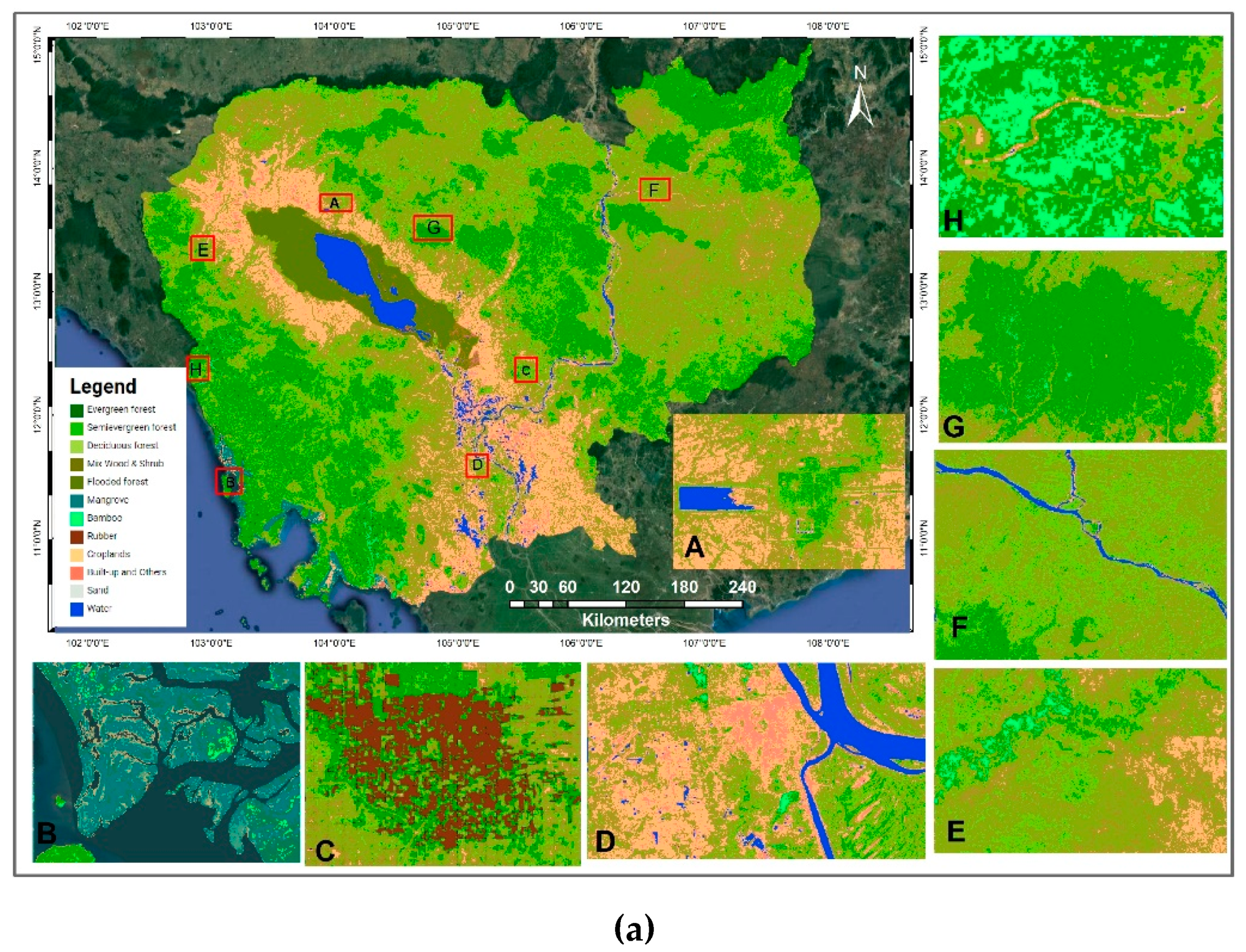
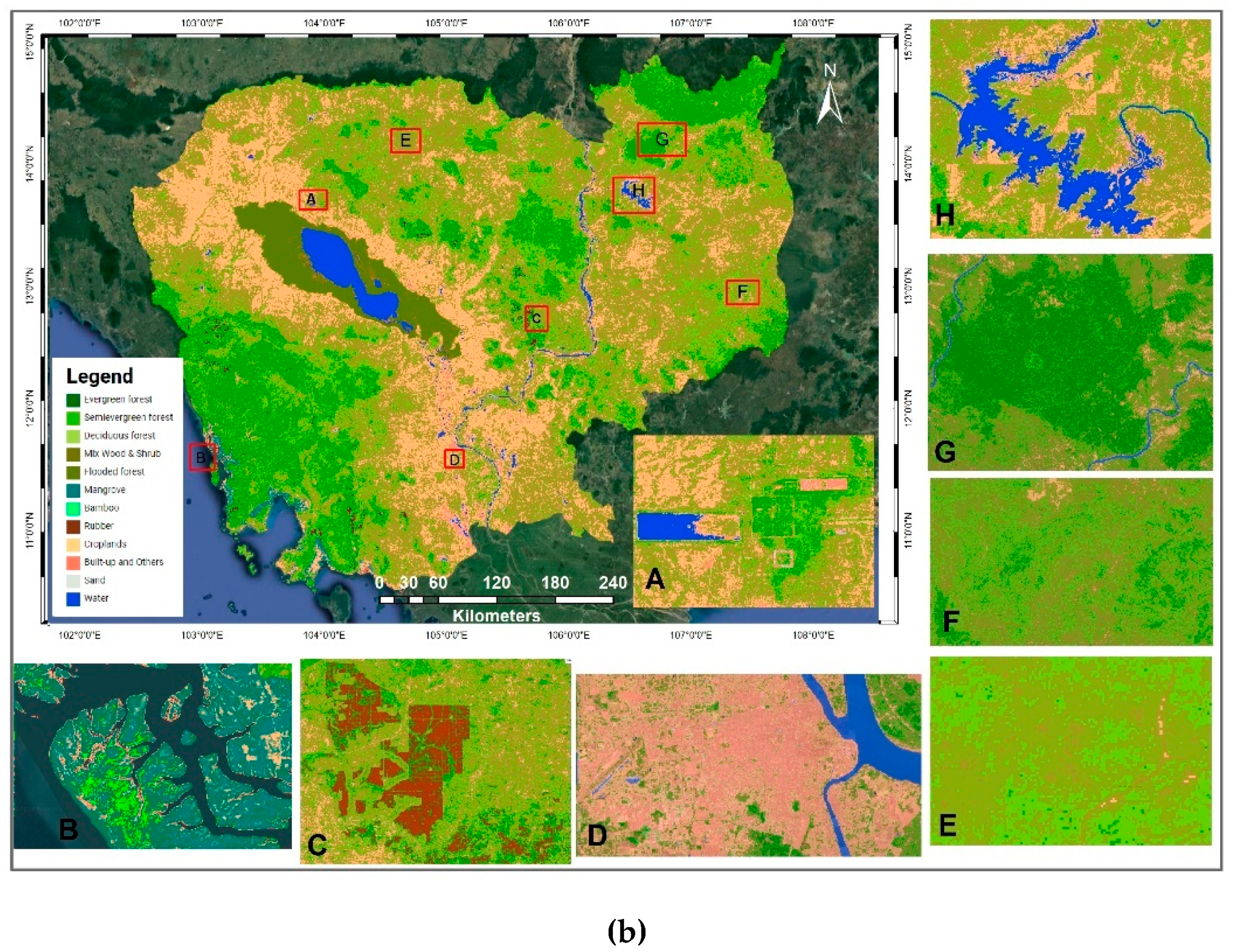
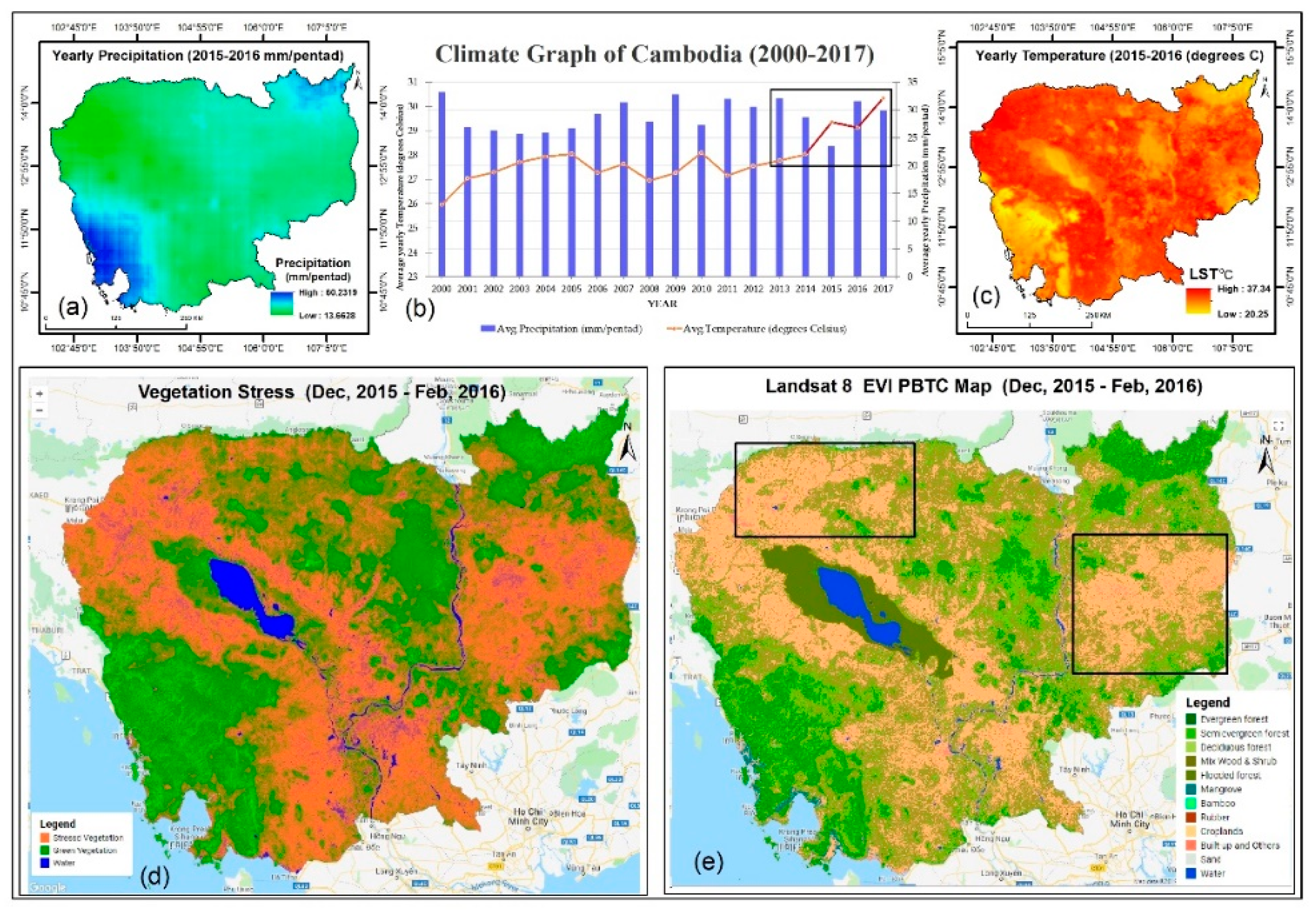
2.1. Study Area

The study area is shown in Figure 1a, and ground reference data are shown in Figure 1b [65]. Cambodia is located between latitudes 10° and 15° North and longitudes 102° and 108° East.

There are four environmental regions in Cambodia: The plain, Tonle Sap, coastal, and plateau and mountainous areas [68]. Cambodia has a tropical monsoon climate and there are two distinct seasons: The dry season from November–April and the rainy season from May–October [69]. The Northwest monsoons (wet) bring 90% of the rainfall, which generally varies between 1200 and 2000 mm per year across the country. The Northeast monsoons result in dry weather in the period of November to April, and the relative humidity ranges from 65–70% in January and February to 85–90% in August and September [68].

There are four major forest types in Cambodia: Evergreen, semi-evergreen, deciduous, and other forests [2]. More than 80% of the plant species in the evergreen forests are evergreen, maintaining their green leaves throughout the year. The semievergreen forest category incorporates a variable percentage of evergreen and deciduous trees. In deciduous forests, more than 80% of the plant species are deciduous species that shed their leaves during the dry season which spans from November–April. The other forest categories include forest re-growth, inundated forest re-growth, inundated forests, mangrove forests, forest plantations, and inundated mosaic forests [65], but this forest type only represents a small proportion of the total forest cover in Cambodia.

Cambodia’s major crop is rice. Rice is classified into four categories: Upland, rain-fed lowland, deep water, and irrigated rice. The Tonle Sap and lower Mekong zones have rain-fed, deep water, and irrigated ecosystems. In rain-fed lowland, rice fields are distinguished by their topography as upper-, middle-, and lower-based [70]. The majority of country agriculture production is dependent on rainfed lowland rice for which the rice sowing season starts in late April or May, the growing period is from September–November, and the harvesting time is between December and February. Likewise, for dry season crops (including irrigated rice) sowing starts in November, the growing time is from January to February, and the harvesting time is between March and April. The planted irrigated rice (dry season crops) can be noticed around Tonle Sap and lower Mekong areas [71]. Other crops, such as maize, soya, which are mostly grown during the dry season, cassava, cashew, rubber, and oil palm, can be seen in the upper to middle topography areas in the study region [72].

Although Cambodia classifies land cover categories into many different classes such as forest, croplands, shrubs, grasslands, and bare areas, it adopts the national land cover categories based on the Intergovernmental Panel on Climate Change (IPCC) guidelines as per the decisions of the UNFCCC at the COP21 [73]. Taking these new land cover categories into consideration, we selected 12 major land cover categories (

Table 1. The 12 land cover categories those vegetation thresholds are to be determined in this study.

No.	Land Cover Categories Used in This Study	Acronyms/ID	Description
1	Evergreen forest	EG	Forests where more than 80% of tree species maintain their leaves throughout the year.
2	Semievergreen forest	SEG	Forests containing a mixture of evergreen and deciduous tree species.
3	Deciduous forest	DD	Forests where more than 80% of tree species are deciduous, shedding their leaves during the dry season of the year.
4	Mix wood and shrub	MixWS	This category consists of a mixture of evergreen and deciduous short tree species and is predominantly covered by shrubs or crops
5	Flooded forest	FF	These forests are permanently underwater, except in the dry season. They are mainly distributed in Tonle Sap Lake and along the riverbanks.
6	Mangrove forest	MG	These forests are located along the coastal areas of Cambodia, where mangrove species are dominant.
7	Bamboo	BB	This is a land category dominated by bamboo
8	Rubber plantation	RB	This category refers to rubber plantations
9	Croplands	CR	This category includes arable land, tillage land, and paddy fields
10	Built-up area	BL	This category includes building and construction areas
11	Sand	SN	This category includes sandy land
12	Water	WA	Areas with fresh and sea water

), those vegetation thresholds were determined in this study. These 12 categories are sufficient to represent all ecosystem types in Cambodia.

2.2. Collection of Landsat Data and Image Composite

Temporal land cover change monitoring is needed to assess the anthropogenic impacts of climate change on the Earth’s ecosystem and to propose appropriate interventions for natural resource management [74,75]. The Landsat satellite acquires over 40 years of data every 16 days. These data have been used for several phenological application purposes in forestry [76,77], cropland mapping [64,78,79,80], land cover classification [53,54], and carbon accounting [56]. Many land surface phenology studies have found that Landsat images can be used with high accuracy [25,28,37,50,51,56,64,81,82,83].

Using the freely available Landsat datasets in GEE, we selected existing Landsat 5 TM (from January 2000–December 2001) and Landsat ETM 7 TOA ortho-rectified collections (from 1 January 2002–December 2003) and Landsat 8 OLI TOA ortho-rectified collections from 1 January 2014–December 2017, covering the whole area of Cambodia. Since Landsat 5 data between January and September are not available in GEE for 2002 and 2003, we merged the Landsat 5 and Landsat 7 datasets in GEE for the phenological assessment (hereafter, ETM and TM are called TM). Here we selected Landsat TM/ETM+ imagery between 2000–2004 because of the availability of the forest reference data from 2000 (Sasaki et al., 2016) for validating study results of Landsat products and geolocating the land cover categories.

We accessed 2199 Landsat images and used these to extract the phenological behaviors of 12 land cover categories. We selected the Landsat 5 TM TOA collections and OLI TOA collections for single EVI threshold mapping. Accordingly, we obtained 159 collections between December to February.

Table A1. Image dates and number of Landsat collections accessed from the GEE for land surface phenology extraction in this study.

		L 5 TM TOA		L 7 ETM TOA		L 8 OIL TOA
PATH	RAW	2000	2001	2002	2003	2014	2015	2016	2017
124	50	15	15	11	13	19	21	21	17
	51	10	13	10	14	19	21	19	18
	52	14	11	9	15	22	20	19	21
125	50	12	9	15	12	17	20	19	15
	51	11	10	13	12	14	16	13	12
	52	14	12	13	12	19	21	18	18
	53	16	12	12	14	19	17	19	18
126	50	14	9	14	15	17	16	16	15
	51	14	10	16	12	21	20	18	16
	52	20	11	14	13	23	20	20	18
	53	16	10	12	13	21	19	19	18
127	50	16	10	11	13	20	20	19	18
	51	14	10	9	11	17	22	22	20
	52	17	10	10	12	17	21	21	17
	53	13	10	10	13	16	18	20	18
128	50	19	12	10	12	19	19	20	17
	51	18	12	11	10	20	20	18	19
	52	3	2	6	6	13	19	11	17
Total Collections		256	188	206	222	333	350	332	312
Observations (%)		11.64%	8.55%	9.37%	10.10%	15.14%	15.92%	15.10%	14.19%

(presented in Appendix A) details the open access Landsat datasets in GEE, which we used for assessing phenology and threshold mapping.

Landsat TOA reflectance-based EVI values were generally higher than surface reflectance (SR) based values [78] and therefore TOA data showed greater potential to provide accurate phenology-based classification [53,79,84,85]. Several studies have successfully applied TOA data for mapping the paddy rice [63,78,79,86,87] and mapping the vegetation distribution [17,22,53,84,88] using phenology-based methods. These studies have suggested that TOA data can be used for mapping with higher accuracy. In this study, we used TOA data to estimate phenological behaviors of the respective land cover categories and to determine the threshold values for better classification of land cover categories in the tropical regions.

Google Earth Engine provides a variety of Landsat specific processing approaches. Specifically, methods to compute at-sensor radiance, TOA reflectance, cloud scores, and cloud-free composites are openly accessible from the GEE [20]. The calibration coefficients of the TOA reflectance orthorectified datasets were extracted from the corresponding image metadata [89]. The GEE has already converted digital number (DN) values into TOA data by putting all remote sensing data from different sensors onto a common radiometric scale, thereby minimizing spectral differences caused by acquisition time, Sun elevation, and the Sun-Earth distance. Methods of converting data into TOA reflectance data are described in Reference [89]. In this study, we used Landsat TOA EVI data to estimate the phenology of selected land cover categories and land cover classifications.

We applied GEE algorithms to composite Landsat imagery and reduced the imagery to median pixel values [5]. The image composition defines the target reflectance of the composited TOA image. The median provides the finest balance between oversaturated and lower pixel values. Lower values focus on low vegetation greenness in the dry season composites and avoid oversaturated pixels. Upper values focus on high vegetation greenness and growing season composites; however, these values can include artifacts due to clouds and oversaturated pixels [5,89]. We observed that 60–75% of the study region was covered by cloud from May–November and 30–40% had cloud cover from December–April. The northeastern mountains, northern plains, Mekong alluvial plains, and coastal range have 35–45% cloud over for almost the entire year. To minimalize the cloud problem, we applied the GEE cloud thrash/mask function algorithm to the entire Landsat collection for the purpose of identifying the imagery with less than 40% cloud cover and for avoiding the bad collections. After that, we applied cloud masking function over the images in order to extract the EVI time series profiles of the selected land use categories between 2000–2003 and 2014–2017.

To determine the surface phenology of the land cover categories, we selected Landsat EVI time series data for this study, as previous studies stated that the EVI overcomes the saturation problems of the NDVI, especially in areas with dense vegetation [81]. The formula was used to calculate the EVI for Landsat TOA composite image collections with GEE JavaScript:

EVI= G × ((NIR − RED) / (NIR + C1 × RED − C2 × BLUE + L))

(1)

where the coefficients of the EVI equation are L = 1 (canopy background adjustment factor); C1 = 6 and C2 = 7.5 (aerosol correction factors); and G = 2.5 (gain factor) [23,27,63,90]. NIR represents the near-infrared band (TM band 4 and OLI band 5); RED represents TM band 3 and OLI band 4; BLUE represents TM band 1 and OLI band 2 [85,87].

2.3. Reference Data

Ground reference data on land cover categories were randomly collected through field visits in February and July 2018 (Figure 1b). We geolocated 300 sampling points to ensure the exact locations of each land cover category in different locations in the study region. The locations were as follows: EG (12 locations including two Permanent Sample Plots (PSPs), SEG (11 locations including one PSP), DD (40 locations including 1 PSP), FF (9 locations), paddy fields (120 locations), rubber (90 locations), bamboo (10 locations), and MG (8 locations). A field survey was conducted, which focused on the placement of PSPs and covered the main land cover categories in five provinces, namely Siem Reap, Mondulkiri, Takeo, Koh Kong, and Preah Vihear (Figure 1b). All the field-based geolocations were recorded using WSMaps mobile app (http://swmaps.softwel.com.np/). We flew the DJI Phantom 4 pro drone at five locations: SEG forests in Koh Kong and Mondalkiri provinces, DD forests in Mondulkiri and Takeo provinces, and an RB plantation in Mondulkiri province (Figure 1b). The drone aerial photos were processed using the Pix4D (https://www.pix4d.com/) drone image processing tool for mosaicking the photos and ortho-rectifying the drone images. The orthorectified image geometric corrections were automatically done in Pix4D. The orthorectified images were imported into GEE using the assets manager, and the drone image geolocations were verified by overlaying them on the GEE VHR image before assigning the geometry. After validation of the drone images, we determined the geometry of the forest types.

Prior to utilizing the ground reference data, we improved the reliability of the reference dataset by cross-validating forest cover data from 2002 and 2006 at the commune level (Figure 1b). A detailed land cover mapping method used in 2002 and 2006 was reported in Reference [65]. We used these data to validate the geometric locations of forest categories in GEE, namely EG, SEG, DD, BB, and Mix WS. These data were also used to assess the accuracy of the resulting threshold spatial maps.

In addition to improving the ground reference data, we collected the locations of PSPs. The forestry administration established the PSP system in 1998 with five or eight clusters with four main plots (each plot 50 × 50 m) and four sub-plots (each 20 × 20 m) for each of the five provinces in Cambodia (32 plots for Kratie and 20 plots each for Karatie, Siem Reap, Kokong, and Ratanakiri) [91]. For this study, we selected 4 PSPs in Siem Reap province followed by EG, SEG, and DD; 3 EG PSPs in Kokong province; and 6 PSPs (5 EG and 1 DD location) in Kampong Thom province. In addition, we geolocated 5 SEG forest inventory locations in Kratie and Ratanakiri provinces by referring to Figure 1b [67]. The forest cover types (2002 and 2006), PSPs, and SEG sampling locations were cross-validated using field reference data and high spatial resolution Google Earth images to produce the reference data for this study.

We imported the reference data (ESRI shapefile) into GEE using the GEE Assets Manager tool and determined the geometry of the reference data using the GEE geometry tool to get the EVI phenology of the individual land cover categories (Figure 2). Eventually, we validated the EVI profiles and selected 10 geometries per land cover category, which resulted in 120 geometries for 12 land cover categories, which were used for the GEE phenological assessment of the selected land cover categories.

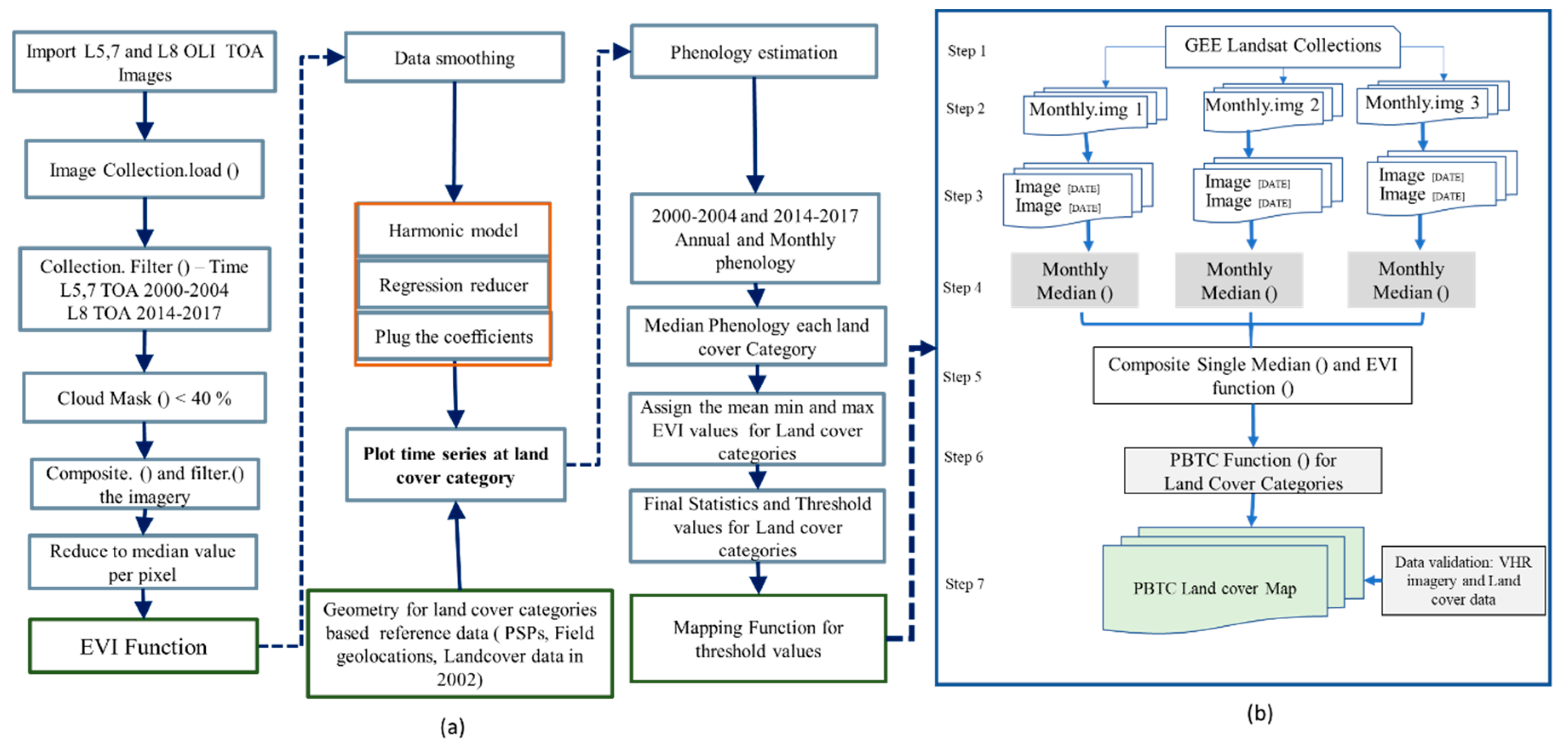
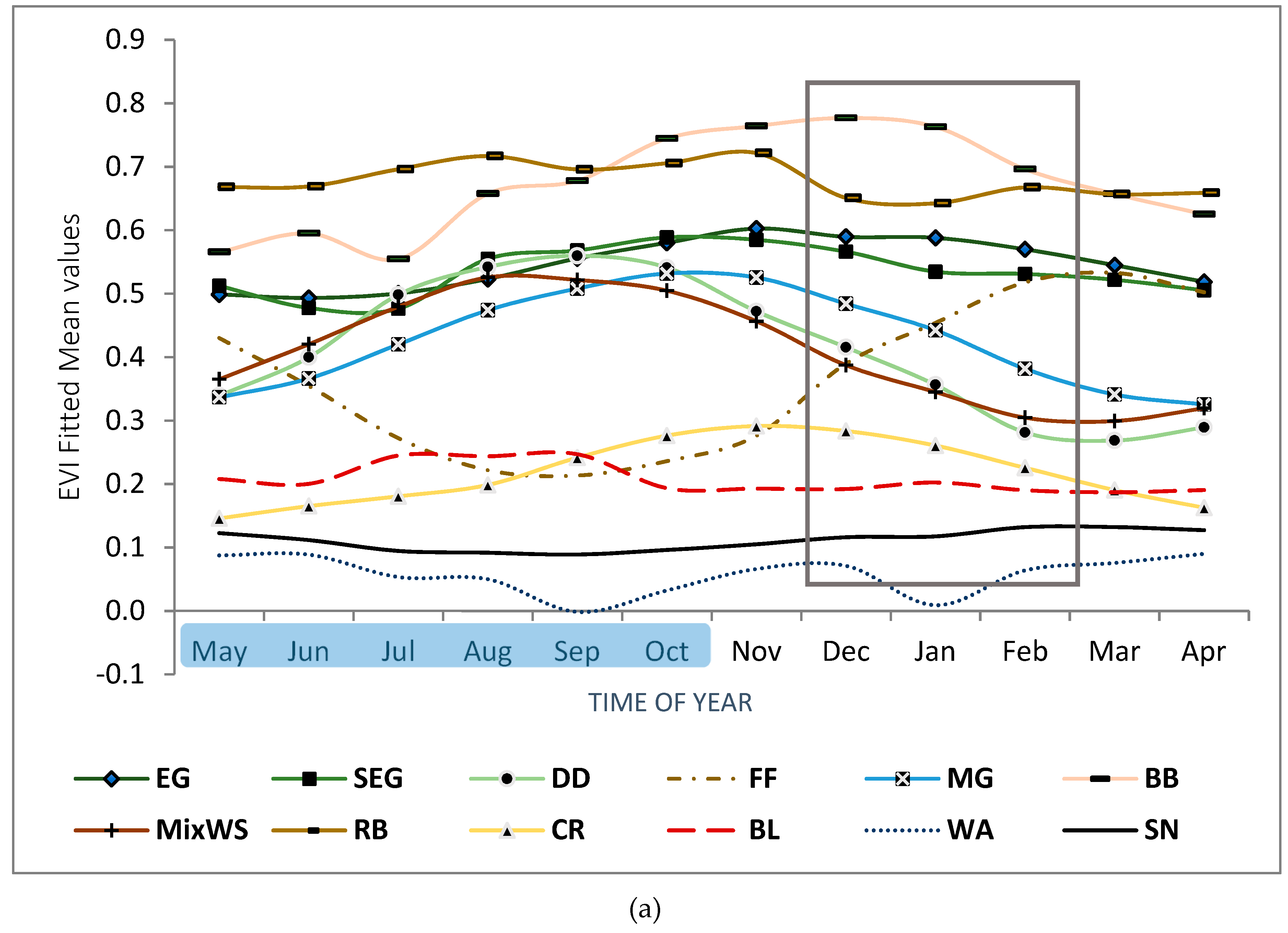
2.4. Land Surface Phenology Approach

Specifying the land surface phenology is essential and useful for detailed mapping, and it avoids the frequent misclassification of land cover types. However, having spectral knowledge of the land cover categories is preferable because spectral reflectance values vary over land cover features and time. Therefore, it is advantages to harmonize time-series remote sensing data with the phenological cycle. We used the fast computing abilities of GEE to extract the temporal time series of spectral characteristics of the land cover categories from the GEE harmonic regression model of the TM and OLI collections.

Harmonic regression is a mathematical technique that is used to decompose a complex, static signal into a series of individual sine or cosine waves, each characterized by a specific phase and amplitude [92]. The harmonic fitting method procedure of the GEE was presented by Nick Clinton (GEE relations developer) during the GEE 2016 User’s Summit (details on the time series harmonic model algorithms can be found at https://developers.google.com/earth-engine/tutorials#time-series-analysis). We adapted Nick Clinton’s GEE harmonic regression algorithms for Landsat collections to estimate EVI fitted and original time series values for selected land cover categories. A detailed flowchart of phenology estimations and the threshold mapping approach is shown in Figure 3, and the following steps were carried out to assess the phenological behaviors of major land cover categories in this study:

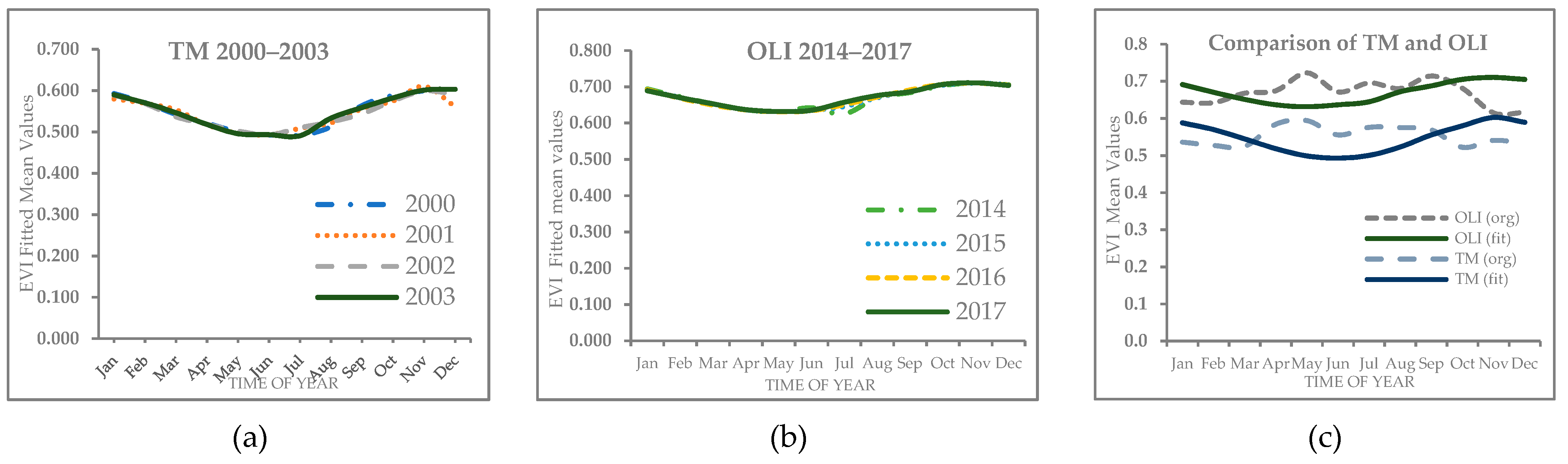
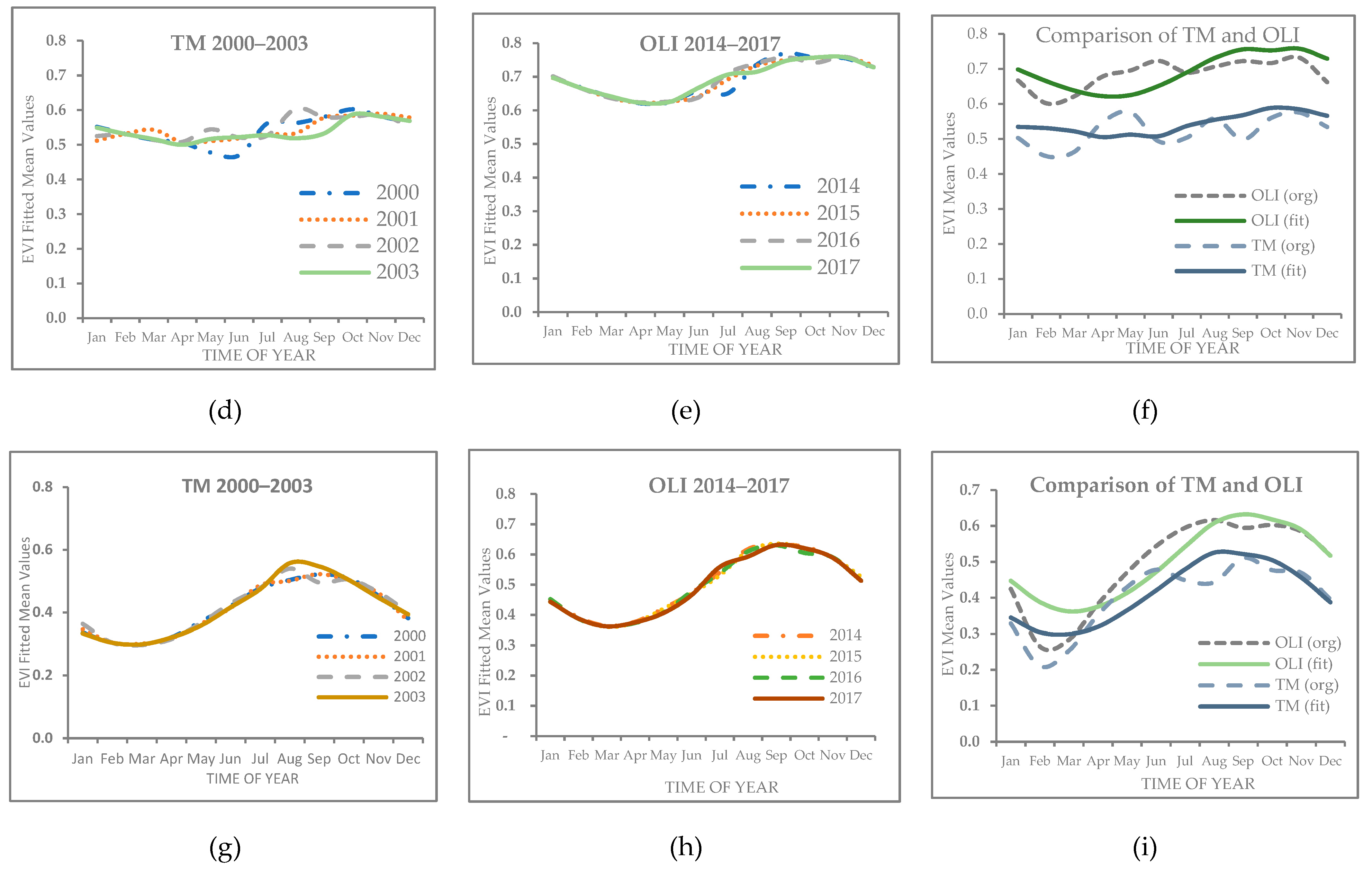
• Landsat TM TOA and Landsat OLI TOA data were collected from the GEE. The underwent preprocessing and the time series of the collections were filtered. The image filter function and the composite, and reducer functions were applied to determine the median values within the study region. The EVI function was used to determine the phases of the composite median imagery.
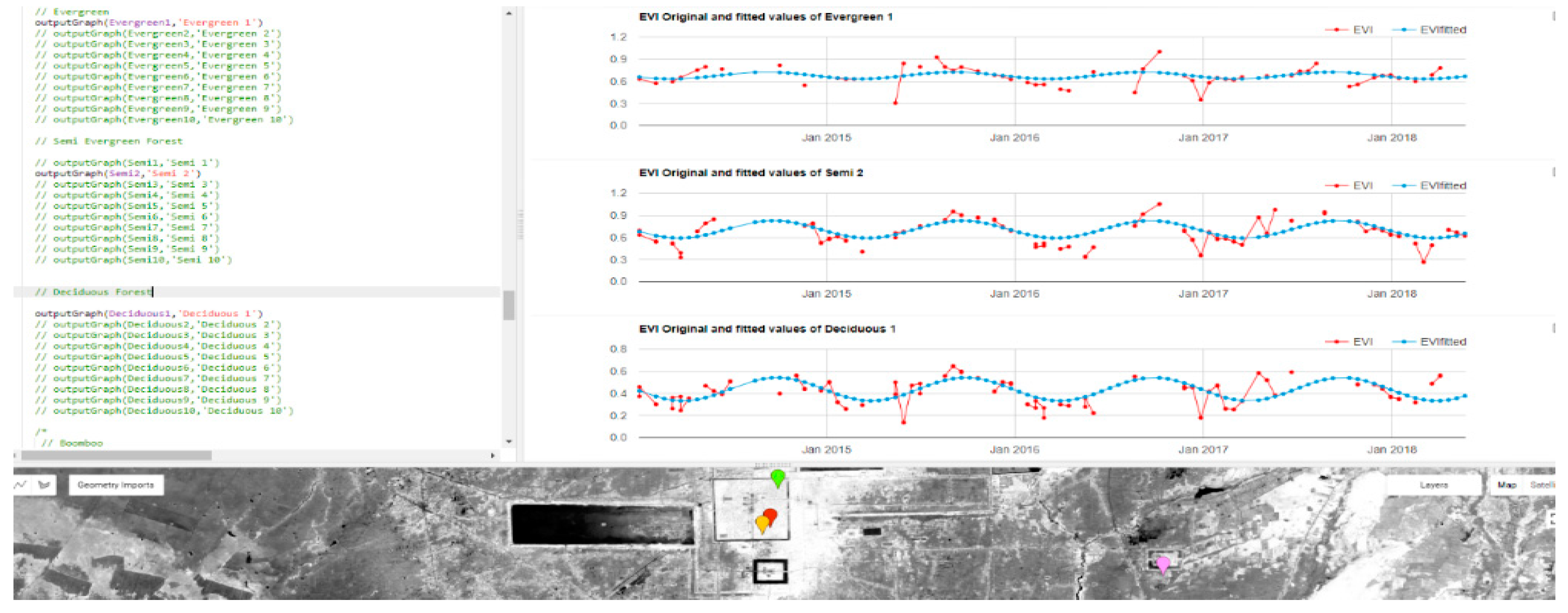
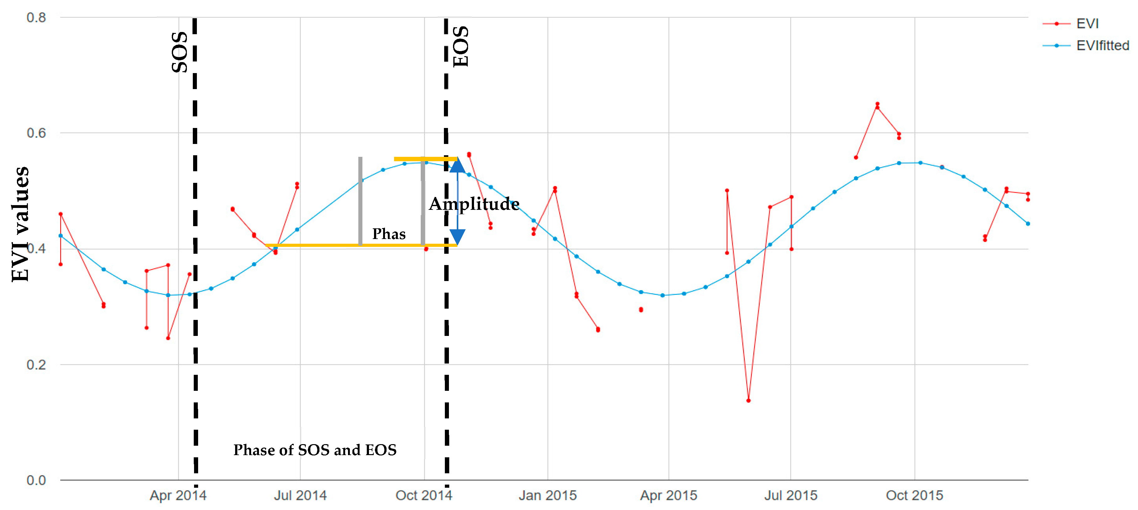
• The data were smoothed and the geometry was plotted on reference land cover data to form temporal EVI profiles. The harmonic model function was used to compute the linear regression reducer, and the coefficients were plugged into the linear model to get the phase and amplitude.
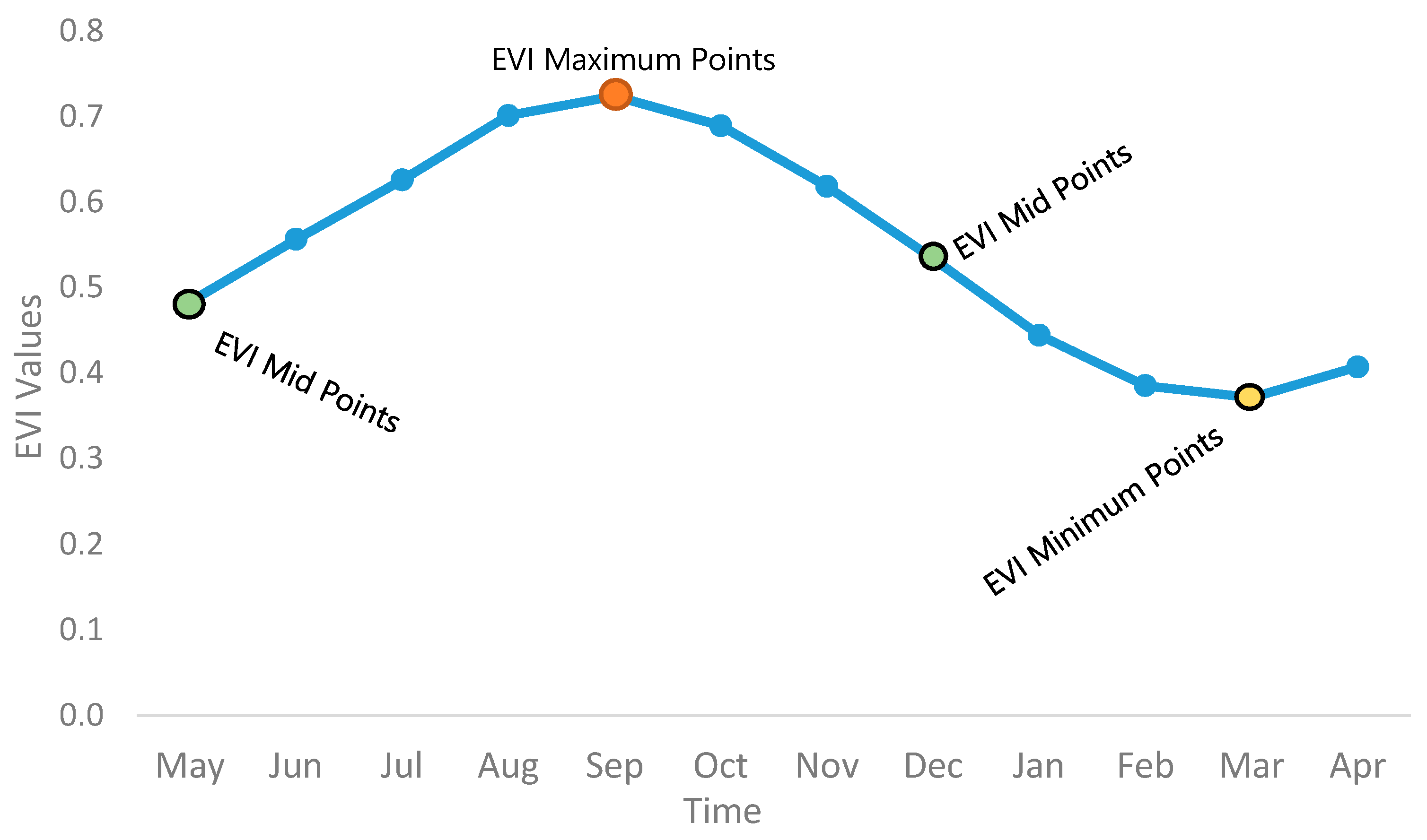
• For phenology estimation, the average and mean EVI profiles of pixels of corresponding land cover types were calculated, and a search process was used to determine the phenology parameters, e.g., high-peak values and low values in time were identified through LSP and LFP as well as SOS and EOS. The threshold values for individual land cover categories were determined at specific phenology phases.
• To develop the mapping function for single EVI data, the GEE image reducer and median function were used to form composite time series images to give a single median EVI. The PBTC function was applied for median EVI classification. Eventually, the resulting threshold maps were validated using a VHR Geographic Information System (ArcGIS) image and reference forest cover data.

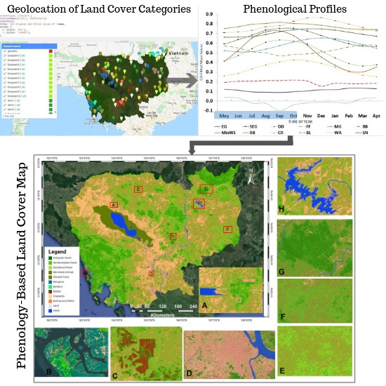
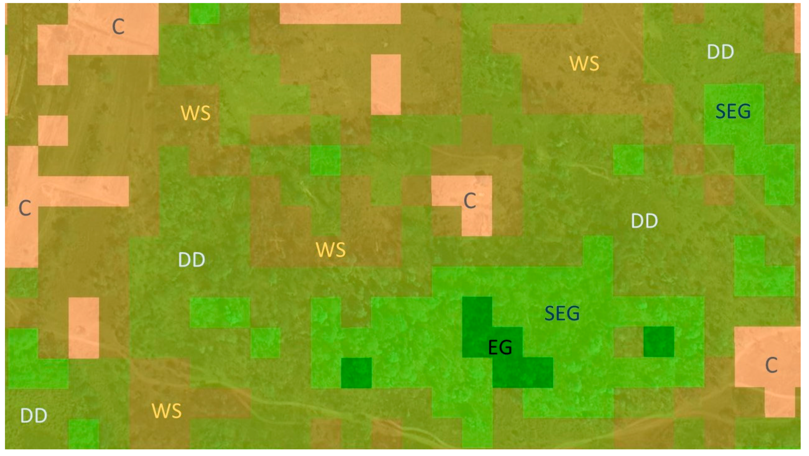
2.5. Selection of Land Cover Categories for the Phenology Assessment

To examine the phenological characteristics of the land cover categories, we selected major 12 land cover categories: EG, SEG, DD, FF, MG, MixWS, BB, CR, RB, BL, SN and WA. Due to a lack of reference data and spatial resolution, pine plantations, tree plantations, forest regrowth, and oil palms were merged, where their spectral reflectance was similar to the EG, SEG, DD, and Mix WS categories. The grassland category was merged with the cropland categories as its spectral behaviors are similar to those of croplands during the selected phenological seasons, and the spatial distribution of grass in the study region is minor.

We identified 240 geometries for the 12 land cover categories and 10 geometries for each land cover type (Figure 4) by referring to the reference data (Figure 1a,b) from the TM and OLI collections. BL, SN and WA geometries were marked based on image visual interpretation in GEE.

Google Earth Engine generated fitted and actual EVI profiles were stored in comma-separated value (CSV) files, which we exported outside of GEE and Microsoft Excel was used for further statistical analysis. Based on the spatial resolution and the value of each Landsat pixel (30 m), the harmonic-fitted mean EVI and the original mean EVI values were calculated annually and monthly (

Table 2. A number of harmonic EVI profiles were produced to estimate phenology and determine the threshold values for selected land cover categories.

Land Cover Categories	Original Mean EVI Profiles of TM/ETM+ and OLI		Fitted Mean EVI Profiles of TM/ETM+ and OLI		Average Yearly Original EVI Profiles		Average Yearly Fitted EVI Profiles	Fitted Mean Profiles (SOS–EOS)			Fitted Mean Profiles (LFP–LSP)	Final Mean LSP Profiles
	2000–2003	2014–2017	2000–2003	2014–2017	TM/ETM+	OLI	TM/ETM+	OLI	TM/ETM+	OLI	TM/ETM+	OLI	TM/ETM+	OLI
EG	10	10	10	10	4	4	4	4	1	1	1	1	1	1
SEG	10	10	10	10	4	4	4	4	1	1	1	1
DD	10	10	10	10	4	4	4	4	1	1	1	1
WS	10	10	10	10	4	4	4	4	1	1	1	1
FF	10	10	10	10	4	4	4	4	1	1	1	1
MGR	10	10	10	10	4	4	4	4	1	1	1	1
BMB	10	10	10	10	4	4	4	4	1	1	1	1
RBR	10	10	10	10	4	4	4	4	1	1	1	1
CR	10	10	10	10	4	4	4	4	1	1	1	1
BL	10	10	10	10	4	4	4	4	1	1	1	1
SN	10	10	10	10	4	4	4	4	1	1	1	1
WA	10	10	10	10	4	4	4	4	1	1	1	1
Total	120	120	120	120	48	48	48	48	12	12	12	12	1	1

and Figure 5).

This resulted in the formation of 722 mean EVI profiles for 12 land cover categories, which described the behaviors of the land cover categories vegetation index spectral response at the SOS and EOS as well as during LSP and LFP.

We observed missing original EVI pixel values at some geometry locations of land cover categories on both TM and OLI images between June and September. The missing data could be due to clouds on the imagery. We compared both original and fitted EVI values and found that the fitted mean EVI values had higher accuracy than the original EVI values (Figure 5c,f,i). Therefore, we used the harmonic-fitted EVI values for phenology estimation in this study.

2.6. Land Cover Category Phenology and Validation

Previous studies have applied numerous methods to extract land surface phenology metrics from time series of remote sensing images by adopting two definitions for SOS and EOS [45,93]. These are based on the mid-values at the start of the season in the time series and the peak values of the second derivative of the growing season curve [94]. Some studies have suggested that the peak-values agree more closely with the phenological transitions observed on the ground [93] because of the biophysical meaning of this definition [95], and other studies stated that the mid-values are a more reliable method for determining vegetation phenology because of uncertainty (due to snow cover and cloud contamination) of the remote sensing time series images [96].

Here, we observed the seasonal variation in the vegetation indices as a general trend in the EVI time series, where high values were accrued towards the end of the growing season (August–October) and low EVI values were accrued during the dry season (February–April). We identified the seasonal minimum and maximum EVI values using the annual fitted harmonic profiles of each land cover category as indicators of the LSP and following LFP (Figure 6). We also identified the peak-value phase between SOS and the decaying end of the phenology season (EOS) [27] (Figure 7).

For determination of the EVI phenological mid-values [96], the ratios of the EVI amplitude to the annual mid-value in the early growing season (May–July) and early dry season (December–February) were calculated to determine minimum and peak-values of each land cover category during the mid-phenology vegetation index phase. We observed uncertainties (cloud and shadow) in the Landsat time series images during the growing season (local rainy season) and overlapping profiles of vegetation indices (EG, SEG, DD, BB, MG, and RB). Further, we validated all mean vegetation index values of each category and found a separation gap in the EVI mean profiles during the dry mid-LSP season (December–February).

Subsequently, the mean EVI profiles of the 12 land cover categories during the dry mid-phenology season were identified by separation gaps in the mid-LSP season; however, the spectral characteristics of the FF and MG species were similar to those of other forest categories during the mid-LSP season. To avoid misclassifying FF and MG, we created a boundary for the Tonle Sap flooded forest and the mangrove forest using the GEE geometry tool through visual interpretation, and we separately assigned threshold values to classify them. To determine the threshold values for individual land cover categories, we validated the mid-LSP season EVI mean standard bar values and selected standard bar low values that did not overlap with other categories as minimum threshold values. The mid-LPS season high-peak values were assigned as maximum threshold values.

2.7. Phenology-Based Threshold Classification Approach

The GEE cloud computing and image parallel processing capacity make it efficient to run spatial reductions of the image collection. The tile-by-tile processing method of GEE applies a median reducer to each tile of the remote sensing data at a specific season or at a particular time [19].

Here, we applied the GEE image reducer and median function [19,26] to the TM and OLI collections for the dry mid-phenology season (December–February) to get a median EVI for threshold mapping. This involved eight steps. The diagram in Figure 3b illustrates the detailed approach for the single image pixel-based threshold mapping of individual land cover categories: (1) The Landsat collections were accessed using the image collection function in GEE; (2) the reducer function was used to select the seasonal imagery; (3) the tile-by-tile images were converted to the median; (4) the composite function was used to form a median single image for the dry mid-phenology season; (5) the EVI function for the median image was determined; (6) the threshold values for individual land cover categories were assigned; and (7) the PBTC function was used for spatial mapping in GEE.

The GEE basically uses two main programming languages, JavaScript and Python, to compute and analyze the remote sensing imagery. Here, we applied JavaScript to build PBTC algorithms to classify the median EVI data from the single composite Landsat image using predefined knowledge-based fuzzy rules in the GEE. We applied a similar study method developed by Simonetti et al. (2015), this approach which was later implemented in GEE [54].

2.8. Accuracy Assessment

The number of reference points collected during the field survey did not cover the entire study region; therefore, the mapping accuracy of the resulting spatial maps was evaluated using VHR imagery and reference forest cover data. Most commonly, stratified random sampling and systematic sampling are implemented to design reference data for validating classification maps. However, stratified random sampling is a practical design that satisfies the basic accuracy assessment objectives of the remote sensing community [97]. Remote sensing time series data with VHR images can be used to determine the accuracy of reference change data, and the process of generating the reference data is more accurate when the established protocol is followed [97].

To assess the accuracy, a total of 1420 spatial points were established for the study region using the stratified random sampling approach [97]. We used the ArcGIS environment to generate random spatial points by creating 355 reference points for each map from 2000 (TM) and 2018 (OLI). Further, to validate our results, we created 355 random points for each forest cover data reference point in 2000 and 2006, and these data were used for a spatial assessment. Here, the sampling size of the reference data (355 sampling points) was used for assessment of the resulted maps. This was to ensure that each land cover category was properly represented by referenced points, thereby reducing bias in the accuracy assessments. We converted the accuracy points to polygons using ArcGIS Future Envelope to Polygon tool to evaluate the classified maps with 30 m pixels. The TM map (2000) reference points and polygons were converted to KML format and exported into Google Earth for validation using Google Earth timescale temporal imagery from 2000. The OLI 2018 map was validated with ArcGIS using VHR imagery.

The reference forest cover maps were classified into 8 categories (Figure 1b): EG, SEG, DD, other forests (OF), wood and shrub evergreen (WE), wood and shrub dry (WD), non-forest (NF), and Bamboo BB. To evaluate the reference forest cover map accuracy, we merged the threshold map categories: CR, BL, SN, and WA were merged into the NF category; FF, MG, and RB were merged into the OF category; and WE and WD were merged into the MixWS categories. The major forest categories, EG, SEG, DD, and BB, were kept the same. The resulting PBTC maps were exported to Google drive using the export function in GEE. We extracted the resulted phenology-based threshold map category labels from the spatial accuracy points using the ArcGIS spatial analysis tool. The reference forest cover maps from 2002 and 2006 and the threshold maps were overlapped in ArcGIS, and they were visually interpreted with the accuracy points.

We analyzed a 30 m Landsat pixel window using accuracy polygon and accuracy sampling points data in ArcGIS and Google Earth, which permitted us to interpret the resulting phenology-based threshold maps to determine the minimum and maximum tree and crown cover in single Landsat pixels (Figure 8).

The accuracy points were compared to the corresponding classified pixels in VHR images in ArcGIS and Google Earth and with existing land cover maps. The percentage of agreements was recorded in an accuracy table. Eventually, the assessment datasets were used to assess the classification accuracy using a confusion matrix [97]. We calculated the overall accuracy, the producer’s (errors of omission) accuracy, the user’s (errors of commission) accuracy, and the kappa coefficients over the confusion matrix for both classified threshold maps.

3. Results

3.1. Phenological Behaviors of Land Cover Categories from Multi-Temporal Landsat Imagery

Cambodia has a monsoon climate and its spatial phenological behaviors vary greatly depending on the geographical location, land use management, and land cover types. Changes in the phenological behaviors of land cover categories caused by variations in environmental proximate factors may have shaped those behaviors. The results of the EVI profiles of the tropical region land cover categories phenology behaviors are shown in Figure 9a,b.

The obtained mean EVI phenological profiles of the forest and cropland categories show the high-peak vegetation index values accrued at the end of the growing season (rainy season) from August–October and the mid EVI values observed during the growing season (May–July) and dry season (November to January) from 2000–2003 (TM) and from 2014–2017 (OLI) (Figure 9a,b). In the dry season, the EVI values of the forest and croplands category rapidly decreased from December–April, and low EVI values were accrued from March–April. The BL and SN profiles did not change much, and their spectral values stayed at a similar amplitude in both seasons. However, the separation of the gap between most of the selected land cover categories in the mid-dry phenology period between December–February is worth noting (in Figure 9a,b), see the three years mean phenology characteristics window; the box indicates the separation of the vegetation index profiles of the major land cover categories.

Comparing the phenology-based EVI profiles of land cover categories (Figure 9a,b), BB and RB showed greater vegetation index differences than EG and SEG over the entire phenological period from 2000–2003 and from 2014–2017. The BB minimum and maximum peak values (TM: 0.764–0.777; OLI: 0.860–0.863) occurred during the EOS and the start of the dry season (November–December), and the low-values (TM:0.566–0.554; OLI: 0.707–0.716) occurred at the start of the rainy season, from May–July. The RB high vegetation index values (TM: 0.722–0.651; OLI: 0.784–0.798) greater than the BB (TM: 0.554–0.566; OLI: 0.707–0.716) values at the SOS (monsoon/rainy season) from May–August and the RB EVI profiles were slightly down (OLI: 0.741–0.748, TM: 0.659–0.668) right after the start of the mid-dry season (January–April). The RB plantations had more variation in leaf-shedding and leaf-flushing behaviors in both seasons as compared to other forest types, and they maintained their leaves at a maximum level (Figure 9a,b). However, leaf-shedding of RB was noticed in the mid-dry season (December–February) and this overlapped twice with BB in both seasons (March and September).

The SEG (TM:0.549–0.589; OLI: 0.733–0.753) and Mix WS (TM:0.544–0.596; OLI:0.677–0.726) peak EVI phenology values were greater than the EG vegetation index values (TM:0.523–0.580; OLI:0.690–0.738) in the mid-LFS period (middle of SOS) between August and October. The DD (TM:0.541–0.560) EVI values between 2000–2003 showed comparable values to those of EG, while the OLI DD vegetation index values (OLI:0.470–0.512). The spectral reflectance of fully flushed new leaves of DD, EG, and mixed BB species showed greater indices values than the sampling pixels of SEG and Mix WS, particularly at the end of the LFP phase between July and September. The separation of SEG, DD, and Mix WS vegetation index profiles from that of EG can clearly be observed from the start of the LSP period (Figure 9a,b), while some deciduous trees may start flowering or leaf-shedding from September; thus, the DD tree profiles dramatically decreased in EOS.

The phenology profiles of the other forest categories, MG and FF, showed a high level of overlap with DD and Mix WS during the growing season and with SE in the dry season (Figure 9a,b). The MG vegetation index high-peak values (TM: 0.381–0.532; OLI: 0.509–0.654) were accrued in the mid-dry phenology period and the FF high-peak values (TM: 0.213–0.518; OLI: 0.471–0.581) were observed at the end of the dry season. The FF profiles dramatically decreased during the months of July to October (rainy season), and they were mixed with croplands from 2000–2003. This is probably due to the increase in the water level in the Tonle Sap lake during the rainy season and the mixing of the reference pixels of FF and WA. In 2014–2017, a separation of the FF profile from that of CR can be seen clearly. This is probably due to a decrease in the WA level in the lake, resulting from the changes in precipitation patterns in the region in the past ten years.

When determining the phenology profile of croplands (paddy fields) per pixel, we clearly observed high EVI values (TM: 0.276–0.291; OLI: 0.417–0.426) during the growing period (October–November) and a decrease in the vegetation index profile was seen right after the harvesting period in dry-mid LSP (December–February). The BL, SN, and WA widely separated from the vegetation index across all seasons studied. It was observed that in the selected land cover categories, the greatest differences in the vegetation index profile among the forest, rubber, croplands, and non-forest categories were found during the mid-dry LSP season (November to February).

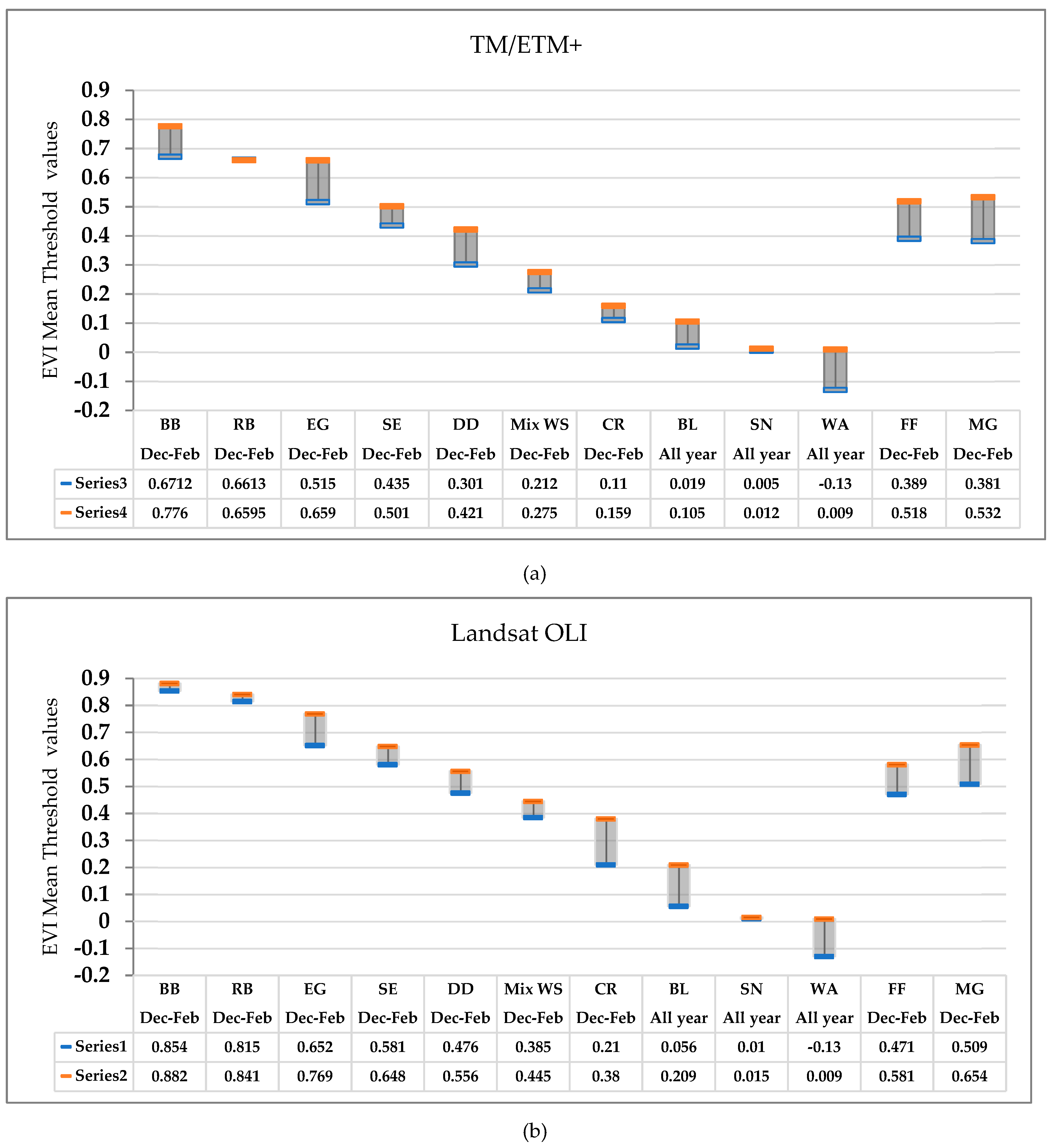
3.2. Mid-Dry Phenology and Threshold Mapping

As shown in Figure 10, the mid-LSP results indicated TM and OLI threshold values and suitable months for classifying the Landsat EVI data for accurate land use and land use change mapping. The threshold values were obtained by validating 722 mean EVI profiles during the leaf-flushing and leaf-shedding seasons.

Bamboo was found to have highest vegetation index values in the mid-dry phenological phase, and the amplitudes of the minimum and maximum threshold values were determined (TM: 0.672 to >0.776; OLI: 0.854 to >0.882) for both TM (Figure 10a) and OLI (Figure 10b) imagery. Similarly, RB showed the highest vegetation index, but the range of the threshold amplitude (TM: 0.659–0.661; OLI: 0.815–0.841) was smaller between BB and EG. The EG (TM: 0.435–0.501; OLI: 0.581–0.648) and DD (TM:0.301–0.421; OLI:0.476–556) forests had greater amplitudes in the determined threshold range in the dry-mid LSP phase as compared with the SEG (TM:0.435–0.501; OLI:0.581–0.648) and Mix WS (TM:0.212–0.275; OLI:0.385–0.445) categories. The threshold values of FF (TM:0.381–0.519; OLI:0.382–0.581) and MG (TM:0.384–0.532; OLI:0.402–0.654), were grouped within their homogeneous species vegetation index values. The CR vegetation index amplitude ranged from 0.11–0.159 and 0.21–0.38 for TM and OLI, respectively, during the harvesting period. The BL threshold (TM: 0.019–0.105; OLI: 0.056–0.209) values were determined by combining settlements and building and construction areas. The SN and WA amplitude ranges were found to be less than 0.012.

The obtained phenology-based threshold values were determined for the 12 land cover categories above in the mid-leaf-shedding phase by selecting their high-peak vegetation index values for threshold-based land use and land use change mapping. These minimum and maximum threshold values were 0.652–0.769 for EG forest, 0.581–0.648 for SEG forest, 0.476–0.556 for DD forest, 0.385–0.445 for Mix WS, 0.382–0.581 for FF, 0.402–0.654 for MG forest, 0.854–0.882 for BB, 0.815–0.841 for RB plantation, 0.21–0.38 for CR, 0.056–0.209 for BL, 0.01–0.015 for SN, and −0.13–0.009 for WA for Landsat OLI EIV data. For the Landsat TM EIV data, the threshold values were 0.515–0.659 for EG forest, 0.435–0.501 for SEG forest, 0.301–0.421 for DD forest, 0.212–0.275 for Mix WS, 0.381–0.519 for FF, 0.384–0.532 for MG forest, 0.671–0.776 for BB, 0.659–0.661 for RB plantation, 0.11–0.159 for CR, 0.019–0.105 for BL, 0.005–0.012 for SN, and −0.13–0.009 for WA. Please see

Table A2. Land cover categories mid-dry phenology season median threshold values of TM (2000–2003) and OLI (2014–2017) images.

	Landsat OLI		TM
Land Cover Categories	Min	Max	Min	Max	Suitable Months
BB	0.854	0.882	0.6712	0.776	Dec-Feb
RB	0.815	0.841	0.6595	0. 6613	Dec-Feb
EG	0.652	0.769	0.515	0.659	Dec-Feb
SE	0.581	0.648	0.435	0.501	Dec-Feb
DD	0.476	0.556	0.301	0.421	Dec-Feb
Mix WS	0.385	0.445	0.212	0.275	Dec-Feb
CR	0.21	0.38	0.11	0.159	Dec-Feb
BL	0.056	0.209	0.019	0.105	All year
SN	0.01	0.015	0.005	0.012	All year
WA	−0.13	0.009	−0.13	0.009	All year
FF	0.382	0.581	0.381	0.519	Dec-Feb
MG	0.402	0.654	0.384	0.532	Dec-Feb

in Appendix A for details on the land cover categories mid-dry phenology season threshold values of TM (2000–2003) and OLI (2014–2017) data. Cloud and shadow threshold values were excluded in this study.

3.3. Phenology-Based Threshold Map and Accuracy Assessment

The phenology-based threshold maps were shown to be highly accurate according to the confusion matrix estimated from the random reference data from 2000 and 2018, which validated VHR imagery and reference forest cover data.

Table 3. Results of the accuracy assessment for the TM 2000 and OLI 2018 classified maps. The values of the 12 land cover categories were derived using the final accuracy matrix of the generalized map. The gray cells indicate agreement of the accuracy matrix.

(a) 2018 Assessment GIS VHR Reference Categories
2018 Classified Categories	EG	SEG	DD	Mix WS	FF	MG	BB	RB	CR	BL	SN	WA	User’s Accuracy
EG	50	2			2	2	1	2					84.7%
SEG	3	31	1	1	2	1		1					77.5%
DD			58	2					1				95.1%
Mix WS		1	2	41	1				1				89.1%
FF					10	1							90.9%
MG					1	20							95.2%
BB	1						25	1					92.6%
RB							2	14					87.5%
CR			1	2					54	1			93.1%
BL									1	4			80.0%
SN											1		100%
WA												10	100%
Producer’s accuracy	92.6%	91.2%	93.5%	89.1%	62.5%	83.3%	89.3%	77.8%	94.7%	80.0%	100%	100%	Overall Accuracy 89.58%
Kappa 0.88 Total reference points 355
(b) 2000 Assessment Google Earth VHR Reference Categories
2000 Classified Categories	EG	SEG	DD	Mix WS	FF	MG	BB	RB	CR	BL	SN	WA	User’s Accuracy
EG	47	2			2	1	2	2					83.9%
SEG	2	46	1		2	1	1	2					83.6%
DD		1	78	1	1				1				95.1%
Mix WS	1	1	3	35					2				83.3%
FF					11	2							84.6%
MG					1	8							88.9%
BB	2	1					29	2					85.3%
RB							2	14					87.5%
CR				2					19				90.5%
BL									1	6			85.7%
SN										1	3		75.0%
WA												16	100%
Producer’s accuracy	90.4%	90.2%	95.1%	92.1%	64.7%	66.7%	85.3%	70.0%	82.6%	85.7%	100%	100%	Overall Accuracy 87.89%
Kappa 0.86 Total reference points 355

a,b and

Table 4. Results of the accuracy assessment for the TM 2000 and OLI 2018 classified maps. The values of the 7 land cover categories were derived using the maps with the reference forest cover data in (a) 2000 and (b) 2006.

(a) 2018 Assessment Forest Cover Reference Categories
2018 Classified Categories	EG	SEG	DD	OF	Mix WS	NF	BB	User’s accuracy
EG	45	1		1	1		1	91.8%
SEG		28	2					93.3%
DD		2	57		2	1		91.9%
OF	8	3	5	46	3	4		66.7%
Mix WS			3		36	3		85.7%
NF			1		3	70		94.6%
BB				1			28	96.6%
Producer’s accuracy	84.9%	82.4%	83.8%	95.8%	80.0%	89.7%	96.6%	Overall Accuracy 87.32%
Kappa 0.85
(b) 2000 Assessment Forest Cover Reference Categories
2000 Classified Categories	EG	SEG	DD	OF	Mix WS	NF	BMB	User’s accuracy
EG	42	9			2			79.2%
SEG	8	39	2		1			78.0%
DD		1	72		2			96.0%
OF	2	4	9	25	3	1	2	54.3%
Mix WS			1		32	2		91.4%
NF	1	1	1		1	61	4	88.4%
BMB						2	25	92.6%
Producer’s accuracy	79.2%	72.2%	84.7%	100.0%	78.0%	92.4%	80.6%	Overall Accuracy 83.38%
Kappa 0.80

a,b provide an overview of the overall accuracies (OA), Kappa coefficients, producer’s accuracies (PA) and user accuracies (UA) of the 2000 and 2018 maps validated by VHR imagery. Table 4a,b provides an overview of the overall accuracies matrix validated by the reference forest cover data.

Validation of the 2018 map with VHR imagery (Table 3a) using the confusion matrixes of EG (PA 92.6% and UA 87.7%), SEG (PA 91.2% and UA 77.5%) and DD (PA 93.5% and UA 95.1.5%) showed high accuracy. Similarly, EG (PA 90.4% and UA 83.9%), SEG (PA 90.2% and UA 83.6%), and DD (PA 95.1% and UA 95.1%) showed greater accuracy in the threshold map in 2000 (Table 3b). The FF, MG, BB, and RB categories were the main sources of confusion in the EG and SEG forests, and MixWS was the source of confusion in the DD forests in both classified years (Table 3a,b). Separate mapping of FF and MG can improve the accuracy of EG and SEG forests. On the other hand, BB (PA 89.3–85.3% and UA 92.6–85.3%) and RB (PA 77.8–70.0% and UA 87.5–87.5%) errors occurred between the two categories, and the Mix WS was confused with CR (PA 94.7–82.6% and UA 93.1–90.5%). Furthermore, the minimum randomly sampled accuracy points occurred for the BL, SN, and WA categories with higher accuracy (100%) in both PA and UA.

The validation of the results with reference forest cover data found that the EG (PA 84.9–79.2% and UA: 91.8–79.2%) and SEG (PA 82.4–72.2% and UA 93.3–78.0%) forest categories had the highest consistency in 2018 and lower consistency in 2000 (Figure 6a,b). In addition, the BB (PA 96.6–80.6% and UA 96.6–92.6%) and NF (PA 89.7–92.4% and UA 94.6–88.4%) categories had higher accuracy in both assessment periods. On the other hand, the OF category yielded PA values of 95.8–66.7% and low UA values of 66.7–54.3% in both years, indicating under-classification. Most of the confusion of OF categories with SEG, DD, Mix WS, and NF could have come from the pixel differences between the 2000 and 2006 reference maps. The spread of Mix WS near the croplands and village was considered OF. This could be the reason for the confusion of the OF category with the major forest categories. Nevertheless, the overall accuracy of DD (PA 83.8–84.7% and UA 91.9–96.0%) improved in both referenced maps.

We found that the overall accuracy in VHR of the threshold maps varied from 89.58% in 2018 to 87.89% in 2000 with Kappa coefficients from 0.88 and 0.86 (Table 3a,b), and the overall accuracy of the referenced forest cover varied from 87.32–83.38% with Kappa coefficients from 0.85–0.83 over the same period (Table 4a,b). Among the accuracy results, the forest reference land cover data had lower accuracy. The TM and OLI products both had high spatial consistency in the mapping of phenology-based threshold maps in the tropical region. OLI gave more accurate results than that of the TM for both phenology estimation and threshold map accuracy. However, OLI imagery has a higher capability for threshold-based classification using phenology information compared with Landsat TM data.

Figure 11a,b show Cambodia’s first mid-dry phenology-based threshold land cover map using the PBTC approach with the aid of the fast cloud-computing GEE tool. The threshold maps were classified into 12 major land cover categories in Cambodia: Evergreen forest, semievergreen forest, deciduous forest, mixed wood and shrub (mixed with evergreen and deciduous trees), bamboo, rubber plantation, flooded forest, mangroves, croplands, built-up land, sand or soil, and water as shown in the spatial map legend.

The resulting PBTC maps were identified as being more heterogeneous, distinguished communities of EG, SEG, DD, and Mix WS over the entire study region. The mid-LSP-based threshold maps comparing the TM and OLI images (Figure 11a,b) indicated that the EG forest pixels were well distributed, covering 21.01% of the study region, and this dramatically decreased to 17.56% in 2018. Similarly, SE forest pixels represented 17.40% of the region in 2000 and decreased to 11.67% in 2018. The DD forest pixels were widely distributed (31.08% of the region in 2000) and showed higher accuracy in mapping in the study region, but their distribution declined to 23.45% in 2018. The distribution of the Mix WS pixels decreased from 25.64% to 18.30%. Bamboo was found over the entire region (0.24% in 2000 and 0.17% in 2018), with larger percentages of BB observed in the Northern parts of Ratana Kiri and Stung Treng provinces and in the Western part of the study region, especially in Koh Kong, Pursat, Battambang, Kampot, and Kampong Speu provinces. The distributions of RB (0.14–0.80%) and cropland (10.03–19.15%) pixels increased dramatically from 2000–2018, and the distribution of BL increased from 1.18–1.55%. Regarding the other forest categories, FF is largely found around the Tonle Sap lake and MG is found in Koh Kong, Preah Sihanouk and Kampot, and Kep provinces. However, their percentages of pixel cover may vary when the other forest categories, pine trees, pine plantation, tree plantation, and forest regrowth are included in the threshold mapping.

4. Discussions and Implications

Our study indicates the viability of assessing phenology behaviors and threshold-based mapping of major land cover categories in the tropical region of Cambodia. To our knowledge, this study is the first to assess the phenological behaviors of major land cover categories and to determine threshold values at a 30 m moderate spatial resolution in the tropical region. The GEE freely available fast cloud-computing environment was used to access multitemporal big remote sensing data and computed the massive multitemporal Landsat collections within a limited time period. This study overcame challenges including the effects of cloud cover and missing Landsat observations by determining climatic threshold values and using GEE cloud-computing algorithms.

Firstly, the spatial and temporal resolution of remote sensing data for phenology assessment needs to be selected carefully. In this study, OLI provided high-frequency imagery of 60.35% on average (2014–2017) and TM had average imagery covered of 39.65% (2000–2003) in both the leaf-flushing and leaf-shedding phenology seasons (Table 2). The harmonic regression fitting process which produced the 16 days composite of the entire Landsat collection was performed to provide considerable smoothing of the EVI time-series profiles for both the TM (Figure 9a) and OLI (Figure 9b) datasets. Accordingly, the high-peak values of the phenology-based vegetation index profiles were deducted in the growing season (rainy season). However, the decline of EG, SEG, and BB in the rainy season from July–August (Figure 9a) in the TM images could be due to the minimal observations and high cloud contamination of TM [62]. A previous study found similar results that vegetation index profiles were drastically reduced to the lowest level during the heavy rainy season [98]. On the other hand, the OLI images had more observations across the entire phenology study and showed a realistic vegetation index frequency in both phenological seasons as compared with the TM images (Figure 9b).

Secondly, the assessment of the phenology characteristics using TM and OLI showed noticeable separation among the vegetation index profiles of the land cover categories in the mid-LSP season. However, some spectral characteristics of the species in the flooded forest showed similar vegetation index values to SE and EG. Similarly, the MG vegetation index values behaved like those of other natural forest categories (Figure 10a,b). Thus, to avoid misclassification (Table 3 and Table 4) of FF and MG with other forest categories, we assigned threshold values separately for FF and MG. However, there were still challenges when it came to determining the exact minimum threshold values for DD and Mix WS and the maximum threshold value of CR in the mid-LSP season (Figure 10). The Mix WS EVI amplitude was mixed with DD from January to February in TM and with CR in OLI data. Therefore, we took the mean values of two months (December and January) to determine the minimum threshold values for Mix WS in TM and OLI data. Furthermore, the temperature is the major limitation for phenology-based threshold values. It is the climate condition with the biggest effects on the vegetation phenology pattern stages [85,99,100] and can lead to the misclassification of CR [78] and Mix WS in the dry season. The dry season (leaf-shedding period of the SEG, DD, and Mix WS) is when all of the herbaceous vegetation has been dried out and the bare ground soil is exposed. Minor phenological changes in the evergreen trees and shrubs are barely noted in the vegetation index time series data [101]. See the climate-sensitive map and the possibility of misclassification in phenology-based threshold mapping in the study region in Figure 12.

This study suggests that a field-based survey is required in both phenology seasons, and finer resolution spatiotemporal data should be used to find the spectral differences of overlapping categories. Further, we need to be mindful when interpreting the vegetation phenology behaviors while determining the threshold values during the mid-dry phenology season.

Third, GEE provides an up-to-date library of 40 years of spatially referenced remote sensing data and TOA reference data with composite image functionality for the selection of remote sensing data at a particular period and a cloud mask function to exclude the cloud pixels prior to the image threshold-based classification. The GEE online user guide provides helpful examples and its discussion forums are very useful. Users can share their scripts and get support from GEE expertise. The GEE powerful cloud-computing platform allows us to effectively process a large amount of multitemporal Landsat imagery for threshold-based land cover mapping, which speeds up the whole process to less than 2 minutes per map without using any commercial geospatial tools. This study provides a basis for understanding and applying the GEE cloud-computing platform for phenology-based study using remote sensing data, land cover mapping, and monitoring. However, basic programming skills (JavaScript, Python language) and a stable internet connection are required to develop the code in the GEE platform to perform the spatial analysis.

Finally, focusing directly on the aspects of land cover classification and forest cover change is seen as an advantage of using the GEE fast cloud-computing platform, and the PBTC approach can be used to report activity data to establish a forest reference emission level (FREL) in the context of the REDD+ scheme under the UNFCCC agreement. On the other hand, access to freely available remote sensing data and the use of the PBTC approach can assist environmental managers to map and monitor natural resources at scale, for example, to monitor forest cover and related carbon stock changes in protected areas and farming areas using a cost-effective and transparent process.

The PBTC method can be adapted to any climatic zones for detailed land use and land cover mapping. The obtained threshold values for land cover categories are potentially useful for monitoring the vegetation changes and land cover mapping in the dry or monsoon tropical regions. However, the tropical rain forests such as that in Indonesia, Malay peninsula may have higher vegetation index values than the monsoon forest in Cambodia because of their favorable climatic and soil conditions in the entire year. Therefore, the threshold values in our study need to be used carefully, or further study is needed to determine the threshold values for tropical rainforests.

5. Conclusions

Making use of increasingly available data and technologies for assessing the phenology-based land use and land cover change is needed for natural resources management planning and monitoring at scale. We presented a phenology-based threshold classification approach or PBTC to assess the phenological behaviors of 12 land cover categories (evergreen forest, semievergreen forest, deciduous forest, mix wood and shrub, flooded forest, mangrove forest, bamboo, rubber plantation, croplands, built-up area, sand, and water) during the leaf-shedding and leaf-flushing phenology seasons and explored its ability to determine threshold values to accurately map major land cover categories in Cambodia using a set of Landsat median EVI data and Google Earth Engine. The TM and OLI-based harmonic regression mean EVI profiles showed unique phenology behaviors in the major land cover categories in the phenology seasons, and the separation of vegetation index profiles were noticed during the mid-leaf-shedding (mid-dry season) phenology phase. Phenology-based threshold values were then determined for the 12 land cover categories above in the mid-leaf-shedding phase by selecting their high-peak vegetation index values. The application of PBTC and the use of the freely available remote sensing and GEE fast cloud-computing platform makes it possible to map large areas quickly with higher accuracy, and the integration of harmonic regression, EVI profiles can be used to monitor the continuous changes in the vegetation indices. Due to its transparent methodology, the PBTC methods will be of interest for monitoring, reporting, and verifying of the REDD+ activities critically required for performance-based payment scheme under the REDD+ scheme of the United Nations Framework Convention on Climate Change.

A limitation of the obtained phenology-based threshold values is that a finer resolution of spatiotemporal remote sensing data are needed for different climatic regions, where threshold values of land cover categories may be periodically determined or updated in order to improve the accuracy of the land cover classification. Future studies will need to focus on understanding the nexus of climate change and its effects on phenological behaviors of the respective vegetation because vegetation is very sensitive to climate change. Further study on the PBTC methods for applications by climatic zones can further improve the accuracy of phenology-based threshold values, which has important implications for land cover mapping and monitoring at scale.

For further development of the PBTC, the GEE JavaScript will be available at http://bit.ly/2JKsNqL.

References

1. Sandker, M.; Suwarno, A.; Campbell, B.M. Will Forests Remain in the Face of Oil Palm Expansion? Simulating Change in Malinau, Indonesia. Ecol. Soc. 2007, 12. [Google Scholar] [CrossRef] [Green Version]
2. Sasaki, N.; Asner, G.P.; Pan, Y.; Knorr, W.; Durst, P.B.; Ma, H.O.; Abe, I.; Lowe, A.J.; Koh, L.P.; Putz, F.E. Sustainable Management of Tropical Forests Can Reduce Carbon Emissions and Stabilize Timber Production. Front. Environ. Sci. 2016, 4, 50. [Google Scholar] [CrossRef]
3. Coppin, P.; Jonckheere, I.; Nackaerts, K.; Muys, B.; Lambin, E. Review ArticleDigital change detection methods in ecosystem monitoring: A review. Int. J. Remote Sens. 2004, 25, 1565–1596. [Google Scholar] [CrossRef]
4. Lunetta, R.S.; Johnson, D.M.; Lyon, J.G.; Crotwell, J. Impacts of imagery temporal frequency on land-cover change detection monitoring. Remote Sens. Environ. 2004, 89, 444–454. [Google Scholar] [CrossRef]
5. Hansen, M.C.; Potapov, P.V.; Moore, R.; Hancher, M.; Turubanova, S.A.; Tyukavina, A.; Thau, D.; Stehman, S.V.; Goetz, S.J.; Loveland, T.R.; et al. High-Resolution Global Maps of 21st-Century Forest Cover Change. Science 2013, 342, 850–853. [Google Scholar] [CrossRef] [PubMed] [Green Version]
6. Chuine, I.; Cour, P.; Rousseau, D.D. Selecting models to predict the timing of flowering of temperate trees: Implications for tree phenology modelling. Plant Cell Environ. 1999, 22, 1–13. [Google Scholar] [CrossRef]
7. Tucker, C.J.; Pinzon, J.E.; Brown, M.E.; Slayback, D.A.; Pak, E.W.; Mahoney, R.; Vermote, E.F.; El Saleous, N. An extended AVHRR 8-km NDVI dataset compatible with MODIS and SPOT vegetation NDVI data. Int. J. Remote Sens. 2005, 26, 4485–4498. [Google Scholar] [CrossRef]
8. Pohl, C.; Van Genderen, J.L. Review article Multisensor image fusion in remote sensing: Concepts, methods and applications. Int. J. Remote Sens. 1998, 19, 823–854. [Google Scholar] [CrossRef] [Green Version]
9. Mas, J.-F. Monitoring land-cover changes: A comparison of change detection techniques. Int. J. Remote Sens. 1999, 20, 139–152. [Google Scholar] [CrossRef]
10. Chen, G.; Hay, G.J.; Carvalho, L.M.T.; Wulder, M.A. Object-based change detection. Int. J. Remote Sens. 2012, 33, 4434–4457. [Google Scholar] [CrossRef]
11. Lu, D.; Weng, Q. A survey of image classification methods and techniques for improving classification performance. Int. J. Remote Sens. 2007, 28, 823–870. [Google Scholar] [CrossRef]
12. Romijn, E.; Lantican, C.B.; Herold, M.; Lindquist, E.; Ochieng, R.; Wijaya, A.; Murdiyarso, D.; Verchot, L. Assessing change in national forest monitoring capacities of 99 tropical countries. For. Ecol. Manag. 2015, 352, 109–123. [Google Scholar] [CrossRef] [Green Version]
13. Pengra, B.; Long, J.; Dahal, D.; Stehman, S.V.; Loveland, T.R. A global reference database from very high resolution commercial satellite data and methodology for application to Landsat derived 30m continuous field tree cover data. Remote Sens. Environ. 2015, 165, 234–248. [Google Scholar] [CrossRef]
14. Bey, A.; Díaz, A.S.P.; Maniatis, D.; Marchi, G.; Mollicone, D.; Ricci, S.; Bastin, J.F.; Moore, R.; Federici, S.; Rezende, M.; et al. Collect earth: Land use and land cover assessment through augmented visual interpretation. Remote Sens. 2016, 8, 807. [Google Scholar] [CrossRef]
15. GEE Google Earth Engine. Available online: https://earthengine.google.com/ (accessed on 16 November 2018).
16. Wang, Y.; Ziv, G.; Adami, M.; Mitchard, E.; Batterman, S.A.; Buermann, W.; Schwantes Marimon, B.; Hur, B.; Junior, M.; Reis, S.M.; et al. Mapping tropical disturbed forests using multi-decadal 30 m optical satellite imagery. Remote Sens. Environ. 2019, 21, 474–488. [Google Scholar] [CrossRef]
17. Nyland, K.E.; Gunn, G.E.; Shiklomanov, N.I.; Engstrom, R.N.; Streletskiy, D.A. Land cover change in the lower Yenisei River using dense stacking of landsat imagery in Google Earth Engine. Remote Sens. 2018, 10, 1226. [Google Scholar] [CrossRef]
18. Kumar, L.; Mutanga, O. Google Earth Engine Applications Since Inception: Usage, Trends, and Potential. Remote Sens. 2018, 10, 1509. [Google Scholar] [CrossRef]
19. Gorelick, N.; Hancher, M.; Dixon, M.; Ilyushchenko, S.; Thau, D.; Moore, R. Google Earth Engine: Planetary-scale geospatial analysis for everyone. Remote Sens. Environ. 2017, 202, 18–27. [Google Scholar] [CrossRef]
20. GEE Earth Engine Data Catalog|Google Developers. Available online: https://developers.google.com/earth-engine/datasets/ (accessed on 15 October 2018).
21. Shelestov, A.; Lavreniuk, M.; Kussul, N.; Novikov, A.; Skakun, S. Large scale crop classification using Google earth engine platform. In Proceedings of the 2017 IEEE International Geoscience and Remote Sensing Symposium (IGARSS), Fort Worth, TX, USA, 23–28 July 2017; pp. 3696–3699. [Google Scholar]
22. Langner, A.; Miettinen, J.; Kukkonen, M.; Vancutsem, C.; Simonetti, D.; Vieilledent, G.; Verhegghen, A.; Gallego, J.; Stibig, H.J. Towards operational monitoring of forest canopy disturbance in evergreen rain forests: A test case in continental Southeast Asia. Remote Sens. 2018, 10, 544. [Google Scholar] [CrossRef]
23. Tsai, Y.H.; Stow, D.; Chen, H.L.; Lewison, R.; An, L.; Shi, L. Mapping vegetation and land use types in Fanjingshan National Nature Reserve using google earth engine. Remote Sens. 2018, 10, 927. [Google Scholar] [CrossRef]
24. Parente, L.; Ferreira, L. Assessing the spatial and occupation dynamics of the Brazilian pasturelands based on the automated classification of MODIS images from 2000 to 2016. Remote Sens. 2018, 10, 606. [Google Scholar] [CrossRef]
25. Huang, H.; Chen, Y.; Clinton, N.; Wang, J.; Wang, X.; Liu, C.; Gong, P.; Yang, J.; Bai, Y.; Zheng, Y.; et al. Mapping major land cover dynamics in Beijing using all Landsat images in Google Earth Engine. Remote Sens. Environ. 2017, 202, 166–176. [Google Scholar] [CrossRef]
26. Sidhu, N.; Pebesma, E.; Câmara, G. Using Google Earth Engine to detect land cover change: Singapore as a use case. Eur. J. Remote Sens. 2018, 51, 486–500. [Google Scholar] [CrossRef]
27. Adole, T.; Dash, J.; Atkinson, P.M. Characterising the land surface phenology of Africa using 500 m MODIS EVI. Appl. Geogr. 2018, 90, 187–199. [Google Scholar] [CrossRef] [Green Version]
28. Tang, J.; Körner, C.; Muraoka, H.; Piao, S.; Shen, M.; Thackeray, S.J.; Yang, X. Emerging opportunities and challenges in phenology: A review. Ecosphere 2016, 7, e01436. [Google Scholar] [CrossRef]
29. Knight, J.F.; Lunetta, R.S.; Ediriwickrema, J.; Khorram, S. Regional Scale Land Cover Characterization Using MODIS-NDVI 250 m Multi-Temporal Imagery: A Phenology-Based Approach. GIScience Remote Sens. 2006, 43, 1–23. [Google Scholar] [CrossRef]
30. USGS Remote Sensing Phenology. Available online: https://phenology.cr.usgs.gov/ (accessed on 17 November 2018).
31. Yan, E.; Wang, G.; Lin, H.; Xia, C.; Sun, H. Phenology-based classification of vegetation cover types in Northeast China using MODIS NDVI and EVI time series. Int. J. Remote Sens. 2015, 36, 489–512. [Google Scholar] [CrossRef]
32. Chmielewski, F.-M.; Rötzer, T. Response of tree phenology to climate change across Europe. Agric. For. Meteorol. 2001, 108, 101–112. [Google Scholar] [CrossRef]
33. Fitter, A.H.; Fitter, R.S.R.; Harris, I.T.B.; Williamson, M.H. Relationships Between First Flowering Date and Temperature in the Flora of a Locality in Central England. Funct. Ecol. 2006, 9, 55. [Google Scholar] [CrossRef]
34. Zhou, L.; Tucker, C.J.; Kaufmann, R.K.; Slayback, D.; Shabanov, N.V.; Myneni, R.B. Variations in northern vegetation activity inferred from satellite data of vegetation index during 1981 to 1999. J. Geophys. Res. Atmos. 2001, 106, 20069–20083. [Google Scholar] [CrossRef]
35. Maignan, F.; Bréon, F.-M.; Bacour, C.; Demarty, J.; Poirson, A. Interannual vegetation phenology estimates from global AVHRR measurements. Remote Sens. Environ. 2008, 112, 496–505. [Google Scholar] [CrossRef]
36. Clinton, N.; Yu, L.; Fu, H.; He, C.; Gong, P. Global-Scale Associations of Vegetation Phenology with Rainfall and Temperature at a High Spatio-Temporal Resolution. Remote Sens. 2014, 6, 7320–7338. [Google Scholar] [CrossRef] [Green Version]
37. Li, P.; Jiang, L.; Feng, Z.; Li, P.; Jiang, L.; Feng, Z. Cross-Comparison of Vegetation Indices Derived from Landsat-7 Enhanced Thematic Mapper Plus (ETM+) and Landsat-8 Operational Land Imager (OLI) Sensors. Remote Sens. 2013, 6, 310–329. [Google Scholar] [CrossRef] [Green Version]
38. Adams, J. Classification of multispectral images based on fractions of endmembers: Application to land-cover change in the Brazilian Amazon. Remote Sens. Environ. 1995, 52, 137–154. [Google Scholar] [CrossRef]
39. Alwashe, M.A.; Bokhari, A.Y. Monitoring vegetation changes in Al Madinah, Saudi Arabia, using Thematic Mapper data. Int. J. Remote Sens. 1993, 14, 191–197. [Google Scholar] [CrossRef]
40. Andres, L.; Salas, W.A.; Skole, D. Fourier analysis of multi-temporal AVHRR data applied to a land cover classification. Int. J. Remote Sens. 1994, 15, 1115–1121. [Google Scholar] [CrossRef]
41. Beck, P.S.A.; Goetz, S.J. Satellite observations of high northern latitude vegetation productivity changes between 1982 and 2008: Ecological variability and regional differences. Environ. Res. Lett. 2011, 6, 045501. [Google Scholar] [CrossRef]
42. Boelman, N.T.; Gough, L.; McLaren, J.R.; Greaves, H. Does NDVI reflect variation in the structural attributes associated with increasing shrub dominance in arctic tundra? Environ. Res. Lett. 2011, 6, 035501. [Google Scholar] [CrossRef]
43. Richardson, A.D.; Hufkens, K.; Milliman, T.; Aubrecht, D.M.; Chen, M.; Gray, J.M.; Johnston, M.R.; Keenan, T.F.; Klosterman, S.T.; Kosmala, M.; et al. Tracking vegetation phenology across diverse North American biomes using PhenoCam imagery. Sci. Data 2018, 5, 180028. [Google Scholar] [CrossRef]
44. Amalisana, B.; Rokhmatullah; Hernina, R. Land Cover Analysis by Using Pixel-Based and Object-Based Image Classification Method in Bogor. IOP Conf. Ser. Earth Environ. Sci. 2017, 98, 012005. [Google Scholar] [CrossRef]
45. White, M.A.; de Beurs, K.M.; Didan, K.; Inouye, D.W.; Richardson, A.D.; Jensen, O.P.; O’Keefe, J.; Zhang, G.; Nemani, R.R.; van Leeuwen, W.J.D.; et al. Intercomparison, interpretation, and assessment of spring phenology in North America estimated from remote sensing for 1982-2006. Glob. Chang. Biol. 2009, 15, 2335–2359. [Google Scholar] [CrossRef]
46. Chang, J.; Hansen, M.C.; Pittman, K.; Carroll, M.; DiMiceli, C. Corn and Soybean Mapping in the United States Using MODIS Time-Series Data Sets. Agron. J. 2007, 99, 1654. [Google Scholar] [CrossRef]
47. Brooks, E.B.; Thomas, V.A.; Wynne, R.H.; Coulston, J.W. Fitting the multitemporal curve: A fourier series approach to the missing data problem in remote sensing analysis. IEEE Trans. Geosci. Remote Sens. 2012, 50, 3340–3353. [Google Scholar] [CrossRef]
48. Carrao, H.; Gonalves, P.; Caetano, M. A Nonlinear Harmonic Model for Fitting Satellite Image Time Series: Analysis and Prediction of Land Cover Dynamics. IEEE Trans. Geosci. Remote Sens. 2010, 48, 1919–1930. [Google Scholar] [CrossRef]
49. Chen, B.; Huang, B.; Chen, L.; Xu, B. Spatially and Temporally Weighted Regression: A Novel Method to Produce Continuous Cloud-Free Landsat Imagery. IEEE Trans. Geosci. Remote Sens. 2017, 55, 27–37. [Google Scholar] [CrossRef]
50. Wilson, B.T.; Knight, J.F.; McRoberts, R.E. Harmonic regression of Landsat time series for modeling attributes from national forest inventory data. ISPRS J. Photogramm. Remote Sens. 2018, 137, 29–46. [Google Scholar] [CrossRef]
51. Roy, D.P.; Yan, L. Robust Landsat-based crop time series modelling. Remote Sens. Environ. 2018. [Google Scholar] [CrossRef]
52. Vogeler, J.C.; Braaten, J.D.; Slesak, R.A.; Falkowski, M.J. Extracting the full value of the Landsat archive: Inter-sensor harmonization for the mapping of Minnesota forest canopy cover (1973–2015). Remote Sens. Environ. 2018, 209, 363–374. [Google Scholar] [CrossRef]
53. Simonetti, D.; Simonetti, E.; Szantoi, Z.; Lupi, A.; Eva, H.D. First Results from the Phenology-Based Synthesis Classifier Using Landsat 8 Imagery. IEEE Geosci. Remote Sens. Lett. 2015, 12, 1496–1500. [Google Scholar] [CrossRef]
54. Simonetti, E.; Simonetti, D.; Preatoni, D. Phenology-Based Land cover Classification Using Landsat 8 Time Series; Report EUR 26841 EN; European Commission Joint Research Center: Ispra, Italy, 2014. [Google Scholar] [CrossRef]
55. Zhang, M.; Lin, H. Object-based rice mapping using time-series and phenological data. Adv. Space Res. 2018, 63, 190–202. [Google Scholar] [CrossRef]
56. Schwieder, M.; Leitão, P.J.; Pinto, J.R.R.; Teixeira, A.M.C.; Pedroni, F.; Sanchez, M.; Bustamante, M.M.; Hostert, P. Landsat phenological metrics and their relation to aboveground carbon in the Brazilian Savanna. Carbon Balance Manag. 2018, 13, 7. [Google Scholar] [CrossRef] [PubMed]
57. Parks, S.A.; Holsinger, L.M.; Voss, M.A.; Loehman, R.A.; Robinson, N.P. Mean composite fire severity metrics computed with google earth engine offer improved accuracy and expanded mapping potential. Remote Sens. 2018, 10, 879. [Google Scholar] [CrossRef]
58. Sazib, N.; Mladenova, I.; Bolten, J. Leveraging the google earth engine for drought assessment using global soil moisture data. Remote Sens. 2018, 10, 1265. [Google Scholar] [CrossRef]
59. Campos-Taberner, M.; Moreno-Martínez, Á.; García-Haro, F.J.; Camps-Valls, G.; Robinson, N.P.; Kattge, J.; Running, S.W. Global estimation of biophysical variables from Google Earth Engine platform. Remote Sens. 2018, 10, 1167. [Google Scholar] [CrossRef]
60. Markert, K.N.; Schmidt, C.M.; Griffin, R.E.; Flores, A.I.; Poortinga, A.; Saah, D.S.; Muench, R.E.; Clinton, N.E.; Chishtie, F.; Kityuttachai, K.; et al. Historical and operational monitoring of surface sediments in the Lower Mekong Basin using Landsat and Google Earth Engine cloud computing. Remote Sens. 2018, 10, 909. [Google Scholar] [CrossRef]
61. Mateo-García, G.; Gómez-Chova, L.; Amorós-López, J.; Muñoz-Marí, J.; Camps-Valls, G. Multitemporal cloud masking in the Google Earth Engine. Remote Sens. 2018, 10, 1079. [Google Scholar] [CrossRef]
62. Ito, E.; Araki, M.; Tani, A.; Kanzaki, M.; Saret, K.; Seila, D.; Phearak, P.; Sopheap, L.; Sopheavuth, P. Leaf-shedding phenology in tropical seasonal forests of Cambodia estimated from NOAA satellite images. In Proceedings of the 2007 IEEE International Geoscience and Remote Sensing Symposium, Barcelona, Spain, 23–28 July 2007; pp. 4331–4335. [Google Scholar] [CrossRef]
63. Son, N.T.; Chen, C.F.; Chen, C.R.; Duc, H.N.; Chang, L.Y. A phenology-based classification of time-series MODIS data for rice crop monitoring in Mekong Delta, Vietnam. Remote Sens. 2013, 6, 135–156. [Google Scholar] [CrossRef]
64. Fan, H.; Fu, X.; Zhang, Z.; Wu, Q.; Fan, H.; Fu, X.; Zhang, Z.; Wu, Q. Phenology-Based Vegetation Index Differencing for Mapping of Rubber Plantations Using Landsat OLI Data. Remote Sens. 2015, 7, 6041–6058. [Google Scholar] [CrossRef] [Green Version]
65. Sasaki, N.; Chheng, K.; Mizoue, N.; Abe, I.; Lowe, A.J. Forest reference emission level and carbon sequestration in Cambodia. Glob. Ecol. Conserv. 2016, 7, 82–96. [Google Scholar] [CrossRef] [Green Version]
66. Saint-Exupéry, A. de Pilot de guerra. Nov. Col·Lecció Lletres 1958, 36, 248. [Google Scholar] [CrossRef]
67. Chheng, K.; Sasaki, N.; Mizoue, N.; Khorn, S.; Kao, D.; Lowe, A. Assessment of carbon stocks of semi-evergreen forests in Cambodia. Glob. Ecol. Conserv. 2016, 5, 34–47. [Google Scholar] [CrossRef] [Green Version]
68. MoE Cambodia Evnvironment Outlook. Available online: https://wedocs.unep.org/bitstream/handle/20.500.11822/8689/Cambodia_environment_outlook.pdf?sequence=3&isAllowed=y (accessed on 19 November 2018).
69. Peel, M.C.; Finlayson, B.L.; McMahon, T.A. Updated world map of the Köppen-Geiger climate classification. Hydrol. Earth Syst. Sci. 2007, 11, 1633–1644. [Google Scholar] [CrossRef]
70. MoA Climate Change Priorities Action Plan for Agriculture, Forestry and Fisheries Sector 2016–2020. Available online: http://www.twgaw.org/wp-content/uploads/2016/08/MAFF-CCPAP-2016-2020_final_CLEAN.pdf (accessed on 19 November 2018).
71. FAO GIEWS Global Information and Early Warning System on Food and Agriculture GIEWS Country Brief Cambodia. Available online: http://www.fao.org/giews/countrybrief/country.jsp?code=KHM (accessed on 20 November 2018).
72. Sim, K.; Sou, S.; Sam, C.; Chou, P.; Neang, M. Impacts of Climate Change on Rice Production in Cambodia. Available online: https://www.researchgate.net/publication/264540118_The_Impact_of_Climate_Change_on_Rice_Production_in_Cambodia (accessed on 28 November 2018).
73. FREL, C. Initial Forest Reference Level for Cambodia under the UNFCCC Framework. Available online: https://redd.unfccc.int/files/cambodia_frl_rcvd17112016.pdf (accessed on 17 November 2018).
74. Cohen, W.B.; Yang, Z.; Kennedy, R. Detecting trends in forest disturbance and recovery using yearly Landsat time series: 2. TimeSync—Tools for calibration and validation. Remote Sens. Environ. 2010, 114, 2911–2924. [Google Scholar] [CrossRef]
75. Gibbs, H.K.; Brown, S.; Niles, J.O.; Foley, J.A. Monitoring and estimating tropical forest carbon stocks: Making REDD a reality. Environ. Res. Lett. 2007, 2, 045023. [Google Scholar] [CrossRef]
76. Kou, W.; Xiao, X.; Dong, J.; Gan, S.; Zhai, D.; Zhang, G.; Qin, Y.; Li, L. Mapping deciduous rubber plantation areas and stand ages with PALSAR and landsat images. Remote Sens. 2015, 7, 1048–1073. [Google Scholar] [CrossRef]
77. Kou, W.; Liang, C.; Wei, L.; Hernandez, A.; Yang, X. Phenology-Based Method for Mapping Tropical Evergreen Forests by Integrating of MODIS and Landsat Imagery. Forests 2017, 8, 34. [Google Scholar] [CrossRef]
78. Dong, J.; Xiao, X.; Menarguez, M.A.; Zhang, G.; Qin, Y.; Thau, D.; Biradar, C.; Moore, B. Mapping paddy rice planting area in northeastern Asia with Landsat 8 images, phenology-based algorithm and Google Earth Engine. Remote Sens. Environ. 2016, 185, 142–154. [Google Scholar] [CrossRef] [PubMed] [Green Version]
79. Qiu, B.; Li, W.; Tang, Z.; Chen, C.; Qi, W. Mapping paddy rice areas based on vegetation phenology and surface moisture conditions. Ecol. Indic. 2015, 56, 79–86. [Google Scholar] [CrossRef]
80. Zhou, Y.; Xiao, X.; Qin, Y.; Dong, J.; Zhang, G.; Kou, W.; Jin, C.; Wang, J.; Li, X. Mapping paddy rice planting area in rice-wetland coexistent areas through analysis of Landsat 8 OLI and MODIS images. Int. J. Appl. Earth Obs. Geoinf. 2016, 46, 1–12. [Google Scholar] [CrossRef] [PubMed]
81. Huete, A.; Didan, K.; Miura, T.; Rodriguez, E.; Gao, X.; Ferreira, L. Overview of the radiometric and biophysical performance of the MODIS vegetation indices. Remote Sens. Environ. 2002, 83, 195–213. [Google Scholar] [CrossRef]
82. Xu, Y.; Yu, L.; Zhao, F.R.; Cai, X.; Zhao, J.; Lu, H.; Gong, P. Tracking annual cropland changes from 1984 to 2016 using time-series Landsat images with a change-detection and post-classification approach: Experiments from three sites in Africa. Remote Sens. Environ. 2018, 218, 13–31. [Google Scholar] [CrossRef]
83. Banskota, A.; Kayastha, N.; Falkowski, M.J.; Wulder, M.A.; Froese, R.E.; White, J.C. Forest Monitoring Using Landsat Time Series Data: A Review. Can. J. Remote Sens. 2014, 40, 362–384. [Google Scholar] [CrossRef]
84. Xiong, J.; Thenkabail, P.S.; Tilton, J.C.; Gumma, M.K.; Teluguntla, P.; Oliphant, A.; Congalton, R.G.; Yadav, K.; Gorelick, N. Nominal 30-m cropland extent map of continental Africa by integrating pixel-based and object-based algorithms using Sentinel-2 and Landsat-8 data on google earth engine. Remote Sens. 2017, 9, 1065. [Google Scholar] [CrossRef]
85. Moulin, S.; Kergoat, L.; Viovy, N.; Dedieu, G.; Moulin, S.; Kergoat, L.; Viovy, N.; Dedieu, G. Global-Scale Assessment of Vegetation Phenology Using NOAA/AVHRR Satellite Measurements. J. Clim. 1997, 10, 1154–1170. [Google Scholar] [CrossRef]
86. Kontgis, C.; Schneider, A.; Ozdogan, M. Mapping rice paddy extent and intensification in the Vietnamese Mekong River Delta with dense time stacks of Landsat data. Remote Sens. Environ. 2015, 169, 255–269. [Google Scholar] [CrossRef]
87. Wang, J.; Xiao, X.; Qin, Y.; Dong, J.; Zhang, G.; Kou, W.; Jin, C.; Zhou, Y.; Zhang, Y. Mapping paddy rice planting area in wheat-rice double-cropped areas through integration of Landsat-8 OLI, MODIS, and PALSAR images. Sci. Rep. 2015, 5. [Google Scholar] [CrossRef] [PubMed]
88. Goldblatt, R. High Spatial Resolution Visual Band Imagery Outperforms Medium Resolution Spectral Imagery for Ecosystem Assessment in the Semi-Arid Brazilian Sertão. Remote Sens. 2017, 9, 1336. [Google Scholar] [CrossRef]
89. Chander, G.; Markham, B.L.; Helder, D.L. Summary of current radiometric calibration coefficients for Landsat MSS, TM, ETM+, and EO-1 ALI sensors. Remote Sens. Environ. 2009, 113, 893–903. [Google Scholar] [CrossRef]
90. Matsushita, B.; Yang, W.; Chen, J.; Onda, Y.; Qiu, G. Sensitivity of the Enhanced Vegetation Index (EVI) and Normalized Difference Vegetation Index (NDVI) to Topographic Effects: A Case Study in High-density Cypress Forest. Sensors 2007, 7, 2636–2651. [Google Scholar] [CrossRef] [Green Version]
91. Samreth, V.; Chheng, K.; Monda, Y.; Kiyono, Y.; Toriyama, J.; Saito, S.; Saito, H.; Ito, E. Tree Biomass Carbon Stock Estimation using Permanent Sampling Plot Data in Different Types of Seasonal Forests in Cambodia. Jpn. Agric. Res. Q. 2012, 46, 187–192. [Google Scholar] [CrossRef]
92. Shumway, R.H.; Stoffer, D.S. Time Series Analysis and its Applications; Springer International Publishing: Cham, Switzerland, 2017. [Google Scholar]
93. White, K.; Pontius, J.; Schaberg, P. Remote sensing of spring phenology in northeastern forests: A comparison of methods, field metrics and sources of uncertainty. Remote Sens. Environ. 2014, 148, 97–107. [Google Scholar] [CrossRef]
94. Myneni, R.B.; Tømmervik, H.; Ganguly, S.; Karlsen, S.R.; Brovkin, V.; Park, T.; Høgda, K.-A.; Euskirchen, E.S.; Nemani, R.R. Changes in growing season duration and productivity of northern vegetation inferred from long-term remote sensing data. Environ. Res. Lett. 2016, 11, 084001. [Google Scholar] [CrossRef]
95. Walther, S.; Voigt, M.; Thum, T.; Gonsamo, A.; Zhang, Y.; Köhler, P.; Jung, M.; Varlagin, A.; Guanter, L. Satellite chlorophyll fluorescence measurements reveal large-scale decoupling of photosynthesis and greenness dynamics in boreal evergreen forests. Glob. Chang. Biol. 2016, 22, 2979–2996. [Google Scholar] [CrossRef] [PubMed]
96. D’Odorico, P.; Gonsamo, A.; Gough, C.M.; Bohrer, G.; Morison, J.; Wilkinson, M.; Hanson, P.J.; Gianelle, D.; Fuentes, J.D.; Buchmann, N. The match and mismatch between photosynthesis and land surface phenology of deciduous forests. Agric. For. Meteorol. 2015, 214–215, 25–38. [Google Scholar] [CrossRef]
97. Olofsson, P.; Foody, G.M.; Herold, M.; Stehman, S.V.; Woodcock, C.E.; Wulder, M.A. Good practices for estimating area and assessing accuracy of land change. Remote Sens. Environ. 2014, 148, 42–57. [Google Scholar] [CrossRef]
98. Ito, E.; Khorn, S.; Lim, S.; Pol, S.; Tith, B.; Pith, P.; Tani, A.; Kanzaki, M.; Kaneko, T.; Okuda, Y.; et al. Comparison of the leaf area index (LAI) of two types of dipterocarp forest on the west bank of the Mekong river, Cambodia. In Forest Environments in the Mekong River Basin; Springer: Tokyo, Japan, 2007; pp. 214–221. [Google Scholar]
99. Ren, S.; Yi, S.; Peichl, M.; Wang, X. Diverse responses of vegetation phenology to climate change in different Grasslands in Inner Mongolia during 2000–2016. Remote Sens. 2018, 10, 17. [Google Scholar] [CrossRef]
100. Tang, G.; Iii, J.A.A.; Verburg, P.S.J.; Jasoni, R.L.; Sun, L. Trends and climatic sensitivities of vegetation phenology in semiarid and arid ecosystems in the US Great Basin during 1982–2011. Biogeosciences 2015, 12, 6985–6997. [Google Scholar] [CrossRef]
101. Helman, D. Land surface phenology: What do we really ‘see’ from space? Sci. Total Environ. 2018, 618, 665–673. [Google Scholar] [CrossRef]
102. Funk, C.; Peterson, P.; Landsfeld, M.; Pedreros, D.; Verdin, J.; Shukla, S.; Husak, G.; Rowland, J.; Harrison, L.; Hoell, A.; et al. The climate hazards infrared precipitation with stations—A new environmental record for monitoring extremes. Sci. Data 2015, 2, 150066. [Google Scholar] [CrossRef]
103. NASA MODIS Products Table | LP DAAC:: NASA Land Data Products and Services. Available online: https://lpdaac.usgs.gov/products/modis_products_table (accessed on 24 January 2019).
Figure 1. (a) Location map of the study area showing the elevation of Cambodia. This map was produced by the Shuttle Radar Topography Mission (SRTM) [66]. Red color indicates high elevation and mountainous regions, while yellow and green colors indicate medium highlands and land surfaces with low elevation, respectively. The Tonle Sap lake and Mekong river are shown as water bodies. (b) Forest cover map in 2002 and geolocations of the field reference data collected in 2018. The star symbols represent the geolocations of land cover categories during field observations in February and July 2018. The dot symbols show the locations of the Permanent Sample Plots (PSPs) in evergreen (EG), semievergreen (SEG), and deciduous forests (DD). The red dots represent semievergreen forest locations where an inventory was conducted (refer to Reference [67] for details.) The photos shown on the maps were taken during the field visits and represent flooded forests (FF), PSPs, mangroves (MG), EG, rice or paddy fields (CR), DD, SEG, and rubber plantations (RB). EG, SEG, DD, and RB aerial photos were taken from the drone Phantom 4 (of DJI company) in July 2018. Reference data for the land cover were obtained from Sasaki et al., 2016 [65].
Remotesensing 11 01514 g001
Figure 2. Shows the 120 geometry locations of 12 land cover categories in GEE which we geolocated based on the reference data and visual interpretation by referring to forest cover data from 2000 and 2006. The temporal EVI chart function presented is in the code editor section. In the main map window, the background image is an OLI TOA composite image (band combination of B6, B5, and B4).
Remotesensing 11 01514 g002
Figure 3. (a) Flowchart of the research methodology adopted to estimate phenology and determine the thresholds for selected land cover categories in this study, and (b) methods used for single composite image pixel-based threshold classification using the GEE cloud-computing platform with basic machine learning algorithms.
Remotesensing 11 01514 g003
Figure 4. Example of the original and fitted OLI EVI temporal profiles of EG, SEG and DD forests from 2014–2017 generated by the harmonic model. The green dotted lines are the fitted EVI values and the red dotted lines are the original EVI values. The left window shows the GEE algorithms for individual land use categories. The grey image is the composite median OLI EVI image from 2014–2018. The geometry on this image represents the locations of forest categories.
Remotesensing 11 01514 g004
Figure 5. Example of monthly phenology profile of forest category vegetation index characteristics of Landsat TM and OLI data between 2000–2003 and 2014–2017. (a) TM of the average monthly fitted EVI profiles of evergreen (EG) trees from 2000–2003; (b) Landsat OLI of the average monthly fitted EVI profiles of EG trees from 2014–2018; (c) comparison of the original and fitted annual mean EVI profiles of EG forest produced by OLI and TM. (d) TM monthly average EVI profiles of semievergreen (SEG) trees; (e) OLI monthly average EVI profiles of SEG trees; (f) the difference between annual mean EVI original and fitted EVI profiles of SEG forest produced by OLI and TM; (g) TM deciduous (DD) forest phenology spectral behaviors; (h) OLI monthly EVI phenology behaviors of DD forests; and (i) comparison of the annual mean EVI phenology profiles of DD forest produced by TM and OLI. We generated 722 phenological graphs to validate the phenological behaviors of selected land cover categories at the start-of-season (SOS) and end-of-season (EOS) and during the leaf-shedding (LSP) and leaf-flushing (LFP) periods.
Remotesensing 11 01514 g005aRemotesensing 11 01514 g005b
Figure 6. Example of determination of the annual local minimum and local maximum EVI pixel values/points of deciduous forests by indicators of the vegetation leaf-shedding phenology (LSP) and leaf-flushing phenology (LFS).
Remotesensing 11 01514 g006
Figure 7. Example of a Landsat EVI time series of a deciduous forest showing the temporal profile of the harmonic regression model. The light blue dots/lines are the EVI fitted values and the red dots/lines show the original EVI values. The black dotted lines are the SOS and EOS estimates of the fitted EVI time series values. The amplitude of the deciduous forest is shown in the middle of the graph, and the phase represents the peak range of EVI pixel values at a given time. The phase of SOS and EOS represents the span of the growing cycle of deciduous forests in the region.
Remotesensing 11 01514 g007
Figure 8. Visualization of the basic concepts of the accuracy assessment applied in this study: The pixels with different color codes are the resulting maps of OLI, and the overlaid background image is an ArcGIS VHR image. The labeled names on the map are as follows: EG: Pixels representing evergreen forest with 90–100% tree cover and closed crown cover; SEG: Semievergreen forest with 50–80% tree cover and dense crown cover; DD: Deciduous forest with 20–50% tree cover and sparse crown cover; WS: Mixed wood and shrublands, with minimal percentages of EG and DD tree cover and large areas covered by bush or grass or crops; C: Pixels representing croplands or pixels with no tree cover.
Remotesensing 11 01514 g008
Figure 9. TM and OLI phenology profiles of the individual 12 land cover categories, namely evergreen (EG), semievergreen (SEG), deciduous (DD), flooded forest (FF), mangrove forest (MG), bamboo (BB), Mix wood and shrub (MixWS), rubber plantation (RB), croplands or paddy fields (CR), built-up area (BL), water (WA), and sand or soil (SN) in the LSP and LFP seasons. (a) TM results from the fitted EVI mean phenological behaviors of 12 land cover categories from 2000–2003. (b) OLI results from the fitted EVI mean phenological behaviors from 2014–2017. The highlighted light blue color indicates the SOS to EOS phase and it is also an indication of the vegetation leaf-flushing season. The highlighted dark box represents the phase of separation of the vegetation index profiles of all 12 land cover categories during the mid-dry LSP phase.
Remotesensing 11 01514 g009aRemotesensing 11 01514 g009b
Figure 10. Minimum and maximum threshold values of the land cover categories during the mid-LSP phase based on the validation of 722 EVI phenology profiles between December and February from 2000–2003 and 2014–2017: (a) Shows the determined threshold values for the TM median EVI; (b) land cover threshold values for the OLI median EVI. The months represent a suitable period for selecting the remote sensing data to avoid the possibility of misclassification of land cover categories in the tropical regions. The non-forest categories, especially, BL, SN, and WA, can be mapped for any season, as they may not consider the mapping of the LSF and LFS seasons.
Remotesensing 11 01514 g010
Figure 11. First resulted in the first results of the pixel-based classified land cover map of Cambodia. (a) OLI 2018 and (b) TM 2000 threshold maps of the mid-LSP season (December–February) The map legend represents the color codes and labels of land cover categories. (a): (A) represents Angkor Wat covered by EG and SEG forests, (B) mangrove forest cover, (C) rubber plantation, (D) Phnom Penh city and surroundings, (E) abundant deciduous forest and mixed wood and shrub cover, with some patches showing the croplands and bamboo, (F) the majority of semievergreen cover and dark green color shows evergreen forests, (G) dense evergreen forests, (H) predominantly bamboo cover. (b): (A) represents Angkor Wat and its surrounding evergreen and semievergreen forests, (B) mangrove forest cover, (C) rubber plantation, (D) Phnom Penh city and surroundings, (E) abundant deciduous forest and some patches of mixed wood and shrublands, (F) predominantly semievergreen cover and dark green color shows the evergreen forest, (G) Dense evergreen forest, (H) Hydropower dam.
Remotesensing 11 01514 g011aRemotesensing 11 01514 g011b
Figure 12. Climate-sensitive PBTC: (a) spatial pattern of mean precipitation in the study region between 2015 and 2016, (b) the climatic graph indicates the trends in mean precipitation and land surface temperature variation from 2000–2017 in the study region. The dark box on the graphs represents the severe drought that hit Cambodia between 2015 and 2016, (c) the yearly land surface temperature between 2015 and 2016 represents the highest temperature that hit most of the region, (d) the burnt orange color indicates vegetation stress and the green color indicates the high vegetation index, and (e) the dark line box indicates the misclassification of CR, Mix WS, and DD forest during the mid-LSP season in 2015. The precipitation [102] and land surface temperature [103] data were accessed, and the analysis was done in the GEE environment.
Remotesensing 11 01514 g012