Abstract
In order to transcend the challenge of accelerating the establishment of cadastres and to efficiently maintain them once established, innovative, and automated cadastral mapping techniques are needed. The focus of the research is on the use of high-resolution optical sensors on unmanned aerial vehicle (UAV) platforms. More specifically, this study investigates the potential of UAV-based cadastral mapping, where the ENVI feature extraction (FX) module has been used for data processing. The paper describes the workflow, which encompasses image pre-processing, automatic extraction of visible boundaries on the UAV imagery, and data post-processing. It shows that this approach should be applied when the UAV orthoimage is resampled to a larger ground sample distance (GSD). In addition, the findings show that it is important to filter the extracted boundary maps to improve the results. The results of the accuracy assessment showed that almost 80% of the extracted visible boundaries were correct. Based on the automatic extraction method, the proposed workflow has the potential to accelerate and facilitate the creation of cadastral maps, especially for developing countries. In developed countries, the extracted visible boundaries might be used for the revision of existing cadastral maps. However, in both cases, the extracted visible boundaries must be validated by landowners and other beneficiaries.
1. Introduction
Establishing a complete land cadastre and keeping it up-to-date is a contemporary challenge for many developing and developed countries, respectively [1,2]. In this research, the distinction between ‘developing’ and ‘developed’ countries is considered from a land administration perspective. A developing country refers to a country with low cadastral coverage. A developed country refers to full coverage of a country’s territory with defined cadastral land plot boundaries and associated land rights. According to the International Federation of Surveyors (FIG) and the World Bank, only one-quarter of people’s land rights across the world are formally recognized by cadastral or other land recording systems [1]. Thus, in developing countries, initial efforts are directed to accelerating cadastral mapping as a basis for defining and recording land rights boundaries and formalizing land-related rights aiming to guarantee land tenure security [3,4]. In developed countries, beyond the initial adjudication stage or establishment of a cadastre, another challenge is the maintenance of person-right-land relation attributes and keeping the cadastral systems up-to-date [5,6]. In countries with a tradition and long history of developing a cadastral system, conventional ground-based cadastral surveying techniques and high positional accuracy of boundary surveying were required. Decades were needed to complete the process of cadastral surveying/mapping and registration [1,6]. Although land cadastres were established, some of the cadastral systems could not be maintained, which led to outdated cadastral maps. Person-right-land relationship is complex and dynamic. Keeping the cadastral system up-to-date (continuous recording of person-right-land relation attributes, in any land related event, as close as possible to real-time) also requires a flexible and dynamic cadastral system [2,7]. Proposed cadastral surveying techniques are mostly indirect ones rather than ground-based. Ground-based techniques are often argued as being time-consuming and labor intensive [1,5,8].
Emerging tools are mapping techniques based on remote sensing data, in particular, data acquired with sensors on Unmanned Aerial Vehicles (UAVs) [9,10,11,12,13,14,15,16,17,18]. Cadastral maps are usually defined as a spatial representation of recorded land plot boundaries or other spatial units that the land rights concern [19]. In general, sensors on UAVs provide low-cost, efficient, and flexible high-resolution spatial data acquisition systems enabling the production of point clouds, Digital Surface Models (DSM) and orthoimages [20,21]. In cadastral applications, UAVs have gained increasing popularity due to the high cadastral mapping potential in a different setting, in rural and urban areas, for developing and developed countries [22]. In addition, UAVs are used for both the creation and updating of cadastral maps [22]. In developing countries, UAV-based cadastral mapping usually serves as a tool for the creation of a formal cadastral system [11,12,13]. In developed countries, the case studies focus on the assessment of UAVs’ data positional accuracy estimation and its conformity with local positional accuracy requirements aiming to use the UAV data for updating existing cadastral maps [14,15,16,17,18]. Here, updating in most cases refers to the comparison of two cadastral maps—one representing the database state, the other recently acquired data. The term updating can be used as a synonym for a “revision” of existing cadastral maps [23]. However, in all case studies reported in [22], cadastral boundaries are manually delineated.
It is argued that a large number of cadastral boundaries are visible and coincide with natural or manmade physical object boundaries [2,24,25]. In the land administration domain, automatic extractions of visible cadastral boundaries have been a recent topic of investigation. The latest studies, though limited in number, assert that visible boundaries, such as hedges, land cover boundaries, etc., which might indicate cadastral boundaries, could be automatically extracted using methods such as algorithms that detect object boundaries in images [22,26,27,28,29]. In fact, not all visible cadastral boundaries can be automatically detected—certain boundaries would require a semi-automatic approach, especially in urban areas where the morphology of cadastral boundaries is complex [7]. Nevertheless, the potential of computer vision methods for automatic detection and extraction of visible objects in the images is promising for cadastral applications, especially due to the urgent global need for accelerating and facilitating cadastral mapping as a basis for registration of land rights and following the dynamics of land tenure and land use.
1.1. Visible Boundary Detection and Extraction for Cadastral Mapping
Automatic feature extraction methods from images acquired with high-resolution optical sensors have already proved to be useful for the extraction of boundaries of linear features such as roads and rivers [30,31,32,33,34], and to a much lesser degree, they have also been explored for the purpose of cadastral boundary delineation. A recent study from Crommelinck et al. [22] provides an overview of computer vision methods that might be applicable in the land administration domain for automatic detection and extraction of object boundaries from images acquired with high-resolution optical sensors. Additionally, the general workflow for automatic detection and extraction of visible object boundaries for UAV-based cadastral mapping is provided [22]. The general workflow consists of (i) image pre-processing, (ii) image segmentation, (iii) line extraction, (iv) contour or boundary generation, and (v) image and/or boundary post-processing. Image pre-processing usually includes image conversions, such as resampling or tiling, in order to fit the requirements of a chosen computer vision method. Image segmentation refers to the process of dividing a digital image into non-overlapping objects, which represent homogeneous areas [35]. The third workflow step is the extraction of lines or edges from the segmented images [36]. The next step, contour generation, refers to the extraction of a closed object outlines in the image. In computer vision, they are usually defined as object boundaries, which are derived from connecting edges or lines. An ‘object boundary’ should encompass an ‘object’ in an image, and due to this, both terms are used synonymously in this study. In cadastral applications, objects are usually defined as polygon-based spatial units. The final step, post-processing, includes interventions on the image such as vectorization and/or simplification of automated extraction of objects [26,37]. However, only a limited number of studies have investigated the automatic extraction of objects from images acquired with high-resolution optical sensors for cadastral boundary delineation.
The work by Babawuro and Zou [38] tested Canny and Sobel edge-detection algorithms for the extraction of visible cadastral boundaries from high-resolution satellite imagery (HRSI). In addition, the Hough Transform feature extraction method was used to connect edges and to identify straight lines. The visual presentation of the results showed that the proposed approach can detect agricultural land boundaries, but there were no quantity measures on quality assessment. Kohli et al. [28,29] investigated the use of an object-based approach, namely the multi-resolution segmentation (MRS) and estimation of scale parameter (ESP) to extract visible cadastral boundaries from HRSI. An object-based approach refers to the extraction of object outlines based on a grouping of pixels with similar characteristics and is applied to high-level features which represent shapes in an image [22]. The accuracy assessment in Kohli et al. [28] was pixel-based, and the detection quality in terms of error of commission and omission for MRS were 75% and 38%, respectively. For ESP, the error of commission was 66% and the error of omission 58%. The localization quality for MRS was 71%, whereas it was 73% for ESP, within a 41–200 cm distance from the reference boundaries. Another case of the automatic extraction of visible boundaries based on HRSI is described in Wassie et al. [27]. The study explored the potential of mean-shift segmentation for the extraction of visible cadastral boundaries. The mean-shift segmentation algorithm is a QGIS open source plugin [27]. The object-based measures were applied for the accuracy assessment. Within a buffer distance of 2 m, the percentage indicated the correctness was 34%, while for the completeness it was 83% [27]. The extractions with mean-shift segmentation were closed object boundaries (polygon-based) in vector format and topologically correct. The mean-shift segmentation was applied to a full extent of satellite images. Accordingly, some of the automatic object extraction methods were applied also using UAV images.
The study from Crommelinck et al. [26] outlines the potential of the Global Probability of Boundary (gPb) contour detection method for an automatic boundary delineation based on UAV imagery. gPb is open-source and available as pre-compiled Matlab package. The method was found to be applicable only for processing images of fewer than 1000 x 1000 pixels due to the demanding computing process [26]. The contour map or detected objects were in raster format and required vectorization. Furthermore, Crommelinck et al. [37] discuss the interactive method of visible boundary extractions. The interactive method combines the gPb contour detection, simple linear iterative clustering (SLIC) super pixels and random forest classifier, which allow a semi-automatic approach for the delineation of visible boundaries. The interactive method was tested on visible road outlines based on UAV datasets. The results show that the approach is much more efficient than manual boundary delineation, and all road boundaries were delineated comprehensively.
All the case studies reviewed, both automatic boundary extractions from HRSI and UAV images, have been tested in rural areas since it is argued that most of the cadastral boundaries are visible in such areas [26]. However, not all computer vision automatic feature extraction methods suitable for visible cadastral boundary delineation have already been tested.
Another tool that is also referred to as the ‘state-of-the-art’ for automatic detection and extraction of features from images is the ENVI feature extraction (FX) module [39,40]. ENVI FX is an object-based module for detecting and extracting multiple object outlines from high-resolution multispectral or panchromatic digital images. The extraction is based on spectral (brightness and color), texture, and spatial characteristics [41]. To the best of the authors’ knowledge, there have been no previous publications, nor evidence, that the ENVI FX module has been applied for detecting and extracting visible cadastral boundaries on UAV images.
The justification for using this method is based on Crommelinck et al. [22], in which general workflow and feature extraction methods appropriate for cadastral mapping are provided. The main aim of this study is not to compare automatic feature extraction methods already used for cadastral mapping. Instead, the study focuses on the potential of a feature extraction method which has not been tested yet in cadastral applications. The study can be seen as an important contribution to land administration discussions focusing on cadastral mapping, as there have been a limited number of studies for automatic visible cadastral boundary delineation from imageries acquired using high-resolution optical sensors.
1.2. Objective of the Study
The study is based on the assumption that many cadastral boundaries are visible [2]. The study’s main objective is to outline the potential of the ENVI FX module as well as its limitations for the automatic delineation of visible object boundaries for UAV-based cadastral mapping. It investigates which processing steps (scale level and merge level) using the ENVI FX module need to be applied for UAV-based cadastral mapping. The automatic delineated visible boundaries on UAV images, similarly as manual delineations, can be used for both the creation and updating/revision of cadastral maps.
Overall, the study addresses the whole of the UAV-based cadastral mapping workflow steps, which include image pre-processing, automatic detection and extraction of visible object boundaries on the UAV image, and post-processing of extracted boundaries to more closely approximate cadastral boundaries.
2. Materials and Methods
2.1. UAV Data
To achieve the objective of the study, a rural area in Slovenia was selected as the number of visible (cadastral) boundaries in such areas is higher compared to dense urban ones. In addition, the selected rural area includes roads, agricultural field outlines, fences, hedges, and tree groups, which are assumed to indicate cadastral boundaries [22]. The UAV images of the case study area were indirectly geo-referenced, using an even distribution of ground control points (GCP) within the field as criteria. The GCPs were surveyed with real-time kinematic (RTK) by using Global Navigation Satellite System (GNSS) receiver, Leica Viva, connected in the Slovenian GNSS network, SIGNAL. The signals were received from satellite constellations of GPS and GLONASS. The total number of GCPs was 12. The Position dilution of precision (PDOP) values ranged from 1.2 to 1.7. The flight altitude was 80 m and 354 images were taken to cover the study area. The images were captured on October 19th, 2018 in the noon time (good weather conditions, clear sky) at solar zenith angle of approximately 35 degrees. The study site had a coverage area of 25 ha. The planimetric accuracy assessment of the UAV orthoimage was based on comparison between GCPs coordinates surveyed with the GNSS receiver and the coordinates of GCPs on the UAV orthoimage. The estimated root-mean-square-error (RMSE) was 2.5 cm. Table 1 shows the specifications of data capture and Figure 1 shows the UAV orthoimage of the study area.

Table 1.
Specification of unmanned aerial vehicle (UAV) dataset for the selected study area in Slovenia.
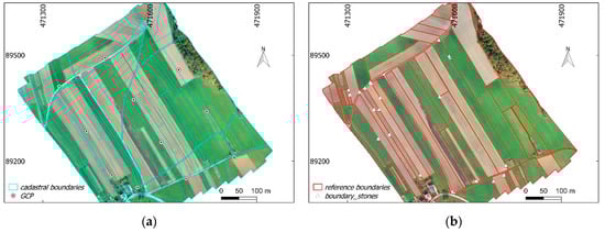
Figure 1.
(a) Cadastral map and ground control points (GCPs). (b) Manually delineated object visible boundaries used as reference data to determine the detection/extraction quality. (a,b) Overlaid on UAV orthoimage of Ponova vas, Slovenia (EPSG 3794).
2.2. Reference data
The current cadastral map for the selected area was retrieved from the e-portal of the Slovenian Surveying and Mapping Authority, which is an online platform for requesting official cadastral data [42]. The cadastral map was overlaid on the UAV orthoimage (Figure 1a). The visual interpretation of the combined dataset showed immediately that the cadastral map does not correspond with the visible objects that indicate land possession (land cover) boundaries (roads, agricultural field outlines) on the UAV orthoimage. From the initial analyses, it appeared that only 8% of cadastral boundaries correspond with the manually digitized visible boundaries (at 25 cm tolerance). This is because the current official cadastral map was created by digitizing previous analog cadastral maps whose origin goes back in the first half of 19th century. Due to the underestimated need for cadastral map updating as well as due to the land reforms in the 20th century (i.e., land nationalization and denationalization) the current possession land boundaries do not correspond with cadastral boundaries. Considering this, as reference data, manually digitized boundaries were used instead of the official cadastral data, as the aim of this research is to automatically delineate visible object boundaries from a UAV orthoimage and, at the same time, study the potential of the ENVI FX solution for the automatic detection of visible boundaries. Moreover, during the manual digitization of reference boundaries, some white stones considered as possession boundary signs were used as a guide for proper digitization (Figure 1b). The placement of white stones is a common practice in the selected study area, and for this reason, they were considered as reliable information during the manual digitization. In addition, the confidence in white stones as boundary signs is based on the authors’ experiences in professional cadastral surveying.
2.3. Visible Boundary Delineation Method and Workflow
2.3.1. ENVI Feature Extraction (FX)
The investigated tool, ENVI FX, is a combined process of image segmentation and classification. The focus of this study is only at image segmentation and calculating spatial attributes for each segmented object [41]. In addition to spatial attributes, spectral and textural attributes are often used by users for further image classification analysis.
The first step, image segmentation, is based on the technique developed by Jin [43] and involves calculating a gradient map, calculating cumulative distribution function, modification of the gradient map by defining a scale level, and segmentation of a modified gradient map by using the Watershed Transform [44]. A gradient is calculated for each band of the image. The ENVI FX module uses two approaches: edge method and intensity. The edge method calculates a gradient map using the Sobel edge detection algorithm [44]. The Intensity method converts each pixel to a spectral intensity value by averaging it across the selected image bands [44]. The edge method is used for detecting features with distinct boundaries and is considered in this study. In contrast, the Intensity method is suitable for digital elevation models, images of gravitational potential and images of electromagnetic fields [44]. After a gradient map is calculated, a density function of gradients over the whole map is calculated in the form of a cumulative relative histogram [43]. Once the cumulative distribution function has been calculated, it can be used along with the gradient map to calculate the gradient scale space [43]. The gradient map can be modified by changing the scale level. The scale level is the relative threshold on the cumulative relative histogram from which the corresponding gradient magnitude can be determined [43]. For example, at a scale level of 50, the lowest 50 percent of gradient magnitude values are discarded from the gradient image [44]. Increasing the scale level results in fewer segments and keeps objects with the most distinct boundaries [41]. Once the scale level is selected the Watershed Transform algorithm is applied to the modified gradient map. The Watershed Transform is based on the concept of hydrologic watersheds [22,35]. In digital imagery, the same process can be similarly explained as the darker a pixel, the lower its "elevation" (minimum pixel). The algorithm categorizes a pixel by increasing the greyscale value, then begins with the minimum pixels and "floods" the image, dividing the image into objects with similar pixel intensities. The result is a segmented image and each segmented object is assigned with a mean spectral value of all the pixels that belong to that object [44].
The second step is merging. This step aggregates over-segmented areas by using the ENVI FX default full Lambda schedule algorithm. The algorithm is meant to aggregate object outlines within larger, textured areas, such as trees and, fields, based on a combination of spectral and spatial information [41,45]. The merge level represents the threshold Lambda value. Merging occurs when the algorithm finds a pair of adjacent objects such that the merging cost is less than a defined threshold Lambda value—if the merge level is set to 20, it will merge adjacent objects with the lowest 20 percent of Lambda values [45]. When a merge level of 0 is selected no merging will be performed. In this step, the selection of Texture Kernel Size is optional, i.e., the size of a moving box centered over each pixel value. The ENVI FX default Texture Kernel Size is 3, and the maximum is 19 [45].
The final step is the export of object boundaries in a vector format and a segmented image in a raster format. Moreover, each extracted object consists of spatial, spectral, and texture information in the attribute table [41].
2.3.2. Visible Boundary Delineation Workflow
The visible boundary delineation workflow (Figure 2) consists of four main steps. In the following, each workflow step is described in detail with additional comments based on our own preliminary studies aiming to understand and justify the selection of the parameters and algorithms used. The first and second steps were implemented in ENVI 5.5 image analysis software [46] by using the ENVI FX [47] tool. The other steps were implemented using QGIS [48] and GRASS [49] functions.
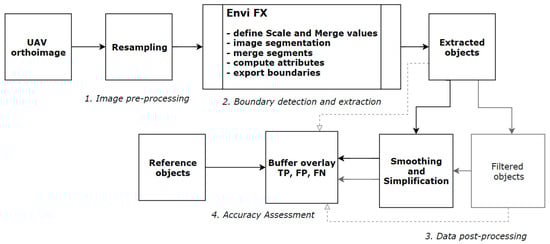
Figure 2.
Cadastral mapping workflow based on the automatic detection and extraction of visible boundaries from UAV imagery.
- Image pre-processing: The first step is resampling the UAV orthoimage. The UAV orthoimage was resampled from 2 cm to lower spatial resolutions—25 cm, 50 cm and 100 cm ground sample distances (GSD). The selected GSDs allowed the identification of the impact of different GSDs on the results of automatic boundary extractions. The pixel average method was used for resampling the UAV orthoimage as it provides a smoother image. In addition, further resampling methods (nearest neighbor and bilinear) were tested and did not provide significant differences in the number of automatic object boundary extractions—at higher scale and merge levels of the ENVI FX algorithm. The resampling step was also applied in [26], to make transferable the investigated method to a UAV orthoimage for cadastral mapping purposes. In addition, extracting objects from a UAV orthoimage of lower spatial resolution is computationally less expensive.
- Boundary detection and extraction: The ENVI FX module was applied to each down-sampled UAV orthoimage. The detection and extraction of visible boundaries from the UAV orthoimage was based on the ENVI FX scale and merge level values. The texture kernel size was set to default, i.e., 3. In addition, further object extractions were tested at the highest texture kernel size and no differences in the number and locations of extracted objects were identified. Scale level values ranged from 50 to 80 and merge level values from 50 to 99. The initial incremental value for both scale and merge levels was 10. In cases where a jump in the total number of extracted objects was detected the incremental value was dropped for both scale and merge levels. In order to identify the optimal scale and merge values for the detection and extraction of visible objects for cadastral mapping, all possible range values of scale and merge combinations were tested. For each extraction information about the total number of extracted objects and processing time was stored. This resulted in 50 boundary maps for each resampled UAV orthoimage. The boundary map consisted of extracted objects (polygon-based), which were in digital vector format.
- Data post-processing: The process included two steps: (i) the filtering of extracted objects, and (ii) the simplification of extracted objects. (i) The minimum object area and the total number of objects identified in the reference data (Figure 1b) were used to determine optimal scale and merge levels. The minimum reference object area was 204 m2, and the total number of objects was 68. All extracted objects that were smaller than the minimum object area from reference data were filtered out (removed). The total number of remaining objects was compared with the total number of objects from the reference data and the tolerance of +/- 10 objects was set—those parameters that produced numbers of objects that were closest to those found in the reference data, i.e., within defined tolerance, were deemed optimal. The boundary maps from which smaller objects were removed were labeled as filtered objects. The output of filtered objects consisted of holes, i.e., due to polygon-based geometry of objects, which were mostly present either in the forest or individual trees and are of less relevance for cadastral applications—a boundary between adjacent objects belongs to both. (ii) Extracted and filtered object boundaries were smoothed and simplified to be used for the interpretation of possession boundaries aiming to support a cadastral mapping (i.e., land plot restructuring in this case, as the situation requires a new cadastral survey or land consolidation). The smoothing of extracted/filtered object boundaries was done by using the Snakes algorithm [49]. The Douglas–Peucker algorithm was applied to the smoothed object boundaries in order to further simplify the object boundaries [22,49]. These objects both smoothed and simplified were labeled as simplified extracted/filtered objects.
- Accuracy assessment: The accuracy assessment was object-based since the results were in vector format. The buffer overlay method was used for accuracy assessment. The method is described in detail in Heipke et al. [50]. The accuracy assessment was based on computing the percentages of extracted (or reference) boundary lengths which overlapped within a buffer polygon area generated around the reference (or extracted) boundaries (Figure 3) [50]. To determine the completeness, correctness, and quality of extracted boundaries, calculated boundary lengths of true positives (TP), false positives (FP), and false negatives (FN) were used. The completeness refers to the percentage of reference boundaries which lie within the buffer around the extracted boundaries (matched reference). The correctness refers to the percentage of extracted boundaries, which lie within the buffer around the reference boundaries (matched extraction). The accuracy assessment was performed on buffer widths of 25 cm, 50 cm, 100 cm, and 200 cm. The selection of buffer widths is in line with other studies and was based on the most common tolerances regarding boundary positions in land administration, especially for rural areas [26,27]. The percentage indicating the overall quality was generated from the previous two by dividing the length of the matched extractions with the sum of the length of extracted data and the length of unmatched reference [50]. The accuracy assessment was applied to automatic extracted objects, simplified extracted objects, filtered objects, and simplified filtered objects (Figure 2).
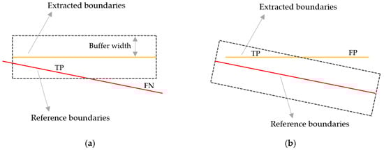 Figure 3. Object-based accuracy assessment method—buffer overlaying method. (a) Matched reference. (b) Matched extraction. (a,b) Calculation of boundary lengths of true positives (TP), false positives (FP) and false negatives (FN) (Adapted from [50]).
3. Results
Resampling the UAV orthoimage to a lower spatial resolution, i.e., a larger value of GSD, resulted in fewer and faster extractions of object boundaries compared to the number of extracted object boundaries generated at the original size of the UAV orthoimage. The processing time for one boundary map was 1–2 min. A larger GSD, at the same scale and merge values, resulted in fewer boundary extractions (Table 2, Figure 4 and Figure 5).
Table 2.
Ground sample distance (GSD) and number of pixels after image pre-processing.
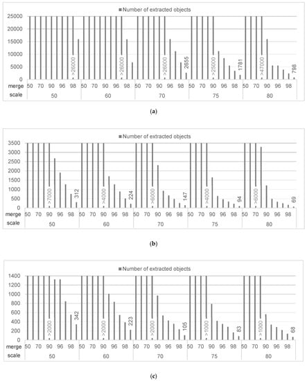
Figure 4.
Scale/merge level and number of extracted objects from the resampled UAV orthoimages (a) ground sample distance (GSD) 25 cm, (b) GSD 50 c, and (c) GSD 100 cm. (a–c) Grey labels—number of extracted objects outside the range, black labels—the lowest number of extracted objects per scale and merge parameter value.
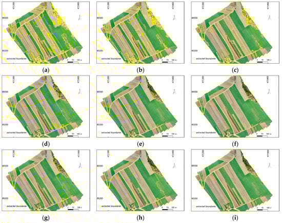
Figure 5.
(a–i) Examples of extracted boundary maps. (a–c) GSD 25 cm; (d–f) GSD 50 cm, and (g–i) GSD 100 cm. (a,d,g) Extracted objects at scale 70 and merge 99. (b,e,h) Extracted objects at scale 75 and merge 99. (c,f,i) Extracted objects at scale 80 and merge 99.
A lower scale level and merge level resulted in a higher number of extracted object boundaries for each resampled UAV image. A higher scale and merge level resulted in fewer extracted boundaries (Figure 4). In general, for all resampling, the biggest drop in the number of extracted object boundaries was at scale level values within the range from 70 to 80, and merge level values within the range from 95 to 99 (Figure 4). The incremental value of 1, for merge level 95–99, turned out to be very sensitive in dropping the number of extracted object boundaries (Figure 4a–c).
The optimal scale and merge levels for an automatic boundary delineation were investigated by filtering out the total number of extracted objects with the minimum area of objects from the reference data. The results of this filtering approach are presented in Figure 6. The results showed that for the UAV orthoimages of higher spatial resolutions, namely a GSD of 25 cm, the optimal algorithm values for cadastral mapping resulted in 80 for scaling and from 95 to 99 for merging. In contrast, for the UAV orthoimages having a GSD of 50 cm and a GSD of 100 cm, the common optimal scale level values were 70–80 and merge level 95–98 (Figure 6). Some exceptions were observed for a GSD of 50 cm, where the scale level was 50, 60, and merge level to its maximum. In general, the results showed that the optimal scale and merge level values suitable for cadastral mapping range from 70 to 80 and from 95 to 99, respectively (examples in Figure 5). The optimal scale and merge level values appeared similar as in the investigation of the influence of different GSDs in extracting objects.
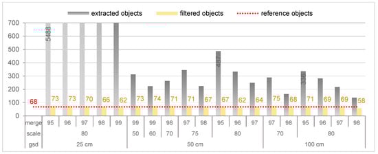
Figure 6.
Comparison in the number of extracted and filtered objects using different scale and merge parameter values, to the number of objects identified in the reference data set.
For further analysis, optimal extracted objects with scale level 80 and merge level 95 for three GSDs of UAV orthoimages were selected (Figure 7a,c,e). The selection was based on common scale and merge levels for three GSDs as well on the highest number of filtered objects per GSD (Figure 6). The filtering approach was additionally applied to the selected optimal extracted objects, i.e., with scale level 80 and merge level 95, to remove objects under the minimum reference object area (Figure 7b,d,f).
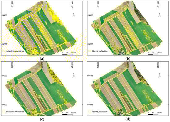
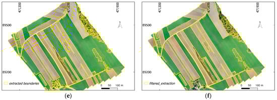
Figure 7.
(a,c,e) Extracted objects at scale level 80 and merge level 95 for (a) GSD 25 cm, (c) GSD 50 cm, and (e) GSD 100 cm. (b,d,f) Filtered objects of scale level 80 and merge level 95 based on minimum object area from the reference data.
A simplification algorithm was applied to both extracted objects and filtered objects. The results showed that if extracted objects are smoothed and smoothed objects are later simplified, the localization of simplified objects is almost equal to that of the extracted ones (Figure 8). The initial tests show that possible shifts in location are possible when a direct implementation of the simplification algorithm to extracted visible objects is used.
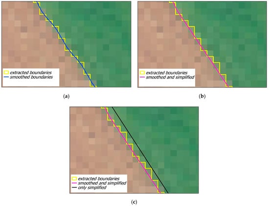
Figure 8.
(a) Extracted objects smoothed by making use of the Snakes algorithm. (b) Simplification of extracted objects by making use of the Snakes smoothing algorithm and Douglas–Peucker simplification algorithm. (c) Extracted objects simplified with Douglas–Peucker algorithm (in black) and compared to object simplifications on (b).
The buffer overlay method was used for the accuracy assessment. The accuracy assessment method was applied to the extracted objects, simplified extracted objects, filtered objects and simplified filtered objects. The results show that there is no significant difference in accuracy assessment results when comparing extracted and simplified objects (Table 3, Table 4, and Table 5). At a buffer width of 2 m, a GSD of 50 cm and a GSD of 100 cm provide a higher percentage of correctly extracted objects compared to a GSD of 25 cm. The percentage of correctly extracted objects was 66% for both a GSD of 50 cm and a GSD of 100 cm (Table 4 and Table 5). However, the filtering approach contributed to the increased correctness (decreased completeness) and overall quality, for all GSDs. From the filtered objects, the best results for correctness were recorded at a GSD of 50 cm (Figure 9). The percentage indicated the correctness was 77%, while for the completeness it was 67%.
Table 3.
Accuracy assessment of boundary extractions for a GSD of 25 cm, scale 80, merge 95.
Table 4.
Accuracy assessment of boundary extractions for a GSD of 50 cm, scale 80, merge 95.
Table 5.
Accuracy assessment of boundary extractions for a GSD of 100 cm, scale 80, merge 95.
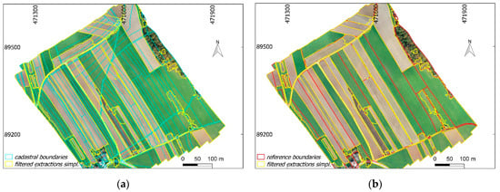
Figure 9.
(a,b) Filtered objects of scale level 80 and merge level 95—simplified, compared with (a) cadastral map and (b) manually delineated visual object boundaries used as reference data.
4. Discussion
4.1. The Developed Workflow
The developed workflow aimed to provide a solution for UAV-based cadastral mapping using automatic visible boundary extraction with the ENVI FX module (Figure 2). The developed workflow consisted of four steps: (i) image pre-processing, (ii) boundary detection and extraction, (iii) data post-processing, and (iv) accuracy assessment.
The first workflow step includes resampling of a UAV orthoimage. Here, the results of our case study showed that larger GSDs provided faster and fewer extractions of visible object boundaries compared to the original GSD of a UAV orthoimage. For higher spatial resolutions, i.e., smaller GSDs, considering the selected Scale level and Merge level values, the total number of extracted objects was higher.
The second step, which includes object boundary detection and extraction, is dependent on the scale and merge level. The results, presented in Figure 4, showed that lower values of scale and merge levels resulted in a higher number of extracted objects, which led to over-segmentation by reaching thousands of extracted objects. Considering the total number of the reference objects, it is important to note that a scale and a merge level that provide object extractions close to the total number of objects from reference data are important for automatic delineation of visible cadastral boundaries.
The following step, data post-processing, aimed to investigate optimal scale and merge levels and to simplify the extracted objects. The optimal values based on a filtering approach showed that for all tested GSDs in this study, most suitable scale and merge level values for automatic delineation of visible cadastral boundaries were 70–80 and 95–99, respectively. These values can be considered as optimal scale and merge levels for rural areas in general or areas with characteristics similar to the study area of this research. However, to validate the proposed workflow and optimal Scale and Merge levels in areas with different characteristics, such as areas with a larger number of buildings or areas with trees covering parts of boundaries, further experiments are needed. Hence, the scale and merging levels appropriate for cadastral mapping have been determined and this step can be skipped from the workflow step of data post-processing (Figure 2). The use of the Snakes algorithm for smoothing and the Douglas–Peucker algorithm for simplifying has been shown to be very effective (Figure 8a,b). This approach, when combining both smoothing and simplification algorithms, gives better results in terms of a simplified boundary position compared to directly implementing the Douglas–Peucker simplification algorithm, where undesired shifting in boundary position was observed (Figure 8c). In [22], it was reported that the direct implementation of the Douglas–Peucker algorithm was used as a post-processing method in many papers to improve the output by optimizing the shape of objects. However, the simplification approach applied in this study was not examined in the previous papers.
The final step of the workflow was accuracy assessment (see also Section 4.2). The accuracy assessment was based on the buffer overlay method. By increasing the width of the buffer, more extracted boundaries appear to be within the buffer area, which impacts the completeness, correctness, and the overall quality—larger the buffer, the better the results. To have a uniform assessment for all tested GSDs the results were compared at a buffer distance of 2 m. From the reviewed publications presented in Section 1.2, a buffer width of 2 m was also applied in [26,27,28] as most suitable for the presentation of accuracy assessment results and to avoid uncertainties from resampling effects. However, for comparison to cadastral data, buffer widths should be based on local accuracy requirements [26].
The workflow developed, overall, is in accordance with the general workflow for the cadastral mapping based on suitable computer vision methods for automatic visible boundary extraction provided in [22]. In addition, it provides an additional step and method in data post-processing, such as filtering out irrelevant and small objects from the boundary map, which improves overall quality assessment. Furthermore, it suggests a combined approach for the simplification of extracted object boundaries.
4.2. Quality Assessment
Bringing the scale and merge levels to the maximum resulted in some unextracted and fewer visible objects for the whole extent of the image. Although some of the visible objects were left unextracted, the maximum scale and merge level enabled the detection of a group of objects such as a group of tree boundaries, especially at GSDs of 50 cm and 100 cm (Figure 5f,i). In both cases, the balance between completeness and correctness was hard to achieve. This issue was also reported in [26,28]. For this reason, the filtering approach was applied. It was based on the minimum object size as well as on the total number of the objects, both defined based on the reference data. This allowed us to reduce the risk that some of the visible object boundaries remained unextracted as well as over-segmented.
The optimal scale level of 80 and a merge level of 95, were chosen for all three GSDs, to investigate the impact of the same scale and merge level in different resampling. The selection was based on common scale and merge levels per GSD (Figure 6). However, this does not mean that the chosen scale and merge level provided the best object boundary extraction for each of the GSDs. For instance, for small GSDs, the correctness of extracted boundaries is higher at the maximum scale and merge levels (e.g., Figure 5c). For the same scale and merge level, the correctness grows significantly from a GSD of 25 cm to a GSD of 50 cm. The correctness for a GSD of 100 cm was almost equal to the one for a GSD of 50 cm. Considering that more optimal scale and merge levels were applicable for a GSD of 50 cm (Figure 6) and the difference insignificant when compared to the results obtained for a GSD of 100 cm, a GSD of 50 cm appeared to be better in detecting visible boundaries compared to the other two GSDs.
The quantitative method applied for accuracy assessment to automatically extracted objects, filtered objects and to their simplifications, showed that there was no significant difference between extracted objects and simplified objects. This result indicates that the method applied for simplification can be considered appropriate, i.e., the original location of extracted objects was maximally maintained. Although there was no difference in accuracy assessment, the simplification of extracted (or filtered) objects is significant for proper cadastral mapping. Cadastral boundaries usually are defined by straight lines with fewer vertices.
The percentage of suitable extracted boundaries (compared to reference data), for a scale level of 80 and a merge level of 95, resulted in 74% for the assessment of the completeness and 66% for the assessment of the correctness for the extracted object boundaries having a GSD of 50 cm. However, the filtering approach strongly influenced the accuracy assessment. For filtered extractions, the level of completeness was 67%, and the level of correctness was 77%. These results show that the filtering approach increased the correctness of automatically extracted boundaries, and it reaches almost 80% (Table 4). This was due to filtering out small object boundaries from the boundary map. The excluded small objects were mostly present in tree and built-up areas on the UAV orthoimage, i.e., only outlines of group objects were retained (Figure 7c,d). In road extractions, the achieved values for extractions are around 85% for correctness and around 70% for completeness to be of real practical importance [26,34]. Such percentages can hardly be achieved by the workflow developed for automatic delineation of all visible boundaries since the morphology of cadastral boundaries is usually more complex and not all cadastral boundaries are visible, unlike road boundaries.
The accuracy assessment was based on the manually delineated boundaries, which were defined as reference data (Figure 1b). The visible boundaries were manually delineated on the ground truth UAV orthoimage. It is argued that manually delineated boundaries influence the overall results of the accuracy assessment since different human operators might digitize differently [26]. However, in the selected case study, most of the object boundaries were sharp and the presence of white stones at outlines of the agricultural field contributed to the objectivity of manual digitalization. In addition, the real cadastral data could not be used since they did not correspond with the object boundaries on the image (Figure 1a) and it would not have been possible to outline the potential of the ENVI FX. However, the approach of automatic extraction of visible boundaries is case dependent. To reliably avoid the influence of manually digitized reference data, the following studies should consider a case study where the cadastral map is up to date.
4.3. Strengths and Limitations of the Automatic Extraction Method Used
The ENVI FX module handled the full extent of the resampled UAV orthoimages, and no additional image tiling or image conversions were required. ENVI FX provided closed object boundaries directly in vector format, topologically correct polygons. Therefore, no additional image post-processing step, such as vectorization of detected object boundaries, was needed (Figure 5). Thus, the visible object boundaries generated can be directly used for further processing and analysis within geographic information systems (GIS). Additionally, the final output consists of spatial, spectral and textural attributes which are assigned automatically to each extracted object and saved in the attribute table. The vectorized and geo-referenced visible object boundaries, as interpreted in this research, are crucial in cadastral applications especially for the purposes of land plot boundary delineations. Overall, ENVI FX has the potential to automatically delineate visible cadastral boundaries, especially in rural areas.
A comparison of the results regarding the accuracy assessment obtained in this study and the accuracies obtained in the studies [26,27,28] cannot be done at this time for a number of reasons. First, not all the reviewed feature extraction methods have been applied to UAV imagery. Second, different UAVs may provide different quality of orthoimages. Third, the nature, size, location, and the characteristics of the study objects are far too different. In order to make a reliable comparison on accuracy assessments of different feature extraction methods, first of all, each method has to be studied individually and later tested at the same study area(s). However, the image processing approach of different feature extractions methods may be comparable.
From the reviewed feature extraction methods that have already been applied for detection of visible cadastral boundaries, it can be seen that the MRS method, ESP method, and mean-segmentation method also do not require further image tiling and the final output of the boundary map was in vector format [27,28]. In contrast, vectorization of detected object boundaries was needed for the gPb contour detection method. In addition, it was reported that the method is inapplicable when processing UAV images of more than 1000 pixels in width and height [26]. Similar issues regarding the vectorization of detected object boundaries were reported in [38], where Canny and Sobel edge detection algorithms were used. In order to obtain topologically correct polygons, an additional feature extraction method was used aiming to connect the edges.
ENVI FX allowed some shadow areas in the UAV orthoimage to be extracted as boundaries; however, these do not represent real boundaries in the field. In order to minimize the influence of shadows on feature extraction, it is recommended to capture images in the local time where the solar zenith angle has the smallest possible value. However, the solar zenith angle depends on the geographic location of the study area. Additionally, some other factors such as weather conditions also influence the quality of captured images. To avoid such issues, it is preferable to capture images on a cloudy day without wind. Although ENVI FX has proved to be efficient, one of its limitations is that it is not an open-source tool like mean-shift segmentation, gPb contour detection, Canny, and Sobel, which might be a reason why it is not often used in the land surveyor community. In addition, the extracted objects from the resampled UAV orthoimages were following the pixel borders and further shape simplification was required to make them comparable to spatial units in cadastral applications.
Considering that the morphology of cadastral boundaries is complex [7], compared to physical boundaries, such as boundaries of roads or rivers, delineation of cadastral boundaries cannot be fully automated at this time, and additionally, the verification of the results has to be done with the participation of landowners and other land rights holders. The limitations on extracting only visible object boundaries lie in the fact that not all visible boundaries (land cover boundaries) represent cadastral boundaries (land right boundaries). For instance, when two agricultural cadastral units leased to the same farmer are farmed as one unit, and vice versa. However, visible object boundaries which coincide with the land right boundaries can be automatically detected and used in cadastral applications. In addition, the UAV-based spatial data acquisition is usually affected by special operational regulations that restrict the use of this technology, in particular in urban areas [18].
4.4. Applicability of the Developed Workflow
The developed workflow provided geo-referenced boundary maps in a format compliant with the formats that are used in GIS environments. This shows that the extracted objects can be easily transferable, and applicable in GIS for cadastral purposes. In cases where cadastral maps are rarely present and the concept of fit-for-purpose cadastre is in place, the workflow, with the selected method for automatic extraction of visible boundaries, shows the potential for the automation of the visible cadastral boundary delineation procedure [1]. Thus, the approach developed generally contributes to the acceleration and facilitation of the creation of cadastral maps (Figure 9b), especially in developing countries, where general boundaries are accepted, and positional accuracy is of lesser importance [25]. However, the approach is suitable for the areas where the boundaries of physical objects are visibly detectable on a UAV orthoimage, for instance, in rural areas. The workflow might be applicable for both the creation and updating/revision of cadastral maps, similar to the manual delineations of cadastral boundaries on a UAV orthoimage. In addition, the workflow developed might lower the costs and time compared to the manual delineation of cadastral boundaries, especially in rural areas [26].
Furthermore, in developed countries, the approach based on automatic extraction of visible boundaries might be used for a revision of current cadastral maps (Figure 9a). In this case, the extracted visible boundaries can be used as a basis for a new cadastral survey or land rearrangements, depending on the discrepancy between cadastral maps and land possession (as shown in the case study). Although the beneficiaries agree with the visible boundaries, if higher accuracy is required, the revised objects (spatial units) can later be manually delineated from a UAV orthoimage or re-surveyed with ground-based surveying techniques. It must be emphasized that the extracted visible boundaries, both for the creation of cadastral maps and updating, should be inspected by the local community and all beneficiaries (landowners, other land rights holders) in order to be legally validated.
5. Conclusions
The overall aim of this study was to provide an UAV-based cadastral mapping workflow based on the ENVI FX module for automatic detection of visible boundaries. The study first investigated, which processing steps are required for a cadastral mapping workflow following the potential and limitations of the ENVI FX for automatic visible boundary detection and extraction.
The results showed that more correct visible object boundaries, suitable for the interpretation of land cover (cadastral) boundaries, were extracted at larger values of GSD. In addition, the identified optimal scale and merge levels for detection and extraction of visible cadastral boundaries were between 70 and 80 and 95 and 99, respectively. The identification of the optimal parameters for cadastral mapping was based on the defined minimum object area and the total number of objects from the reference data using the so-called filtering approach. The filtering approach contributed to the increased correctness of automatically extracted boundaries. The best results were recorded at the resampled UAV orthoimage with a GSD of 50 cm, and the percentage of correctness indicated was 77%, while for the completeness it was 67%. It must be emphasized that the workflow developed is applicable mostly for rural areas where the number of visible boundaries is higher compared to complex urban areas.
The workflow can be used in developing countries to accelerate and facilitate the creation of cadastral maps aiming to formalize a land tenure system and guarantee legal security to land rights holders. In developed countries, the extracted visible boundaries based on this workflow might be used for efficient revision of existing cadastral maps. However, in both cases, the extracted visible boundaries have to be validated by landowners and other beneficiaries. The extraction of visible objects can be considered as only one step in the facilitation of cadastral mapping, as extracting these is not enough for complete and correct cadastral mapping. It is worth highlighting that cadastral boundaries may, in fact, be completely inside the property and that some boundaries between properties may not be clearly visible. In order to use the proposed workflow in the cadastral domain, the approach can be expanded. Additional steps should focus on methods for the possible involvement of current landowners in the process of cadastral mapping. The extension of the current workflow is one of the aims of the authors’ further research.
Author Contributions
Conceptualization, B.F. and A.L.; methodology, B.F., K.O. and A.L.; software, B.F.; validation, B.F., K.O. and A.L.; formal analysis and data processing, B.F.; investigation, B.F.; resources, B.F., A.L., K.O. and M.K.F.; writing—original draft preparation, B.F.; writing—review and editing, B.F., A.L., K.O. and M.K.F.; visualization, B.F.; supervision, A.L.
Funding
The authors acknowledge the financial support of the Slovenian Research Agency (research core funding No. P2-0406 Earth observation and geoinformatics).
Acknowledgments
We acknowledge Klemen Kozmus Trajkovski and Albin Mencin for capturing the UAV data and for the technical support during the fieldwork.
Conflicts of Interest
The authors declare no conflict of interest.
Abbreviations
The following abbreviations are used in this article:
| DSM | Digital Surface Model |
| ESP | Estimation of Scale Parameter |
| FIG | International Federation of Surveyors |
| FN | False Negative |
| FP | False Positive |
| FX | ENVI Feature Extraction |
| GCP | Ground Control Point |
| GIS | Geographic Information System |
| GNSS | Global Navigation Satellite System |
| gPb | Global Probability of Boundary |
| GSD | Ground Sample Distance |
| HRSI | High-Resolution Satellite Imagery |
| MRS | Multi-Resolution Segmentation |
| PDOP | Position Dilution of Precision |
| RMSE | Root-Mean-Square-Error |
| RTK | Real-Time Kinematic |
| SLIC | Simple Linear Iterative Clustering |
| TP | True Positive |
| UAV | Unmanned Aerial Vehicle |
References
- Enemark, S. International Federation of Surveyors. In Fit-For-Purpose Land Administration: Joint FIG/World Bank Publication; FIG: Copenhagen, Denmark, 2014; ISBN 978-87-92853-10-3. [Google Scholar]
- Luo, X.; Bennett, R.; Koeva, M.; Lemmen, C.; Quadros, N. Quantifying the Overlap between Cadastral and Visual Boundaries: A Case Study from Vanuatu. Urban Sci. 2017, 1, 32. [Google Scholar] [CrossRef]
- Zevenbergen, J. A Systems Approach to Land Registration and Cadastre. Nord. J. Surv. Real Estate Res. 2004, 1, 11–24. [Google Scholar]
- Simbizi, M.C.D.; Bennett, R.M.; Zevenbergen, J. Land tenure security: Revisiting and refining the concept for Sub-Saharan Africa’s rural poor. Land Use Policy 2014, 36, 231–238. [Google Scholar] [CrossRef]
- Land Administration for Sustainable Development, 1st ed.; Williamson, I.P., Ed.; ESRI Press Academic: Redlands, CA, USA, 2010; ISBN 978-1-58948-041-4. [Google Scholar]
- Zevenbergen, J.A. Land Administration: To See the Change from Day to Day; ITC: Enschede, The Netherlands, 2009; ISBN 978-90-6164-274-9. [Google Scholar]
- Luo, X.; Bennett, R.M.; Koeva, M.; Lemmen, C. Investigating Semi-Automated Cadastral Boundaries Extraction from Airborne Laser Scanned Data. Land 2017, 6, 60. [Google Scholar] [CrossRef]
- Enemark, S. Land Administration and Cadastral Systems in Support of Sustainable Land Governance—A Global Approach. In Proceedings of the Re-Engineering the Cadastre to Support E-Government, Tehran, Iran, 4–26 May 2009. [Google Scholar]
- Maurice, M.J.; Koeva, M.N.; Gerke, M.; Nex, F.; Gevaert, C. A Photogrammetric Approach for Map Updating Using UAV in Rwanda. Available online: https://bit.ly/2FyhbEi (accessed on 25 June 2019).
- Wayumba, R.; Mwangi, P.; Chege, P. Application of Unmanned Aerial Vehicles in Improving Land Registration in Kenya. Int. J. Res. Eng. Sci. 2017, 5, 5–11. [Google Scholar]
- Ramadhani, S.A.; Bennett, R.M.; Nex, F.C. Exploring UAV in Indonesian cadastral boundary data acquisition. Earth Sci. Inform. 2018, 11, 129–146. [Google Scholar] [CrossRef]
- Mumbone, M.; Bennet, R.; Gerke, M. Innovations in Boundary Mapping: Namibia, Customary Lands and UAVs. In Proceedings of the Linking Land Tenure and Use for Shared Prosperity, Washington, DC, USA, 23–27 March 2015; p. 22. [Google Scholar]
- Volkmann, W.; Barnes, G. Virtual Surveying: Mapping and Modeling Cadastral Boundaries Using Unmanned Aerial Systems (UAS). In Proceedings of the FIG Congress 2014, Kuala Lumpur, Malaysia, 16–21 June 2014; p. 13. [Google Scholar]
- Rijsdijk, M.; van Hinsbergh, W.H.M.; Witteveen, W.; ten Buuren, G.H.M.; Schakelaar, G.A.; Poppinga, G.; van Persie, M.; Ladiges, R. Unmanned Aerial Systems in the process of Juridical verification of Cadastral borde. ISPRS Int. Arch. Photogramm. Remote Sens. Spat. Inf. Sci. 2013, XL-1/W2, 325–331. [Google Scholar] [CrossRef]
- Mesas-Carrascosa, F.J.; Notario-García, M.D.; Meroño de Larriva, J.E.; Sánchez de la Orden, M.; García-Ferrer Porras, A. Validation of measurements of land plot area using UAV imagery. Int. J. Appl. Earth Obs. Geoinf. 2014, 33, 270–279. [Google Scholar] [CrossRef]
- Manyoky, M.; Theiler, P.; Steudler, D.; Eisenbeiss, H. Unmanned Aerial Vehicle in Cadastral Applications. ISPRS Int. Arch. Photogramm. Remote Sens. Spat. Inf. Sci. 2012, XXXVIII-1/C22, 57–62. [Google Scholar] [CrossRef]
- Kurczynski, Z.; Bakuła, K.; Karabin, M.; Kowalczyk, M.; Markiewicz, J.S.; Ostrowski, W.; Podlasiak, P.; Zawieska, D. The posibility of using images obtained from the UAS in cadastral works. ISPRS Int. Arch. Photogramm. Remote Sens. Spat. Inf. Sci. 2016, XLI-B1, 909–915. [Google Scholar] [CrossRef]
- Cramer, M.; Bovet, S.; Gültlinger, M.; Honkavaara, E.; McGill, A.; Rijsdijk, M.; Tabor, M.; Tournadre, V. On the use of RPAS in National Mapping—The EuroSDR point of view. ISPRS Int. Arch. Photogramm. Remote Sens. Spat. Inf. Sci. 2013, XL-1/W2, 93–99. [Google Scholar] [CrossRef]
- Binns, B.O.; Dale, P.F. Cadastral Surveys and Records of Rights in Land. Available online: http://www.fao.org/3/v4860e/v4860e03.htm (accessed on 20 March 2019).
- Watts, A.C.; Ambrosia, V.G.; Hinkley, E.A. Unmanned Aircraft Systems in Remote Sensing and Scientific Research: Classification and Considerations of Use. Remote Sens. 2012, 4, 1671–1692. [Google Scholar] [CrossRef]
- Colomina, I.; Molina, P. Unmanned aerial systems for photogrammetry and remote sensing: A review. ISPRS J. Photogramm. Remote Sens. 2014, 92, 79–97. [Google Scholar] [CrossRef]
- Crommelinck, S.; Bennett, R.; Gerke, M.; Nex, F.; Yang, M.; Vosselman, G. Review of Automatic Feature Extraction from High-Resolution Optical Sensor Data for UAV-Based Cadastral Mapping. Remote Sens. 2016, 8, 689. [Google Scholar] [CrossRef]
- Heipke, C.; Woodsford, P.A.; Gerke, M. Updating geospatial databases from images. In Advances in Photogrammetry, Remote Sensing and Spatial Information Sciences: 2008 ISPRS Congress Book; Baltsavias, E., Li, Z., Chen, J., Eds.; CRC Press: London, UK, 2008. [Google Scholar]
- Bennett, R.; Kitchingman, A.; Leach, J. On the nature and utility of natural boundaries for land and marine administration. Land Use Policy 2010, 27, 772–779. [Google Scholar] [CrossRef]
- Zevenbergen, J.; Bennett, R. The visible boundary: More than just a line between coordinates. In Proceedings of the GeoTech Rwanda, Kigali, Rwanda, 18–20 November 2015; pp. 1–4. [Google Scholar]
- Crommelinck, S.; Bennett, R.; Gerke, M.; Yang, M.; Vosselman, G. Contour Detection for UAV-Based Cadastral Mapping. Remote Sens. 2017, 9, 171. [Google Scholar] [CrossRef]
- Wassie, Y.A.; Koeva, M.N.; Bennett, R.M.; Lemmen, C.H.J. A procedure for semi-automated cadastral boundary feature extraction from high-resolution satellite imagery. J. Spat. Sci. 2018, 63, 75–92. [Google Scholar] [CrossRef]
- Kohli, D.; Crommelinck, S.; Bennett, R. Object-Based Image Analysis for Cadastral Mapping Using Satellite Images. In Proceedings of the International Society for Optics and Photonics, Image Signal Processing Remote Sensing XXIII; SPIE. The International Society for Optical Engineering: Warsaw, Poland, 2017. [Google Scholar]
- Kohli, D.; Unger, E.-M.; Lemmen, C.; Koeva, M.; Bhandari, B. Validation of a cadastral map created using satellite imagery and automated feature extraction techniques: A case of Nepal. In Proceedings of the FIG Congress 2018, Istanbul, Turkey, 6–11 May 2018; p. 17. [Google Scholar]
- Singh, P.P.; Garg, R.D. Road Detection from Remote Sensing Images using Impervious Surface Characteristics: Review and Implication. ISPRS Int. Arch. Photogramm. Remote Sens. Spat. Inf. Sci. 2014, XL-8, 955–959. [Google Scholar] [CrossRef]
- Kumar, M.; Singh, R.K.; Raju, P.L.N.; Krishnamurthy, Y.V.N. Road Network Extraction from High Resolution Multispectral Satellite Imagery Based on Object Oriented Techniques. ISPRS Ann. Photogramm. Remote Sens. Spat. Inf. Sci. 2014, II-8, 107–110. [Google Scholar] [CrossRef]
- Wang, J.; Qin, Q.; Gao, Z.; Zhao, J.; Ye, X. A New Approach to Urban Road Extraction Using high-resolution aerial image. ISPRS Int. J. Geo-Inf. 2016, 5, 114. [Google Scholar] [CrossRef]
- Paravolidakis, V.; Ragia, L.; Moirogiorgou, K.; Zervakis, M. Automatic Coastline Extraction Using Edge Detection and Optimization Procedures. Geosciences 2018, 8, 407. [Google Scholar] [CrossRef]
- Mayer, H.; Hinz, S.; Bacher, U.; Baltsavias, E. A test of Automatic Road Extraction approaches. ISPRS Int. Arch. Photogramm. Remote Sens. Spat. Inf. Sci. 2006, 36, 209–214. [Google Scholar]
- Dey, V.; Zhang, Y.; Zhong, M. A review of image segmentation techniques with remote sensing perspective. In Proceedings of the ISPRS TC VII Symposium, Vienna, Austria, 5–7 July 2010; Volume XXXVIII. Part 7a. [Google Scholar]
- Mueller, M.; Segl, K.; Kaufmann, H. Edge- and region-based segmentation technique for the extraction of large, man-made objects in high-resolution satellite imagery. Pattern Recognit. 2004, 37, 1619–1628. [Google Scholar] [CrossRef]
- Crommelinck, S.; Höfle, B.; Koeva, M.N.; Yang, M.Y.; Vosselman, G. Interactive Cadastral Boundary Deliniation from UAV data. ISPRS Ann. Photogramm. Remote Sens. Spat. Inf. Sci. 2018, IV-2, 81–88. [Google Scholar] [CrossRef]
- Babawuro, U.; Zou, B. Satellite Imagery Cadastral Features Extractions using Image Processing Algorithms: A Viable Option for Cadastral Science. IJCSI Int. J. Comput. Sci. Issues 2012, 9, 30–38. [Google Scholar]
- Wang, J.; Song, J.; Chen, M.; Yang, Z. Road network extraction: A neural-dynamic framework based on deep learning and a finite state machine. Int. J. Remote Sens. 2015, 36, 3144–3169. [Google Scholar] [CrossRef]
- Poursanidis, D.; Chrysoulakis, N.; Mitraka, Z. Landsat 8 vs. Landsat 5: A comparison based on urban and peri-urban land cover mapping. Int. J. Appl. Earth Obs. Geoinf. 2015, 35, 259–269. [Google Scholar] [CrossRef]
- ITT Visual Information Solutions ENVI Feature Extraction User’s Guide; Harris Geospatial Solutions: Broomfield, CO, USA, 2008.
- The Surveying and Mapping Authority of the Republic of Slovenia e-Surveying Data. Available online: https://egp.gu.gov.si/egp/?lang=en (accessed on 29 May 2019).
- Jin, X. Segmentation-Based Image Processing System. U.S. Patent 8,260,048, 4 September 2012. [Google Scholar]
- ENVI Segmentation Algorithms Background. Available online: https://www.harrisgeospatial.com/docs/backgroundsegmentationalgorithm.html#Referenc (accessed on 21 March 2019).
- ENVI Merge Algorithms Background. Available online: https://www.harrisgeospatial.com/docs/backgroundmergealgorithms.html (accessed on 21 March 2019).
- ENVI Development Team. ENVI The Leading Geospatial Analytics Software; Harris Geospatial Solutions: Broomfield, CO, USA, 2018. [Google Scholar]
- Extract Segments Only. Available online: https://www.harrisgeospatial.com/docs/segmentonly.html (accessed on 25 March 2019).
- QGIS Development Team. QGIS a Free and Open Source Geographic Information System, Version 2.18; Las Palmas de, G.C., Ed.; Open Source Geospatial Foundation: Beaverton, OR, USA, 2018. [Google Scholar]
- GRASS GIS Development Team. GRASS GIS Bringing Advanced Geospatial Technologies to the World, Version 7.4.2; Open Source Geospatial Foundation: Beaverton, OR, USA, 2018. [Google Scholar]
- Heipke, C.; Mayer, H.; Wiedemann, C. Evaluation of Automatic Road Extraction. Int. Arch. Photogramm. Remote Sens. 1997, 32, 151–160. [Google Scholar]


© 2019 by the authors. Licensee MDPI, Basel, Switzerland. This article is an open access article distributed under the terms and conditions of the Creative Commons Attribution (CC BY) license (http://creativecommons.org/licenses/by/4.0/).