Article

Estimation of Ground Surface and Accuracy Assessments of Growth Parameters for a Sweet Potato Community in Ridge Cultivation

1
The University of Tokyo, Graduate School of Agricultural and Life Sciences,1-1-1 Yayoi, Bunkyo, Tokyo 113-8657, Japan
2
Ministry of Climate Change and Environment, Dubai P. O. Box 1509, United Arab Emirates
3
National Institute for Environmental Studies, 16-2 Onogawa, Tsukuba, Ibaraki 305-8506, Japan
4
Faculty of Agriculture, Takasaki University of Health and Welfare, 54 Nakaorui-machi, Takasaki, Gunma 370-0033, Japan
*
Author to whom correspondence should be addressed.
Remote Sens. 2019, 11(12), 1487; https://doi.org/10.3390/rs11121487
Submission received: 19 May 2019 / Revised: 17 June 2019 / Accepted: 18 June 2019 / Published: 23 June 2019
(This article belongs to the Section Remote Sensing in Agriculture and Vegetation)

Abstract

:
There are only a few studies that have been made on accuracy assessments of Leaf Area Index (LAI) and biomass estimation using three-dimensional (3D) models generated by structure from motion (SfM) image processing. In this study, sweet potato was grown with different amounts of nitrogen fertilization in ridge cultivation at an experimental farm. Three-dimensional dense point cloud models were constructed from a series of two-dimensional (2D) color images measured by a small unmanned aerial vehicle (UAV) paired with SfM image processing. Although it was in the early stage of cultivation, a complex ground surface model for ridge cultivation with vegetation was generated, and the uneven ground surface could be estimated with an accuracy of 1.4 cm. Furthermore, in order to accurately estimate growth parameters from the early growth to the harvest period, a 3D model was constructed using a root mean square error (RMSE) of 3.3 cm for plant height estimation. By using a color index, voxel models were generated and LAIs were estimated using a regression model with an RMSE accuracy of 0.123. Further, regression models were used to estimate above-ground and below-ground biomass, or tuberous root weights, based on estimated LAIs.

Graphical Abstract

1. Introduction

The importance of measuring plant structures, plant functions, and growth parameters is widely recognized in agricultural production and microclimate control [1,2]. Destructive methods have often been used for on-site measurements. However, the methods require significant labor and other costs, and they are also time consuming. These techniques have other disadvantages, such as a limitation in the number of samples and sampling area size. Therefore, it is important to conduct research on non-destructive 3D image measurements, which can measure the structures of plant communities, plant functions, and growth parameters (i.e., [3,4,5,6,7,8,9,10]). Therefore, non-destructive 2D remote sensing methods, which have a rapid response time and wide aerial coverage, have been used for growth analysis, plant structure analysis, assessment of environmental response, and estimation of biomass production under different seasonal conditions. When using 2D remote sensing, the sensors are unable to detect overlapping information such as stems under leaves. Also, because of sensor positioning and the flight altitude of the sensor platforms, plant communities and plant functions with complex three-dimensional structures are difficult to measure using 2D remote sensing. For all these reasons, 3D remote sensing is a highly superior form of measurement.
Light Detection and Ranging (LiDAR), an application of active radar sensor, has been used for 3D remote sensing technology. Airborne-LiDAR measures the distance between the sensor and a ground target based on the elapsed time between the emission and return of laser pulses. Based on the scanned data, 3D shapes of ground surfaces and plant canopies can be generated.
It is relatively easy to measure three-dimensional structures of terrain using airborne-LiDAR. Thus, this method has been used to measure plant canopy structures, plant heights, and biomass [8,11,12,13,14]. However, the application of airborne-LiDAR is limited by observation timing and number of observations. In addition, it is relatively expensive and has accuracy issues, making it difficult to observe small objects such as crops. On the other hand, recent development of the Unmanned Aerial Vehicle (UAV) technology has made it possible to observe objects continuously with high accuracy from a relatively short distance without being restricted by observation time. Small-scale LiDAR instruments, which can be mounted on UAVs, have been developed. Such instruments have been used for field plant research [15,16,17,18]. To utilize UAV-LiDAR systems for agriculture fields, development of inexpensive UAV-LiDAR systems is essential.
UAV-SfM (Structure from Motion) is a passive method of constructing a 3D model from continuous 2D images taken by a consumer-grade digital camera mounted on the UAV. This method is inexpensive in comparison to UAV-LiDAR. Additionally, the ability to use texture mapping for color information makes it easy to analyze color information as point cloud data. Therefore, UAV-SfM has gained popularity in recent years in the field of remote sensing. A considerable amount of research has been conducted on vegetation height and leaf area measurements, as well as biomass growth rates [19,20,21,22,23,24,25,26,27,28,29,30,31,32,33]. For example, Diaz-Varela et al. (2015) conducted a research on tree height and crown diameter estimation for olive trees using UAV [19]. The estimation of plant heights using mixed forest was conducted by Dandois and Ellis [20]. For field crops, Holman et al. (2016) studied crop heights of wheat [21]. Kim et al. (2018) conducted research on crop heights of Chinese cabbage and white radish [22]. Mathews and Jensen (2013) performed research on the SfM based Leaf Area Index (LAI) estimation of a vineyard [23]. Badura et al. (2019) used SfM for estimation of the LAI of salt marsh vegetation [24]. Li et al. (2016) investigated the estimation of above ground biomass of maize using the UAV-SfM method [25]. However, only a few studies have been conducted that have sought to estimate terrain conditions accurately for determining growth parameters. In general, in agricultural fields, the ground surface is not always flat. One such example is ridge cultivation. It is often difficult to observe the ground surface before plant growth because crop cultivation would be started right after shaping the ridges.
Therefore, it is necessary to develop a UAV-SfM measurement method to accurately estimate ground surfaces with crop vegetation, and it is also necessary to accurately estimate the growth parameters of the plants using this method. In this study, the ground surface 3D model was created for a sweet potato field, which was planted into ridges. The model was created after transplanting sweet potato seedlings. Furthermore, methods to estimate changes in growth parameters, such as plant height, LAI, biomass, and yield, were examined. Errors of such parameters were also evaluated (Figure 1). Potential practical applications of this study are the prediction of harvest weight, improvements of field management, and construction of 3D maps of farms.

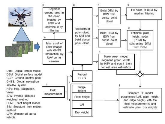
2. Materials and Methods

2.1. Crop and Cultivation Conditions

Materials Sweet potatoes are widely grown all over the world because they grow on poor land. The tuberous root of sweet potatoes provides a rich source of starch and dietary fiber. Leaves are also consumed as vegetables in some areas. It was brought to Japan around the early 17th century. Currently, it is widely cultivated all over Japan [34].
In this study, a 60 × 20 m sweet potato field, located in Ecosystem Research Field II (36.0508 °N, 140.075 °E) of the National Institute for Environmental Studies in Tsukuba, Ibaraki, Japan, was used. Sweet potato (Ipomoea batatas L.) cv. Beniazuma, which is the most widely grown cultivar in Ibaraki, Japan, was used. The sweet potatoes were grown in multi-cultivation, and the ridges were covered with black vinyl sheets. The average height of the ridges was about 21 cm. The field of 60 m × 20 m was divided into six blocks (S1 to S6) of 10 m × 20 m.
Different amounts of fertilizer were applied for each block. The amounts of fertilizer used in each block varied between 0, 0.025, 0.02, 0.1, 0.15, and 0.2 kg/m2. The standard amount of fertilizer commonly used is 0.15 kg/m2 (Figure 2a). A commercial fertilizer that contains 3% nitrogen, 10% phosphoric acid, 10% potassium (Kinsei Kasei No. 3, Taki Chemical Co., LTD., Hyogo, Japan), and a fertilizer of 2% granulated magnesium lime (Tagen Lime Industry Co., LTD., Tochigi, Japan) was applied. Seedlings were transplanted on 27 May 2015 (0 days after planting, or DAP).

2.2. Instrumentation and Measurement Methods

A small UAV, Spreading Wings S1000 (DJI, Shenzhen, China) equipped with a custom made 3-axis gimbal, was used in this study (Figure 1). The deployed diagonal wheelbase size of the S1000 is 1045 millimeters (mm) but can be 650 mm when stored, which is convenient for mobile uses. The standard landing gear length of the S1000 is 305 mm, but for this study it was extended by about 200 mm. This length increases the stability of the take-off and landing of the UAV and allows for the attachment of multiple cameras to the gimbal. Further, to secure proper measurement, S1000 can automatically open and close the landing gears. The maximum power output of the propeller motor is 500 watts (W). The total weight of the main unit is 4.5 kg, and two units of batteries (6S LiPo 8000 mAh) are 6.6 kg. The takeoff weight is 11 kg, and the payload is 4.4 kg. According to the specifications, the flight time was up to 15 minutes, but the practical flight time was about 10 minutes. Flight control was performed by the A2 multi-rotor stabilization controller based on information from the Global Navigation Satellite System (GNSS) and the Inertial Measurement Unit (IMU). Once a flight plan is created on a PC and uploaded to the UAV, it will automatically fly based on the previously configured flight path. The 3-axis gimbal for a camera can be operated in any direction. The gimbal has its own IMU and it can be controlled independently from S1000. This prevents blurring caused by the camera shaking from wind or vibration.
A digital single-lens reflex camera (EOS kiss X7, Canon INC., Tokyo, Japan) was used to measure images. The effective pixels are about 18 million pixels and the weight is about 370 grams (g). Continuous shooting at up to four frames per second is possible; but in this experiment, it was set to an interval of one shot per second. The GNSS coordinate update rate was set to once per second, and the trajectory of the camera movement was recorded using a GNSS receiver GP-E2 (Canon INC., Tokyo, Japan). In order to reduce the influence of wind and vibration, the shutter speed priority program mode was selected, and the shutter speed was set to 1/1000 seconds and the diaphragm was automatically adjusted. The measurements for each period used the same flight route. To improve the accuracy of the 3D model, fourteen iron columns with a height of 30 cm and a diameter of 5 cm with yellow marks at the top were installed as Ground control points (GCPs) at the boundaries of each block around the sweet potato field (Figure 2, shown as red colored circle marks). The GNSS coordinates of each GCP were recorded using a GNSS receiver GP-E2 (Figure 1j). UAV measurements were made at an altitude of approximately 30 m above the ground, from 11:00 to 14:00, when the sun’s altitude was sufficiently high. Measurement dates were five days and the dates were 10 June (14 DAP), 29 June (33 DAP), 10 August (75 DAP), 5 September (101 DAP), and 15 October 2015 (141 DAP). The measurement for each period was performed using a 28 mm focal length lens, except for 10 June, 10 August, and 15 October. During these three days, data taken by a 50 mm lens were added and compared with images captured by a 28 mm lens. The survey of the ground surface was conducted on the same day as the UAV measurement. Ridge heights and plant heights on the site were measured with a ruler, by selecting ten places in each fertilizer block on each measurement date. In addition, 1 m × 1 m sample areas were established for each fertilizer block, and LAIs and dry weights of the above-ground parts were determined by cutting plants. The minimum measurement unit of the ruler was 1 mm. Collected sample leaves were placed on a flat desk and the LAI was determined by processing images taken by a camera. The dry weight of the above-ground parts was measured by drying at 80 ℃ for one day. The tuberous roots collected on 15 October of the harvest day were finely sliced and dried at 80 ℃ for two days, and then the dry weight was measured (Figure 1k).

2.3. Development and Accuracy Evaluation of Ground Surface Model and Plant Height Model in Ridge Cultivation

Figure 1 shows a workflow of the construction of the ground surface model and the plant height model in ridge cultivation. First, at different growth stages, the sweet potato field was continuously measured with a camera mounted on a UAV to obtain 2D color images with GNSS coordinates (Figure 1a). Next, in order to construct 3D Digital Surface Models (DSMs) including plants and ground surfaces, 3D point cloud models with color information were constructed from the acquired images using the SfM. Then, the data were converted into 3D dense point cloud models with color information (Figure 1c).
The series of calculations were computed using Agisoft Photoscan (Agisoft LLC, St. Petersburg, Russia), which is commercially available. The following procedures were used for the generation of 3D point cloud models. First, by using the Scale-Invariant Feature Transform (SIFT) method, multiple key points of 2D images were searched repeatedly [35,36]. Then, the 3D coordinates of the obtained key points were calculated [37]. Errors were minimized using the Bundle-Adjustment method [38]. Noises were removed using the Clustering Views for Multi-View Stereo (CMVS) method, and then the 3D dense point cloud models were created [39,40]. Since 2D images acquired by the camera have coordinate information such as longitude, latitude, and altitude, this information was used for the calculation. Also, 3D point cloud models were aligned using GCPs which were installed on the ground (Figure 1j). The 3D dense point cloud models were generated by increasing the accuracy of the point cloud models through the correction calculation (Figure 1c). Conversion of the 3D dense cloud models into 3D DSMs was conducted using the inverse distance weighting (IDW) method, which interpolates and fills in the missing images [31].
Following the estimation method of the 3D ground surface model (Digital Terrain Model, DTM), a series of 2D color images capturing sweet potato vegetation was used. A series of 2D color images with GNSS data (which was captured on 10 June with relatively low plant coverage) were used (Figure 1a). In the Hue, Saturation, Value (HSV) color model, H values between 70 to 150 and V values 20 or more are categorized as vegetated areas, and then a binary image was generated, which indicates the vegetated area as white and the non-vegetated area as black (Figure 1b). A previously used method was employed in this study [41]. It is common to utilize the HSV color system to remove the green component, since it is difficult to remove the color using RGB color system. In order to remove the influence of the shadow around the plant, enlargement filter processing ranging from 1 × 1 pixel to 15 × 15 pixels for the vegetated area (white part) was used (Figure 1b). Enlargement filtering is to enhance white pixels around a single white pixel. This was conducted to remove the shadows around the plant. This process was programmed using IDL 8.0 (Harris Geospatial Solutions, Inc., Tokyo, Japan). For the mask processing, a binary image created with the previous process was applied for the original color 2D image. The process was performed using Agisoft Photoscan. The method described in an Agisoft manual was used [42]. The 3D point cloud model was created using the SfM, and then the 3D dense point cloud model was generated (Figure 1c). The DTM was calculated using the IDW method with the 3D dense cloud point model (Figure 1d). However, with the DTM obtained under this process, part of the plants and shadows remained as holes in the image. In order to fill in the holes and obtain an accurate 3D DTM with ridge shape information, rectangular median filter (N × M pixel, N = 1 to 37, M = 1 to 5) processes were applied (Figure 1e). The long side direction of the filter was determined based on the direction of the ridges. The maximum and the minimum heights of a ridge were determined based on the derived DTM, and heights of the ridge were calculated. The 3D Plant Height Models (PHMs) were generated by subtracting the DTM of 10 June from the DSMs constructed from the image set at each measurement time (10 June, 29 June, 10 August, 5 September, and 15 October). Using the PHM determined, the highest points of individual plants at each measurement time were extracted, and the plant height was determined (Figure 1g). During the experiment periods, actual plant heights of ten consecutive plants in each ridge in different blocks were measured, and also location information of the plants measured was recorded. The highest PHM was measured using ENVI (Esri Japan, Tokyo, Japan) and location information was referenced. The error evaluation was performed by comparing the plant height and ridge height estimated from the models with the actual measured values (Figure 1l).

2.4. Estimation Method of LAI and Dry Matter Weight and Their Accuracy Evaluations

LAI was estimated by a regression model because the vegetative leaf overlapping was significant. It is also difficult to measure the LAI directly because of this overlapping. To obtain LAI estimation, a 3D dense point cloud model with color information (Figure 1c) was converted into a 3D voxel model with color information of 1 cm × 1 cm × 1 cm. The size was determined based on the resolution of 2D images, which was approximately 1 cm × 1 cm. IDL 8.0 software (Harris Geospatial Solutions, Inc., Tokyo, Japan) was used to calculate voxels. For voxel calculation, green points were extracted from dense points cloud data, and the points within the region of interest (ROI) were converted into voxels with the coordinate system of X, Y, and Z axes. The region without any vegetation was treated as a null voxel. The data of the dense point cloud has different or, non-uniform, point density and position coordinates. Therefore, it is not adequate to use such point cloud data to estimate area data. For this reason, after converting dense point cloud data into georeferenced voxel data, the correlation with the area was calculated.
A 1 cm × 1 cm × 1 cm size of the voxel was employed in this study. This is a nice round number often used for UAV based SfM analysis. However, the resolution was slightly smaller than the resolution of PHM, which was derived by the dense point cloud data. Nevertheless, rather than using the dense point cloud data directly, we considered that the utilization of georeferenced data is appropriate to calculate the correlation with the leaf area data. The plant areas (70 < H < 150 and V > 20) were extracted using the HSV color model, and the number of voxels were counted based on a previous publication [41]. Usually, the HSV color system is used to remove green components, since it is difficult to remove green colors using the RGB color system. Then, the regression equation for the LAI was obtained from the voxel count and the actual measurement was determined. The equation was used to determine the correlation and estimation of the LAI (Figure 1h). An accuracy comparison was also performed between the estimation equation obtained from the previous process and the estimation equation obtained by extracting a plant region from a 2D image. Lastly, the correlation between the estimated LAI and the dry weight and yield of the above-ground parts was determined. Then, the estimation equations were calculated (Figure 1l).

3. Results

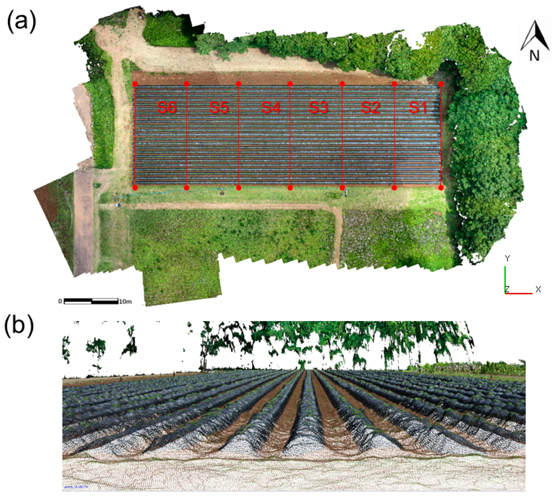
3.1. Examples of 3D Dense Point Cloud Models of the Sweet Potato Field

Figure 2 shows examples of the top view (a) and side view (b) images of the 3D dense point cloud model with color information for the sweet potato field on 29 June, or 33 DAP. The measurement was made by a UAV from about a 30 m height, with a camera equipped with a 28 mm focal length lens. The effective pixels are about 18 million pixels, and an approximate resolution size was 1 cm × 1 cm. A 3D dense point cloud model was generated from the series of 2D color images obtained with GNSS coordinate data. Sizes of sparse models are from 2,582,260 to 5,902,547 points for 28 mm lens-based data and 2,665,378 to 3,122,074 points for 50 mm lens-based data. Further, sizes of dense cloud models were from 2,516,8884 25,168,884 to 28,818,086 points for 28 mm lens-based data and 34,976,385 to 44,298,887 points for 50 mm lens-based data. The number of points were counted using the Agisoft PhotoScan. The spatial resolutions of 3D models were 1.6 to 1.8 cm/pixel for 28 mm lens-based data and 0.9 to 1.1 cm/pixel for 50 mm lens-based data. The resolution slightly varied each measurement. The maximum average number of voxels was 4514 voxels/m2 for 28 mm lens derived data. Data on 50 mm lens derived data are not available, since the data were not used for voxel construction. The number of voxels was counted using IDL 8.0 (Harris Geospatial Solutions, Inc., Tokyo, Japan).
The red lines in Figure 2a indicate the boundaries of each fertilization block. From the right to the left, S1 is the 0 kg/m2 fertilization block followed by 0.025 (S2), 0.02 (S3), 0.1 (S4), 0.15 (S5), and 0.2 kg/m2 (S6). Red colored circles at both ends of the red line are positions of GCPs (iron columns with 30 cm in height and a diameter of 5 cm with yellow marks at the top). The sweet potato field was surrounded by roads, and trees were abundant in the northeast border. In the field, the ridge was covered with black vinyl sheets for multi-cultivation, and ridges were lined up in the east-west direction. The entire image of the field can be seen from the top view image in Figure 2a. Further, characteristics of the ridges and the sweet potato leaves are evident from the side view image in Figure 2b. At this stage, because the plants have limited growth and are not very leafy, it is easy to perceive the separate plants, ground, and black vinyl sheets. Since distant trees could not be measured, some side portions of the trees are missing from the 3D constructed image. Although not shown here, as the plant leaves grew, the ground surfaces were covered by plants, and by 10 August, all parts of the field were covered with plants. The dark dead leaves increased around 5 September, and the yellow dead leaves became noticeable around 15 October.

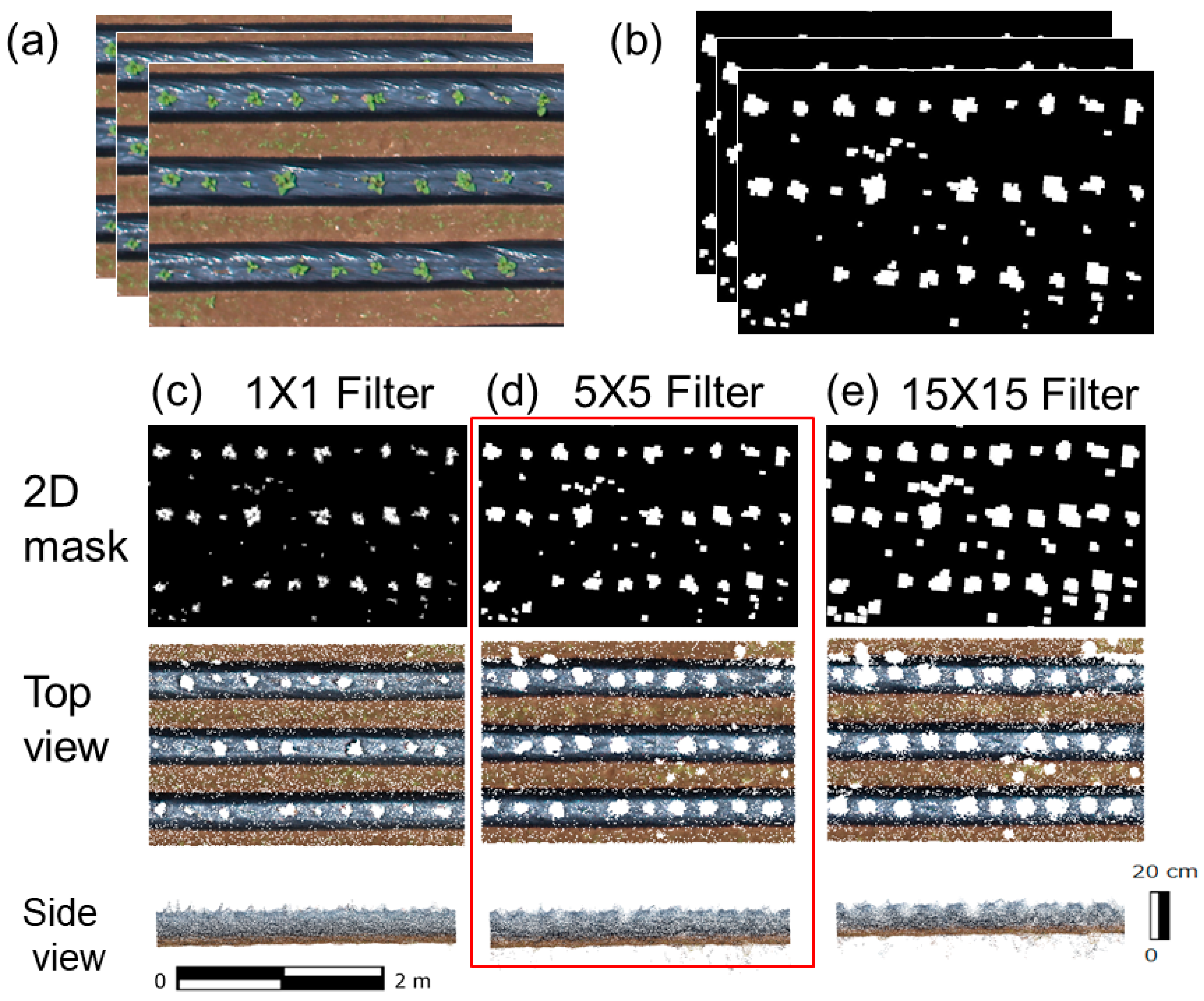
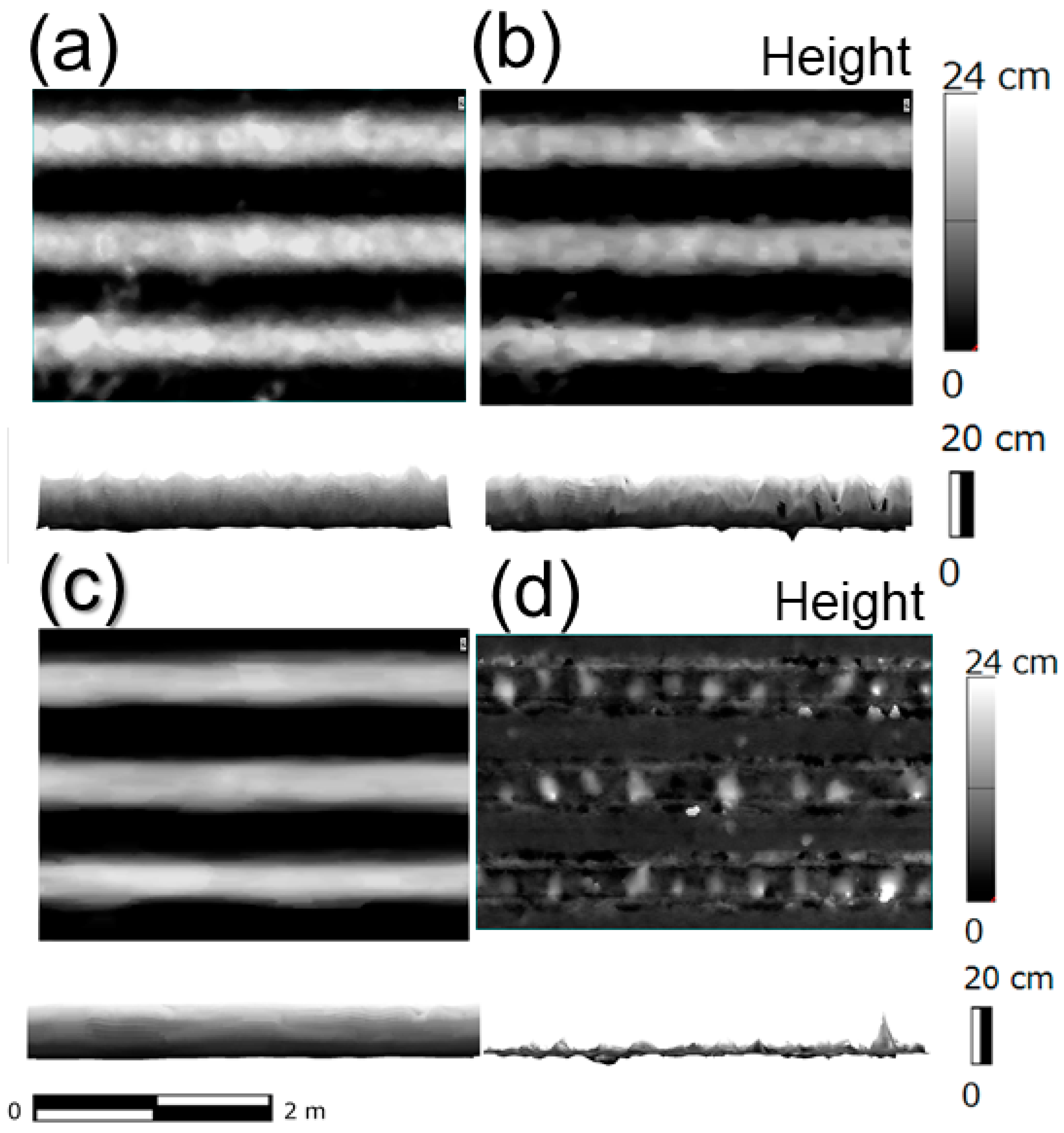
3.2. Effects of Plant Area Removal and Filtering Process for the Construction of Ground Surface (DTM)

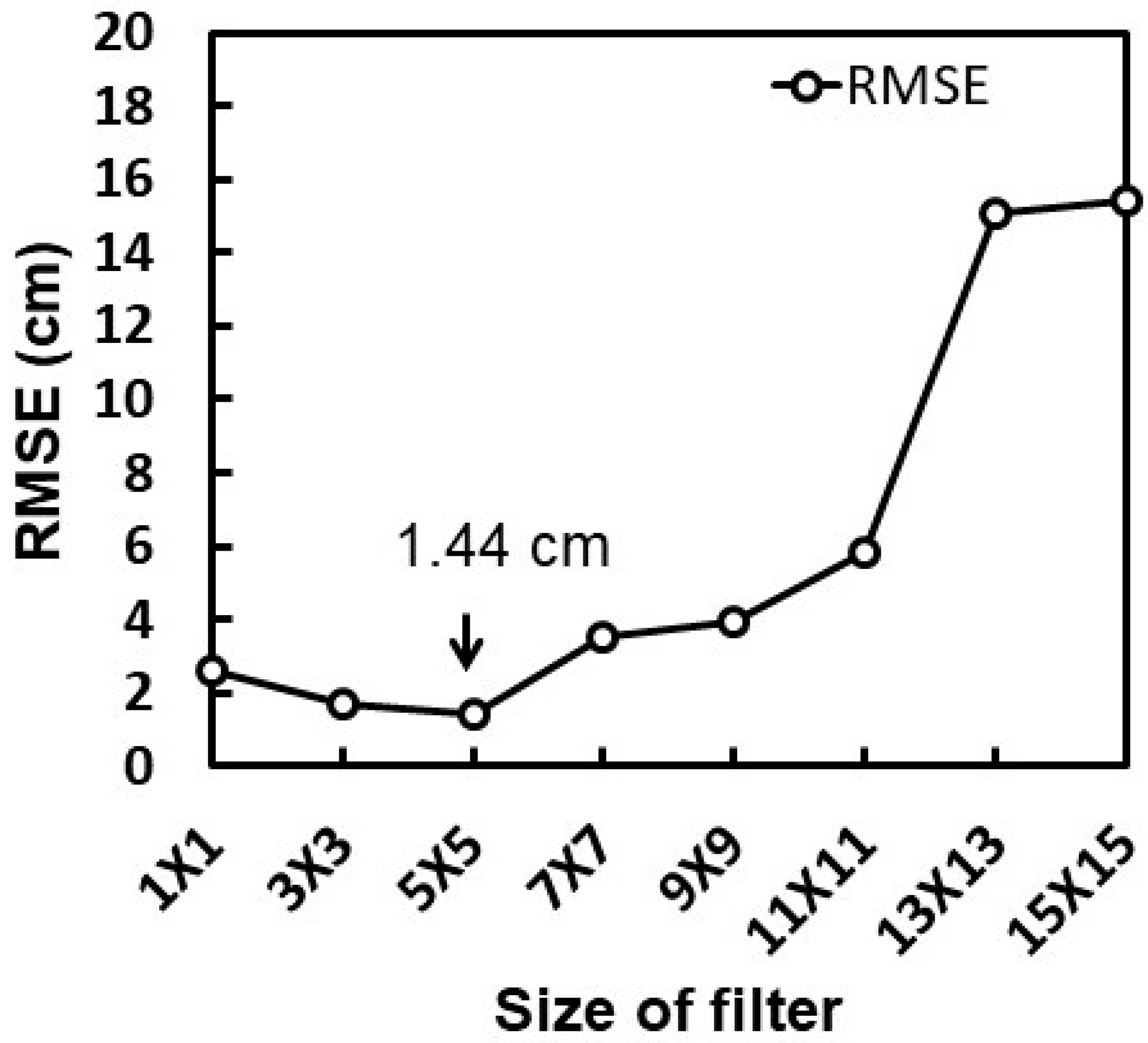
3.2.1. Effects of Plant Area Removal and Enlargement Filtering

Two-dimensional color image data measured on 10 June were used to generate ground surface (DTM) data, because the data had relatively low plant coverage. Figure 3 shows examples of plant area removal and enlargement filtering (Figure 1b) to construct the ground surface (DTM) data. Dark brown soil and black vinyl sheets were observed in the 2D color image shown in Figure 3a. The 2D color image of Figure 3a was based on threshold values using the HSV color model as described in method 2.3.
A binary image was created based on the vegetated area (white) and non-vegetated area (black) (Figure 3b). Three-dimensional dense point cloud models (Figure 3c–e) were constructed using SfM with the images. Binary images are shown on the top of this figure, the top views of the 3D dense point cloud models are shown in the middle, and images of the side views are shown at the bottom of the figure. Uneven shapes can be seen in the side view image of Figure 3c. This is due to the thresholding process mentioned above with the effects of shadows around plants.
Therefore, the enlargement filter processing was performed for the vegetated areas (white part) to remove the shadows around the plant. Figure 3c is an example of 1 × 1 filtering, Figure 3d is an example of 5 × 5 filtering, and Figure 3e is an example of 15 × 15 filtering.
Figure 4 shows an error comparison between the actual value and the estimated value of the ridge heights obtained from the DTM, which was processed with different sizes of enlargement filters. Note, that in the DTM constructed, the hole caused by the removal of the vegetated area remains. Therefore, an error evaluation of the estimated and actual value of places other than holes was performed. When using the 5 × 5 filter, the error of the ridge height was minimized, and the Root Mean Square Error (RMSE) was 1.44 cm. Filter sizes of less than 5 × 5 did not work well to remove the shadow area around the plants. In the case of filter sizes larger than 5 × 5, the error became large due to the loss of the ground surface accompanying the expansion of the hole.

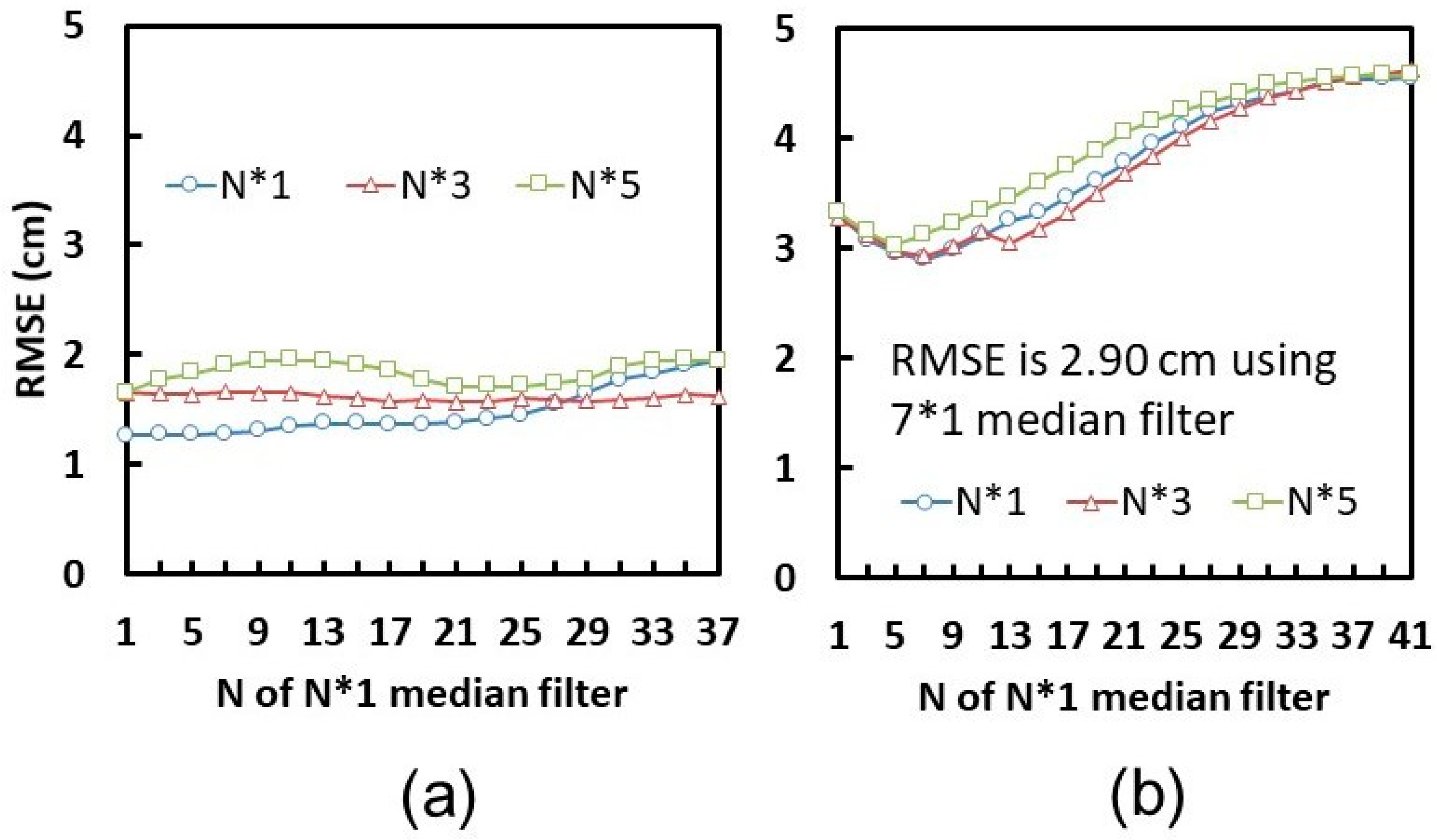
3.2.2. Effects of Median Filters

The enlargement filtering of the plant area alone leaves holes when constructing the ground surface (DTM). In order to fill such holes, median filters with rectangular N × M, where N is the number of pixels in the direction of the ridge, and M is the number of pixels in the cross-sectional direction of the ridge, were tested. Figure 5a shows an example of a DSM including the plant and the ground surface, which was measured on 10 June (Figure 1f).
Figure 5b shows an example of DTM after 5 × 5 enlargement filter processing, which is shown in Figure 3D. The entire process is shown in Figure 1d. Note that top view images are shown in the upper part, and side view images are shown in the lower part. In Figure 5b, while plants and shadows are completely removed, large holes can be seen in DTMs because of the removal of the plant area and the enlargement filtering process. Figure 5c shows the result of median filtering to fill the holes. Although, median filtering was performed with N = 7 and M = 1, the unevenness of the ground surface could be reduced while leaving the shape of the ridges. Figure 5d is a plant height model (PHM) obtained by subtracting the DTM (Figure 5c) from the DSM (Figure 5a).
Figure 6 shows the errors between the estimated values and the actual measurements of ridge heights (DTM) and plant heights (PHM) due to the difference in size of the N × M median filters applied to the DTM. In these cases, where there is an error in the ride heights (A), the smaller the filter size, the smaller the error. This is because the error evaluation was made without the hole portions. The RMSE was 1.44 cm with a filter size of N = 1 and M = 1. On the other hand, the error of the plant height was the smallest with a filter size of N = 7 and M = 1, with an RMSE of 2.90 cm. This is because the filter size N in the direction of the ridges needs to be a size that would fill the hole, but if it is too large, the shape of the ridges will differ from the actual shapes. For the filter size M, a smaller filter size worked better. Filter size M is defined for the cross-sectional direction of the ridge. The cross-sectional direction of the ridges should have the smallest size, which does not affect the shape rather than the filling effect.

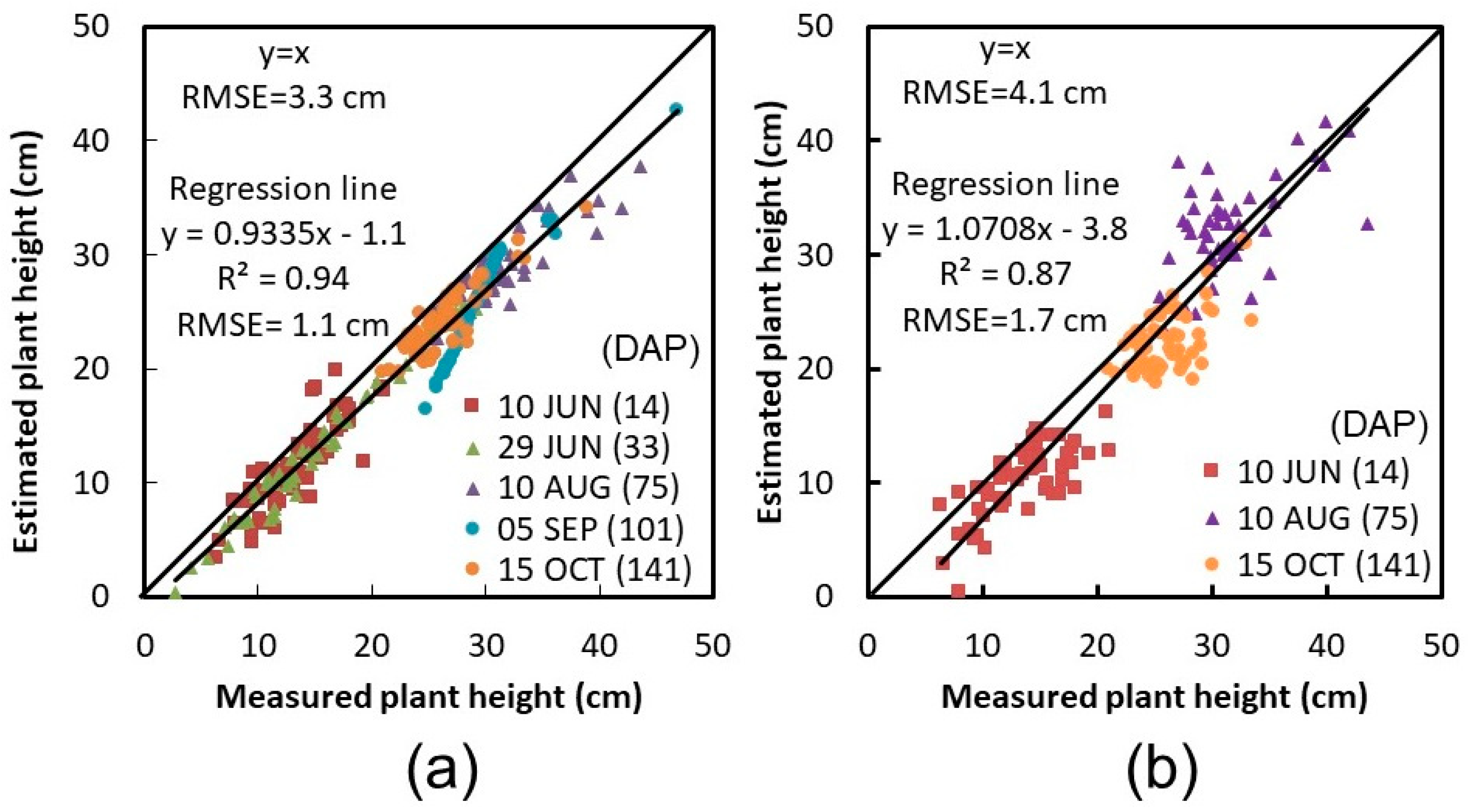
3.3. Error Evaluations of Plant Height Models (PHMs) over the Entire Growth Period

In the previous section, errors between the actual measurements and the estimated values from the plant height model (PHM) derived from 10 June data was described. In this section, the error evaluations of PHMs were performed over the entire growth period (10 June, 29 June, 10 August, 5 September, and 15 September) from the planting of seedlings to the harvest time. PHMs were generated by subtracting the DTM of 10 June from the DSMs of each growing period. Figure 7 shows the measured values versus the estimated values. Figure 7a shows a comparison of the actual measured values versus the PHM constructed values from an image set measured with a 28 mm focal length lens, and Figure 7b shows the result obtained using a 50 mm focal length lens. Approximately 300 points were compared for the 28 mm lens generated data, and about 180 points were compared for the 50 mm lens generated data. In the figures, the horizontal axis (x) shows the actual measurement values, and the vertical axis (y) shows the estimated values from the PHM.
In the case of a lens with a 28 mm focal length, the error with y = x had an RMSE of 3.3 cm, the determination coefficient of the regression equation (y = 0.9335x − 1.1) was R2 = 0.94, and the error with the regression equation had an RMSE of 1.1 cm. When a lens with a 50 mm focal length was used, the error with y = x had an RMSE of 4.1 cm. The determination coefficient of the regression equation (y = 1.0708x − 3.8) was R2 = 0.87, and the error with the regression equation had an RMSE of 1.7 cm, which was larger than the RMSE obtained with a 28 mm focal length lens. The estimated values tended to be slightly lower than the actual values in both lenses. Despite the use of the 10 June DTM, the changes in errors over the entire growth period were relatively small, which indicates that generation of a PHM with high accuracy is possible. Slightly larger errors have been derived from the data measured with a 50 mm focal length lens. This is because the overlap rate of 2D color images was poor due to the UAV’s altitude and flight speed. This may have caused errors when the 3D models were generated by the SfM.

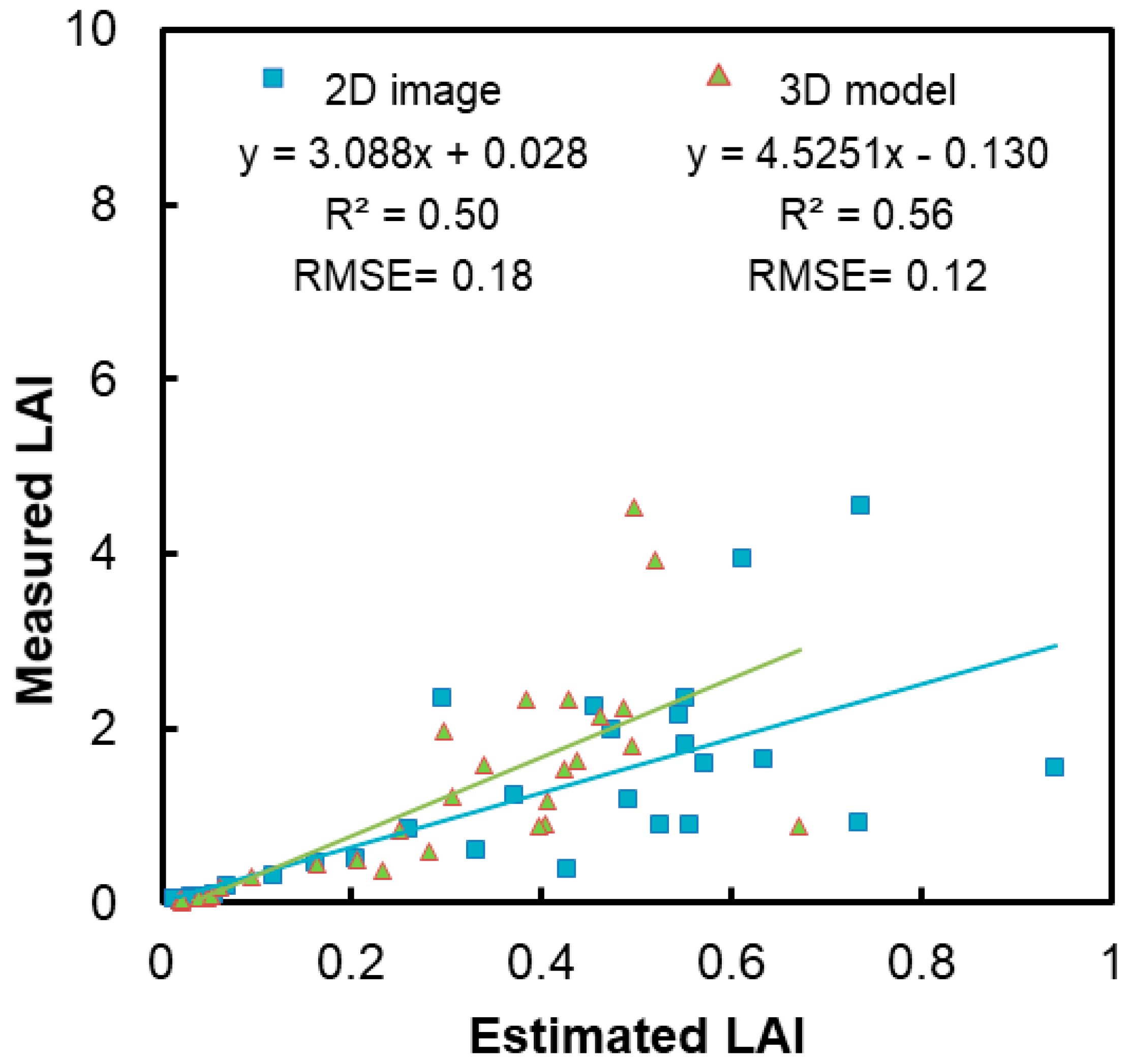
3.4. Estimation of LAI and Error Evaluation

Figure 8 shows the estimated LAI values (x) versus the actual measurement values (y). The estimated LAI values were obtained by counting the number of voxels of the 3D voxel models. The 3D voxel models from each sample area at each growth stage were used. The 3D voxel models used were generated from the image of a 28 mm lens, which obtained satisfactory results in PHMs. Figure 8 also shows the estimated LAI derived from counting the number of plant area pixels in 2D images. The estimated values always underestimated the LAI in both the 2D image and the 3D voxel model. In fact, the ratio of the estimated value to the actual measured value was 1/10, when the leaf area was largest with the LAI of 4.5. This indicates that it is difficult to measure the lower leaves when plants are fully grown, from the aerial images of a UAV, regardless of the 2D or the 3D data. However, the determination coefficient R2 = 0.56 (RMSE = 1237.3 cm2/m2) of the regression equation (y = 4.5251x − 1299.3) determined from the 3D voxel model is better than the determination coefficient R2 = 0.50 (RMSE = 1825.0 cm2/m2), which was calculated by the regression equation (y = 3.0880x + 276.5) determined from the 2D image. Moreover, errors were smaller for the 3D voxel model. This is thought to be due to the fact that the 3D voxel model loses slightly less of the 3D structure of the leaves than the 2D image.

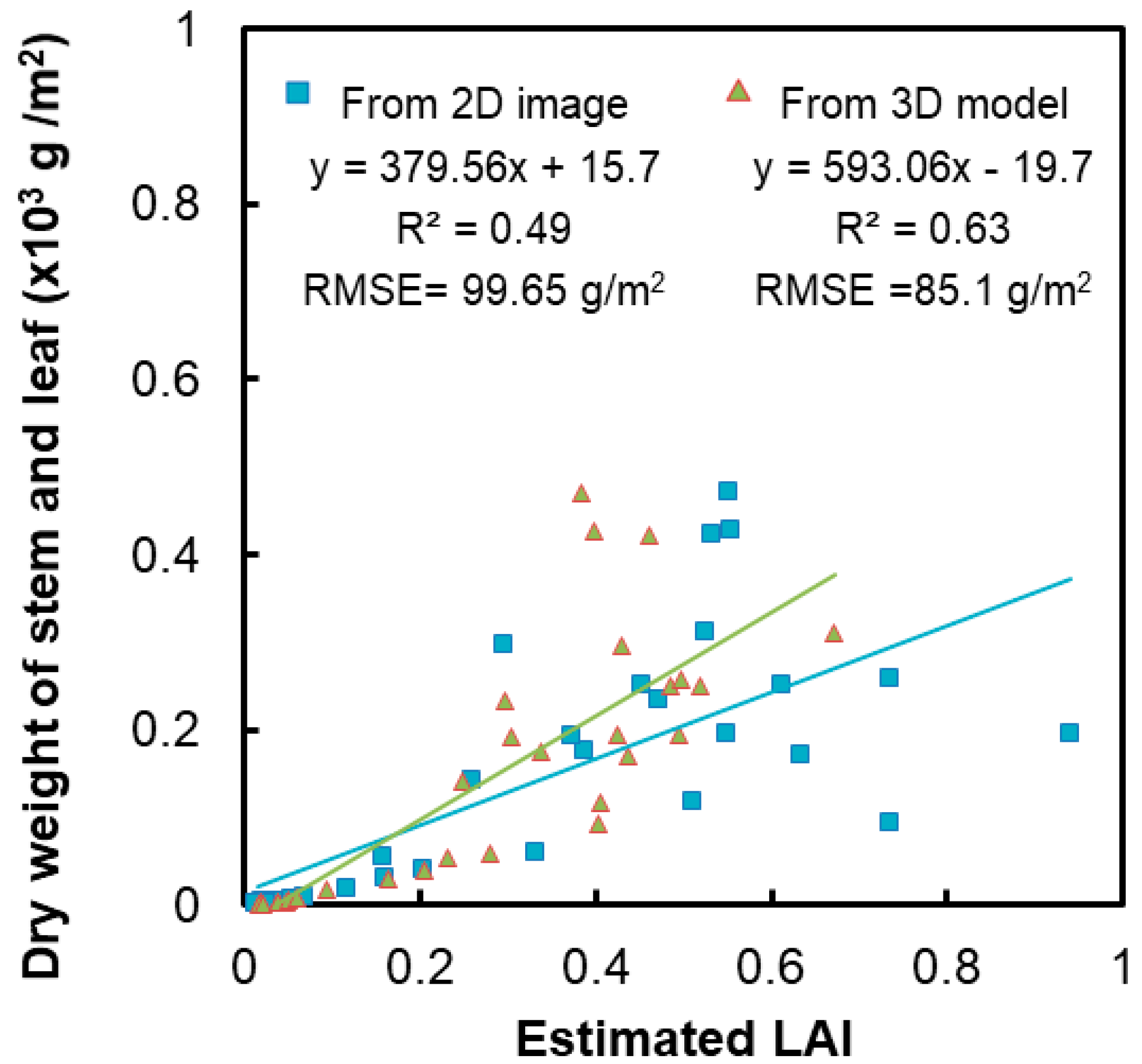
3.5. Relationships Between LAI and Aboveground Dry Matter Weight, and Tuberous Root Yield

Figure 9 shows the relationship between the LAI estimated from the 3D voxel model and the above-ground dry matter weight (stem and leaf). The relationship between the LAI estimated from the 2D image and the above-ground dry matter is also shown in Figure 9. The relationship between the LAI (x) and dry matter weight (y) obtained from the 3D voxel model was y = 0.0593x − 19.7 (R2 = 0.63, RMSE = 86.1 g/m2). Similarly, y = 0.0380x + 15.7 (R2 = 0.49, RMSE = 99.6 g/m2) was obtained using the 2D image data. The 3D voxel model showed a better coefficient of determination and a smaller error.
Table 1 shows the relationship between the estimated LAI using 2D images of each growth period and the dry matter weight of tuberous roots harvested on 15 October.
Similarly, Table 2 shows the relationship between the estimated LAI using 3D voxel models and dry matter weight of tuberous roots.
Regardless of the 2D image or the 3D voxel model-based estimations, the best determination coefficient R2 and the minimum RMSE were obtained from the data derived on 29 June. Also, by comparison, better results were obtained from the 3D voxel model than the 2D image. In the case of the data derived from 29 June, the 3D voxel model showed R2 = 0.69, and RMSE = 125.7 g/m2, while the 2D image showed R2 = 0.55, RMSE = 152.0 g/m2. This is thought to be due to the fact that the estimation accuracy of the LAI is reduced when the plants are fully grown, and, as a result, the accuracy of the yield prediction is decreased. This result showed that a relatively accurate estimation of the tuberous root yield y (g/m2) can be made based on the regression equation of y = 0.2281x + 51.5 from the LAI x (cm2/m2) obtained from the 3D voxel model on 29 June at the early growth stage.

4. Discussion

In this research, the SfM method, a passive method to construct a 3D model from a series of 2D color images taken with a consumer grade single-lens reflex camera mounted on a UAV, was utilized to generate 3D models of ground surfaces and plant communities. Sweet potato fields cultivated on a ridge (after planting the seedlings) were used for this study. Further, methods to estimate changes in growth parameters, such as plant height, LAI, biomass, and tuberous root yield, were examined. Errors of such parameters were also evaluated. In general, in agricultural fields, the ground surface is not always flat, as in the case of ridge cultivation. It is often difficult to observe the ground surface before plant growth because crop cultivation would be started right after shaping the ridges.
For this reason, first, the removal processes of plant areas and their shadow areas using the HSV color model were examined at the early stages of growth. Then, construction of a 3D ground surface model (DTM) with high accuracy was examined. When only the plant area was removed, then the data obtained had significant errors. In addition to the holes created by the removal of the plants, uneven shapes remained that were considered to be effects of shadows. Therefore, in order to remove the influence of such shadows, enlargement filter processes from 1 × 1 pixels to 15 × 15 pixels were performed to enlarge the holes from the shadows of the plant area in the 2D color images (Figure 3). As a result, the 5 × 5 enlargement filter was the most effective, and its expansion width was about 2.5 cm. The results showed that it is important to remove the shadow effect and to use an appropriately sized hole enlargement filter that will not affect the unevenness of the ridges. Then, it is necessary to fill the holes created by the process mentioned above. However, in order to build an accurate DTM of rough surfaces such as ridges, it is necessary to use a special hole-filling filter. In this study, rectangular median filters, which have a larger size in the direction of the ridge (N × M), were used. The result showed that the error is the smallest at a filter size of N = 7 and M = 1. The error in plant height had an RMSE of 2.90 cm. This means that the filter size N in the ridge direction needs to be a size that fills the hole (approximately 7 cm). If the size of the filter is too large, the shape of the ridges will differ from the actual shape. Therefore, it has been found that the cross-sectional direction of the ridges should be of the smallest size, which does not affect the shape rather than the filling effect. When the error evaluation for holes was performed, since holes could not be measured, RMSE was approximately 1.44 cm. In terms of the error factor for plant height, the error was large with an RMSE of 3.3 cm, and there was a tendency to underestimate. This is thought to be because the sharp unevenness on the top of the plant height model cannot be sufficiently reproduced. In addition, there was a ground surface RMSE estimation of about 1.44 cm. Therefore, the tip of the plants was removed from the model, which caused an underestimation in plant height. Plant heights derived from a 28 mm focal length lens showed a 0.8 cm better RMSE result, while plant heights derived from a 50 mm focal length lens showed an RMSE of 4.1 cm. Theoretically, a higher accuracy can be expected with the 50 mm lens, since the spatial resolution of the 50 mm lens is about 0.5 cm, while that of the 28 mm lens is about 0.8 cm. The SfM usually requires an overlap of nine or more images. Since the angular field of view of a 50 mm lens was smaller, only an insufficient number of overlapped images could be obtained in this measurement. The number of overlapped images necessary is determined by the angular field of view, the shooting interval, flight altitude, flight path, flight speed, and the shooting time, among other conditions. Therefore, it is important to take measurements considering such parameters, as well as the processing time of the SfM.
Although the methods used were different from the procedure studied in this research, there have been some reports on the construction of 3D DSMs with plants and ground surfaces, and ground surface DTMs based on the 3D dense point cloud models derived by UAV-SfM. Further, the plant height models, or PHMs, have been discussed, and the accuracy of such PHMs has been examined.
For the forest research, Dandois and Ellis [20] conducted research on mixed forests (which were dominated by American beech, oak, and hickory) and other types of forests. The plant height observed in their study varied from approximately 9 to 43 m. Noise reduction was applied to the point cloud models using the rectangular median filter. Then, DSM and DTM were estimated, which resulted in RMSEs of plant height estimation from 390 to 1090 cm.
Diaz-Varela et al. [19] conducted a study on olive trees with canopy heights of 2 to approximately 3.5 m. They reported errors in estimation of plant heights in RMSE from 10 to 45 cm. In this study a circular region of 2 m was used to calculate the ground reference height as minimum DSM values. Teng et al. [32] studied Japanese Larch trees with plant heights between 12 to 14 m. They reported that when DSMs and DTMs are constructed by using the IDW method for 3D dense point cloud models, the error estimation is an RMSE of 47 cm.
For field crops, Holman et al. [21] studied wheat with crop heights between 0.5 to 1.2 m. Crop heights were calculated by subtracting the Digital Elevation Model (DEM) from the DSM. Then, they concluded that an RMSE of 7.0 cm or better can be expected for crop height estimation.
Research on trees and crops have been conducted on relatively flat ground surfaces. However, some crops can be grown using uneven ground surfaces, such as with ridge cultivation. It takes a relatively short time from shaping ridges to planting. Therefore, it is necessary to generate the DTM with uneven ground surfaces while crops are being cultivated. Kim et al. [22] conducted research on Chinese cabbage and white radish with crop heights of 0.05 to 0.45 m under ridge cultivation. By using DTMs that were generated before the cultivation and DSMs during the cultivation, plant heights were evaluated. The authors reported the coefficient of determination (R2) of the regression lines based on the actual values and estimated plant heights. The coefficient of determinations (R2) was 0.95 for Chinese cabbage and 0.91 for white radish. However, they did not provide the RMSE of the plant height. further, they did not discuss the accuracy estimation of the ridge height.
In this research, using sweet potatoes in ridge cultivation, a method was developed to generate the DTM with an RMSE of approximately 1.44 cm for the uneven ground surfaces at the early growing stage. Further, accurate plant heights can be estimated, with an RMSE of 3.3 cm for the entire cultivation period with plant heights between 0.03 to 0.45 m.
Even though the DTM was constructed from point cloud data during the cultivation period, and the DTM was created for ridge cultivation with uneven surfaces, highly accurate DTM and PHM was able to be generated in comparison to the previous research.
There are only a few studies that focus on the accuracy assessment of leaf area and biomass estimation using 3D dense point cloud models derived by UAV-SfM. Mathews & Jensen [23] conducted research on the LAI estimation of a vineyard. They used a vineyard with an observed LAI between 0.5 to 5.5. Point extractions were made using rectangles sized 1 m × 2 m, centered on sample vine trunk locations. Then, point cloud heights between 0.3 m and 2.3 m were used for the calculation. Subsequently, the regression line was based on the actual values, and the estimated values of the leaf area were calculated. The results showed that the estimation of errors for LAI were an R2 of 0.57 and an RMSE of 0.236.
Sweet potato cultivation with a LAI between 0.1 to 4.5 was used in this study. Vegetated areas were extracted by color index. Further, the data were converted into the voxel model of 1 cm × 1 cm × 1 cm, and the number of voxels in the plant area was counted. The results showed an R2 of 0.56 and an RMSE of 0.123. These results are comparable with the results of Mathews and Jensen [23].
Regarding the above-ground biomass, Bendig et al. [30] conducted a research on summer barley when the above-ground dry biomass was 30–2700 g/m2. Plant height crop surface models (CSMs) were constructed from point cloud models. Then regression models were used to estimate the dry biomass. Regression models were calculated using the estimated and observed dry biomass. As a result, the estimation errors of above-ground dry biomass were an R2 of 0.39 to 0.68, and an RMSE of 420 to 830 g/m2.
Further, Kim et al. [22] estimated the above-ground biomass (fresh weight) using PHMs. The PHMs were calculated to subtract the DTM before planting from the DSM. Then, the regression equation between the PHM and the measured values was obtained. The models were constructed when the above-ground biomass (fresh weight) of white radish and Chinese cabbage was 0 to 530 g/m2 and 0 to 1300 g/m2, respectively. They reported that R2 was 0.83 in white radish, and the R2 of Chinese cabbage was 0.89. However, the RMSE was not reported in the paper.
This kind of study could be useful for the prediction of harvest weight. Potential predications based on the early stage of plant growth might be possible since a better R2 and RMSE was obtained on 33 DAP and 75 DAP. It would be also useful for the optimization of farm management (i.e., the management of nutrients and water) and also the construction of 3D map of farms.
Since there is a relationship between LAI and plant canopy reflectance, this kind of research could be useful for such a study. The measurement of LAIs using UAV-SfM was discussed in this study. Similarly, the measurement of canopy reflectance using UAV has been discussed in Fang et al. (2016). UAV-SfM derived data could provide useful methods to feed data, such as LAI and other plant characteristic data, into canopy reluctance models, and to generate other plant canopy related information.
In our study, when the above-ground biomass (dry matter weight) was 2 to 470 g/m2, the regression equations for the LAIs were derived from the voxel models, and dry matter weight was calculated. Results showed an R2 of 0.63, and an RMSE of 86.1 g/m2.
To date, no research has been reported on the estimation of below ground biomass and yields. In this research, the yield of tuberous roots was estimated by the regression equation for estimated LAI and the actual tuberous root yields. The actual yields (dry matter weight) of tuberous root were 109 to 722 g. The LAI was estimated based on the 3D voxel model derived by the data obtained from 29 June (33 DAP). The accuracies of the estimation were an R2 of 0.69 and an RMSE of 125.7 g/m. Sweet potatoes were grown in the ridge cultivation at an experimental farm. Different amounts of nitrogen fertilization were applied to diversity biomass production, and 3D dense point cloud models were constructed from a series of 2D color images measured by UAV-SfM.

5. Conclusions

In this study, methods to construct 3D models, DSM, DTM, and PHM, were proposed. Although it was in the early stage of cultivation, a complex ground surface model of ridge cultivation with vegetation was generated, and the uneven ground surface could be estimated with an accuracy of 1.4 cm, and the accuracy of the estimated plant height was 3.3 cm.
After extracting point cloud models of sweet potato plants from dense point cloud models using a color index, voxel models were generated. Then, LAIs were estimated using a regression model with an accuracy RMSE of 0.123. Further, regression models to estimate above-ground and below-ground biomass, or tuberous root weights, based on estimated LAI data, were proposed.
Though this method has an issue with computation time, the UAV-SfM is a relatively inexpensive and highly accurate 3D model generation method among remote sensing technologies. In the future, improvements in computer performance can be expected. Further, by using cameras with higher resolution, as well as thermal and hyperspectral cameras, 3D integrated remote sensing technologies could be utilized for smart agriculture.

Author Contributions

P.T. designed and performed the experiments, modeling and wrote the paper, E.O. reviewed and edited the manuscript, Y.Z. supported the experiments, M.A. supported the field experiments, Y.S. and F.H. discussed on the methods and the results, K.O. designed the experiments, discussed the methods and results, and edited the manuscript.

Acknowledgments

We gratefully acknowledge Mr. Yoshio Suzuki and the support staff in the National Institute for Environmental Studies for the experiments.

Conflicts of Interest

The authors declare no conflict of interest.

References

  1. Campbell, G.S.; Norman, J.M. An Introduction to Environmental Biophysics; Springer Science & Business Media: Berlin/Heidelberg, Germany, 2012; ISBN 1461216265. [Google Scholar]
  2. Jones, H.G. Plants and Microclimate: A Quantitative Approach to Environmental Plant Physiology, 3rd ed.; Cambridge University Press: Cambridge, UK, 2013; ISBN 9780521279598. [Google Scholar]
  3. Omasa, K.; Aiga, I. Environmental measurement: Image instrumentation for evaluating pollution effects on plants. In Systems & Control Encyclopedia; Singh, M.G., Ed.; Pergamon Press: Oxford, UK, 1987; pp. 1516–1522. [Google Scholar]
  4. Omasa, K. Image instrumentation methods of plant analysis. In Modern Methods of Plant Analysis. Physical Methods in Plant Sciences; Linskens, H.F., Jackson, J.F., Eds.; Springer-Verlag: Berlin, Germany, 1990; pp. 203–243. [Google Scholar]
  5. Omasa, K. Image sensing and phytobiological information. In CIGR Handbook of Agricultural Engineering Information Technology; Munack, A., Ed.; American Society of Agricultural and Biological Engineers: St. Joseph, MI, USA, 2006; pp. 217–230. [Google Scholar]
  6. Hobbs, R.J.; Mooney, H.A. Remote Sensing of Biosphere Functioning; Springer Science & Business Media: Berlin/Heidelberg, Germany, 2012; Volume 79, ISBN 146123302X. [Google Scholar]
  7. Sellers, P.J.; Rasool, S.I.; Bolle, H.-J. A review of satellite data algorithms for studies of the land surface. Bull. Am. Meteorol. Soc. 2002, 71, 1429–1447. [Google Scholar] [CrossRef]
  8. Omasa, K.; Hosoi, F.; Konishi, A. 3D lidar imaging for detecting and understanding plant responses and canopy structure. J. Exp. Bot. 2007, 58, 881–898. [Google Scholar] [CrossRef] [PubMed]
  9. Whitlock, C.H.; Charlock, T.P.; Staylor, W.F.; Pinker, R.T.; Laszlo, I.; Ohmura, A.; Gilgen, H.; Konzelman, T.; DiPasquale, R.C.; Moats, C.D. First global WCRP shortwave surface radiation budget dataset. Bull. Am. Meteorol. Soc. 1995, 76, 905–922. [Google Scholar] [CrossRef]
  10. Jones, H.G.; Vaughan, R.A. Remote Sensing of Vegetation: Principles, Techniques, and Applications; Oxford University Press: Oxford, UK, 2010; ISBN 0199207798. [Google Scholar]
  11. Omasa, K.; Qiu, G.Y.; Watanuki, K.; Yoshimi, K.; Akiyama, Y. Accurate estimation of forest carbon stocks by 3-D remote sensing of individual trees. Environ. Sci. Technol. 2003, 37, 1198–1201. [Google Scholar] [CrossRef] [PubMed]
  12. Omasa, K.; Akiyma, Y.; Ishigami, Y.; Yoshimi, K. 3-D remote sensing of woody canopy heights using a scanning helicopter-borne lidar system with high spatial resolution. J. Remote Sens. Soc. 2000, 20, 394–406. [Google Scholar]
  13. Morsdorf, F.; Kötz, B.; Meier, E.; Itten, K.I.; Allgöwer, B. Estimation of LAI and fractional cover from small footprint airborne laser scanning data based on gap fraction. Remote Sens. Environ. 2006, 104, 50–61. [Google Scholar] [CrossRef]
  14. Asner, G.P.; Mascaro, J.; Muller-Landau, H.C.; Vieilledent, G.; Vaudry, R.; Rasamoelina, M.; Hall, J.S.; VanBreugel, M. A universal airborne LiDAR approach for tropical forest carbon mapping. Oecologia 2012, 168, 1147–1160. [Google Scholar] [CrossRef] [PubMed]
  15. Lin, Y.; Hyyppä, J.; Jaakkola, A. Mini-UAV-borne LIDAR for fine-scale mapping. IEEE Geosci. Remote Sens. Lett. 2011, 8, 426–430. [Google Scholar] [CrossRef]
  16. Wallace, L.; Lucieer, A.; Watson, C.; Turner, D. Development of a UAV-LiDAR system with application to forest inventory. Remote Sens. 2012, 4, 1519–1543. [Google Scholar] [CrossRef]
  17. Wallace, L.; Lucieer, A.; Malenovský, Z.; Turner, D.; Vopěnka, P. Assessment of forest structure using two UAV techniques: A comparison of airborne laser scanning and structure from motion (SfM) point clouds. Forests 2016, 7, 62. [Google Scholar] [CrossRef]
  18. Sankey, T.; Donager, J.; McVay, J.; Sankey, J.B. UAV lidar and hyperspectral fusion for forest monitoring in the southwestern USA. Remote Sens. Environ. 2017, 195, 30–43. [Google Scholar] [CrossRef]
  19. Díaz-Varela, R.; dela Rosa, R.; León, L.; Zarco-Tejada, P. High-resolution airborne UAV imagery to assess olive tree crown parameters using 3D photo reconstruction: Application in breeding trials. Remote Sens. 2015, 7, 4213–4232. [Google Scholar] [CrossRef]
  20. Dandois, J.P.; Ellis, E.C. High spatial resolution three-dimensional mapping of vegetation spectral dynamics using computer vision. Remote Sens. Environ. 2013, 136, 259–276. [Google Scholar] [CrossRef] [Green Version]
  21. Holman, F.H.; Riche, A.B.; Michalski, A.; Castle, M.; Wooster, M.J.; Hawkesford, M.J. High throughput field phenotyping of wheat plant height and growth rate in field plot trials using UAV based remote sensing. Remote Sens. 2016, 8, 1031. [Google Scholar] [CrossRef]
  22. Kim, D.; Yun, H.S.; Jeong, S.; Kwon, Y.; Kim, S.; Suk, W.; Id, L.; Kim, H. Modeling and testing of growth status for chinese cabbage and white radish with UAV-based RGB Imagery. Remote Sens. 2018, 10, 563. [Google Scholar] [CrossRef]
  23. Mathews, A.J.; Jensen, J.L.R. Visualizing and quantifying vineyard canopy LAI using an unmanned aerial vehicle (UAV) collected high density structure from motion point cloud. Remote Sens. 2013, 5, 2164–2183. [Google Scholar] [CrossRef]
  24. Badura, G.P.; Bachmann, C.M.; Tyler, A.C.; Goldsmith, S.; Eon, R.S.; Lapszynski, C.S. A novel approach for deriving LAI of salt marsh vegetation using structure from motion and multiangular spectra. IEEE J. Sel. Top. Appl. Earth Obs. Remote Sens. 2019, 12, 599–613. [Google Scholar] [CrossRef]
  25. Li, W.; Niu, Z.; Chen, H.; Li, D.; Wu, M.; Zhao, W. Remote estimation of canopy height and aboveground biomass of maize using high-resolution stereo images from a low-cost unmanned aerial vehicle system. Ecol. Indic. 2016, 67, 637–648. [Google Scholar] [CrossRef]
  26. Jensen, J.L.R.; Mathews, A.J. Assessment of image-based point cloud products to generate a bare earth surface and estimate canopy heights in a woodland ecosystem. Remote Sens. 2016, 8, 50. [Google Scholar] [CrossRef]
  27. Dandois, J.P.; Olano, M.; Ellis, E.C. Optimal altitude, overlap, and weather conditions for computer vision uav estimates of forest structure. Remote Sens. 2015, 7, 13895–13920. [Google Scholar] [CrossRef]
  28. Zarco-Tejada, P.J.; Diaz-Varela, R.; Angileri, V.; Loudjani, P. Tree height quantification using very high resolution imagery acquired from an unmanned aerial vehicle (UAV) and automatic 3D photo-reconstruction methods. Eur. J. Agron. 2014, 55, 89–99. [Google Scholar] [CrossRef]
  29. Bendig, J.; Bolten, A.; Bareth, G. UAV-based Imaging for Multi-Temporal, very high Resolution Crop Surface Models to monitor Crop Growth Variability. Photogramm. Fernerkund. Geoinf. 2013, 6, 551–562. [Google Scholar] [CrossRef]
  30. Bendig, J.; Bolten, A.; Bennertz, S.; Broscheit, J.; Eichfuss, S.; Bareth, G. Estimating biomass of barley using crop surface models (CSMs) derived from UAV-based RGB imaging. Remote Sens. 2014, 6, 10395–10412. [Google Scholar] [CrossRef]
  31. Teng, P.; Zhang, Y.; Shimizu, Y.; Hosoi, F.; Omasa, K. Accuracy Assessment in 3D Remote Sensing of Rice Plants in Paddy Field Using a Small UAV. Eco-Engineering 2016, 28, 107–112. [Google Scholar]
  32. Teng, P.; Fukumaru, Y.; Zhang, Y.; Aono, M.; Shimizu, Y.; Hosoi, F.; Omasa, K. Accuracy Assessment in 3D Remote Sensing of Japanese Larch Trees using a Small UAV. Eco-Engineering 2018, 30, 1–6. [Google Scholar]
  33. Zhang, Y.; Teng, P.; Aono, M.; Shimizu, Y.; Hosoi, F.; Omasa, K. 3D monitoring for plant growth parameters in field with a single camera by multi-view approach. J. Agric. Meteorol. 2018, 74, 129–139. [Google Scholar] [CrossRef] [Green Version]
  34. Hoshikawa, K. Encyclopedia Nipponica; Syogakukan Publ: Tokyo, Japan, 1994; Volume 12, p. 943. [Google Scholar]
  35. Lowe, D.G. Object recognition from local scale-invariant features. In Proceedings of the Seventh IEEE International Conference on Computer Vision, Washington, DC, USA, 20–25 September 1999; Volume 99, pp. 1150–1157. [Google Scholar]
  36. Lowe, D.G. Distinctive Image Features from. Int. J. Comput. Vis. 2004, 60, 91–110. [Google Scholar] [CrossRef]
  37. Tomasi, C.; Kanade, T. Shape and motion from image streams: A factorization method. Proc. Natl. Acad. Sci. USA 1993, 90, 9795–9802. [Google Scholar] [CrossRef]
  38. Triggs, B.; McLauchlan, P.F.; Hartley, R.I.; Fitzgibbon, A.W. Bundle Adjustment—A Modern Synthesis. Vis. Algorithms Theory Pract. 2000, 1883, 298–372. [Google Scholar]
  39. Furukawa, Y.; Ponce, J. Accurate, Dense, and Robust Multi-View Stereopsis. IEEE Trans. Pattern Anal. Mach. Intell. 2007, 1, 1–14. [Google Scholar]
  40. Furukawa, Y.; Curless, B.; Seitz, S.M.; Szeliski, R. Towards internet-scale multi-view stereo. Proc. IEEE Comput. Soc. Conf. Comput. Vis. Pattern Recognit. 2010, 1434–1441. [Google Scholar]
  41. Hamuda, E.; Mc Ginley, B.; Glavin, M.; Jones, E. Automatic crop detection under field conditions using the HSV colour space and morphological operations. Comput. Electron. Agric. 2017, 133, 97–107. [Google Scholar] [CrossRef]
  42. Agisoft Metashape User Manual, Professonal Edition, Version 1.5. Available online: https://www.agisoft.com/pdf/metashape-pro_1_5_en.pdf (accessed on 10 June 2019).
Figure 1. Workflow chart of sweet potato plant modeling from images taken by UAV.
Remotesensing 11 01487 g001
Figure 2. The dense point cloud model based on 33 days after planting (DAP). (a) Top view; (b) side view.
Remotesensing 11 01487 g002
Figure 3. Examples of plant area removal and enlargement filtering. (a) 2D images; (b) Images after plant removal process; (c) 1 × 1 enlargement filtered data; (d) 5 × 5 enlargement filtered data; (e) 15 × 15 enlargement filtered data.
Remotesensing 11 01487 g003
Figure 4. Root mean square error (RMSE) of ridge height produced from 3D models computed using different sizes of enlargement filters.
Remotesensing 11 01487 g004
Figure 5. The steps of DTM and PHM generation in ridge cultivation. (a) DSM; (b) DTM after 5 × 5 enlargement filter process; (c) DTM smoothed by 7 × 1 rectangular median filter; (d) PHM generated from a–c.
Remotesensing 11 01487 g005
Figure 6. RMSE of height from 3D models computed by the different sizes of median filters derived from data on 14 DAP. (a) Ridge; (b) plant.
Remotesensing 11 01487 g006
Figure 7. The Measured versus estimated values of sweet potato plant heights during different growth periods; (a) 28 mm lens derived data; (b) 50 mm lens derived data.
Remotesensing 11 01487 g007
Figure 8. The comparison of sweet potato unmanned aerial vehicle (LAI) between measured and estimated values.
Remotesensing 11 01487 g008
Figure 9. The comparison of sweet potato dry weight of stem and leaf versus estimated LAI.
Remotesensing 11 01487 g009
Table 1. The comparison of sweet potato dry weight and estimated LAI based on 2D images.
From 2D Image
Date (DAP)Regression Line R2RMSE (g/m2)
10 JUN (14)y = 0.9148x + 88.70.20326.2
29 JUN (33)y = 0.1792x + 94.70.55 152.0
10 AUG (75)y = 0.0980x − 194.90.27 176.9
05 SEP (101)y = 0.1046x − 75.8 0.39247.4
15 OCT (141)y = 0.1343x − 252.90.36185.4
Table 2. The comparison of sweet potato dry weight and estimated LAI based on 3D models.
From 3D Image
Date (DAP)Regression Line R2RMSE (g/m2)
10 JUN (14)y = 0.7582x + 144.50.15 208.9
29 JUN (33)y = 0.2281x + 51.5 0.69 125.7
10 AUG (75)y = 0.1942x − 405.7 0.64 135.3
05 SEP (101)y = 0.3909x − 1388.0 0.52157.2
15 OCT (141)y = 0.2765x − 546.2 0.43 219.3

