Article

Tensor Based Multiscale Low Rank Decomposition for Hyperspectral Images Dimensionality Reduction

1
School of Information Engineering, Henan Institute of Science and Technology, Xinxiang 453003, China
2
School of Artificial Intelligence, Xidian University, Xi’an 710071, China
*
Author to whom correspondence should be addressed.
Remote Sens. 2019, 11(12), 1485; https://doi.org/10.3390/rs11121485
Submission received: 16 May 2019 / Revised: 16 June 2019 / Accepted: 17 June 2019 / Published: 22 June 2019
(This article belongs to the Special Issue Dimensionality Reduction for Hyperspectral Imagery Analysis)

Abstract

:
Dimensionality reduction is an essential and important issue in hyperspectral image processing. With the advantages of preserving the spatial neighborhood information and the global structure information, tensor analysis and low rank representation have been widely considered in this field and yielded satisfactory performance. In available tensor- and low rank-based methods, how to construct appropriate tensor samples and determine the optimal rank of hyperspectral images along each mode are still challenging issues. To address these drawbacks, an unsupervised tensor-based multiscale low rank decomposition (T-MLRD) method for hyperspectral images dimensionality reduction is proposed in this paper. By regarding the raw cube hyperspectral image as the only tensor sample, T-MLRD needs no labeled samples and avoids the processing of constructing tensor samples. In addition, a novel multiscale low rank estimating method is proposed to obtain the optimal rank along each mode of hyperspectral image which avoids the complicated rank computing. Finally, the multiscale low rank feature representation is fused to achieve dimensionality reduction. Experimental results on real hyperspectral datasets demonstrate the superiority of the proposed method over several state-of-the-art approaches.

1. Introduction

By collecting hundreds of contiguous narrow spectral bands, hyperspectral images contain wealth of spectral information and have been applied in classification [1,2], target detection [3,4], etc. [5,6]. On the other hand, the huge spectral bands number may also lead to the curse of dimensionality which not only increases the storage and computational costs but also degrades the processing performance, so dimensionality reduction is an important issue in hyperspectral images processing [7,8,9]. Depending on whether labeled training samples are required or not, the dimensionality reduction algorithms can be classified into two major categories: supervised methods and unsupervised methods. In practice, the cost of hyperspectral image samples labeling is extremely high, so the unsupervised methods have attracted much more attention in hyperspectral image processing.
With the advantage of capturing the global structure of the original hyperspectral images, low rank representation has attracted more and more attention [10,11,12,13,14,15], but the basic low rank representation methods need the vectoring processing to convert the 3-order hyperspectral images to vector samples. The vectoring processing makes the vector samples fail at capturing the spatial neighborhood structure information of hyperspectral images.
Tensor analysis is a multilinear algebra tool which needs no vectoring operation. Tensor analysis has been widely considered in hyperspectral image processing and achieved promising performance [16,17,18,19,20,21]. In tensor based methods, the spatial and spectral information are preserved simultaneously by representing hyperspectral images in the form of 3-order tensors. By jointly considering the low rank representation and tensor analysis, amount of low rank tensor based methods have been proposed for hyperspectral images processing [5,22,23,24,25]. In [26], a group tensor based low rank model (GTLR) was proposed for hyperspectral images dimensionality reduction. In GTLR, the low rank and non-local properties are jointly considered to preserve the intrinsic structure of hyperspectral images. In [27], a tensor sparse and low-rank graph-based discriminant analysis (TSLGDA) was proposed. TSLGDA jointly considers the sparse and low rank properties to capture both local and global structure of hyperspectral image. A low-rank tensor recovery (LRTR) model was proposed for the denoising task of hyperspectral images in [28], LRTR can preserve the global structure of hyperspectral images and simultaneously remove Gaussian noise and sparse noise by adopting a new tensor singular value decomposition and tensor nuclear norm. Fu. et al. [29] proposed a tensor low-rank representation and sparse coding-based (TLRRSC) subspace clustering method by simultaneously considering feature information and spatial structures.
Though promising performance has been achieved, tensor based low rank methods face two challenges in the field of hyperspectral image processing: (1) The tensor samples are often selected by splitting the original hyperspectral images in a spatial domain with fixed windows, how to determine the windows size and how to determine the number of training samples are serious problems. These two problems greatly depend on the properties of land-covers and are usually solved experimentally, which is time consuming and may degrade the robustness of the corresponding methods. (2) The low rank property has been proved to be important for hyperspectral images, but how to determine the optimal rank of hyperspectral images is difficult. The available methods usually calculate the optimal rank by converting the rank estimating issue to an iteration optimal problem with some constraints. However, this strategy is also time consuming and there are usually trade-off parameters that are difficult to be tuned [21].
Multiscale based methods have also been applied in hyperspectral images processing [30,31,32,33,34,35]. Li et al. [36] proposed a multiscale spatial information fusion (MSIF) method for hyperspectral image classification. MSIF captures intrinsic spatial information contained in homogeneous regions of different sizes by multiscale strategy. Fang et al. [37] proposed a multiscale adaptive sparse representation (MASR) model that exploits spatial information at multiple scales via an adaptive sparse strategy. Zhang et al. [38] proposed a multiscale superpixel-based sparse representation (MSSR) algorithm for hyperspectral images classification. After obtaining multiscale superpixels by a modified segmentation strategy, the joint sparse representation classification is used to classify the multiscale superpixels and majority voting is utilized to fuse the labels of different scale superpixels to obtain the final classification results. In [33], Tong et al. proposed a multiscale union regions adaptive sparse representation (MURASR) model for hyperspectral image classification which makes the union region as the overlap of fixed patch and superpixel. MURASR can make full use of the advantages of MASR and MSSR and overcome the weaknesses of them. In general, the multiscale strategy in the available methods refers to different spatial scales of the original hyperspectral image that does not involve the higher level feature representation of hyperspectral image and may degrade the representation ability of multiscale. In addition, most available multiscale based methods are vector based methods that cannot preserve the important spatial neighborhood information.
To overcome the drawbacks of available methods, an unsupervised tensor based multiscale low rank decomposition (T-MLRD) method for hyperspectral images dimensionality reduction is proposed in this paper. With a novel multiscale rank estimating method that can automatically estimate the optimal multiscale rank along each mode of hyperspectral image, the multiscale low rank decomposition is applied on the raw cube hyperspectral image. Finally, the low rank tensor approximation strategy is employed to fuse the multiscale low rank feature representation and achieve dimensionality reduction. The flowchart of T-LMRD is shown in Figure 1.
Compared with the existing approaches, the proposed method has three new contributions. (i) We combine the multiscale strategy and the low rank property together that may obtain a higher level and more comprehensive representation of hyperspectral image. In addition, a novel strategy is proposed to calculate the optimal multiscale rank along each mode of cube hyperspectral image that makes the proposed method more efficient. (ii) Different from the vector based methods, the proposed method is a tensor based method that can preserve the spatial neighborhood information. (iii) By regarding the raw cube hyperspectral as the sole sample, the proposed method avoids the complicated operation of selecting tensor samples. In addition, the proposed method needs no label information, which makes the proposed method more practical.

2. Tensor Based Multiscale Low Rank Decomposition

2.1. Definition and Notations

For an N-order tensor X R I 1 × I 2 × × I N , some basic operations are defined as follows.
Definition 1
(n-mode flattening matrix). The n-mode vector is constructed by varying index i n while keeping the remaining indices fixed. Arranging all the vectors in columns, the resulting matrix is called an n-mode flattening matrix and denoted as
X n R I n × ( I 1 × I 2 × I n 1 × I n + 1 × × I N ) .
Definition 2
(n-mode product). The n-mode product refers to a tensor X R I 1 × I n × × I N products by a matrix U R J × I n , denoted by Y = X × n U , where Y R I 1 × × J × × I N is the resulting tensor whose elements can be denoted by Y i 1 i 2 i n 1 j i n + 1 i N = i n = 1 I n x i 1 i 2 i n 1 i n i n + 1 i N u j i n . This operation can also be reformulated in matrix form
Y = X × n U Y n = U X n .
Definition 3
(Tucker decomposition). Tucker decomposition is defined as
Y = X × 1 U 1 × 2 U 2 × × N U N = r 1 = 1 R 1 r 2 = 1 R 2 r N = 1 R N x r 1 r 2 r N u 1 r 1 u 2 r 2 u N r N ,
where “∘” is the outer product of the vectors, X R R 1 × R 2 × × R N is the core tensor and U n R I n × R n ( 1 n N ) is the factor matrix along each mode.
Definition 4
(Tensor Frobenius norm). The Frobenius norm of tensor X R I 1 × I 2 × × I N is calculated by
X = i 1 = 1 I 1 i 2 = 1 I 2 i N = 1 I N x i 1 i 2 i N 2 .

2.2. Tensor Low Rank Decomposition

With the merits of preserving global intrinsic structure information, low rank representation has been widely considered in hyperspectral image processing. Let X R I 1 × I 2 × I 3 be a hyperspectral image, where I 1 , I 2 and I 3 are the number of row, column and spectral dimensions, respectively. The low rank decomposition aims at finding an approximation tensor X ˜ R I 1 × I 2 × I 3 with r a n k n ( X ˜ ) < r a n k n ( X ) , n = 1 , 2 , 3 . The objective function of tensor low rank decomposition can be formulated as
min X ˜ X X ˜ F 2 , s . t . r a n k n ( X ˜ ) < r a n k n ( X ) ,
where r a n k n ( ) means the rank along mode-n. Lathauwer et al. [39] have proved that, using Tucker decomposition, minimizing Equation (5) with respect to X ˜ is equivalent to maximizing Equation (6):
m a x U 1 , U 2 , U 3 X ˜ × 1 U 1 × 2 U 2 × 3 U 3 F 2 .
It is noted that, given the values of low rank r n along each mode, U n , n = 1 , 2 , 3 consists of the first r n eigenvectors corresponding to covariance matrix R n R n T , where R n is the n -mode flattening matrix of X ˜ . Equation (6) can be readily solved by alternating least square (ALS) algorithm, and the solution can be reformulated as
X ˜ = X × 1 P 1 × 2 P 2 × 3 P 3 ,
where P n = U n U n T , n = 1 , 2 , 3 .
It is noted that, with the low rank representation, X ˜ may lead to a more compact representation of hyperspectral image, and the low rank representations with different rank r n can capture different level features of the original hyperspectral image.
Figure 2 shows the different scale low rank representations on the Indian Pines dataset. It can be seen from Figure 2 that different scale low rank representations show different level features of the original hyperspectral image. The lower the rank is, the more consistent the extracted feature is. The consistent feature representation may eliminate the effects of noise and obtain a more compact feature representation. On the other hand, if the rank is too small, the discriminative feature of different land covers may also be confused.
In practice, it is a challenge to identify which scale is the optimal one for the following classification task. In fact, the issue of optimal rank estimating depends on the number and the consistency of different land covers and often is solved experimentally and empirically in practice. In addition, a sole scale may not offer sufficient intrinsic structure information for the following processing and different scale can offer complementary information.

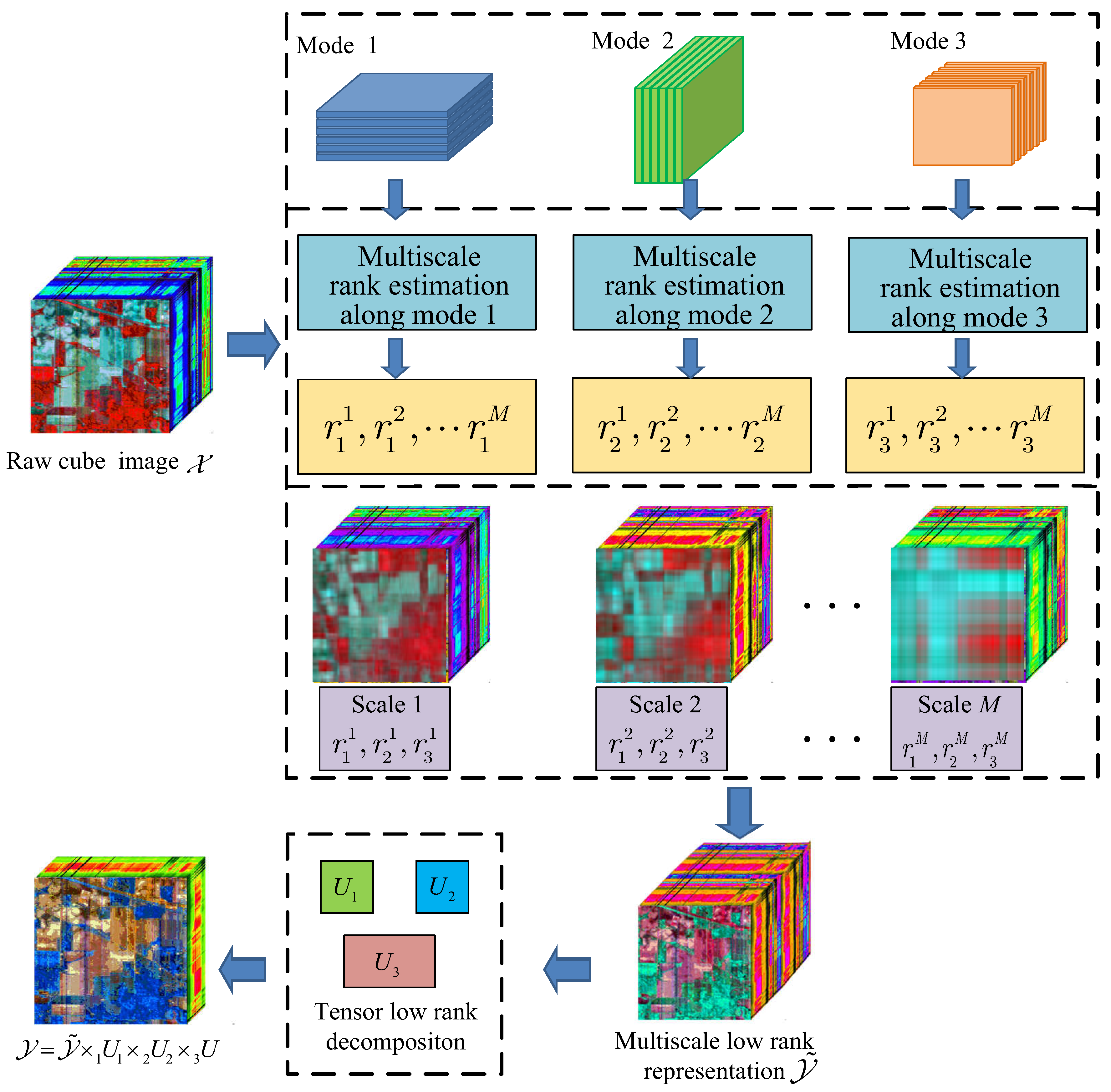
3. Hyperspectral Image Multiscale Low Rank Representation and Fusion

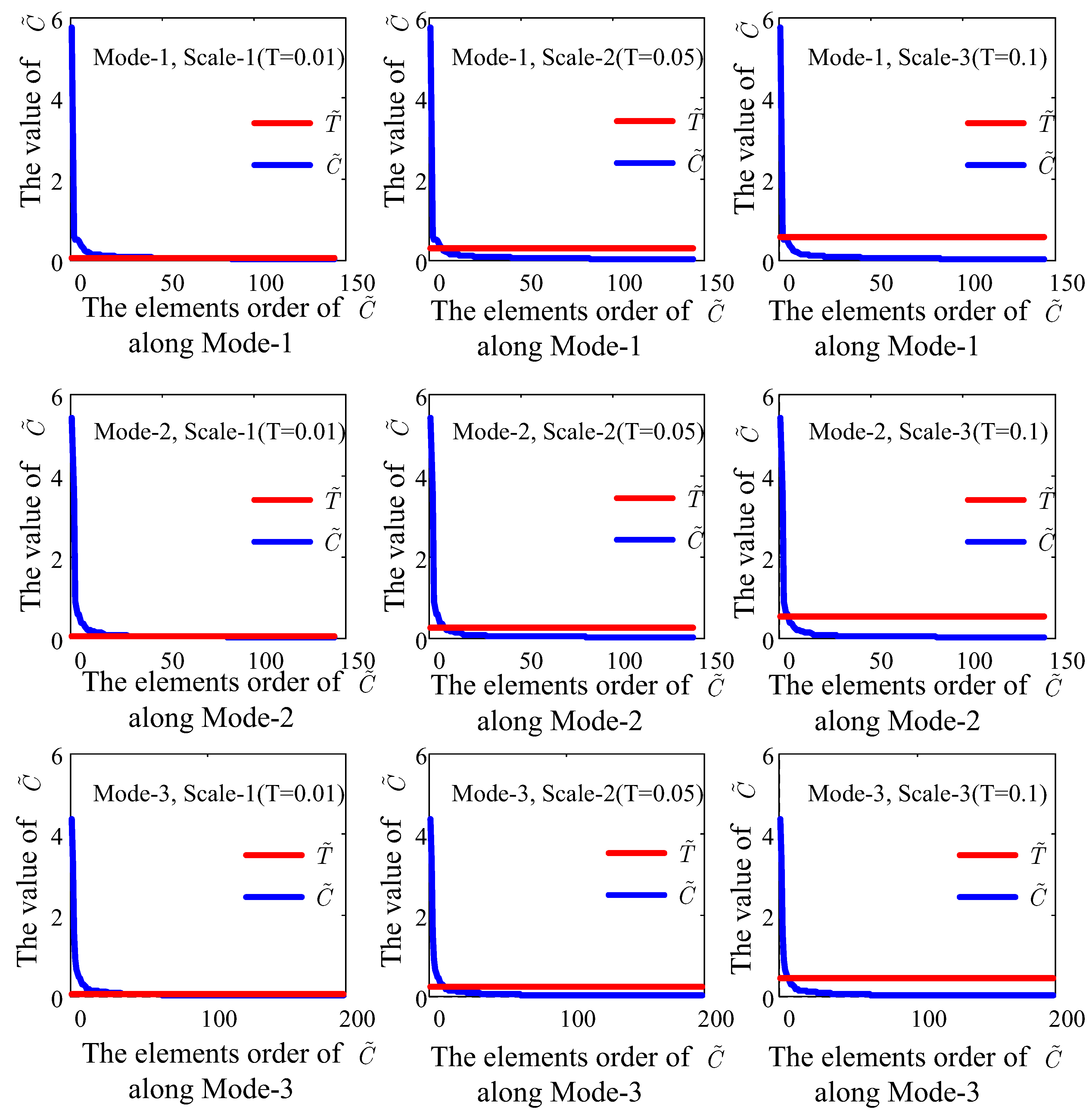
3.1. Adaptive Hypepspectral Image Low Rank Estimating

As discussed above, the rank obtained by tensor low rank decomposition is determined by the number of eigenvectors corresponding to covariance matrix R n R n T . Inspired by the principle of Principal Component Analysis (PCA) [40], the eigenvectors associated with larger eigenvalues are regarded to retain more intrinsic information of the original tensor dataset. By employing the analysis of the eigenvalues correspongding to covariance matrix R n R n T , a novel strategy is proposed here to estimate the rank r n reliably.
Let C be the eigenvalues corresponding to covariance matrix R n R n T , a modified array C ˜ can be calculated by
C ˜ = d ( log ( C ) ) .
By sorting the elements in C ˜ in decreasing order, the rank r n can be determined by
r n = min ( i ) , C ˜ i < T max ( C ˜ ) ,
where T is a given threshold value, and max ( C ˜ ) is the maximum value of C ˜ . The corresponding values of C ˜ on the Indian Pines dataset along each mode are shown in Figure 3. From Figure 3, it can be seen that the elements in the front of C ˜ has large values. It is believed that the eigenvectors corresponding to these elements can preserve the most intrinsic information of the original dataset, which is accordance with the theory of Principal Component Analysis. It can also be seen from Equation (9) that the resulting rank depends on the property of given dataset, so the obtained rank is adaptive for different datasets. In addition, for a given dataset, max ( C ˜ ) is a constant, thus the resulting rank r n can be controlled by parameter T. The smaller the T is, the larger the resulting r n is and the more detailed features may be kept. Conversely, the larger the T is, the smaller the resulting r n is and the more common features of the original hyperspectral image may be preserved. That is to say, different scales low rank feature can be extracted with different T.
Taking the Indian Pines dataset as an example, the estimation of optimal multiscale rank r n m is illustrated in Figure 3, where r n m denotes the optimal rank along mode n of scale m, n = 1 , 2 , 3 denotes the different mode of tensor datasets, m = 1 , 2 , , M is the different low rank scales and M is the number of all scales. Assuming the number of multiscale is 3 and the corresponding threshold T are 0.01, 0.05 and 0.1, the estimating multiscale low rank values along each mode are obtained as shown in the nine subimages of Figure 3. For each mode, the curve of C ˜ is shown in blue, while, for each scale, the values of T max ( C ˜ ) are marked in red lines. The optimal rank shown in the top right corner is obtained by the cross point of the two curves.

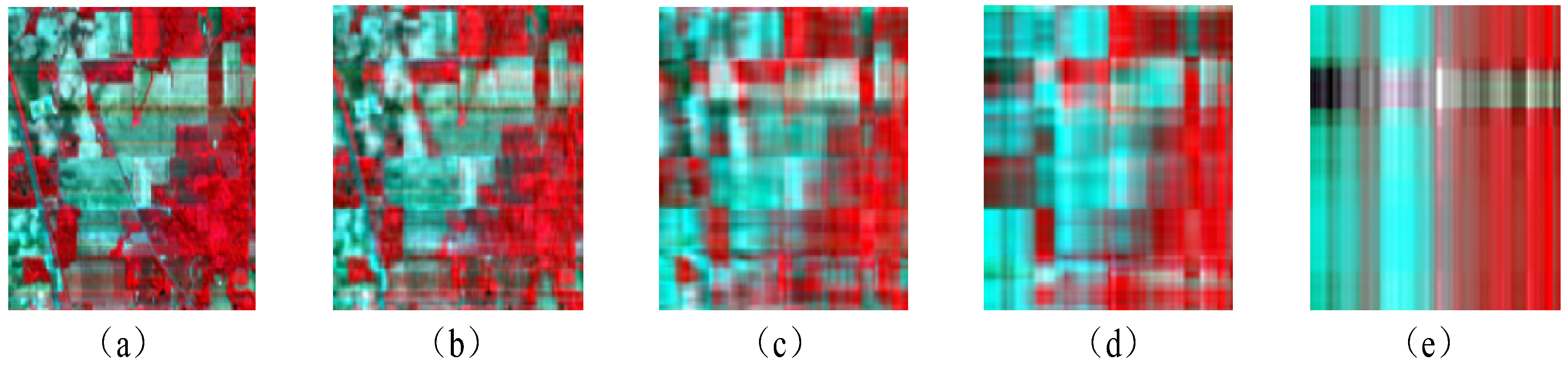
3.2. Hyperspectral Image Multiscale Representation and Low Rank Fusion

Given a hyperspectral image X , by setting different threshold values T m , m = 1 , 2 , , M , where M is the number of different scales. It is easy to compute the resulting rank r n by adopting the rank estimating model. Then, the different scale low rank representation X m , m = 1 , 2 , , M can be obtained by Equation (7). It is noted that different scale low rank representation exhibits different level structure characteristics of hyperspectral images.
It has been proved that a sole scale may not offer sufficient intrinsic structure information for the following processing and different scales may offer complementary and correlated information [37]. Thus, we stack the different level representations together in a spectral domain. For hyperspectral image X R I 1 × I 2 × I 3 , suppose that X ˜ m R I 1 × I 2 × I 3 , m = 1 , 2 , , M are the i t h scale low rank representation. By the stacking all X ˜ i in the spectral domain, the final multiscale low rank representation can be represented as Y ˜ R I 1 × I 2 × ( I 3 × M ) .
For a hyperspectral image, the distinct structures and characteristics will be exhibited more effectively by the multiscale low rank representations. However, different scale representations usually lie on different scales of feature spaces. The strategy of stacking the multiscale low rank representation in the spectral domain faces two disadvantages.
(i) The different scale low rank representations may play different important roles in a specific application, but the stacking strategy treats the different scale representations equally, which ignores the different contributions of different scale representations. (ii) The stacking strategy increases the feature dimensionality which may suffer from the “curse of dimensionality” and the high computational cost.
To fully extract the intrinsic correlative and complementary information offered by the different scale representations, a low rank fusion and dimensionality reduction strategy is proposed. For a hyperspectral image X R I 1 × I 2 × I 3 , Y ˜ R I 1 × I 2 × ( I 3 × M ) is the multiscale low rank representation of X . The low rank fusion and dimensionality reduction Y can be achieved by Equation (10):
Y = Y ˜ × 1 P ˜ 1 × 2 P ˜ 2 × 3 P ˜ 3 ,
where P ˜ n = U ˜ n U ˜ n T , U ˜ n , n = 1 , 2 , 3 consists of the first r n eigenvectors corresponding to the covariance matrix R ˜ n R ˜ n T , R ˜ n is the n-mode flattening matrix of Y ˜ . It is noted that, since Y ˜ consists of some low rank characters of X , for the spatial dimension, U ˜ n , n = 1 , 2 consists of all the eigenvectors corresponding to the covariance matrix R ˜ n R ˜ n T . For the spectral dimension, since the requirement of fusion and dimensionality reduction, P ˜ 3 = Λ 1 / 2 × U ˜ 3 T , Λ is the k × k eigenvector diagonal matrix corresponding to the first k eigenvalues of covariance matrix U ˜ n U ˜ n T ; k is the number of reduced dimensionality.
Overall, the flowchart of the proposed T-MLRD is shown in Figure 1. As shown in Figure 1, for each mode of the raw hyperspectral image, the optimal rank is estimated according to the specified N-scale threshold values, then the low rank representation associated with the optimal rank of scale N is obtained by multiscale low rank decomposition. To fully extract the complementary information of different scale representation, the tensor low rank decomposition strategy is adopted to fuse the different scale representation. Finally, the dimensionality reduction is achieved under the Tucker decomposition framework. The detailed steps of the proposed method are given in Algorithm 1.
Algorithm 1: Proposed T-MLRD algorithm
INPUT:
Original tensor hyperspectral dataset X R I 1 × I 2 × I 3 , threshold T m , m = 1 , 2 , M , reduced dimensionality k.
1:
Estimate the optimal rank r n m of hyperspectral image along mode n of scale m by Equation  (9).
2:
for m=1:M
3:
    Calculate scale m low rank representation by Equation (7).
4:
end for
5:
Stack all the M low rank representation in spectral dimension to construct the multiscale low rank representation Y ˜ .
6:
Calculate the reduced dimensionality dataset Y by Equation (10).
OUTPUT:
Dimensionality reduced of the hyperspectral dataset Y .

4. Experimental Results and Analysis

In this section, experiments are carried out on three real hyperspectral datasets to evaluate the performance of the proposed method.

4.1. Experimental Setup

(i) Hyperspectral dataset: The first dataset is the Indian Pines dataset that was gathered by AVIRIS sensor in June 1992. This scene contains two-thirds agriculture, and one-third forest or other natural perennial vegetation that are designated into 16 classes. The size of this dataset consists of 145 × 145 × 224 with the wavelength range of 0.4–2.5 μ m and the spatial resolution of 20 m. The spectral bands is reduced to 200 by removing the noisy and water absorption bands. Its pseudo-color and corresponding ground truth maps are shown in Figure 4a,b, respectively.
The second dataset named Pavia University was acquired by the Reflective Optics System Imaging Spectrometer (ROSIS) sensor over Pavia University, northern Italy. This is an image of 610 × 340 pixels and 103 spectral bands. The spectral range is from 430 to 860 nm with a geometric resolution of 1.3 m. There are nine classes of land covers in total and its pseudo-color and corresponding ground truth maps are shown in Figure 5a,b, respectively.
The third dataset was collected by the AVIRIS sensor over Salinas Valley, California. This dataset has a size of 512 × 217 × 224 and a high spatial resolution of 3.7 m pixels. Salinas groundtruth contains 16 classes and its pseudo-color and corresponding ground truth maps are illustrated in Figure 6a,b, respectively.
(ii) Comparison methods: To evaluate the performance of the proposed method, several low rank and tensor based methods are selected as the comparison methods, including low-rank graph discriminant analysis (LGDA) [12], group tensor based low rank decomposition (GTLR) [26], tensor based low-rank representation (TLRR) [21], low rank tensor approximation(LRTA) [17] and tensor-based low rank graph with multi-manifold regularization(T-LGMR) [21]. In addition, the original spectral bands and classical PCA are also considered in this letter. For the proposed method, the number of low rank scale is set as 3, and the corresponding threshold parameters are set as [0.01 0.05 0.1].
The Nearest Neighborhood (1NN) classifier and Support Vector Machine (SVM) classifier with Gaussian kernel function are chosen as the classifier to valuate the classification performance of the dimensionality reduced dataset. In addition, 10% labeled samples are randomly selected as the training samples and the remaining as the testing samples. Overall accuracy (OA), Average accuracy (AA), Class-specific Accuracy, Kappa coefficients and the classification maps are reported to show the performance of different methods. To reduce the randomness, each experiment is conducted 10 times and the mean value and the corresponding standard deviation are reported.

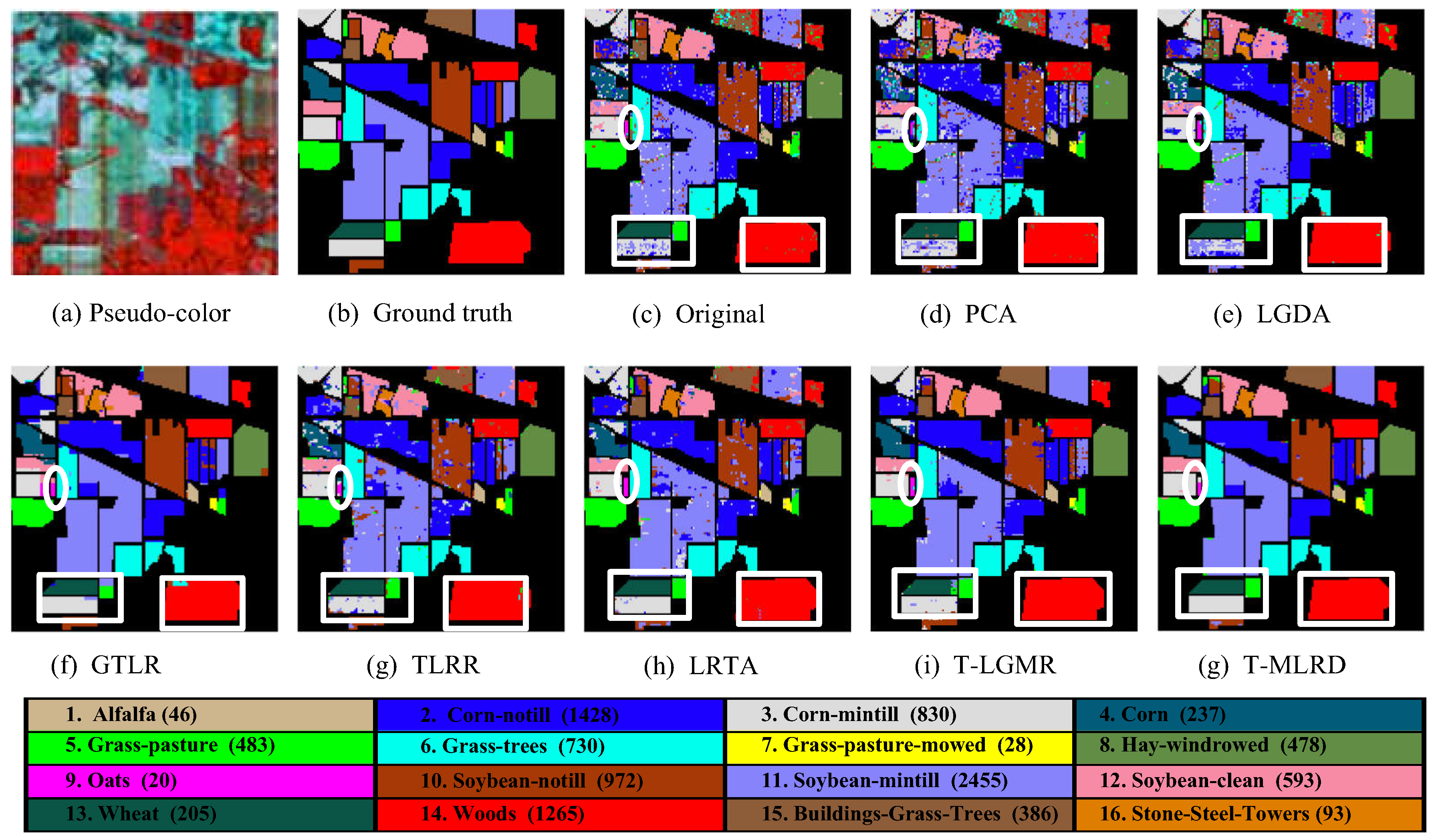
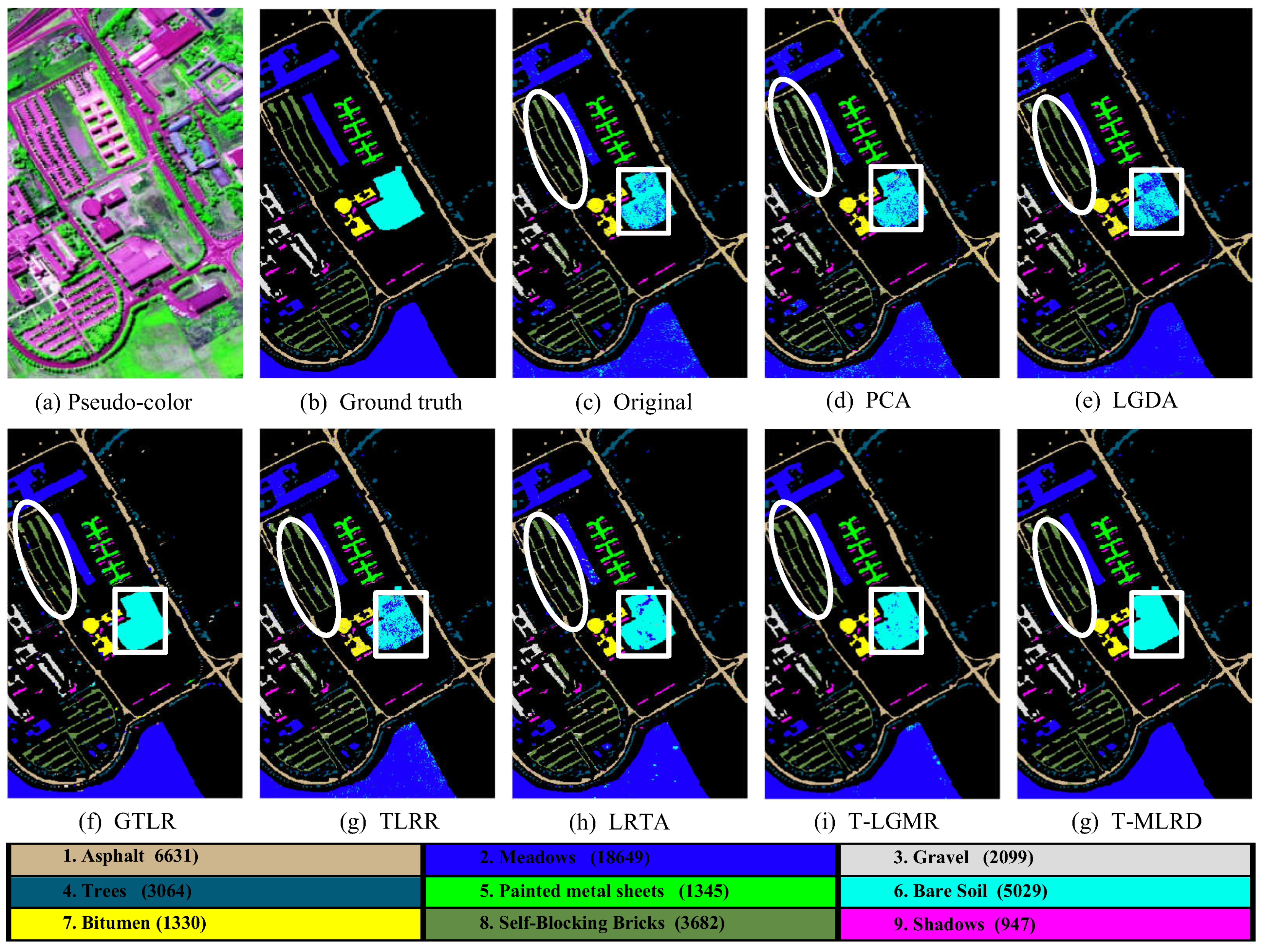
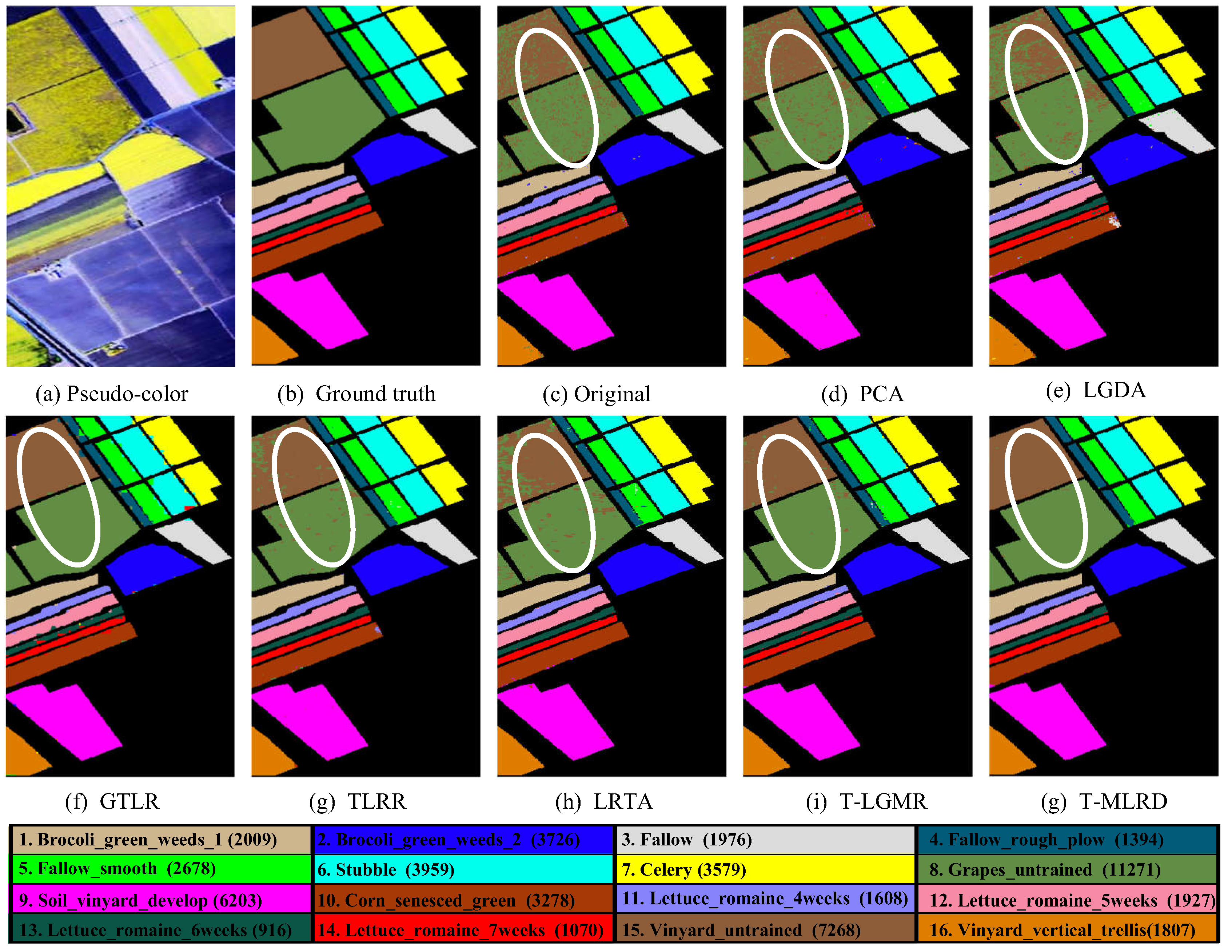
4.2. Classification Results

In this section, classification experiments are carried out on the real hyperspectral datasets. The classification results are shown in Table 1, Table 2 and Table 3 and the classification maps are shown in Figure 4, Figure 5 and Figure 6.
For the Indian Pines dataset, it can be seen from Table 1 that the proposed method achieves much higher classification accuracy than comparison methods. For example, the proposed method achieves about 2% and 3% higher accuracy than the second best method in terms of OA and AA. It is noted that, for class 13, the proposed method achieves almost 100% classification accuracy. Figure 4 shows the classification maps of different methods on Indian Pines dataset. It can be observed from Figure 4 that the proposed method can obtain promising performance for the classes with good spatial consistencymarked by white rectangle). In addition, for small samples classes, such as class 7 and class 9, the proposed method can also achieve satisfactory classification results.
For the Pavia University dataset, the advantages of the proposed method over the comparison methods are also evident. It can be seen from Figure 5 that the proposed method achieves good regional uniformity in the area marked by white rectangle which may be easily corrupted by spot noise. Furthermore, for the ribbon area (marked by the ellipse), the proposed method can also achieve promising performance.
For Salinas dataset, the land covers in this scene all have large sample numbers and good region consistency. All of the comparison methods achieve satisfactory classification performance. It is noted that class 8 and class 15 are easy to confuse (marked by the white ellipse in Figure 5) and there are many mis-classified noises in the classification maps obtained by the vector-based methods (Original, PCA and LGDA). For tensor-based methods (GTLR, TLRR, LRTA, T-LGMR and T-MLRD), by utilizing spatial neighborhod information, the region consistency of these two land-covers is obviously superior to that of vector-based methods. In addition, it can be seen from the classification maps that the proposed method achieves the best classification performance by fusing multiscale low rank structure information.

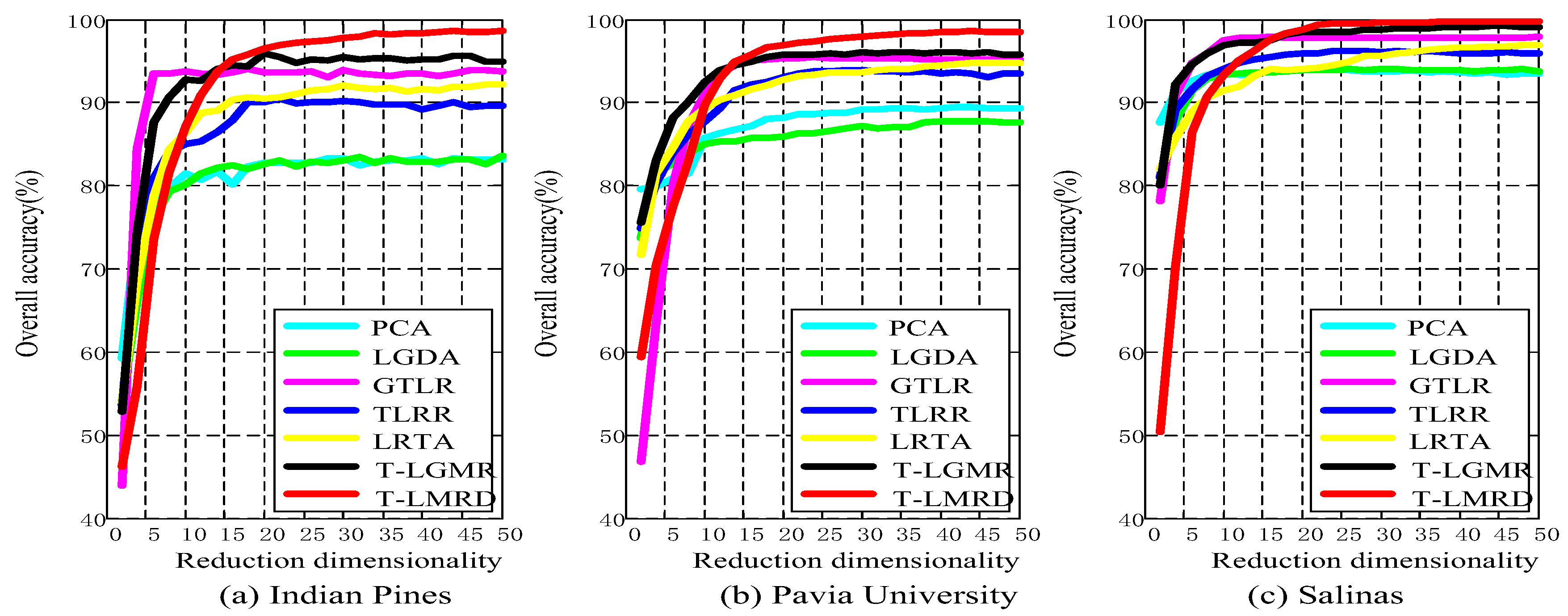
4.3. Analysis of Different Reduced Dimensionality

In this section, experiments are carried out to evaluate the classification performance with different dimensionalities. It can be seen from Figure 7 that the proposed method achieves better performance than the comparison methods when the reduced dimensionality is larger than 15. In addition, the performance of the proposed method can be further improved with the increase of dimensionality while the overall accuracy of the comparison methods may remain stable. This further demonstrates that the proposed method can reduce the dimensionality and preserve rich information of the original dataset.

4.4. Analysis of Computational Costs

In this section, experiments are carried out on three hyperspectral images to demonstrate the computational efficiency of the proposed method. All the experiments are accomplished using Matlab R2014a on a PC with Intel Core i5-5490 CPU and 8 GB RAM. The mean time (in terms of seconds) of ten repetitions of all comparison methods is listed in Table 4.
In can be seen from Table 4 that the running time of vector samples based methods whose solutions do not need to compute the optimal factor matrix for each mode are shorter than tensor sample based methods. For tensor based methods, due to the iterative strategy of obtaining the optimal rank for each mode, TLRR and T-LGMR cost the longest running time. Since the best rank for each mode are specified directly in GTLR, LRTA and T-LMRD, the cost time of these three methods are almost the same. Compared with the excellent performance, the running time of T-LGMR is acceptable.

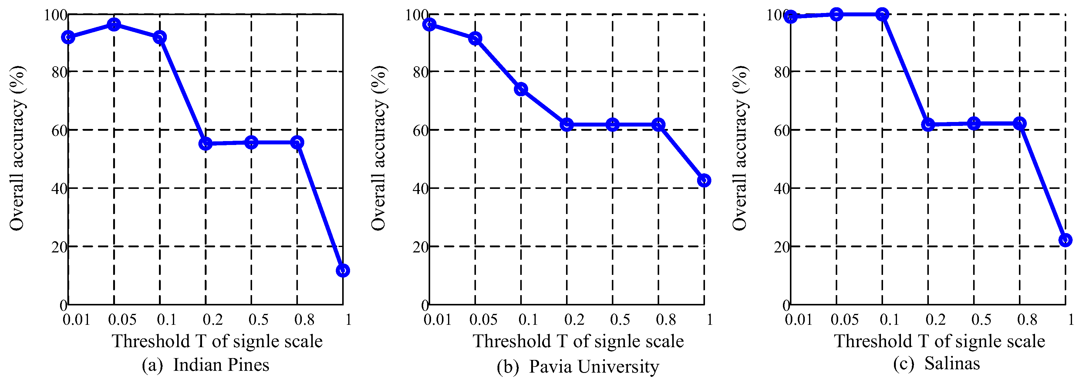
4.5. Analysis of Different Scales

In previous experiments, the number of multiscales is set as 3, and the corresponding threshold parameters are set as [0.01 0.05 0.1], respectively. In this part, the number of low rank scales is expanded and its effect on the overall accuracy is analyzed. The number of low rank scales is set as 7 and the corresponding threshold parameters space is set as [0.01 0.05 0.1 0.2 0.5 0.8 1.0]. The classification results of single scale low rank representation are shown in Figure 8 and the classification results of multiscale low rank representation are reported in Figure 8.
It can be seen from Figure 8 that, for a single scale, the correlation of overall accuracy and parameter T is uncertain, which suggests that the optimal single threshold is difficult to be determined. For example, for the Indian Pine dataset, the overall accuracy associated with the first three thresholds is about the same and the second threshold is the optimal one, but, for Pavia University dataset, the first threshold is the optimal one while the overall accuracy associated with the second and third one decreases rapidly. This further reveals that the threshold parameter T is difficult to be determined in real application. Figure 9 shows the classification results with different sizes of multiscale on the three hyperspectral datasets. There are seven pointed multiscale threshold values of the x axis, i.e., M T 1 M T 7 , the correspongding multiscale threshold values are listed in the legend table of Figure 9. It is seen that the overall accuracy increases dramatically at the beginning and, when the number of multiscales is larger than 3, the curve increases slowly and then remains stable. Thus, the number of multiscale being set as 3 in the experiments is reasonable.

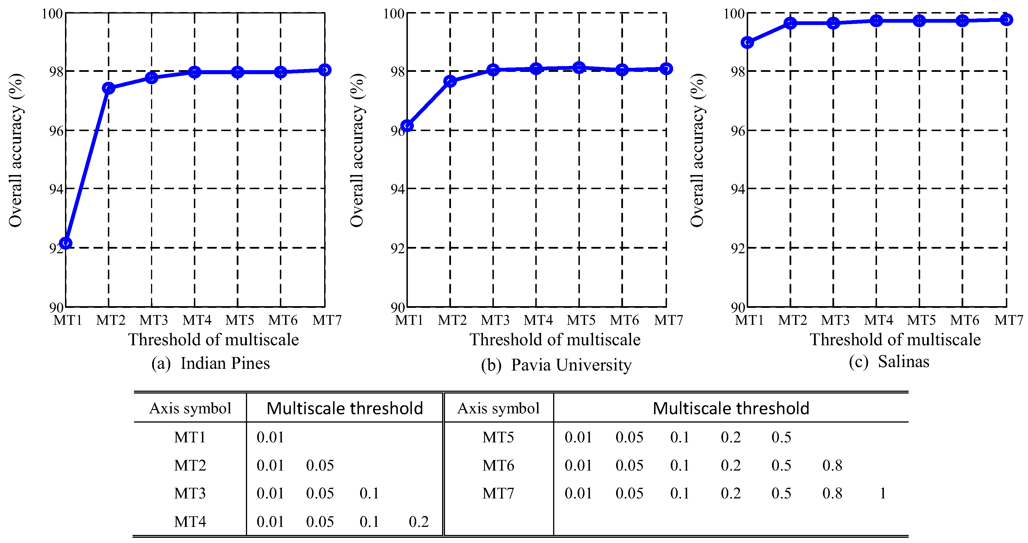
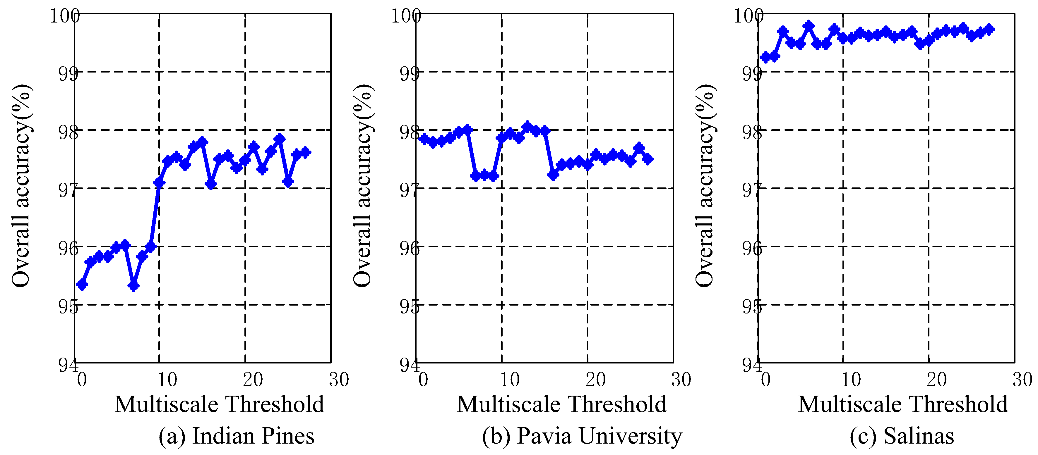
4.6. Analysis of Multiscale Threshold Values

In the experiments above, the number of different scale is set as 3 and the corresponding threshold values are set as 0.01, 0.05 and 0.1. To investigate the effect of the threshold values T, we extend the threshold values space of the three scales and discuss the effect of threshold values on the overall classification accuracy. Specifically, [0.005 0.01 0.015], [0.03 0.05 0.07] and [ 0.08 0.1 0.12] are set as the different threshold values for scale 1, scale 2 and scale 3, respectively. The final multiscale threshold values are constructed by selecting one from the three values for each scale, thus the resulting threshold values space is composed of 27 different threshold values combinations, which are shown in Table 5. Classification experiments are carried out with 27 different multiscale threshold values and the corresponding overall classification accuracies are shown in Figure 10. It can be seen from Figure 10 that the overall accuracy varies slightly within the whole threshold values space. For example, the maximum change of overall accuracy on Salinas is only 0.53. This shows the robustness of the proposed method against the threshold values and further demonstrates the fact that different scales’ low rank representation can offer complementary structure information.

5. Discussion

5.1. Classification Results of Different Reduced Dimensionality

It can be seen from the analysis of different reduced dimensionality that, when the reduced dimensionality is larger than 20, the proposed method achieves the best classification performance of all compared methods, while, when the reduced dimensionality k is less than 15, the accuracy performance of T-LMRD is worse than some of the compared methods. This is mainly due to the stacking strategy of all single low rank representations on a spectral domain possibly leading to a high dimensionality of multiscale low rank representation. Taking the Indian Pines dataset, for example, the original dimensionality is 200 while the dimensionality of multiscale low rank representation is 600 when the number of scale is set as 3. If we extract the feature representation with an extremely low dimensionality, such as 5 or 10, from such a high feature space, the intrinsic information of multiscale representation may not be fully preserved by the resulting low dimensionality feature representation, so the classification performance of the T-MLRD may be worse than the compared methods when the dimensionality is extremely low. Considering the outstanding performance with slightly higher dimensionality, the proposed T-MLRD is still a rather good dimensionality reduction method.

5.2. Multiscale Threshold Values

From the analysis of different scales, it can be observed that there are obvious advantages of multiscale over the optimal single scale in terms of classification overall accuracy, which demonstrates the superiority of multiscale analysis. Furthermore, Figure 8 and Figure 9 shows that, when the number of scales is larger than 3, the overall classification accuracies of single scale are extremely low, but, if these single scale features are fused into the multiscale feature space, the resulting performance may also be improved. This further reveals the complementarity of the features obtained from different scales.

6. Conclusions

In this paper, a novel tensor based multiscale low rank decomposition method was proposed for hyperspectral images dimensionality reduction and classification. With a novel multiscale rank estimating method that can automatically estimate the optimal multiscale rank along each mode of hyperspectral images, the multiscale low rank decomposition is employed to obtain a multiscale low rank representation of original hyperspectral images. Then, the low rank tensor approximation strategy is employed to fuse the multiscale low rank feature representation and achieve dimensionality reduction. Furthermore, as an unsupervised dimensionality reduction method, the proposed T-MLRD is able to extract the intrinsic structure information from original cube hyperspectral images directly, which needs no labeled samples and avoids the complicated tensor training samples construction, which makes the T-MLRD more practical. Experimental results on real hyperspectral images demonstrate the advantages of the proposed method over the state-of-the-art approaches.

Author Contributions

Methodology, J.A. and X.Z.; Resources, J.G.; Validation, J.L. and Y.S.; Writing—original draft, J.A.; Writing—review and editing, X.Z.

Funding

This work was supported in part by the National Natural Science Foundation of China under Grant No. 61772400.

Conflicts of Interest

All of the authors declare no conflict of interest.

References

  1. Zhang, X.; Gao, Z.; Jiao, L.; Zhou, H. Multifeature Hyperspectral Image Classification With Local and Nonlocal Spatial Information via Markov Random Field in Semantic Space. IEEE Trans. Geosci. Remote Sens. 2017. [Google Scholar] [CrossRef]
  2. Zhang, X.; Liang, Y.; Li, C.; Ning, H.; Jiao, L.; Zhou, H. Recursive Autoencoders-Based Unsupervised Feature Learning for Hyperspectral Image Classification. IEEE Geosci. Remote Sens. Lett. 2017, 14, 1928–1932. [Google Scholar] [CrossRef] [Green Version]
  3. Kwon, H.; Nasrabadi, N.M. Kernel Matched Subspace Detectors for Hyperspectral Target Detection. IEEE Trans. Pattern Anal. Mach. Intell. 2005, 28, 178–194. [Google Scholar] [CrossRef]
  4. Manolakis, D.; Siracusa, C.; Shaw, G. Hyperspectral subpixel target detection using the linear mixing model. Geosci. Remote Sens. IEEE Trans. 2001, 39, 1392–1409. [Google Scholar] [CrossRef]
  5. Zhang, K.; Wang, M.; Yang, S.; Jiao, L. Spatial Spectral-Graph-Regularized Low-Rank Tensor Decomposition for Multispectral and Hyperspectral Image Fusion. IEEE J. Sel. Top. Appl. Earth Obs. Remote Sens. 2018, 11, 1030–1040. [Google Scholar] [CrossRef]
  6. Zhang, X.; Li, C.; Zhang, J.; Chen, Q.; Feng, J.; Jiao, L.; Zhou, H. Hyperspectral Unmixing via Low-Rank Representation with Space Consistency Constraint and Spectral Library Pruning. Remote Sens. 2018, 10, 339. [Google Scholar] [CrossRef]
  7. Gao, Y.; Wang, X.; Cheng, Y.; Wang, Z.J. Dimensionality Reduction for Hyperspectral Data Based on Class-Aware Tensor Neighborhood Graph and Patch Alignment. IEEE Trans. Neural Netw. Learn. Syst. 2015, 26, 1582–1593. [Google Scholar] [PubMed]
  8. Feng, F.; Li, W.; Du, Q.; Zhang, B. Dimensionality Reduction of Hyperspectral Image with Graph-Based Discriminant Analysis Considering Spectral Similarity. Remote Sens. 2017, 9, 323. [Google Scholar] [CrossRef]
  9. Liu, S.; Du, Q.; Tong, X.; Samat, A.; Pan, H.; Ma, X. Band Selection-Based Dimensionality Reduction for Change Detection in Multi-Temporal Hyperspectral Images. Remote Sens. 2017, 9, 1008. [Google Scholar] [CrossRef]
  10. Liu, G.; Lin, Z.; Yan, S.; Sun, J.U.; Yong, Y.U.; Yi, M.A. Robust Recovery of Subspace Structures by Low-Rank Representation. IEEE Trans. Pattern Anal. Mach. Intell. 2012, 35, 171–184. [Google Scholar] [CrossRef] [PubMed] [Green Version]
  11. Zheng, Y.; Jiao, L.; Shang, R.; Hou, B.; Zhang, X. Local Collaborative Representation With Adaptive Dictionary Selection for Hyperspectral Image Classification. IEEE Geosci. Remote Sens. Lett. 2016, 13, 1482–1486. [Google Scholar] [CrossRef]
  12. Wei, L.; Liu, J.; Qian, D. Sparse and Low-Rank Graph for Discriminant Analysis of Hyperspectral Imagery. IEEE Trans. Geosci. Remote Sens. 2016, 54, 4094–4105. [Google Scholar]
  13. Rasti, B.; Ghamisi, P.; Plaza, J.; Plaza, A. Fusion of Hyperspectral and LiDAR Data Using Sparse and Low-Rank Component Analysis. IEEE Trans. Geosci. Remote Sens. 2017, 55, 6354–6365. [Google Scholar] [CrossRef] [Green Version]
  14. Zhao, Y.Q.; Yang, J. Hyperspectral Image Denoising via Sparse Representation and Low-Rank Constraint. IEEE Trans. Geosci. Remote Sens. 2014, 53, 296–308. [Google Scholar] [CrossRef]
  15. Gao, L.; Yao, D.; Li, Q.; Zhuang, L.; Zhang, B.; Bioucas-Dias, J. A New Low-Rank Representation Based Hyperspectral Image Denoising Method for Mineral Mapping. Remote Sens. 2017, 9, 1145. [Google Scholar] [CrossRef]
  16. Li, W.; Du, Q. Laplacian Regularized Collaborative Graph for Discriminant Analysis of Hyperspectral Imagery. IEEE Trans. Geosci. Remote Sens. 2016, 54, 7066–7076. [Google Scholar] [CrossRef]
  17. Renard, N.; Bourennane, S.; Blanc-Talon, J. Denoising and Dimensionality Reduction Using Multilinear Tools for Hyperspectral Images. IEEE Geosci. Remote Sens. Lett. 2008, 5, 138–142. [Google Scholar] [CrossRef]
  18. Zhong, Z.; Fan, B.; Duan, J.; Wang, L.; Ding, K.; Xiang, S.; Pan, C. Discriminant Tensor Spectral Spatial Feature Extraction for Hyperspectral Image Classification. IEEE Geosci. Remote Sens. Lett. 2017, 12, 1028–1032. [Google Scholar] [CrossRef]
  19. Xian, G.; Xin, H.; Zhang, L.; Zhang, L.; Plaza, A.; Benediktsson, J.A. Support Tensor Machines for Classification of Hyperspectral Remote Sensing Imagery. IEEE Trans. Geosci. Remote Sens. 2016, 54, 3248–3264. [Google Scholar]
  20. Makantasis, K.; Doulamis, A.D.; Doulamis, N.D.; Nikitakis, A. Tensor-Based Classification Models for Hyperspectral Data Analysis. IEEE Trans. Geosci. Remote Sens. 2018, 56, 6884–6898. [Google Scholar] [CrossRef]
  21. An, J.; Zhang, X.; Zhou, H.; Jiao, L. Tensor-Based Low-Rank Graph With Multimanifold Regularization for Dimensionality Reduction of Hyperspectral Images. IEEE Trans. Geosci. Remote Sens. 2018, 56, 4731–4746. [Google Scholar] [CrossRef]
  22. Wang, Y.; Chen, X.; Han, Z.; He, S. Hyperspectral Image Super-Resolution via Nonlocal Low-Rank Tensor Approximation and Total Variation Regularization. Remote Sens. 2017, 9, 1286. [Google Scholar] [CrossRef]
  23. Li, C.; Ma, Y.; Huang, J.; Mei, X.; Ma, J. Hyperspectral image denoising using the robust low-rank tensor recovery. J. Opt. Soc. Am. Opt. Image Sci. Vis. 2015, 32, 1604–1612. [Google Scholar] [CrossRef] [PubMed]
  24. Du, B.; Zhang, M.; Zhang, L.; Hu, R.; Tao, D. PLTD: Patch-Based Low-Rank Tensor Decomposition for Hyperspectral Images. IEEE Trans. Multimed. 2017, 19, 67–79. [Google Scholar] [CrossRef]
  25. Dian, R.; Li, S.; Fang, L. Learning a Low Tensor-Train Rank Representation for Hyperspectral Image Super-Resolution. IEEE Trans. Neural Netw. Learn. Syst. 2019. [Google Scholar] [CrossRef] [PubMed]
  26. An, J.; Zhang, X.; Jiao, L.C. Dimensionality Reduction Based on Group-Based Tensor Model for Hyperspectral Image Classification. IEEE Geosci. Remote Sens. Lett. 2016, 13, 1497–1501. [Google Scholar] [CrossRef]
  27. Pan, L.; Li, H.C.; Deng, Y.J.; Zhang, F.; Chen, X.D.; Du, Q. Hyperspectral Dimensionality Reduction by Tensor Sparse and Low-Rank Graph-Based Discriminant Analysis. Remote Sens. 2017, 9, 452. [Google Scholar] [CrossRef]
  28. Fan, H.; Chen, Y.; Guo, Y.; Zhang, H.; Kuang, G. Hyperspectral Image Restoration Using Low-Rank Tensor Recovery. IEEE J. Sel. Top. Appl. Earth Obs. Remote Sens. 2017, 10, 4589–4604. [Google Scholar] [CrossRef]
  29. Fu, Y.; Gao, J.; Tien, D.; Lin, Z.; Hong, X. Tensor LRR and Sparse Coding-Based Subspace Clustering. IEEE Trans. Neural Networks Learn. Syst. 2016, 27, 2120–2133. [Google Scholar] [CrossRef] [Green Version]
  30. Yang, J.; Qian, J. Hyperspectral Image Classification via Multiscale Joint Collaborative Representation With Locally Adaptive Dictionary. IEEE Geosci. Remote Sens. Lett. 2018, 15, 112–116. [Google Scholar] [CrossRef]
  31. Yu, H.; Gao, L.; Liao, W.; Zhang, B.; Pizurica, A.; Philips, W.; Yu, H.; Gao, L.; Liao, W.; Zhang, B. Multiscale Superpixel-Level Subspace-Based Support Vector Machines for Hyperspectral Image Classification. IEEE Geosci. Remote Sens. Lett. 2017, 14, 1–5. [Google Scholar] [CrossRef]
  32. Zhang, C.; Zheng, Y.; Feng, C. Spectral Spatial Classification of Hyperspectral Images Using Probabilistic Weighted Strategy for Multifeature Fusion. IEEE Geosci. Remote Sens. Lett. 2016, 13, 1562–1566. [Google Scholar]
  33. Tong, F.; Tong, H.; Jiang, J.; Zhang, Y. Multiscale Union Regions Adaptive Sparse Representation for Hyperspectral Image Classification. Remote Sens. 2017, 9, 872. [Google Scholar] [CrossRef]
  34. He, N.; Paoletti, M.E.; Haut, J.M.; Fang, L.; Li, S.; Plaza, A.; Plaza, J. Feature Extraction With Multiscale Covariance Maps for Hyperspectral Image Classification. IEEE Trans. Geosci. Remote Sens. 2019, 57, 1–15. [Google Scholar] [CrossRef]
  35. Liang, M.; Jiao, L.; Yang, S.; Fang, L.; Hou, B.; Chen, H. Deep Multiscale Spectral-Spatial Feature Fusion for Hyperspectral Images Classification. IEEE J. Sel. Top. Appl. Earth Obs. Remote Sens. 2018, 11, 1–14. [Google Scholar] [CrossRef]
  36. Li, H.; Song, Y.; Chen, C.L.P. Hyperspectral Image Classification Based on Multiscale Spatial Information Fusion. IEEE Trans. Geosci. Remote Sens. 2017, 55, 5302–5312. [Google Scholar] [CrossRef]
  37. Fang, L.; Li, S.; Kang, X.; Benediktsson, J.A. Spectral Spatial Hyperspectral Image Classification via Multiscale Adaptive Sparse Representation. IEEE Trans. Geosci. Remote Sens. 2014, 52, 7738–7749. [Google Scholar] [CrossRef]
  38. Zhang, S.; Li, S.; Fu, W.; Fang, L. Multiscale Superpixel-Based Sparse Representation for Hyperspectral Image Classification. Remote Sens. 2017, 9, 139. [Google Scholar] [CrossRef]
  39. Lathauwer, L.D.; Moor, B.D.; Vandewalle, J. On the best rank-1 and rank-(R1, R2,...,RN ) approximation of higher-order tensor. Siam J. Matrix Anal. Appl. 2000, 21, 1324–1342. [Google Scholar] [CrossRef]
  40. Jolliffe, I.T. Principal Component Analysis; Springer: Berlin, Germany, 2010; pp. 41–64. [Google Scholar]
Figure 1. The schematic illustration of T-MLRD.The proposed T-MLRD consists of four steps: (1) estimate the optimal rank for each mode of the raw hyperspectral image according to the specified N-scale threshold values. (2) Construct the single low rank representation associated to the optimal rank of scale N. (3) Fuse the different scale representation tensor low rank decomposition strategy. (4) The dimensionality reduction is achieved under the Tucker decomposition framework.
Remotesensing 11 01485 g001
Figure 2. The low rank representation with different rank along each mode on Indian Pines dataset. (a) original pseudo-color map; (b) rank = 30 along each mode; (c) rank = 10 along each mode; (d) rank = 5 along each mode; (e) rank = 2 along each mode.
Remotesensing 11 01485 g002
Figure 3. The estimation of optimal multiscale rank along each mode on Indian Pines.
Remotesensing 11 01485 g003
Figure 4. Classification maps of different methods on the Indian Pines dataset.
Remotesensing 11 01485 g004
Figure 5. Classification maps of different methods on the Pavia University dataset.
Remotesensing 11 01485 g005
Figure 6. Classification maps of different methods on the Salinas dataset.
Remotesensing 11 01485 g006
Figure 7. Overall accuracy with different dimensionalities. (a) Indian Pines; (b) Pavia University; (c) Salinas.
Remotesensing 11 01485 g007
Figure 8. Overall accuracy of single scale low rank representation.
Remotesensing 11 01485 g008
Figure 9. Overall accuracy of multiscale low rank representation.
Remotesensing 11 01485 g009
Figure 10. Overall classification accuracy with different multiscale threshold values.
Remotesensing 11 01485 g010
Table 1. Classification results on the Indian Pines dataset (Reduction Dimensionality = 30).
ClassOriginalPCALGDASGDASLGDATLRRTSRPT-SLG
SVM1NNSVM1NNSVM1NNSVM1NNSVM1NNSVM1NNSVM1NNSVM1NN
173.75
±10.68
67.92
±12.89
63.13
±10.29
59.79
±10.91
65.73
±12.71
65.10
±7.68
84.38
±10.72
83.75
±9.10
79.17
±8.07
77.50
±5.78
83.13
±10.18
80.83
±7.53
93.33
±4.52
95.42
±4.97
96.04
±4.41
94.58
±4.68
283.77
±1.17
63.33
±1.42
76.60
±2.16
62.40
±3.19
76.64
±2.70
67.35
±3.10
91.12
±1.73
91.42
±1.41
90.47
±1.40
86.57
±1.49
90.53
±1.59
90.41
±1.44
94.57
±1.27
94.09
±1.24
96.83
±1.59
98.47
±0.75
378.93
±2.39
62.37
±1.72
66.15
±3.12
57.55
±2.14
64.91
±2.93
62.38
±2.95
88.21
±5.08
89.01
±3.26
83.28
±1.51
74.77
±2.29
84.88
±2.69
86.39
±1.61
91.57
±3.06
92.59
±3.10
97.15
±1.07
97.39
±1.29
470.10
±7.43
46.10
±7.81
50.19
±5.46
44.52
±3.73
74.02
±8.36
44.17
±5.30
87.29
±3.95
87.48
±4.28
77.33
±5.44
76.95
±4.28
86.71
±6.32
86.95
±3.27
90.95
±2.63
87.62
±5.76
98.19
±1.49
97.81
±2.27
594.05
±1.63
91.59
±2.01
88.28
±2.73
87.74
±2.70
91.15
±2.55
88.81
±2.36
96.69
±2.01
96.51
±2.18
93.69
±2.28
93.87
±3.07
96.40
±2.26
95.10
±2.24
94.59
±3.35
95.48
±3.64
96.2
±1.97
95.44
±1.91
696.67
±1.11
94.67
±1.29
94.49
±1.43
93.91
±1.78
95.05
±2.38
94.07
±1.44
95.98
±3.90
96.59
±3.13
96.88
±2.37
93.63
±2.47
99.54
±0.57
99.79
±0.19
98.07
±1.27
97.32
±1.27
99.64
±0.29
99.75
±0.22
778.26
±10.2
83.48
±7.78
77.39
±10.07
82.61
±7.53
78.70
±14.08
75.87
±14.45
99.50
±1.58
99.10
±2.02
83.48
±3.64
76.52
±10.01
87.39
±8.31
85.65
±10.6
88.70
±16.1
77.39
±16.6
90.87
±7.39
93.91
±7.33
898.18
±0.89
98.05
±0.83
97.34
±1.15
96.95
±1.14
98.20
±0.79
98.15
±0.73
97.36
±3.98
97.36
±3.98
99.50
±0.10
99.68
±0.20
99.38
±1.34
99.40
±1.05
99.64
±0.20
99.64
±0.20
99.86
±0.29
99.75
±0.31
972.22
±17.10
57.78
±9.30
20.56
±9.64
23.33
±13.33
50.83
±21.17
41.39
±18.3
36.36
±24.27
39.43
±31.7
61.11
±25.76
66.67
±23.9
83.33
±23.72
91.67
±9.53
78.89
±14.3
82.22
±17.3
90.56
±23.1
80.00
±14.74
1078.99
±2.35
74.28
±2.39
76.00
±1.93
70.49
±2.41
67.07
±5.45
75.96
±3.91
92.79
±3.75
92.61
±3.38
82.46
±3.27
73.87
±3.08
86.96
±2.04
92.22
±1.09
92.74
±1.45
94.76
±0.99
95.88
±2.05
96.6
±1.09
1184.07
±1.43
77.03
±2.13
83.37
±1.04
75.27
±0.86
84.77
±2.04
78.07
±1.76
98.54
±1.34
98.22
±1.46
88.54
±1.70
88.71
±0.73
89.58
±1.68
94.17
±0.92
95.61
±1.27
96.88
±1.39
98.57
±0.48
99.17
±0.37
1284.42
±2.62
58.80
±4.19
66.34
±3.54
53.26
±2.78
75.7
±5.41
58.89
±3.31
80.24
±5.42
81.39
±3.23
88.01
±4.10
76.09
±3.27
91.05
±2.90
90.16
±2.08
94.64
±2.15
94.24
±1.83
95.94
±1.40
95.91
±2.01
1399.05
±0.69
98.00
±1.36
96.11
±2.32
96.68
±1.94
98.29
±2.02
97.74
±1.88
94.89
±8.06
94.89
±8.06
99.26
±0.29
98.42
±0.64
99.30
±1.16
98.70
±1.89
97.37
±2.93
96.00
±4.20
100
±0
99.95
±0.16
1494.64
±1.43
93.06
±1.39
95.15
±0.84
93.17
±0.92
96.84
±0.74
92.64
±1.63
96.73
±3.12
96.13
±3.14
95.45
±1.72
97.25
±0.47
96.35
±1.33
98.11
±0.75
98.30
±1.21
99.02
±0.51
99.35
±0.54
99.09
±0.75
1561.05
±6.07
42.40
±3.74
51.17
±4.12
38.48
±1.87
51.84
±4.71
39.80
±5.67
93.33
±4.53
93.33
±4.53
79.53
±3.27
79.47
±5.33
85.94
±5.13
86.64
±3.73
96.14
±1.67
95.85
±1.84
97.13
±2.48
98.83
±1.37
1690.82
±3.37
93.18
±3.16
55.06
±9.39
89.18
±4.46
87.65
±4.84
86.35
±5.17
61.41
±12.8
64.82
±12.04
88.47
±4.19
85.65
±1.93
95.65
±4.44
94.12
±5.08
90.35
±4.19
91.76
±2.20
90.94
±4.79
92.47
±5.89
OA85.67
±0.37
76.12
±0.69
80.35
±0.43
73.87
±0.21
81.72
±1.01
76.59
±1.23
93.43
±0.66
93.54
±0.74
89.53
±0.39
86.78
±0.59
91.57
±0.47
93.39
±0.45
95.31
±0.65
95.76
±0.54
97.78
±0.44
98.22
±0.25
AA83.71
±0.49
75.13
±1.14
72.33
±1.61
70.33
±1.29
78.59
±2.06
72.92
±2.27
86.22
±2.50
87.62
±2.74
86.66
±1.87
84.10
±1.67
91.09
±1.56
91.99
±1.22
93.47
±2.40
93.14
±2.44
96.45
±1.97
96.19
±1.59
Kappa0.85
±0
0.75
±0.01
0.8
±0
0.73
±0
0.81
±0.01
0.76
±0.01
0.93
±0.01
0.93
±0.01
0.89
±0
0.86
±0.01
0.91
±0
0.93
±0
0.95
±0.01
0.96
±0.01
0.98
±0
0.98
±0
Table 2. Classification results on Pavia University dataset (reduction dimensionality = 30).
ClassOriginalPCALGDASGDASLGDATLRRTSRPT-SLG
SVM1NNSVM1NNSVM1NNSVM1NNSVM1NNSVM1NNSVM1NNSVM1NN
189.65
±0.69
75.92
±0.99
89.65
±0.6
77.97
±0.79
92.62
±0.76
84.00
±1.30
94.21
±1.32
94.61
±1.03
94.08
±0.83
70.67
±2.85
93.67
±0.55
96.77
±0.43
96.41
±0.83
92.38
±1.23
96.89
±0.63
98.75
±0.32
295.54
±0.63
95.27
±0.15
94.5
±0.56
94.92
±0.25
97.10
±0.44
92.11
±0.83
99.30
±0.24
99.30
±0.29
97.75
±0.53
97.97
±0.40
98.22
±0.18
99.56
±0.11
99.18
±0.16
99.73
±0.09
99.75
±0.10
99.92
±0.06
370.92
±2.02
60.30
±1.60
71.2
±1.8
61.01
±1.6
69.54
±2.17
59.17
±2.66
94.84
±1.25
94.84
±1.18
76.82
±2.95
68.93
±1.93
76.69
±1.52
91.55
±1.24
85.08
±1.52
89.09
±1.32
97.01
±1.10
99.31
±0.34
492.74
±1.17
83.29
±1.40
92.29
±0.54
84.26
±0.97
88.98
±1.64
81.92
±1.68
79.68
±1.72
77.52
±1.65
94.76
±0.85
91.57
±1.13
92.66
±0.63
93.69
±1.12
96.93
±0.98
93.02
±0.91
95.13
±1.25
94.37
±1.01
599.31
±0.37
99.27
±0.31
98.79
±0.57
99.29
±0.32
99.20
±0.32
98.80
±0.29
93.95
±2.11
93.93
±1.77
99.92
±0.06
99.79
±0.04
99.93
±0.09
99.88
±0.25
99.97
±0.07
99.57
±0.4
99.67
±0.35
99.71
±0.2
678.77
±2.08
56.48
±1.03
77.98
±0.96
56.98
±1.1
68.84
±6.23
59.37
±2.53
99.47
±0.52
99.70
±0.29
82.03
±1.35
71.79
±1.13
93.11
±0.80
99.55
±0.32
93.49
±0.69
97.69
±0.85
99.89
±0.10
99.99
±0.03
783.31
±2.09
77.77
±1.34
82.3
±2.57
78.13
±1.67
74.29
±3.35
76.55
±2.48
97.52
±1.96
97.59
±1.88
89.36
±1.50
85.16
±1.90
93.23
±1.63
96.98
±0.71
94.82
±0.48
96.25
±1.07
98.39
±0.66
99.71
±0.25
878.64
±0.73
76.82
±1.66
76.69
±1.62
75.31
±0.89
87.63
±1.39
77.32
±1.86
92.72
±1.26
92.69
±1.23
87.14
±1.83
81.01
±2.39
81.16
±1.64
87.88
±1.13
89.42
±2.29
89.7
±1.35
92.21
±1.43
96.74
±0.85
998.94
±0.35
92.03
±1.14
99.11
±0.21
93.69
±1.08
98.83
±0.53
97.58
±1.24
75.61
±3.93
76.98
±3.37
91.09
±2.24
61.86
±4.89
95.64
±0.85
96.88
±0.72
96.45
±1.85
76.22
±4.09
92.51
±1.47
91.33
±1.93
OA89.54
±0.25
82.93
±0.37
88.78
±0.34
83.19
±0.2
89.67
±0.80
83.14
±0.84
94.41
±0.21
95.36
±0.23
92.78
±0.95
86.03
±1.21
93.73
±0.11
97.10
±0.13
96.17
±0.22
95.74
±0.43
97.94
±0.21
98.79
±0.14
AA87.53
±0.57
79.68
±0.49
86.95
±0.5
80.17
±0.23
86.34
±0.88
80.76
±0.91
92.06
±0.61
91.91
±0.66
90.33
±1.14
80.97
±1.30
91.59
±0.30
95.86
±0.18
94.64
±0.24
92.63
±0.73
96.83
±0.33
97.76
±0.27
Kappa0.88
±0
0.80
±0
0.87
±0
0.8
±0
0.88
±0.01
0.80
±0.01
0.95
±0
0.95
±0
0.91
±0.01
0.83
±0.03
0.93
±0
0.97
±0
0.95
±0
0.95
±0.01
0.98
±0
0.99
±0
Table 3. Classification results on Salinas dataset (reduction dimensionality = 30).
ClassOriginalPCALGDASGDASLGDATLRRTSRPT-SLG
SVM1NNSVM1NNSVM1NNSVM1NNSVM1NNSVM1NNSVM1NNSVM1NN
199.57
±0.30
99.36
±0.38
99.24
±0.7
99.18
±0.51
99.28
±0.33
98.34
±0.44
99.12
±0.86
99.04
±0.84
99.93
±0.15
99.88
±0.21
99.88
±0.18
99.82
±0.19
99.98
±0.05
99.93
±0.09
100
±0
100
±0
299.67
±0.26
99.18
±0.15
99.7
±0.21
99.33
±0.23
99.85
±0.16
99.66
±0.18
99.37
±0.62
99.36
±0.62
100
±0
99.99
±0.02
99.90
±0.22
99.89
±0.31
100
±0
100
±0
100
±0
100
±0
399.71
±0.26
98.14
±0.41
99.43
±0.48
97.76
±0.74
99.31
±0.29
97.36
±0.82
98.93
±0.70
99.13
±0.76
99.99
±0.03
99.89
±0.11
99.94
±0.09
99.87
±0.15
99.99
±0.03
100
±0
99.98
±0.05
99.98
±0.04
499.25
±0.60
99.49
±0.27
99
±0.68
99.38
±0.27
99.37
±0.24
99.09
±0.47
93.62
±2.07
94.12
±1.76
98.87
±0.37
98.68
±0.43
97.20
±1.13
98.41
±0.50
98.28
±1.19
98.92
±0.42
98.51
±0.72
98.87
±0.57
599.18
±0.45
97.16
±0.75
99.21
±0.23
97.15
±0.59
98.95
±0.34
97.95
±0.43
95.31
±1.04
96.28
±0.74
99.37
±0.42
99.25
±0.18
98.49
±0.34
99.17
±0.30
98.76
±0.64
98.84
±0.44
99.51
±0.28
99.29
±0.3
699.87
±0.16
99.84
±0.19
99.74
±0.21
99.67
±0.16
99.91
±0.08
99.86
±0.10
97.14
±0.76
97.21
±0.79
99.99
±0.01
99.99
±0.02
99.98
±0.01
99.95
±0.03
99.65
±0.12
99.58
±0.19
99.97
±0.04
99.95
±0.07
799.80
±0.13
99.59
±0.06
99.62
±0.17
99.42
±0.15
99.72
±0.19
99.57
±0.14
97.78
±0.51
97.44
±0.69
99.94
±0.09
99.95
±0.06
100
±0.01
100
±0.01
99.94
±0.06
99.98
±0.03
99.98
±0.03
99.95
±0.07
884.26
±0.90
78.34
±0.95
86.9
±0.96
77.92
±0.79
89.90
±0.76
71.82
±0.94
99.23
±0.25
99.24
±0.33
95.27
±0.76
94.58
±1.39
92.65
±0.95
93.89
±0.40
98.39
±0.66
99.14
±0.30
99.63
±0.19
99.9
±0.04
999.84
±0.22
99.24
±0.27
99.55
±0.3
99.19
±0.15
99.82
±0.23
99.20
±0.38
99.64
±0.20
99.59
±0.26
99.92
±0.09
99.98
±0.02
99.72
±0.22
99.93
±0.03
99.99
±0.02
99.99
±0.02
99.91
±0.16
99.98
±0.04
1096.89
±0.77
94.43
±0.69
96.99
±0.72
94.94
±0.66
94.72
±0.75
91.15
±0.87
97.45
±1.39
97.54
±0.81
98.49
±0.47
98.70
±0.22
99.31
±0.32
99.09
±0.26
99.44
±0.22
99.52
±0.13
99.34
±0.33
99.71
±0.21
1199.23
±0.26
98.88
±0.40
98.87
±0.92
98.69
±0.75
97.48
±1.48
94.56
±1.43
95.56
±3.82
94.64
±2.83
99.83
±0.17
99.83
±0.12
99.75
±0.11
99.35
±0.30
99.19
±0.55
99.38
±0.88
99.46
±0.42
99.49
±0.27
1299.87
±0.22
99.75
±0.21
99.9
±0.14
99.91
±0.08
99.79
±0.14
98.98
±0.36
94.98
±1.19
95.32
±1.52
99.94
±0.06
99.82
±0.13
99.88
±0.09
99.61
±0.22
99.61
±0.16
99.54
±0.14
99.46
±0.38
99.6
±0.34
1399.22
±0.82
98.03
±0.50
99.09
±0.9
98.24
±0.76
98.95
±0.51
97.75
±0.64
85.80
±4.88
87.40
±4.59
99.83
±0.25
99.68
±0.32
99.31
±0.38
98.93
±0.29
97.67
±1.79
97.48
±1.65
99.3
±0.44
99.47
±0.49
1498.07
±0.66
94.77
±0.68
98.22
±0.62
95.38
±1.13
96.01
±0.94
93.57
±0.92
87.32
±4.20
84.69
±5.51
98.40
±0.55
98.57
±0.57
99.14
±0.44
98.61
±0.72
97.78
±0.63
98.15
±1.15
97.91
±0.76
98.9
±0.55
1575.59
±1.19
68.38
±0.78
78.81
±0.95
67.73
±0.51
58.84
±2.84
58.25
±1.49
99.08
±0.33
98.87
±0.34
88.64
±0.26
91.31
±1.90
81.07
±0.94
92.37
±0.55
96.26
±0.71
98.92
±0.41
99.73
±0.12
99.86
±0.08
1698.51
±0.28
98.27
±0.35
98.94
±0.44
98.46
±0.42
98.98
±0.46
97.44
±0.69
98.97
±0.68
98.75
±0.89
99.47
±0.49
99.45
±0.47
99.42
±0.50
99.31
±0.38
100
±0
99.94
±0.06
100
±0
100
±0
OA92.98
±0.23
90.25
±0.24
93.9
±0.24
90.09
±0.24
91.69
±0.51
87.16
±0.33
97.86
±0.16
97.84
±0.21
97.27
±0.20
97.48
±0.54
95.64
±0.11
97.45
±0.08
98.88
±0.14
99.42
±0.08
99.69
±0.04
99.81
±0.03
AA96.78
±0.11
95.18
±0.14
97.08
±0.13
95.15
±0.15
95.68
±0.29
93.41
±0.23
96.21
±0.42
96.16
±0.47
98.62
±0.09
98.72
±0.21
97.86
±0.08
98.64
±0.06
99.06
±0.11
99.33
±0.21
99.54
±0.05
99.68
±0.07
Kappa0.93
±0
0.90
±0
0.94
±0
0.9
±0
0.92
±0.01
0.87
±0
0.98
±0
0.98
±0
0.97
±0
0.97
±0.01
0.96
±0
0.97
±0
0.99
±0
0.99
±0
1
±0
1
±0
Table 4. Computational costs (in seconds) on three experimental datasets.
OriginalPCALGDAGTLRTLRRLRTAT-LGMRT-LMRD
Indian Pines1.891.041.023.2537.232.7241.413.8
Pavia University10.055.455.5710.3613.295.6917.1716.21
Salinas18.027.057.1213.7134.749.1439.2418.01
Table 5. Multiscale threshold values space.
No.Scale1Scale2Scale3No.Scale1Scale2Scale3No.Scale1Scale2Scale3
10.0050.030.08100.010.030.08190.0150.030.08
20.0050.030.1110.010.030.1200.0150.030.1
30.0050.030.12120.010.030.12210.0150.030.12
40.0050.050.08130.010.050.08220.0150.050.08
50.0050.050.1140.010.050.1230.0150.050.1
60.0050.050.12150.010.050.12240.0150.050.12
70.0050.070.08160.010.070.08250.0150.070.08
80.0050.070.1170.010.070.1260.0150.070.1
90.0050.070.12180.010.070.12270.0150.070.12

