Abstract
Forest structure is a crucial component in the assessment of whether a forest is likely to act as a carbon sink under changing climate. Detailed 3D structural information about the tundra–taiga ecotone of Siberia is mostly missing and still underrepresented in current research due to the remoteness and restricted accessibility. Field based, high-resolution remote sensing can provide important knowledge for the understanding of vegetation properties and dynamics. In this study, we test the applicability of consumer-grade Unmanned Aerial Vehicles (UAVs) for rapid calculation of stand metrics in treeline forests. We reconstructed high-resolution photogrammetric point clouds and derived canopy height models for 10 study sites from NE Chukotka and SW Yakutia. Subsequently, we detected individual tree tops using a variable-window size local maximum filter and applied a marker-controlled watershed segmentation for the delineation of tree crowns. With this, we successfully detected 67.1% of the validation individuals. Simple linear regressions of observed and detected metrics show a better correlation (R2) and lower relative root mean square percentage error (RMSE%) for tree heights (mean R2 = 0.77, mean RMSE% = 18.46%) than for crown diameters (mean R2 = 0.46, mean RMSE% = 24.9%). The comparison between detected and observed tree height distributions revealed that our tree detection method was unable to representatively identify trees <2 m. Our results show that plot sizes for vegetation surveys in the tundra–taiga ecotone should be adapted to the forest structure and have a radius of >15–20 m to capture homogeneous and representative forest stands. Additionally, we identify sources of omission and commission errors and give recommendations for their mitigation. In summary, the efficiency of the used method depends on the complexity of the forest’s stand structure.
1. Introduction
Arctic biomes are projected to change dramatically due to global warming, which is amplified in the polar regions [1,2], while interactions between boreal forests and the atmosphere are influencing the global climate via a positive feedback loop [3,4]. These changes can be primarily observed at biome transitions, among which the tundra–taiga ecotone (also called forest tundra or tundra–taiga transition zone) is the most prominent in the northern hemisphere stretching over more than 1.9 million km2 [5]. The tundra–taiga ecotone is the transition zone between dense boreal forest and treeless tundra. Here, warming temperatures lead to a shrubification of the tundra, latitudinal northward and altitudinal upward transition of the treeline [6], and a densification of existing forest stands [7,8]. To predict potential changes for the treeline, models can be made to simulate this process [9,10]. However, crucial field data for validation is scarce from these remote study areas, since the region is vast, the infrastructure poor, and the vegetation period only very short.
Remote sensing has therefore become a valuable tool for studying the tundra–taiga ecotone (e.g., [5,11,12,13,14,15]), but freely available multispectral optical data are limited by their spatial and temporal resolution and are often insufficient for the validation of field measurements as small-scale features and processes dominate the structure of the tundra–taiga ecotone. Moreover, space- or air-borne acquisitions are often restricted by high temporal and spatial cloud cover in the Arctic. Assessments of forest structure and metrics are traditionally acquired by field work. Time restrictions allow only a few individuals to be recorded, while subjective data acquisition hampers the quality, and objective measurements are often not feasible. Ultra-high resolution optical data rapidly obtained by unmanned aerial vehicles (UAVs) at the plot level can build a bridge between in situ and coarse resolution Earth observation data and potentially be used for upscaling approaches. Light detection and ranging (lidar) delivers high-precision point clouds and has become a widely used method in geoscience and forest applications (e.g., [16,17,18,19,20,21,22]) but is less mobile and requires more experience to operate.
Structure-from-Motion (SfM) and Multi View Stereo (MVS) techniques are advanced computer vision methods that use multiple (depending on the target resolution and area of interest, tens to thousands of) overlapping images for the reconstruction of 3D point clouds [23]. The SfM algorithm matches features within a series of overlapping images (ideally > 75% overlap), approximates the camera position of each image, and reconstructs the pixel positions by applying a bundle adjustment. SfM data collection and operation is more cost effective than lidar scanning [24,25]. However, photogrammetric approaches do not allow us to record multiple laser returns and only allows forest-structure reconstruction if the tree spacing is sufficiently large to identify ground in between and below the canopy. Despite this, UAVs are still an attractive alternative to traditional data-collection methods and to the more expensive airborne lidar. With worldwide increasing usage of UAVs for both recreational and commercial photography or cinematic purposes, small off-the-shelf systems with high-resolution RGB cameras have become very affordable. SfM processing has been streamlined and the generation of point clouds can be achieved through open source and commercial software suites. Furthermore, a wide range of point cloud post-processing and classification software is available, tailored to various applications and needs. The resulting point clouds contain for each point the XYZ position, either in a local or projected coordinate system multispectral intensity values, and a classification code (e.g., unclassified, ground, or vegetation).
SfM has successfully been used for studying forest stand structure and biomass stocks (e.g., [26,27,28,29,30,31]). Bohlin et al. [32] combined airborne SfM with a lidar-derived digital terrain model to obtain tree height, stem volume, and basal area of boreal forest stands and validated them with field data on 24 sites. Fritz et al. [33] conducted a UAV survey using consumer grade cameras and compared the point cloud to a high-resolution lidar point cloud of the same study site. St-Onge et al. [34] obtained photogrammetric point clouds from boreal forest stands, detected and segmented individual tree crowns, and then classified them using structural and spectral tree metrics. In comparison to a lidar dataset, they found that the photogrammetric classification performed better. The biomass of tropical forest was estimated by Ota et al. [35] using both lidar and SfM canopy height models. Their validation showed that lidar-based estimations had lower root mean square error (RMSE) values. Newer segmentation methods address the biggest limitation of 2D methods and are based on the point cloud: Ferraz et al. [36] developed a 3D Adaptive Mean Shift (AMS3D) algorithm capable of segmenting tree crowns in all layers of a tropical forest stand. A top to bottom morphological point classification segmentation was developed by Li et al. [21] with data from a small footprint discrete return lidar. A novel approach by Ayrey et al. [37] clustered points in vertically stacked layers and segmented the trees by linking the clusters between the layers. Pirotti et al. [38] reviewed and compared different tree segmentation algorithms used in previous studies on lidar and photogrammetric point clouds. They noted that the algorithm from Li et al. results in the highest precision but also requires the highest computation time. Some algorithms already address limitations regarding the segmentation of understory vegetation [39,40,41]. In conclusion, the most convenient option for our study area is an initial 2D segmentation based on a canopy height model because the method is well established and most forest stands in the tundra–taiga ecotone have wide tree spacing with visible ground vegetation in between.
This study aims to derive forest metrics from ultra-high resolution photogrammetric point clouds along a bioclimatic transect in NE Siberia, from the treeless tundra and summergreen open forests of central Chukotka to the dense mixed tree species stands of SW Yakutia (Figure 1). For this, a processing pipeline is developed, starting with the reconstruction of 3D point clouds from multispectral UAV images, to the geostatistical analysis and subsequent validation using field data. Past fieldwork has included time-consuming measuring of tree metrics. Tree height and crown diameter, in particular, have inconsistent or high uncertainties. Our results could accelerate future fieldwork, by saving time on measuring variables that can reliably be calculated from photogrammetric point clouds and by having a better understanding of the scale-dependent differences in the tree stand structure along the studied transect. Further, we evaluate the compatibility of the canopy height model-based tree segmentation method with the different types of stand structures encountered and highlight limitations and typical issues as well as giving recommendations for parameter optimization.
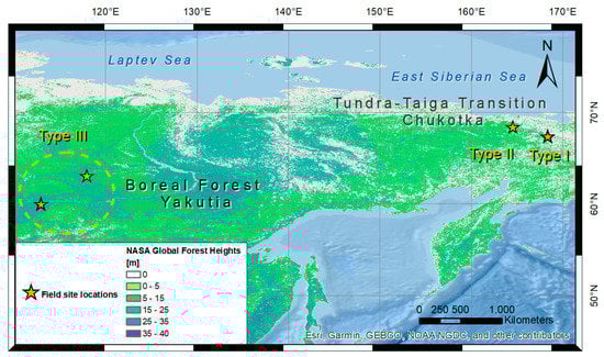
Figure 1.
Overview of the study region in NE Siberia and the selected forest sites. Type I: larch dominated, low density; Type II: larch dominated, ultra-high density; Type III: mixed tree species, high density.
2. Materials and Methods
2.1. Study Sites
Our study sites cover a bioclimatic gradient in north-eastern Russia (Figure 1) from extremely open larch forest with mean tree heights around 5 m in the vicinity of Lake Ilirney in central Chukotka (tundra–taiga ecotone, 67.36°N 168.32°E) to dense mixed tree species stands near Lake Khamra in south-western Yakutia (boreal forest biome, 59.99°N 112.98°E). We selected 10 plots with strong differences in stand structure that are representative of their region and classified them into three distinctive forest types (Types I, II, and III; see below) to help understand what kind of forests the methods are suitable for and to clarify their limitations. The representative plots for each forest type were chosen from a total set of 64 plots based on multiple criteria: the similarity of species composition within one type and the overall similarity of stand structure based on our field data including tree cover, density, and average vegetation heights; the availability and completeness of the UAV data and its quality in terms of light conditions during flight; and the exclusion of plots that did not produce good point clouds because flight height was too low above the canopy.
2.1.1. Type I: Open, Larch Dominated Stands
Type I sites (EN18001, 03, 12, 14, 26 and 27) are located in the proximity of Lake Ilirney. Larches (Larix cajanderi Mayr.) are the only tree forming vegetation. The herb layer consists of cotton-sedges (Eriophorum spp.), mosses, berries (e.g., Vaccinium uliginosum L., Vaccinium vitis-idaea L.), lichens, and dwarf- and low-shrub forming tree taxa such as dwarf birch (Betula nana L.), willow (Salix spp.), and infrequent Siberian dwarf pine (Pinus pumila (Pall.) Regel) and green alder (Alnus viridis (Chaix.) D.C.). The micro-topography of lowland sites is dominated by mounds of cotton-sedges, while better drained sites lack this species and hence show less micro-relief.
2.1.2. Type II: Dense, Larch Dominated Stands
Type II has a similar species composition to Type I, but is characterized by a higher tree density and cover. The site EN18030 (68.4055°N, 164.533°E) is located approximately 200 km west of Lake Ilirney and is characterized by extremely densely spaced narrow crowns. Field observations suggest that the area has experienced regular fire events, which have controlled the current stand structure. Outside the plot, but within the homogeneous stand, a few very large trees survived the fires.
2.1.3. Type III: Dense, Mixed Tree Species Stands
Type III includes sites EN18070, 80, and 83. They are located in central to south-western Yakutia and subject to different levels of disturbance. The stands are dominated by varying amounts of summergreen Dahurian larch trees (hybridization zone of Larix gmelinii (Rupr.) Rupr. and L. cajanderi), and evergreen Siberian pine (Pinus sibirica Du Tour) and Siberian spruce (Picea obovata Ledeb.), with occasional birch (Betula spp.) and Siberian fir (Abies sibirica Ledeb.). Alder and willow form large shrubs up to heights of 4 m. In contrast to the other plots, EN18070 was not meant to be homogeneous and representative for the region, but rather a transect itself reaching from a dense forest out into an open meadow. EN18080 has very open crowns, most likely due to a fire. EN18083 has much tree cover but also many dead trees lying on the forest floor, either windthrown or a result of fire disturbance.
2.2. Data Acquisition
The approximate plot locations were chosen beforehand based on landsat images. They represent dominant forest systems found in the region and are homogeneous in their spectral signal. In the field, the exact position was determined using the same criteria from the visual perspective. Two 30 m long tape measures were laid out along the main cardinal directions, intersecting in the plot center, marking the main axes of a circular area with a radius of 15 m (Figure 2). A minimum of 10 individuals of each tree and shrub species present were selected, for which we measured the stem diameter at breast height and at the base, identified damages (e.g., fire scars, wind damage, broken or dead terminal shoot, multi-stems), estimated the maximal and perpendicular to maximal crown diameter, tree height (or length: distance from the stem base to the top), crown start height, vitality in six categories, and cone quantity and quality. The position of the individuals was either recorded using a standard GPS device or noted as coordinates in the local grid. Additionally, we estimated the height of all trees > 20 cm in the four quadrants separated by the tape measures.
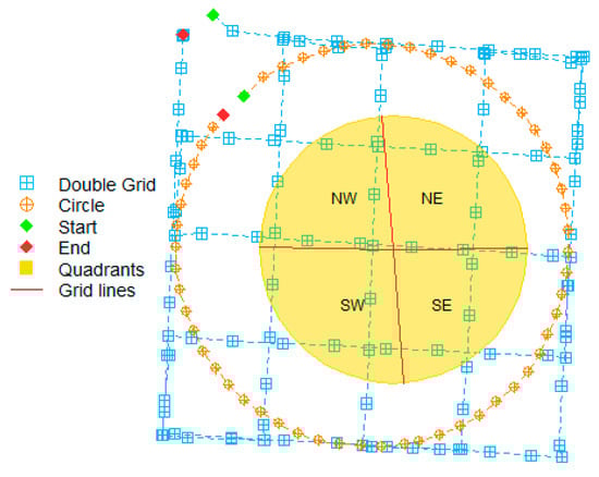
Figure 2.
Generic Unmanned Aerial Vehicle data acquisition and flight pattern consisting of a double grid (blue) and a circular mission (orange). The two 15 m long grid lines (red) divide the plot area into four quadrants of similar size (yellow).
We relied on a consumer grade DJI Phantom 4 quadcopter. The standard built-in camera of the type FC330 is a 12 megapixels RGB frame camera with a 94° field of view (FOV). It is tiltable on three axes via a gimbal and has a built in GPS/GLONASS receiver, automatically geo-tagging the images. The flight planning was executed with a free smartphone Android-application called Pix4Dcapture [42]. With no internet access in the field for over a month, we relied solely on the smartphone’s GPS position to manually set up the flight plans standing in the center of the plots. Each flight consisted of two successively flown flight patterns (Figure 2). We used a double grid pattern with 50 × 50 m grid extent and 30 m height above take-off elevation (ATOE). The camera was in near nadir position (facing 80° forward) to ensure the best image quality for the generation of orthomosaics. The sideways and frontal overlap was set to 85% and the flight speed to approximately 1 m/s. Additionally, a circular mission along a 25 m radius circle at 30 m ATOE acquired images with the camera pointing at the plot center at take-off elevation, which equals a camera angle of . We used this approach to gain a better image coverage of the crown sides and the ground below the forest canopy. The capture interval angle was set to 10° or lower, resulting in a minimum of 36 images in a full circle.
2.3. Ground Classification and the Derivation of Digital Elevation Models
The first step in our processing chain (Figure 3) was the reconstruction of dense point clouds in Agisoft PhotoScan Professional [43] using SfM and MVS techniques. In this manuscript, we refer to SfM and include the processing chain of SfM and MVS. We tuned the parameter settings to capture as much detail of the complex tree structures as possible. To achieve that, the alignment and dense cloud generation quality was set to highest and ultra-high. The depth filtering in the dense cloud generation was changed from the default to a mild filtering to preserve more detail. PhotoScan automatically integrated the GPS information of the images’ EXIF headers and geo-referenced all products.
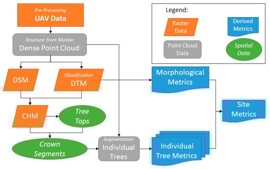
Figure 3.
Processing chain from pre-processed Unmanned Aerial Vehicle (UAV) data to site metrics. Abbreviations: UAV = Unmanned Aerial Vehicle, DSM = Digital Surface Model, DTM = Digital Terrain Model, CHM = Canopy Height Model.
To create a digital terrain model (DTM) the point cloud needed to be separated into two subsets, the first containing the higher vegetation and the second the remaining points representing the ground cover and lower vegetation (lying dead wood, shrubs, and the herb layer). For this step—called ground classification—a variety of morphological filters can be applied [44,45,46]. The Cloth Simulation Filter (CSF) after Zhang et al. [47] is a morphological filter that was developed for discrete return lidar point clouds and performs particularly well in conditions with highly variable micro-topography containing very few, or no, true ground points. It inverts the topography, or point cloud, and then simulates a piece of cloth being placed on top of the terrain, dropping into depressions and enclosing the high spots depending on the stiffness of its fabric. This simple design makes it very computationally effective (<3 s for point clouds with 30 million points). The filter is implemented in the R-package RCSF [48] and has three main parameters that should be adjusted. The scene parameter or rigidness adapts the algorithm to the overall site morphology and determines the first order stiffness of the cloth and can be 1 for flat scenes, 2 for minor relief, and 3 for steep slopes. The cloth resolution sets the cloth’s cell size. It should be set to a value that ensures flexibility for following the micro-topography, or low noise, while not being smaller than the inner diameter of the high vegetation bodies. The third parameter is the classification threshold that is the maximum distance between the cloth and a point to be classified as ground. All parameters used for the analysis of the sites are found in Table 1. The classes are stored in separate LAS files for convenient further analysis.

Table 1.
The applied parameters in the Cloth Simulation Filter ground classification are adjusted to the micro-topography and the quality of the point cloud.
The ground point clouds were rasterized on a 3 cm grid using a Triangular Irregular Network (TIN) algorithm, which performs a linear Delaunay interpolation within each triangle of the TIN. The next step was filtering the DTM with a local minimum moving window filter (15 × 15 px matrix) to shift the DTM below the herb layer and closer to the true ground (bare earth). This step was left out for sites that were characterized by low point densities and noisy ground to prevent pits from getting amplified (sites EN18030/80/83). Subsequently, a local mean filter of the same window size mitigates the effect of the micro-topography being forwarded to the CHM and closes potential pits from low outlier points. A digital surface model (DSM) is a raster interpolating between the highest points in each grid cell. Again, a 3 cm resolution grid is used to rasterize the full point cloud and the elevation value of the highest point in each cell is assigned as the new raster value. Single cells or small areas that do not contain any points (NA cells) get interpolated using TIN-interpolation (as for the DTM). For reconstructed DSMs with many apparent holes in the crowns, we used a different approach (sites EN18030/70): the interpolation during rasterization was disabled and the resulting holes in the DSM were filled with the DTM values of these cells. This prevents floating fragmented crowns belonging to multiple individuals without ground points below them from getting merged into a single large artificial crown by the interpolation.
The canopy height model (CHM) equals the difference between the DSM and the DTM (CHM = DSM–DTM), and thus normalizes the DSM to the ground. Each pixel represents the vegetation height above the ground. In preparation for the tree segmentation, two derived versions are calculated: an aggregated (resampling factor = 6, function = mean) CHM and a subsequently smoothed (3 × 3 px mean) CHM. The smoothing is an important step that prevents over-segmentation of crowns due to multiple spurious tree tops [49]. Stronger smoothing (5 × 5 px mean) can mitigate errors from fragmented crowns as present in sites EN18083 or EN18070. All raster products were clipped using a polygon mask created by fitting a convex hull around the XY projected points of the point cloud using the R package concaveman [50].
2.4. Individual Tree Detection and Crown Segmentation
Individual Tree Detection (ITD) and crown segmentation was done using the R-package ForestTools [51]. Mohan et al. [49] analyzed forest stands using canopy height models and found that the fixed window size of a tree detection local maximum filter (LMF) should be smaller for study sites with higher tree densities. The individual tree detection function vwf we used is based on Popescu et al. [52] and uses a dynamic circular moving window LMF. The window size is therefore different for every pixel as it calls a linear function that calculates the search window radius based on the pixel’s height. Thus, it considers the fact that large trees usually have larger crown diameters and prevents underestimating the number of small trees that otherwise would get incorporated into nearby larger trees. A pixel is defined as a tree top when no higher pixel is found in its search radius. Intuitively, the linear function should describe the allometric relationship between the tree’s height and its crown diameter. We experimented with various set-ups and found that generally a much narrower function works better to differentiate between closely spaced trees. This way, the search radius around a local maximum is smaller but the crown area could, as long as there is no secondary peak, still be indefinitely large. The implications of different formulae used in different kinds of forest structures are shown in Table 5. The functions used in this study are listed in Table 2.
Table 2.
The linear functions used for the individual tree detection determine the search radius r dependent on the pixel height h.
A marker-controlled inverse watershed segmentation (mcws) was conducted to identify the crown area corresponding to the detected tree tops. This method is similar to the watershed segmentation commonly used in hydrological analysis, where it separates the catchment basins of river networks [53]. The algorithm inverts the relief of the CHM, transforming protruding crowns into valleys. Taking the tree top markers as seed points, the gradient of each raster cell to its neighbors is calculated to determine the outline of the catchment or crown area. A minHeight parameter restricts the crown sides to a minimum height. Choosing a slightly larger value compensates for the enlargement of the crowns due to previous smoothing and aggregating. Every detected tree from now on has a unique identifier referred to as the TreeID.
2.5. Forest Stand Metric Derivation
The TreeID is passed on to a new field in the trees-only-LAS file used by a function from the rLiDAR package [54] called CrownMetrics. This function calculates a number of metrics, from which we only use two perpendicular crown diameters. It also filters out trees that do not contain multiple points. Tree height was calculated by finding the highest pixel value in the crown area of the unsmoothed DTM.
To validate the homogeneity of our plots within their surroundings, but still use the full extent of the point cloud, we divided each site into zones of different sizes. We digitized the grid lines and the plot center in PhotoScan and loaded the shape files, along with the orthophotos and CHMs, into ArcMap [55]. A 15 m buffer zone around the center point contoured the true plot area. The four ends of the grid lines were extended to the circle using the advanced editing toolbox. The features to polygon tool split the buffer polygon at its intercepts with the extended grid lines to create a polygon containing four quadrant polygon features. Starting from the plot center, six circular zones with successively increasing diameter (5 m intervals) were created and intersected with the point cloud area. The morphological site metrics and zonal statistics were calculated in those zones, as well as for the whole point cloud and the four field quadrants. The slope and the aspect of the DTM were calculated with the terrain function implemented in the raster package [56] and is based on Horn [57]. Trees that fall in each zone were sub-sampled and the SpatialPolygonsDataframe containing the crown areas was clipped for the calculation of the exact crown cover. Additionally, we calculated tree density as trees per hectare, mean tree height, crown, area and crown diameter plus their standard deviations.
2.6. Validation
To validate the “synthetic forest” it was necessary to assign the FieldID (observed trees) to the TreeID from the analysis (detected trees). As the field coordinates of the tree individuals had a high uncertainty and marked the position of the tree’s base, not its crown, we had to manually assign those points that were outside the corresponding crown area. We identified the crown polygons to which the field individuals corresponded and merged their data tables with functions from the R-package sp [58].
3. Results
3.1. Point Cloud Reconstruction and Individual Tree Detection
We successfully detected a total of 4719 trees and derived individual tree, stand structure, and site morphological metrics from 10 photogrammetric point clouds (Table 3; pre-processed point clouds are available for download at https://doi.pangaea.de/10.1594/PANGAEA.902259).
Table 3.
The shown metrics are calculated for the full point cloud extent.
The Type I sites have a mean tree density (ρ) of 551 trees per hectare (with a standard deviation (SD) of 155.39 ha−1, a minimum ρ of 492.67 ha−1 (EN18001), and a maximum ρ of 773.07 ha−1 (EN18027)), a mean tree height of 5.83 m (SD = 1.12 m), and a crown cover of 21.12% (SD = 3.43%). EN18030 as the only example of Type II has the highest tree density of 4597 ha−1, a mean tree height of 4.82 m, and a cover of 53%. Type III has a mean tree density of 1173 ha−1 (SD = 546.46 ha−1, minimum ρ = 801.07 ha−1 (EN18070), maximum ρ = 1800.33 ha−1 (EN18080)), a mean tree height of 12.53 m (SD = 6.45 m), and mean cover of 36% (SD = 5.29%). The mean crown area is highest in Type I (4.13 m2), slightly smaller in type III (3.61 m2), and lowest in Type II (1.15 m2).
3.2. Validation of Individual Tree Characteristics
We detected between 49% and 100% (mean = 74.8%, total detection rate of 67.1%) of the individual trees in each surveyed site. Typically, trees that the detection method failed to recognize were smaller than 2.5 m, but, depending on the stand structure, exceptions up to 12 m occurred as well (Table 4). Tall undetected trees stood either very close to or under a neighboring tree. Linear regressions of observed versus detected tree heights had a mean coefficient of determination (R2) value of 0.77 with the highest mean correlation in Type II ( N = 1), followed by Type III (, N = 4), and lowest in Type I (, N = 6). We removed an outlier in two cases (EN18012/14), where almost horizontally leaning trees were surveyed.
Table 4.
Validation results for individual tree metrics and stand structure for 10 field sites. Abbreviations: Nd = number detected, NO = number observed, H = tree height, CD = crown diameter. All heights, diameters, and corresponding root mean square error (RMSE) values are in meters.
The root mean square error (RMSE) varies for the three forest types with the highest mean RMSE in Type III (2.27 m), followed by Type I (1.135 m) and lowest in Type II (0.62 m). This indicates that the absolute errors are higher for taller trees. On average, the RMSE measures 18.46% of the mean tree height (RMSE%). Most sites show a cone shaped distribution of data points with stronger correlations for lower heights and higher variance with a tendency towards underestimation for greater heights (Figure 4). The detected heights of plot EN18083 dominantly overestimate the field heights. The regression model of EN18030 has a very pronounced interception point with the line of perfect correlation at approximately 5.8 m, marking a change from overestimation to underestimation.
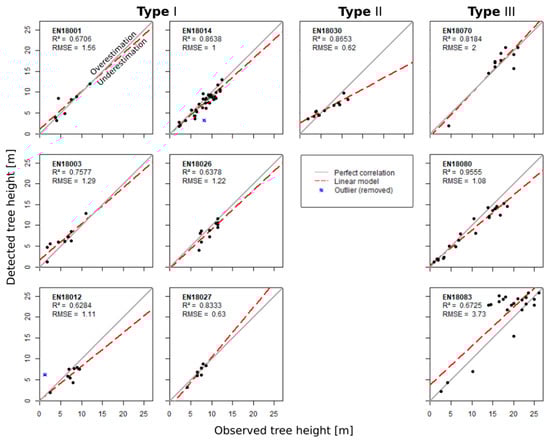
Figure 4.
The validation of detected versus observed tree heights for each of the 10 study sites with different forest structures sorted by forest type. The linear regressions (dashed red lines) show generally a good fit with regression lines running parallel to the bisecting line in combination with high coefficients of determination (R2) and low root mean square errors (RMSE). Type I: larch dominated, low density; Type II: larch dominated, ultra-high density; Type III: mixed tree species, high density.
The observed crown diameters are weakly correlated with the detected crown diameters (mean R2 = 0.46, mean RMSE = 0.67 m, mean RMSE% = 24.9%) and show a high inter-type variability (Figure 5). Type III has a very low mean R2 of 0.24, with no clear trend towards under- or over-estimation, whereas crown diameters of Type I sites are correlated more strongly than the average ( = 0.56).
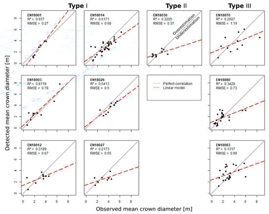
Figure 5.
Simple linear regressions (dashed red lines) of observed versus detected crown diameters. At many sites the estimated crown diameters of large trees were smaller than recorded during fieldwork, hence regression slopes are mostly <1 and coincide with low R2 values.
3.3. Validation of the Stand Structure
The observed height distributions of most sites show two distinctive peaks (Figure 6). The highest counts are always found in the first two height bins (0–1 and 1–2 m) and are separated from a symmetrical second peak that comprises taller trees by a prominent minimum. The early peaks are absent or greatly underrepresented in the single quadrant detected distributions, which is partly due to the low number of individuals. The field data of EN18030 has an asymmetrical single peak in the 2–4 m bins, while the detected distribution has its (also asymmetrical) peak at 4–6 m.
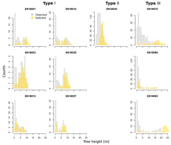
Figure 6.
Height distribution validation histograms (bin size = 1 m) of the corresponding plot area of 10 study sites ordered by forest type. Detected trees (yellow bars) show a good fit to observations (grey bars) for larger trees but fail to reflect the observed peak usually seen in the 0–2 m bins. Type I: larch dominated, low density; Type II: larch dominated, ultra-high density; Type III: mixed tree species, high density.
3.4. Zonal Homogeneity Analysis
To evaluate whether the chosen plot size (15 m radius circle) was an appropriate representation of the surrounding forest stand, we compared calculated site metrics for multiple successive growing areas (buffer zones). The tree density typically starts either very high or low in the first zone and slowly converges towards the point cloud mean (Figure 7). The first point of stability can give an estimate of the homogeneity of the stand.
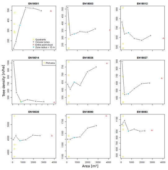
Figure 7.
Tree density values depend strongly on the size of the analyzed area. Black circles represent values for the circular buffer zones around the plot center with increasing radius (the smallest zone has a radius of 5 m ≈ 700 m2, the largest 30 m ≈ 2800 m2). In most cases the tree density converges at a radius of 15–20 m.
Tree density of sites EN18026/80 does not converge at all within their point cloud extent. EN18001/12/27 densities converge outside the 15 m buffer radius zone. The remaining sites EN18003/14/30/83 converge at smaller radii than 15 m. The mean tree height is spatially more stable and generally converges before the 15 m or even 10 m radius (Figure 8). The only exception is EN18001, where the mean tree height only stabilizes in the 20 m buffer zone.
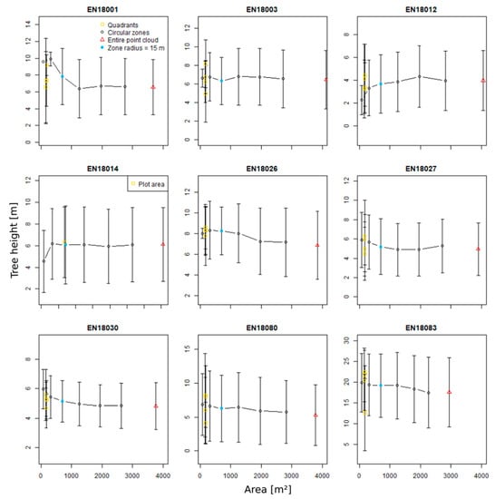
Figure 8.
Mean tree height is spatially more homogeneous that tree density and cover. Black error bars display the standard deviation.
Tree cover does not stabilize within the point cloud of sites EN18027/80/83, converges in the 15 m zone for sites EN18001/12/14/30, and in the 20 m zone of site EN18026 (Figure 9). The missing peak in the low heights, which was observed in the quadrant validation, is more pronounced in the detected height frequency distributions of the larger buffer zones. The distribution typically establishes the peak in the 0–15 m zone and reaches its final shape in the 0–20 m zone, with only minor changes occurring within larger radii.
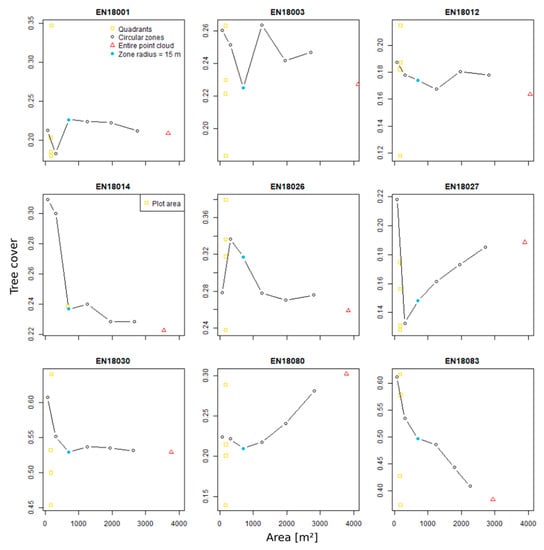
Figure 9.
Tree cover (fraction of ground covered by tree crown area) is the most heterogeneous of the studied metrics and often converges at large areas or not at all, indicating a heterogeneous stand structure.
4. Discussion
4.1. Methodology Applicability for Various Forest Structures
The task of detecting individual trees based on ultra-high resolution photogrammetric point clouds from the diverse types of forest stands encountered along the bioclimatic transect called for flexible, computationally efficient methods [59]. Therefore, we combined a cloth simulation filter ground-classification approach with a marker-controlled watershed crown segmentation algorithm, which delivered good estimates of tree position, height, and crown diameter. Despite the integration of both understory and dominant trees into our field survey (0.18–26 m), we successfully detect 67.1% of the validation trees. This rate is relatively low compared to other studies, which either deal with highly managed forest stands or do not consider small understory trees (e.g., [32,60,61]) and generally yield higher detection rates of 76% to 96%. Differences in stand complexity make it very difficult to compare detection methods across studies, as it has already been noted elsewhere [38]. Further, Hamraz et al. [39] point out that the inclusion of understory vegetation into the segmentation process is accompanied by an overall higher number of over-segmentation errors.
The comparison of field measured and detected crown diameters (mean R2 = 0.46, mean RMSE = 0.673 m, mean RMSE% = 24.9%) reveals bigger relative differences than the height validation (mean R2 = 0.77, mean RMSE = 1.135 m, mean RMSE% = 18.46%). Studies that have used similar methods report the same issue but with higher R2 values and larger root mean square errors. Popescu et al. [17] derived crown diameters for multiple sites in Virginia, USA using a small footprint lidar and report R2 values of 0.62 to 0.63 and RMSE values of 1.36 to 1.41 m. Panagiotidis et al. [30] conducted a UAV-based SfM study in mixed conifer stands in the Czech Republic and note a mean RMSE of 0.93 m and a mean R2 of 0.74. The weak correlation between observed and detected crown diameters could have its origin in the quality of the available field data, which are estimations instead of direct measurements and therefore have a decreasing precision with increasing heights. However, even though the vertical precision of the point clouds cannot be determined due to the lack of high precision control points, measuring the dimensions of ground features with known extend suggests that the horizontal errors (0.53 cm, SD = 1.15 cm) are much lower than the spatial resolution of the CHMs that were used for the analysis and can therefore be considered insignificant (Table A1). Hence, our crown diameter predictions are probably of similar high quality, given that the delineated crown contours are correct. This can be confirmed by visual assessment of the contours on an orthophoto. Another contribution to the observed differences could be the pooling of multiple crowns into one (omission errors).
Our field estimations are likely to have high uncertainty, especially for taller trees, as exemplified by the trumpet-shaped distribution seen in the tree height validation plots (Figure 4). The tendency for underestimating the height of taller trees could be explained by errors in the point cloud reconstruction of very thin tree tops. These errors have been identified and studied in detail by Andersen et al. [62].
The local maximum filter tree-detection algorithm works extremely well in open, simple structure forest stands, yet it produces more commission and omission errors for the dense stands of Type III, where smaller trees are more frequently overlapped by taller trees than in Type I sites. This is visible in the quadrant validation histograms, where a relatively smaller quantity of understory trees were detected (Figure 6), and in the height distribution of the whole point cloud (Figure A1). The prominent peak of small trees in the field data is largely underrepresented in the tree detection analysis, as small trees below a height of 2 m usually have narrow crowns and can hardly be distinguished from surrounding ground vegetation and shrubs. Their presence indicates a strong rejuvenation in recent years that could trigger a future densification of the forest stand, as has already been observed in other arctic regions [7,8]. The peak shift seen in the quadrant height distribution validation of site EN18030 accords with the behavior of the individual tree height validation regression and suggests either an underestimation of the true height in the field data or an overestimation of true heights from the analyzed point cloud.
The detection of small trees is a general limitation of current tree detection algorithms. While the tree recruits in most biomes grow fast and can therefore be detected earlier by such methods, under the harsh conditions of the treeline ecotone, recruits can survive under the canopy of a dominant tree for many years with nearly no growth [63]. However, they play an important role in the tundra–taiga ecotone, as they are an indicator of the outcome of climate warming [8,9]. Integrating spectral classification metrics into the segmentation analysis could help distinguish small trees from surrounding shrubs of the same height or even to determine the tree species in mixed species stands [34]. Higher point densities in critical areas like the lower crowns and smaller individuals could be achieved by additional imagery with shallower capture angles or even ground-based acquisitions and contribute to better segmentation results. Such data was already collected but could not yet be integrated into the analysis.
Our representativeness evaluation gives first insights into the relationship between the calculated stand metrics and the minimal required plot size for representative forest inventories in treeline ecotones. We find three types of zonal metric convergence behaviors: (1) plots that show stable tree density values inside the 15 m radius can be called representative (EN18003/14/30/83), (2) convergence outside the 15 m radius implies homogeneity of the stand at broader scales, for which a bigger plot radius is necessary (EN18001/12/27), and (3) no convergence within the full point cloud extent, indicating an unrepresentative plot choice and a heterogeneous stand structure surrounding the plot center (EN18026/80). Most calculated metrics converge towards stability at a plot size of 20 m, indicating that our field data (15 m radius plot size) might not be fully representative of the surrounding stand. Some sites do not show homogeneity at the complete point cloud extent and are thus considered to be heterogeneous. These findings suggest that the plot size should be adapted to the stand structure in order to deduce representative forest inventories. Yet most studies with similar approaches, albeit none of them in a treeline ecotone, have used smaller validation plot sizes (Bohlin et al. [32] used a 10 m radius, Li et al. [21] a 12.62 m radius, Popescu et al. [17] a 7.32 m radius, and Panagiotidis et al. [30] a 25 × 25 m rectangular plot). To optimize future survey efforts, our information could be used for helping to choose the required validation plot size and UAV survey dimensions.
In summary, the discussed issues underline the strong need for new, point cloud-based segmentation methods to fully exploit the potential of 3D photogrammetric point clouds. These algorithms should be capable of detecting subordinate individuals as well as small trees and allow the correct segmentation of overlapping or intersecting crowns. Currently available point cloud-based segmentation algorithms are still too inefficient for high-resolution photogrammetric point clouds (for example, the computation time of the algorithm by Li et al. [21] exponentially rises with the point density [38]). Some promising novel techniques initially segment the normalized point cloud into vegetation stories to subsequently run an individual tree detection within those vertical levels [39,40], or add an additional step after the 2D segmentation to delineate potential subordinate trees under the dominant crown [41]. Both of these methods could have great potential for the segmentation of understory individuals.
4.2. Challenges in the Tree Segmentation Based on Canopy Height Models
The CHM-based individual tree detection (ITD) and crown segmentation is very simple to set up and computationally efficient, but has some major limitations that arise from the dimensionality of the analysis. Some issues are integral to this method, while others can be controlled or mitigated by the right parameter choice. Typical types of errors are over-segmentation (commission errors), under-segmentation (omission errors), and the underestimation of the tree height (Table 5).
Table 5.
Types of issues that are associated with the use of a local maximum filter individual tree detection in combination with a watershed crown segmentation.
Over-segmentation occurs when an area is segmented into more individuals than exist. Under-segmentation occurs when fewer trees than exist are detected, or are not detected at all. Controlling parameters are the linear function and minimal height used in the ITD and the smoothing factor used on the CHM. Generally, these parameters should be optimized to the stand structure based on a priori knowledge and steady re-adjustment (this is only possible due to the fast computation times). Individuals will create errors when differing in shape from the dominant structure the analysis was optimized for. Therefore, stands with a very homogeneous structure will perform better than stands that show high structural complexity.
Identified inevitable errors comprise the omission of subordinate trees, whose tops are hidden below an overlapping crown, underestimation of the height of leaning trees (if individual tree point clouds contain absolutely no ground points the calculation of the Euclidean distance between the highest and lowest point solves this problem), trees whose tops have not been fully reconstructed (mostly dead, leafless, or very thin tops), and small shrub-forming trees. The latter have crowns that reach down to the ground and get partially classified as ground points. Other errors we observed result from exceptional individuals, which are often found in unmanaged forests and the discussed parameters could not be optimized for.
Four important examples illustrated in Figure 10 are:
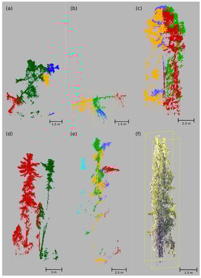
Figure 10.
Examples of commission (a–c,e) and omission (d,f) errors. (a–e) are colored by ID, (f) by RGB values.
5. Conclusions
The analysis of high-resolution photogrammetric point clouds resulted in detailed forest metrics along the studied transect ranging from the open larch forests of the tundra–taiga transition zone in NE Chukotka to disturbed, dense, mixed tree species forest in SW Yakutia. These metrics can be used to facilitate models and upscaling approaches to study regional vegetation dynamics such as the treeline response to global warming in NE Siberian forest biomes. Our detection approach is based on canopy height models. The individual tree detection using a variable window-size local maximum filter and subsequent crown delineation using a marker-controlled inverse watershed segmentation work efficiently and were adaptable to the encountered types of forest structures. The overall detection rate of 67.1% can be attributed to the incorporation of understory trees into the validation process. We found that omission and commission errors are more frequent in complex forests stands, in which dominant trees overlap the understory and multiple tree species with varying crown structures make it more complicated to adapt the tree detection algorithm parameters. Our detected tree heights correlate strongly with field observations, while the crown diameters show higher absolute errors, probably caused by imprecise field measurements. Comprehensive fieldwork is still crucial to obtain an estimate of the true tree height distribution, as small trees (height <2 m) typically do not get identified in the CHM-based analysis, but are very important for the recruitment and observed densification of forest tundra stands. To help improve future fieldwork routines, the correct validation plot size needs to be determined and segmentation errors can be mitigated by optimizing the analysis parameters. Based on our results, we identified a strong need for computationally efficient individual tree detection algorithms and clear guidelines and best-practice studies to use them. With these, one could use the full potential of high-resolution photogrammetric point clouds and focus on scientific questions related the detection of understory and subordinate trees.
Author Contributions
F.B. and S.K. designed the study. S.K., F.B., U.H., E.S.Z. and L.A.P. conducted fieldwork. F.B. processed and analyzed the data and wrote a first version of the paper that all co-authors commented on.
Funding
The positions of Stefan Kruse and Ulrike Herzschuh were funded by the ERC consolidator grant Glacial Legacy of Ulrike Herzschuh (grant no. 772852).
Acknowledgments
We thank our Russian and German colleagues from the joint Russian–German expedition 2018 for support in the field. Special thanks to Lena A. Ushnitskaya, Luise Schulte, and Iuliia A. Shevtsova for their help in sampling and tree measurements. Guido Grosse and Thomas Laepple provided us with computational resources for the point cloud reconstruction. We thank Cathy Jenks for proofreading and improving the paper.
Conflicts of Interest
The authors declare no conflict of interest.
Appendix A

Figure A1.
Height distributions of all detected trees within the point cloud extents.
Appendix B
Table A1.
The horizontal accuracy of the point cloud was tested by measuring ground control point panels with known dimensions of 21 × 29.7 cm. The test shows that the mean XY difference (0.52 cm, SD = 1.15 cm) is much lower than the spatial resolution of the CHMs used for the analysis (3 cm). Abbreviations: No = Number, W = width, H = height, Wdiff = W–21 cm, Hdiff = H–29.7 cm, MeanDiff = mean difference, SD = standard deviation.
| Site | No | W (cm) | H (cm) | Wdiff (cm) | Hdiff (cm) |
|---|---|---|---|---|---|
| EN18001 | 1 | 23.9 | 29.3 | −0.4 | 2.9 |
| EN18001 | 2 | 21.2 | 31.2 | 1.5 | 0.2 |
| EN18001 | 3 | 21.9 | 28.8 | −0.9 | 0.9 |
| EN18003 | 1 | 22.4 | 30.4 | 0.7 | 1.4 |
| EN18003 | 2 | 20.9 | 30.1 | 0.4 | −0.1 |
| EN18003 | 3 | 23 | 30.4 | 0.7 | 2 |
| EN18012 | 1 | 20.3 | 30.4 | 0.7 | −0.7 |
| EN18012 | 2 | 21.5 | 30.4 | 0.7 | 0.5 |
| EN18012 | 3 | 20.9 | 29.2 | −0.5 | −0.1 |
| EN18014 | 1 | 22.5 | 30.3 | 0.6 | 1.5 |
| EN18014 | 2 | 21.8 | 30.7 | 1 | 0.8 |
| EN18014 | 3 | 22 | 30.9 | 1.2 | 1 |
| EN18026 | 1 | 21.4 | 27.7 | −2 | 0.4 |
| EN18026 | 2 | 21.1 | 30.3 | 0.6 | 0.1 |
| EN18026 | 3 | 21.4 | 28.7 | −1 | 0.4 |
| EN18027 | 1 | 21 | 29 | −0.7 | 0 |
| EN18027 | 2 | 23.3 | 29.5 | −0.2 | 2.3 |
| EN18027 | 3 | 21.2 | 31.2 | 1.5 | 0.2 |
| EN18030 | 1 | 20.2 | 29.6 | −0.1 | −0.8 |
| EN18030 | 2 | 20.2 | 29.7 | 0 | −0.8 |
| EN18030 | 3 | 20.7 | 30.6 | 0.9 | −0.3 |
| EN18070 | 1 | 22.6 | 30.7 | 1 | 1.6 |
| EN18070 | 2 | 23.2 | 32.1 | 2.4 | 2.2 |
| EN18070 | 3 | 21.2 | 29.7 | 0 | 0.2 |
| EN18080 | 1 | 21.3 | 28.6 | −1.1 | 0.3 |
| EN18080 | 2 | 22.6 | 30.4 | 0.7 | 1.6 |
| EN18080 | 3 | 20.4 | 30.8 | 1.1 | −0.6 |
| EN18083 | 1 | 22.2 | 31.2 | 1.5 | 1.2 |
| EN18083 | 2 | 23 | 26 | −3.7 | 2 |
| EN18083 | 3 | 22.4 | 32.5 | 2.8 | 1.4 |
| MeanDiff | SD | ||||
| 0.51833333 | 1.15057836 |
References
- Holland, M.M.; Bitz, C.M. Polar amplification of climate change in coupled models. Clim. Dyn. 2003, 21, 221–232. [Google Scholar] [CrossRef]
- Bekryaev, R.V.; Polyakov, I.V.; Alexeev, V.A. Role of polar amplification in long-term surface air temperature variations and modern arctic warming. J. Clim. 2010, 23, 3888–3906. [Google Scholar] [CrossRef]
- Snyder, P.K.; Delire, C.; Foley, J.A. Evaluating the influence of different vegetation biomes on the global climate. Clim. Dyn. 2004, 23, 279–302. [Google Scholar] [CrossRef]
- Bonan, G.B. Forests and Climate Change: Forcings, Feedbacks, and the Climate. Science 2008, 320, 1444–1449. [Google Scholar] [CrossRef] [PubMed]
- Ranson, K.J.; Montesano, P.M.; Nelson, R. Object-based mapping of the circumpolar taiga-tundra ecotone with MODIS tree cover. Remote Sens. Environ. 2011, 115, 3670–3680. [Google Scholar] [CrossRef]
- Kravtsova, V.I.; Tutubalina, O.V.; Hofgaard, A. Aerospace Mapping of the Status and Position of Northern Forest Limit. Geogr. Environ. Sustain. 2012, 5, 28–47. [Google Scholar] [CrossRef]
- Frost, G.V.; Epstein, H.E. Tall shrub and tree expansion in Siberian tundra ecotones since the 1960s. Glob. Chang. Biol. 2014, 20, 1264–1277. [Google Scholar] [CrossRef]
- Wieczorek, M.; Kruse, S.; Epp, L.S.; Kolmogorov, A.; Nikolaev, A.N.; Heinrich, I.; Jeltsch, F.; Pestryakova, L.A.; Zibulski, R.; Herzschuh, U. Dissimilar responses of larch stands in northern Siberia to increasing temperatures—A field and simulation based study. Ecology 2017, 98, 2343–2355. [Google Scholar] [CrossRef]
- Kruse, S.; Wieczorek, M.; Jeltsch, F.; Herzschuh, U. Treeline dynamics in Siberia under changing climates as inferred from an individual-based model for Larix. Ecol. Modell. 2016, 338, 101–121. [Google Scholar] [CrossRef]
- Kruse, S.; Gerdes, A.; Kath, N.J.; Epp, L.S.; Stoof-Leichsenring, K.R.; Pestryakova, L.A.; Herzschuh, U. Dispersal distances and migration rates at the arctic treeline in Siberia; a genetic and simulation based study. Biogeosciences 2019, 16, 1211–1224. [Google Scholar] [CrossRef]
- Grace, J.; Berninger, F.; Nagy, L. Impacts of climate change on the tree line. Ann. Bot. 2002, 90, 537–544. [Google Scholar] [CrossRef] [PubMed]
- Ranson, K.J.; Sun, G.; Kharuk, V.I.; Kovacs, K. Assessing tundra-taiga boundary with multi-sensor satellite data. Remote Sens. Environ. 2004, 93, 283–295. [Google Scholar] [CrossRef]
- Mathisen, I.E.; Mikheeva, A.; Tutubalina, O.V.; Aune, S.; Hofgaard, A. Fifty years of tree line change in the Khibiny Mountains, Russia: Advantages of combined remote sensing and dendroecological approaches. Appl. Veg. Sci. 2014, 17, 6–16. [Google Scholar] [CrossRef]
- Montesano, P.M.; Neigh, C.S.R.; Sexton, J.; Feng, M.; Channan, S.; Ranson, K.J.; Townshend, J.R. Calibration and Validation of Landsat Tree Cover in the Taiga-Tundra Ecotone. Remote Sens. 2016, 8, 551. [Google Scholar] [CrossRef]
- Mikheeva, A.I.; Tutubalina, O.V.; Zimin, M.V.; Golubeva, E.I. A Subpixel Classification of Multispectral Satellite Imagery for Interpetation of Tundra-Taiga Ecotone Vegetation (Case Study on Tuliok River Valley, Khibiny, Russia). Izv. Atmos. Ocean. Phys. 2017, 53, 1164–1173. [Google Scholar] [CrossRef]
- Nilsson, M. Estimation of tree heights and stand volume using an airborne lidar system. Remote Sens. Environ. 1996, 56, 1–7. [Google Scholar] [CrossRef]
- Popescu, S.C.; Wynne, R.H.; Nelson, R.F. Measuring individual tree crown diameter with lidar and assessing its influence on estimating forest volume and biomass. Can. J. Remote Sens. 2003, 29, 564–577. [Google Scholar] [CrossRef]
- Morsdorf, F.; Meier, E.; Kötz, B.; Itten, K.I.; Dobbertin, M.; Allgöwer, B. LIDAR-based geometric reconstruction of boreal type forest stands at single tree level for forest and wildland fire management. Remote Sens. Environ. 2004, 92, 353–362. [Google Scholar] [CrossRef]
- Rees, W.G. Characterisation of Arctic treelines by LiDAR and multispectral imagery. Polar Rec. (Gr. Br.) 2007, 43, 345–352. [Google Scholar] [CrossRef]
- Edson, C.; Wing, M.G. Airborne light detection and ranging (LiDAR) for individual tree stem location, height, and biomass measurements. Remote Sens. 2011, 3, 2494–2528. [Google Scholar] [CrossRef]
- Li, W.; Guo, Q.; Jakubowski, M.K.; Kelly, M. A New Method for Segmenting Individual Trees from the Lidar Point Cloud. Photogramm. Eng. Remote Sens. 2012, 78, 75–84. [Google Scholar] [CrossRef]
- Plowright, A. Extracting Trees in An Urban Environment Using Airborne LiDAR. Doctoral Dissertation, University of British Columbia Library, Vancouver, BC, Canada, 2015. [Google Scholar]
- Westoby, M.J.; Brasington, J.; Glasser, N.F.; Hambrey, M.J.; Reynolds, J.M. “Structure-from-Motion” photogrammetry: A low-cost, effective tool for geoscience applications. Geomorphology 2012, 179, 300–314. [Google Scholar] [CrossRef]
- Alonzo, M.; Bookhagen, B.; McFadden, J.P.; Sun, A.; Roberts, D.A. Mapping urban forest leaf area index with airborne lidar using penetration metrics and allometry. Remote Sens. Environ. 2015, 162, 141–153. [Google Scholar] [CrossRef]
- Baguskas, S.A.; Peterson, S.H.; Bookhagen, B.; Still, C.J. Evaluating spatial patterns of drought-induced tree mortality in a coastal California pine forest. For. Ecol. Manag. 2014, 315, 43–53. [Google Scholar] [CrossRef]
- Mathews, A.J.; Jensen, J.L.R. Visualizing and quantifying vineyard canopy LAI using an unmanned aerial vehicle (UAV) collected high density structure from motion point cloud. Remote Sens. 2013, 5, 2164–2183. [Google Scholar] [CrossRef]
- Dandois, J.P.; Ellis, E.C. High spatial resolution three-dimensional mapping of vegetation spectral dynamics using computer vision. Remote Sens. Environ. 2013, 136, 259–276. [Google Scholar] [CrossRef]
- Fraser, R.H.; Olthof, I.; Lantz, T.C.; Schmitt, C. UAV photogrammetry for mapping vegetation in the low-Arctic. Arct. Sci. 2016, 2, 79–102. [Google Scholar] [CrossRef]
- Jensen, J.L.R.; Mathews, A.J. Assessment of image-based point cloud products to generate a bare earth surface and estimate canopy heights in a woodland ecosystem. Remote Sens. 2016, 8, 50. [Google Scholar] [CrossRef]
- Panagiotidis, D.; Abdollahnejad, A.; Surový, P.; Chiteculo, V. Determining tree height and crown diameter from high-resolution UAV imagery. Int. J. Remote Sens. 2017, 38, 2392–2410. [Google Scholar] [CrossRef]
- Frey, J.; Kovach, K.; Stemmler, S.; Koch, B. UAV Photogrammetry of Forests as a Vulnerable Process. A Sensitivity Analysis for a Structure from Motion RGB-Image Pipeline. Remote Sens. 2018, 10, 912. [Google Scholar] [CrossRef]
- Bohlin, J.; Wallerman, J.; Fransson, J.E.S. Forest variable estimation using photogrammetric matching of digital aerial images in combination with a high-resolution DEM. Scand. J. For. Res. 2012, 27, 692–699. [Google Scholar] [CrossRef]
- Fritz, A.; Kattenborn, T.; Koch, B. UAV-based photogrammetric point clouds—Tree stem Mapping in open stands in Comparison to Terrestrial Laser Scanner Point Clouds. Int. Arch. Photogramm. Remote Sens. Spat. Inf. Sci. ISPRS Arch. 2013, XL-1/W2, 141–146. [Google Scholar] [CrossRef]
- St-Onge, B.; Audet, F.A.; Bégin, J. Characterizing the height structure and composition of a boreal forest using an individual tree crown approach applied to photogrammetric point clouds. Forests 2015, 6, 3899–3922. [Google Scholar] [CrossRef]
- Ota, T.; Ogawa, M.; Shimizu, K.; Kajisa, T.; Mizoue, N.; Yoshida, S.; Takao, G.; Hirata, Y.; Furuya, N.; Sano, T.; et al. Aboveground biomass estimation using structure from motion approach with aerial photographs in a seasonal tropical forest. Forests 2015, 6, 3882–3898. [Google Scholar] [CrossRef]
- Ferraz, A.; Saatchi, S.; Mallet, C.; Meyer, V. Lidar detection of individual tree size in tropical forests. Remote Sens. Environ. 2016, 183, 318–333. [Google Scholar] [CrossRef]
- Ayrey, E.; Fraver, S.; Kershaw, J.A.; Kenefic, L.S.; Hayes, D.; Weiskittel, A.R.; Roth, B.E. Layer Stacking: A Novel Algorithm for Individual Forest Tree Segmentation from LiDAR Point Clouds. Can. J. Remote Sens. 2017, 43, 16–27. [Google Scholar] [CrossRef]
- Pirotti, F.; Kobal, M.; Roussel, J.R. A Comparison of Tree Segmentation Methods Using Very High Density Airborne Laser Scanner Data. Int. Arch. Photogramm. Remote Sens. Spat. Inf. Sci. 2017, XLII-2/W7, 285–290. [Google Scholar] [CrossRef]
- Hamraz, H.; Contreras, M.A.; Zhang, J. Vertical stratification of forest canopy for segmentation of understory trees within small-footprint airborne LiDAR point clouds. ISPRS J. Photogramm. Remote Sens. 2017, 130, 385–392. [Google Scholar] [CrossRef]
- Hamraz, H.; Contreras, M.A.; Zhang, J. Forest understory trees can be segmented accurately within sufficiently dense airborne laser scanning point clouds. Sci. Rep. 2017, 7, 1–9. [Google Scholar] [CrossRef]
- Harikumar, A.; Bovolo, F.; Bruzzone, L. A local projection-based approach to individual tree detection and 3-d crown delineation in multistoried coniferous forests using high-density airborne LiDAR data. IEEE Trans. Geosci. Remote Sens. 2019, 57, 1168–1182. [Google Scholar] [CrossRef]
- Pix4D SA Pix4Dcapture, App Version 4.3.0. 2018. Available online: https://www.pix4d.com/product/pix4dcapture (accessed on 15 May 2019).
- Agisoft LLC. Agisoft PhotoScan Professional, Version 1.4.3; Agisoft LLC: St. Petersburg, Russia, 2018.
- Kobler, A.; Pfeifer, N.; Ogrinc, P.; Todorovski, L.; Oštir, K.; Džeroski, S. Repetitive interpolation: A robust algorithm for DTM generation from Aerial Laser Scanner Data in forested terrain. Remote Sens. Environ. 2007, 108, 9–23. [Google Scholar] [CrossRef]
- Chen, Q.; Gong, P.; Baldocchi, D.; Xie, G. Filtering Airborne Laser Scanning Data with Morphological Methods. Photogramm. Eng. Remote Sens. 2013, 73, 175–185. [Google Scholar] [CrossRef]
- Pingel, T.J.; Clarke, K.C.; McBride, W.A. An improved simple morphological filter for the terrain classification of airborne LIDAR data. ISPRS J. Photogramm. Remote Sens. 2013, 77, 21–30. [Google Scholar] [CrossRef]
- Zhang, W.; Qi, J.; Wan, P.; Wang, H.; Xie, D.; Wang, X.; Yan, G. An easy-to-use airborne LiDAR data filtering method based on cloth simulation. Remote Sens. 2016, 8, 501. [Google Scholar] [CrossRef]
- Roussel, J.-R.; Qi, J. RCSF: Airborne LiDAR Filtering Method Based on Cloth Simulation. R Package Version 1.0.1. 2018. Available online: https://CRAN.R-project.org/package=RCSF (accessed on 17 May 2019).
- Mohan, M.; Silva, C.A.; Klauberg, C.; Jat, P.; Catts, G.; Cardil, A.; Hudak, A.T.; Dia, M. Individual tree detection from unmanned aerial vehicle (UAV) derived canopy height model in an open canopy mixed conifer forest. Forests 2017, 8, 340. [Google Scholar] [CrossRef]
- Gombin, J.; Vaidyanathan, R.; Agafonkin, V. Concaveman: A Very Fast 2D Concave Hull Algorithm. R Package Version 1.0.0. 2017. Available online: https://CRAN.R-project.org/package=concaveman (accessed on 17 May 2019).
- Plowright, A. ForestTools: Analyzing Remotely Sensed Forest Data. R Package Version 0.2.0. 2018. Available online: https://github.com/AndyPL22/ForestTools (accessed on 17 May 2019).
- Popescu, S.C.; Wynne, R.H. Seeing the trees in the forest: Using lidar and multispectral data fusion with local filtering and variable window size for estimating tree height. Photogramm. Eng. Remote Sens. 2004, 70, 589–604. [Google Scholar] [CrossRef]
- Meyer, F.; Beucher, S. Morphological Segmentation. J. Vis. Commun. Image Represent. 1990, 1, 21–46. [Google Scholar] [CrossRef]
- Silva, C.A.; Crookston, N.L.; Hudak, A.T.; Vierling, L.A.; Klauberg, C.; Cardil, A. rLiDAR: LiDAR Data Processing and Visualization. R Package Version 0.1.1. 2017. Available online: https://CRAN.R-project.org/package=rLiDAR (accessed on 17 May 2019).
- ESRI. ArcGIS Desktop, version 10.5.1; ESRI: Redlands, CA, USA, 2019.
- Hijmans, R.J. raster: Geographic Data Analysis and Modeling. R Package Version 2.8-19. 2019. Available online: https://CRAN.R-project.org/package=raster (accessed on 17 May 2019).
- Horn, B.K.P. Hill Shading and the Reflectance Map. Proc. IEEE 1981, 69, 14–47. [Google Scholar] [CrossRef]
- Pebesma, E.J.; Bivand, R.S. Classes and Methods for Spatial Data in R. R News 5 (2). 2005. Available online: https://cran.r-project.org/doc/Rnews (accessed on 17 May 2019).
- Zhen, Z.; Quackenbush, L.J.; Zhang, L. Trends in automatic individual tree crown detection and delineation-evolution of LiDAR data. Remote Sens. 2016, 8, 333. [Google Scholar] [CrossRef]
- Silva, C.A.; Hudak, A.T.; Vierling, L.A.; Loudermilk, E.L.; O’Brien, J.J.; Hiers, J.K.; Jack, S.B.; Gonzalez-Benecke, C.; Lee, H.; Falkowski, M.J.; et al. Imputation of Individual Longleaf Pine (Pinus palustris Mill.) Tree Attributes from Field and LiDAR Data. Can. J. Remote Sens. 2016, 42, 554–573. [Google Scholar] [CrossRef]
- Wallace, L.; Lucieer, A.; Malenovskỳ, Z.; Turner, D.; Vopěnka, P. Assessment of forest structure using two UAV techniques: A comparison of airborne laser scanning and structure from motion (SfM) point clouds. Forests 2016, 7, 62. [Google Scholar] [CrossRef]
- Andersen, H.E.; Reutebuch, S.E.; McGaughey, R.J. A rigorous assessment of tree height measurements obtained using airborne lidar and conventional field methods. Can. J. Remote Sens. 2006, 32, 355–366. [Google Scholar] [CrossRef]
- Osawa, A.; Zyryanova, O.A.; Matsuura, Y.; Kajimoto, T.; Wein, R.W. Permafrost Ecosystems: Siberian Larch Forests; Springer: Berlin/Heidelberg, Germany, 2010; ISBN 9781402096921. [Google Scholar]
© 2019 by the authors. Licensee MDPI, Basel, Switzerland. This article is an open access article distributed under the terms and conditions of the Creative Commons Attribution (CC BY) license (http://creativecommons.org/licenses/by/4.0/).