Large-Area, High Spatial Resolution Land Cover Mapping Using Random Forests, GEOBIA, and NAIP Orthophotography: Findings and Recommendations

Abstract

Despite the need for quality land cover information, large-area, high spatial resolution land cover mapping has proven to be a difficult task for a variety of reasons including large data volumes, complexity of developing training and validation datasets, data availability, and heterogeneity in data and landscape conditions. We investigate the use of geographic object-based image analysis (GEOBIA), random forest (RF) machine learning, and National Agriculture Imagery Program (NAIP) orthophotography for mapping general land cover across the entire state of West Virginia, USA, an area of roughly 62,000 km². We obtained an overall accuracy of 96.7% and a Kappa statistic of 0.886 using a combination of NAIP orthophotography and ancillary data. Despite the high overall classification accuracy, some classes were difficult to differentiate, as highlight by the low user’s and producer’s accuracies for the barren, impervious, and mixed developed classes. In contrast, forest, low vegetation, and water were generally mapped with accuracy. The inclusion of ancillary data and first- and second-order textural measures generally improved classification accuracy whereas band indices and object geometric measures were less valuable. Including super-object attributes improved the classification slightly; however, this increased the computational time and complexity. From the findings of this research and previous studies, recommendations are provided for mapping large spatial extents.

1. Introduction

Supervised classification of land cover at a high spatial resolution (1–5 m) over large areas can be challenging due to large data volumes, computational load, processing time, complexity of developing training and validation datasets, data availability, and heterogeneity in data and landscape conditions [1,2,3,4,5,6]. High spatial resolution land cover datasets are not commonly available over large spatial extents, such as entire continents or countries, in contrast to moderate spatial resolution land cover data such as the National Land Cover Database (NLCD) in the United States [7] or the Coordination of Information on the Environment (CORINE) Land Cover data in Europe [8]. Land cover and land use data are often cited as important information sources for monitoring and modeling ecological systems [9], biodiversity [10], landscape alterations [11], and climate change [12], highlighting the need for continued research on supervised image classification methods applicable to large datasets and for use at more local scales.

Some high resolution and large-area mapping projects have already been undertaken. For example, Basu et al. [1] mapped the extent of tree canopy cover across the entire state of California using 1 m aerial imagery and suggested that the proposed method could be applied to the entirety of the contiguous United States (CONUS). O’Neil-Dunne et al. [4] used geographic object-based image analysis (GEOBIA) methods and a variety of high spatial resolution datasets to map urban and suburban tree canopy cover in more than 70 cities and counties in the United States. In contrast, high spatial resolution products that differentiate multiple classes are rarer; however, there are exceptions. For example, the Chesapeake Conservancy and partners produced a 1 m land cover dataset for all counties that intersect the Chesapeake Bay drainage basin, an area of approximately 250,000 km² [13]. These data are currently being used to train a deep neural network model implemented by Microsoft Azure AI [14].

The goal of this paper is to highlight findings and provide recommendations for high spatial resolution, large-area land cover mapping. The results pertain to a land cover mapping project covering the full extent of the state of West Virginia, USA, an area of roughly 62,000 km². Using a combination of random forests (RF) machine learning and GEOBIA, a 1 m resolution, six-class land cover classification is generated. The input data are four-band, color infrared (CIR) orthophotography from the National Agriculture Imagery Program (NAIP) and ancillary data. We investigate the impact of training sample size and predictor variable feature selection. Additionally, we experiment with including measures derived from super-objects, or larger objects that contain the object being classified, and measures of object geometry and texture, or measures of spatial variability. The following findings and recommendations are discussed:

• How is classification accuracy of RF impacted by training data sample size and feature selection over a large spatial extent?
• Does incorporating GEOBIA super-object information improve classification accuracy?
• Does the addition of geometric measures, first-order textural measures, or second-order textural measures improve classification accuracy? If so, what variables are most important?
• Does the incorporation of ancillary data improve classification accuracy? If so, what variables are most important?
• What practical techniques are useful for processing this large data volume?

1.1. Machine Learning and Training Data

The RF algorithm is used to perform all land cover classification experiments in this study. This algorithm is a nonparametric machine learning method based upon an ensemble of decision trees (DTs) [15,16,17]. DTs use recursive splitting rules to divide the input data into more homogenous groups, a process that produces a set of decision rules based on the input predictor variables or image bands that can be used to classify new data [18]. RF expands upon single DTs by producing multiple trees as an ensemble. Each tree in the ensemble is generated using a subset of the training data produced using bagging, or random sampling with replacement. Each tree is also provided with a random subset of the predictor variables. Because each tree does not use the entire training set, the withheld samples from each tree, known as out-of-bag (OOB) samples, can be used to assess model performance [15,16,17]. RF has been applied to a variety of image classification tasks including mapping urban land cover [19,20], surface mines [21], agriculture [17], and general land cover [3,6,16,22]. Although they caution against using RF for all classification tasks, Lawrence et al. [23] found that it provided the highest overall accuracy when averaged across a variety of experiments when compared against boosted DTs, support vector machines (SVMs), and other methods. Ma et al. [24] suggested that RF generally provides the best performance for the classification of image objects when using GEOBIA methods. Its many strengths include ease of optimization, ability to assess predictor variable importance, robustness to noisy input data and mislabeled training samples, and the ability to accept a complex and high dimensional feature space [3,6,15,16,17,25,26,27].

Training data size and quality can have large impacts on classification accuracy [3]. For example, Huang et al. [28] found that sample size had a larger impact on training data quality than the algorithm used. Studies have repeatedly shown that increasing the sample size improves classification accuracy [28]. In comparison to single DTs, RF has been found to be more robust to reduce training sample size and mislabeled training samples. For example, Ghimire et al. [29] found that RF was more robust to smaller training datasets and mislabeled training samples than single DTs. They also reported only a slight decrease in classification accuracy for RF when up to 20% of the training samples were intentionally mislabeled. Additionally, for RF, Rodriguez-Galiano et al. [26] found only a 5% reduction in classification accuracy when the training sample size decreased by 70%. Collecting a large number of quality samples over a large spatial extent can be complex and time consuming [3]; as a result, we investigate the impact of training data size in this study.

Another consideration in regard to training samples is imbalance between classes. If a purely random sample is used to collect samples, the proportion of samples in the training set will be roughly equivalent to the proportion on the landscape. Class imbalance can be an issue when the proportion of each class on the landscape varies greatly or some classes make up a small proportion of the landscape. Using an imbalanced training dataset often results in an under prediction of land area for the less common classes and an over prediction of land area of more common classes [25,30,31]. RF has been shown to not be immune to this issue. For example, Blagus et al. [30] found that RF and SVM were both negatively impacted by imbalanced data, and Stumpf et al. [32] found that RF underestimated landslide occurrence when provided with a training sample containing more examples of non-landslide locations than landslide examples. Although overall accuracy may not decease substantially as a result of imbalanced training data, the accuracy of rare classes, as measured using producer’s and user’s accuracy, may suffer as noted by Waske et al. [33]. Since the impact of class imbalance has been documented, we make us of a training strategy that allows us to mitigate imbalanced training data, as will be described below.

1.2. GEOBIA and Feature Space

In contrast to pixel-based classification, GEOBIA does not classify each pixel separately. Instead, the image is segmented into homogenous objects that are then used as the units to be classified or labelled. These methods are especially applicable to high spatial resolution data where pixels are generally smaller than the features being mapped [6,24,34,35,36,37,38,39,40,41]. GEOBIA has been described as a paradigm shift in remote sensing image analysis [35,36]. [24] provides a review of GEOBIA combined with supervised classification and noted a need to verify the applicability of GEOBIA methods over larger study areas, as 95.6% of the studies reviewed mapped areas smaller than 300 ha. This point was also made by Ramezan et al. [6] who argued for the need to assess the impact of training data selection on GEOBIA classification over large extents. One goal of this study is to explore the complexity of using GEOBIA methods to map entire states.

As noted by Maxwell et al. [39], one of the benefits of GEOBIA is the ability to derive a variety of statistical attributes for each object including spectral means, spectral variability and texture, and object geometric measures. Several studies have investigated the value of such measures. For example, Guo et al. [42] noted the value of using object geometric measures for mapping tree mortality. [43] suggested that second-order textural measures calculated from the gray-level co-occurrence matrix (GLCM) can improve GEOBIA classification accuracy for classifying forest types. Different textural measures can be calculated from the GLCM. First-order measures, such as standard deviation, are calculated using all pixels in a kernel or moving window. In contrast, second-order measures from the GLCM will only use pixels that are separate by a defined distance and direction for greater control over how the spatial associations are defined. This information is then stored in a matrix that summarizes the combination of digital numbers (DNs) for pairs of pixels, and a variety of measures can be calculated from this matrix [11,44,45,46]. O’Neil-Dunne et al. [4] specifically noted the value of GLCM homogeneity for urban and suburban tree canopy mapping. In contrast to these examples, Maxwell et al. [39] found that incorporating band standard deviation, GLCM textural measures, and geometric measures did not improve the classification accuracy for mapping mining and mine reclamation. For GLCM textural measures specifically and based on a review of previous studies, Warner [46] suggested that the value of these measures is case-specific, as studies have shown contradictory results.

Other than deriving measures from imagery, it is also possible to summarize other datasets relative to image objects to potentially improve classification accuracy, including attributes derived from parcel boundaries [2], topographic characteristics produced from digital elevation models (DEMs) [47], or measures calculated from light detection and ranging (LiDAR) data, such as return intensity and normalized digital surface models (nDSMs) [4,6,21,39,48,49,50]. Unfortunately, in this case, LiDAR data are currently not available for the entire state, so these data were not investigated in this study. The ability to calculate a variety of measures and integrate disparate data are attractive characteristics of GEOBIA in comparison to pixel-based classification. However, there is a computational cost in generating and summarizing input data [4,39]. As a result, one goal of this study is to explore the value of common measures for general land cover mapping over large areas.

Additional context information can be made available by attributing the summary statistics calculated for larger objects on the smaller objects that are contained within them [51,52]. Here, these larger objects that contain smaller objects will be called super-objects. Such techniques were explored by Johnson [51] and Johnson et al. [52] for GEOBIA-based classification of urban land cover using high spatial resolution imagery, and in both cases classification improvements were reported. Specifically, Johnson et al. [52] found an improvement in the Kappa statistic from 0.727 to 0.804 with the inclusion of super-object attributes. Including super-object attributes is appealing, as this allows for the calculation of additional variables that could potentially improve the classification without the need for collecting or processing additional input data, such as LiDAR, and is theoretically attractive as it captures the context of the object. Therefore, this technique is investigated in this study for mapping large spatial extents.

Understanding what predictor variables are important in a classification and for mapping specific classes can be of value. Further, if key predictor variables can be identified prior to performing a classification over a large spatial extent, this can minimize the time and computational demand of creating features that may be of limited importance. As a result, feature selection is explored in this study as a means to potentially improve classification accuracy and decrease model complexity. According to the Hughes phenomenon or “curse of dimensionality”, increasing the dimensionality of the feature space will also lead to increased complexity. Therefore, although more information is being provided to separate the classes, the increased complexity may actually result in decreased performance. This is especially true when the number of training samples are not sufficient to characterize the feature space [53]. This issue has been well documented with parametric classifiers, such as maximum likelihood (ML); however, this issue is less understood for nonparametric methods such as RF [53,54]. For RF specifically, Chan et al. [55] documented only a 0.2% increase in accuracy for classifying ecotopes when feature selection was used to select 53 bands from a 126 band hyperspectral image. Generally, RF has been found to be robust to complex and high dimensional feature space [15,55,56,57]. However, even if accuracy is not improved or is only slightly reduced by feature selection, it may still be of value as a means to simplify the model and decrease processing time [3,57]. For example, Duro et al. [57] were able to reduce the number of features by 60% with only a small loss in classification accuracy. We argue that reducing complexity is of greater concern with larger mapping extents since processing and working with a large number of inputs can be very cumbersome.

Feature selection is used in our study to assess the most important variables for mapping and differentiating our defined land cover classes. We also make use of the conditional variable importance measures produced using the random forests algorithm [58,59]. The objective here is to evaluate the value of different variables for mapping our defined classes.

1.3. NAIP Orthophotography

Since high spatial resolution imagery that covers the full spatial extent of a state with limited cloud contamination is not common, we use publicly available and low cost NAIP orthophotography in this study [60]. The NAIP program is administered by the Aerial Photography Field Office (APFO) of the United States Department of Agriculture (USDA). Recently, data have been provided at an 8-bit radiometric resolution and a 0.5 to 1 m spatial resolution with four spectral bands: red, green, blue, and near infrared (NIR). Cloud cover is stipulated to be less than 10% for each United States Geologic Survey (USGS) quarter quad; however, based on the authors’ experiences using these data, cloud cover is generally much lower than 10%. The data are generally collected in the growing season during the leaf-on period [60]. Given that this imagery is collected for entire states every two to three years throughout CONUS, the methods described here could potentially be applied to other states or geographic extents within the United States.

NAIP imagery have been applied to a variety of tasks including mapping urban landscapes [2], impervious surface [61], forest cover [1,6,34], and mining and mine reclamation [47,62]. Some complexities of working with high spatial resolution data over large extents, including NAIP orthophotography, are large data volumes, complex class signatures associated with within class heterogeneity, low spectral resolution, and frequent shadow contamination [1,6,22,34,40,48,62,63,64,65]. NAIP data are often acquired by multiple sensors over an extended period of time with variable viewing geometry and illumination, resulting in complexity and heterogeneity across geographic extents. Further, NAIP data are not available over multiple seasons, as is common with satellite data with fixed return intervals, so seasonal patterns cannot be used to further differentiate classes without incorporation additional image data sources. It is also difficult to convert these data to reflectance as radiometric response information is generally not available [6,22,34,60,62,66,67,68]. However, NAIP data do have many positive attributes including availability over large spatial extents, high spatial resolution, low cost to the end-user, low cloud cover, and repeat collection [1,4,6,40,60,62,67,69,70,71], so there is value in exploring these data as input for large-area, high spatial resolution land cover mapping tasks. For a full review of NAIP data for land cover classification and feature extraction, please see [60].

2. Materials and Methods

2.1. Study Area

This mapping project was conducted for the entire state of West Virginia, USA (see Figure 1), which covers a land area of roughly 62,000 km². The state has a humid continental climate with an average winter temperature of 1°C and an average summer temperature of 22°C. It ranges in latitude from 37°N to 41°N and in elevation from 150 m to 1500 m. Rainfall varies from an average 64 cm per year in the eastern panhandle to an average 160 cm per year on west-facing slopes in the highest elevations of the Allegheny Mountains physiographic section. The state is dominated by forested land cover, including mixed, oak dominant, northern hardwood, and northern evergreen forests [72]. Based on the 2011 NLCD land cover, the state is roughly 80% forested, 11% hay/pasture/herbaceous/cultivated crop, and 7% developed. It is topographically rugged, with variable elevation. The western portion of the state has moderate to strong relief within a mature plateau dissected by a dendritic stream network. The eastern portion of the state occurs predominately within the Ridge and Valley physiographic province, which is characterized by linear ridges and valleys with a trellis stream network [72].

2.2. Data and Pre-Processing

NAIP orthophotography was acquired from the APFO as uncompressed quarter quads in GeoTIFF format. The quarter quads were then color balanced using the Mosaic Pro Tool in Erdas Imagine [73]. Due to data volume, it was not possible to mosaic all the imagery into a single file. Instead, the color-balanced data were written to tiles using the quarter quad extents with 600 m overlap between adjacent tiles in an attempt to reduce edge effects in the segmentation process. A total of 1830 image tiles were produced.

Due to the large mapping extent, few ancillary data layers were available that were consistent across the entire state. For example, the state does not yet have a complete LiDAR coverage. However, we were able to summarize some data layers that were available, consistent, and public. First, the 2010 US Census blocks were acquired and converted to points using the Feature to Point tool in ArcGIS Pro 2.2, which calculates the center of gravity or centroid for each input polygon [74]. From these point measurements, we estimated the density of US Census blocks, houses, and population using a kernel density calculation in ArcGIS Pro with a radius of 250 m and a cell size of 5 m [74]. The search radius was determined based on experimentation with multiple window sizes, and a 250 m radius window size was deemed adequate to represent the density distribution at the scale of interest. Using the same method, we also calculated road density using the 2010 US Census road data as input. Only primary roads, secondary roads, local neighborhood roads, and highway entrance ramps were used. The road network was then converted to points with a point occurring every 5 m along the line segments. Kernel density was derived from these points using a cell size of 5 m and a search radius of 250 m. From the 10 m National Elevation Dataset (NED) DEM, topographic slope was calculated in degrees using the Slope Tool in ArcGIS Pro [74]. Lastly, building density was estimated using the building footprint data made available by Microsoft [75]. We employed the same process used to produce the derivatives from the US Census blocks: first, the polygons were converted to points, then kernel density was estimated.

Although the ancillary data used here are imperfect as they do not temporally align with the orthophotography and vary in regard to spatial resolution, they were included to assess the value of incorporating additional ancillary variable into the classification process. Further, these data layers are available for the entirety of CONUS, similar to NAIP, so similar techniques could be applied to other states or geographic extents within the United States.

2.3. Image Segmentation

Image segmentation was performed using eCognition Developer 9.3 [76]. Only the NAIP orthophotography was used in the segmentation process; the ancillary variables were not included. The multi-resolution segmentation (MRS) algorithm was used, which is a bottom-up region growing segmentation approach. This algorithm requires several user-defined parameters including relative weights of input bands, scale, shape, and compactness. The scale parameter controls the size of image objects; larger values produce larger objects. The shape parameter controls the relative weight between the shape of the object and the spectral properties, and smaller values result in less influence of shape in comparison to spectral properties. Compactness controls the balance between the form and edge length of the object, and larger values will cause objects to be more rounded or less elongated or irregular [6,39,43,77,78,79].

Prior research suggests that the scale parameter has the largest impact on classification accuracy [6,39,43,78,79]. Therefore, the value for this parameter was determined using the Estimation of Scale Parameter (ESP2) tool [80], combined with analyst best-judgement. The ESP2 tool tests multiple scale values and calculates the local variance at each scale. The rate of change of local variance is then plotted against the scale values tested, and peaks in this graph indicate optimal scale parameters. Due to the high processing demands of the ESP2 tool, using the tool on the entire study area was impractical, thus five small study sites were selected across the state that represent different land cover patterns including development, forest-dominated, mining, and agricultural, for assessment. Based on these results, a scale value of 140 was selected for the smallest image objects in this study. The band weights were set to 1 for all four image bands so that they were equally weighted. The shape and compactness parameters were left at their default values: 0.1 and 0.5, respectively.

Two additional segmentations were performed in order to produce two sets of super-objects. Instead of producing the objects from the image pixels, the objects were generated from the prior segmentation. First, the original objects were segmented using the same parameter values and weights specified above, except with a scale value of 300. This segmentation will be referred to as SO1. A third segmentation was performed using the SO1 segmentation as input and all the same parameters as used in the other two segmentations but with a scale value of 500. This segmentation will be referred to as SO2. This method resulted in perfectly nested objects such that the original objects are nested within the first set of super-objects, and the first and second set of objects are nested perfectly within the third set.

Given the large spatial extent used in this study and the heterogeneity of the NAIP data, choosing optimal segmentation parameters was difficult. Nevertheless, we would argue that the combination of the quantitative ESP2 tool and analyst judgement offered the best available means to make the selection.

Once the segmentation parameters were determined, all 1830 image tiles were segmented at all three segmentation levels using five instances of eCognition Server (Sunnyvale, CA, USA) installed on a local machine with an Intel Core i7–6700K processor with 4 cores and 32 GB of RAM. It took nearly a week to complete all the segmentations.

2.4. Variables and Feature Space

A variety of input features were calculated for each image object as described in

Table 1. Input features used. ✓ indicates that the variable was calculated for the image band or object level. X indicates that it was not calculated. NA indicates not applicable.

Group	Variable Name	Abbreviation	Band Used?				Calculated at Object Scale?
			Blue	Green	Red	NIR	Objects	SO1	SO2
Spectral	Brightness	B	NA	NA	NA	NA	✓	✓	✓
	Mean	Mn	✓	✓	✓	✓	✓	✓	✓
	NDVI	NDVI	NA	NA	NA	NA	✓	✓	✓
	NDWI	NDWI	NA	NA	NA	NA	✓	✓	✓
First-Order Texture	Standard Deviation	SD	✓	✓	✓	✓	✓	✓	✓
Second-Order Texture (GLCM)	Mean	GLCM Mn	X	X	✓	✓	✓	X	X
	Standard Deviation	GLCM SD	X	X	✓	✓	✓	X	X
	Correlation	GLCM Corr	X	X	✓	✓	✓	X	X
	Homogeneity	GLCM Hom	X	X	✓	✓	✓	✓	✓
	Entropy	GLCM Ent	X	X	✓	✓	✓	✓	✓
Geometry (Geom)	Border Index	BI	NA	NA	NA	NA	✓	X	X
	Compactness	Comp	NA	NA	NA	NA	✓	X	X
	Roundness	RndI	NA	NA	NA	NA	✓	X	X
	Shape Index	SI	NA	NA	NA	NA	✓	X	X
Ancillary	Mean topographic Slope	Slp	NA	NA	NA	NA	✓	X	X
	Mean Census Block Density	Blk	NA	NA	NA	NA	✓	X	X
	Mean Census Block House Density	H	NA	NA	NA	NA	✓	X	X
	Mean Census Block population Density	P	NA	NA	NA	NA	✓	X	X
	Mean Road Density	Rd	NA	NA	NA	NA	✓	X	X
	Mean structure Density (Microsoft)	Str	NA	NA	NA	NA	✓	X	X

NDVI = Normalized Difference Vegetation Index, NDWI = Normalized Difference Water Index, GLCM = Gray-Level Co-Occurrence Matrix.

. The abbreviations defined in this table will be used in all remaining tables and figures. Since all features had to be calculated across all 1830 image tiles, it was not possible to produce all features made available in the eCognition software due to computational constraints. As a result, it was necessary to make decisions as to the best subset of variables to include in the experiment. Spectral brightness (average of the four spectral means), all four spectral means, and all four spectral standard deviations were calculated at all three segmentation scales. We found that calculating GLCM measures after Haralick [44,81] was very time consuming, so a subset of these features were selected. Hall-Beyer [45] and Warner [46] suggest that many GLCM measures are similar and that at least one measure of contrast, one measure of orderliness, and two or three descriptive statistics be calculated. Following this advice, at the first segmentation level we calculated homogeneity as a measure of contrast, entropy as a measure of orderliness, and mean, standard deviation, and correlation as descriptive statistics. All of these measures were calculated using all directions, for both the red and NIR bands, and using the quick 8/11 methods available in eCognition [76]. At the second and third levels, we only calculated homogeneity and entropy from the red and NIR bands using the method described for the first segmentation level.

From the red and NIR spectral means for each object, we calculated the normalized difference vegetation index (NDVI) at all three segmentation levels. We also calculated the normalized difference water index (NDWI) after McFeeters [82] from the green and NIR bands at all levels. Lastly, we generated measures of object geometry as border index, compactness, roundness, and shape index at the first segmentation level.

The variables calculated at both super-object scales were then associated with the smallest objects using a spatial intersection in ArcGIS Pro. A Python script containing a loop was generated to complete these operations on all 1830 data tiles. The mean value from the raster cells occurring within each of the smallest level objects for each of the raster grids created from the ancillary data were calculated using spatial summarization methods and ModelBuilder in ArcGIS Pro [74]. A total of 61 variables were generated.

2.5. Training Data and Validation Data

Table 2. Mapped classes and training and validation object summary.

Class	Description	Number of Training Objects	Number of Validation Objects
Forest	Areas dominated by tall, woody vegetation and mature forests. This class includes forest and woodlands.	13,347	20,561
Low Vegetation	Low vegetation such as grasslands, pastureland, agricultural fields, and croplands.	13,353	3146
Barren	Non-vegetated areas not associated with impervious surface. This class includes bare soil, quarries, and surface mine features.	1056	162
Water	All standing water, including rivers, streams, ponds, lakes, and impoundments.	1098	188
Impervious	All areas dominated by impervious surface, such as road surfaces, parking lots, airport runways, and buildings.	1205	424
Mixed Developed	Areas dominated by mixed development and mixed land cover, such as residential areas, yards, and development.	1022	517
Total		31,081	24,998

describes the classes that were mapped. Our goal was to map general land cover categories across the state. Given the limited spectral resolution of the NAIP orthophotography and the heterogeneity of the data, we found that a large number of classes could not be accurately separated due to spectral confusion. These six classes were selected because they represent broad categories that were deemed to be important to map and differentiate. Here we are differentiating vegetation as forest and low vegetation. Developed areas are being mapped as mixed developed and impervious while barren areas not associated with development, such as mines and quarries, are being mapped as barren. Rivers, lakes, and other waterbodies are mapped as water.

Training data as vector polygons were created by manual photograph interpretation of the NAIP orthophotography across the entire state. Once training polygons were generated by the analysts, the polygons were converted to points using the Feature to Point tool in ArcGIS Pro 2.2 [74]. We then selected the image objects that intersected these point locations. We only included the object that intersected each point as opposed to all objects that intersected the digitized polygon extent to reduce spatial autocorrelation in our training samples. Since a 600 m overlap between image tiles was used to reduce edge effects, multiple objects occurred within these overlapping areas. To select only one object at each location, the largest object was selected. Table 2 provides a summary of the number of training objects in each class. A total of 31,081 training sample objects were selected using this manual photointerpretation method.

Since validation data must be randomized in order to produce an unbiased assessment of map accuracy [83,84,85,86,87,88,89,90,91], we could not use a manual digitizing method to produce these samples. Instead, random points were generated across the mapping extent. The largest object that intersected each of these points was then selected. This resulted in 24,998 objects, which were then manually labelled by two analysts. Specifically, the analyst interpreted the object based on the best membership to the defined classes. Table 2 also summarizes the number of validation samples for each of the mapped classes. Any training object that intersected a validation object was removed from the training set and were not included in the totals presented in Table 2 so that the validation was not biased by overlap between training and validation data.

2.6. Classification

The randomForest [92] and caret [93] packages within the free and open-source statistical software package R [94] were used to perform the classification. Since an imbalanced training dataset was produced, a method was implemented to make use of the large training set to provide the classifier with a balanced sample. Instead of producing a single random forest model, ten separate models were produced using a subset of the data. These ten models were then combined to a single model. In each of the ten models, 1000 random samples of each class were provided for a total of 6000 samples. Due to a limited number of samples in the barren, water, impervious, and mixed developed classes, the random sampling was performed with replacement such that each training object could potentially be used in more than one of the ten models. For the more abundant forest and low vegetation classes, random sampling without replacement was used so that a unique set of samples were used in each of the ten models. The goal here was to make full use of the large number of forest and low vegetation samples without potentially biasing the model with imbalanced training data. For experiments involving a reduction in sample size, this method was not used. Instead, a balanced sample was provided with the specified number of samples per class.

All experiments were optimized separately so as not to bias the comparisons. A total of 200 trees were used in each model, or 2000 trees when the ten models were combined. The number of random variables available for splitting (mtry) parameter was optimized using 10-fold cross validation in which the data were split into ten folds. The model was then executed ten times, each time leaving out one of the folds for assessment. The best model was evaluated as the one that provided the highest average Kappa statistic.

Once a model was produced, it was used to classify all image objects in all 1830 tiles using a loop within the R software. The tiles were converted to raster grids at a 1 m cell size and merged to county extents. To produce a coarser mosaic for the entire state at a 5 m cell size, the data were resampling using the nearest neighbor resampling method then mosaicked.

2.7. Variable Importance and Accuracy Assessment

We used a RF-based variable selection method in this study after Evans et al. [95] as implemented in the rfUtilities package in R [95]. This method uses variable importance as estimated by the OOB error rate to rank variables. Specifically, we created models with the top 10%, 25%, 35%, 50%, 75%, and 100% of the variables for comparison. RF has the ability to produce measures of variable importance by measuring the decrease in accuracy for classifying the OOB data based on models that exclude a particular variable, a measure termed mean decrease in OOB accuracy [15]. However, this measure has been shown to be biased when correlated predictor variables are used [58,59,96]. To alleviate this issue, we used the conditional variable importance measure as implemented in the party package in R [59,96,97]. Overall variable importance was assessed using all six classes. To assess the importance of variables for separating one class from all the others, separate models were run in which one class was separated and all other classes were coded to the same value to compare one class to the rest.

Accuracy was assessed using overall accuracy, the Kappa statistic, and class user’s and producer’s accuracies. Based on the recommendation of Pontius et al. [98], we also calculated quantity and allocation disagreement. Quantity disagreement measures error associated with incorrect proportions of classes while allocation disagreement assesses error resulting from incorrect spatial allocation of classes. They sum to overall error [98,99]. All measures were derived from the error matrix. Since objects were used as the accuracy assessment unit as opposed to pixels, each object was weighted by its area to produce error matrices, as suggested by Congalton et al. [100] and MacLean et al. [101].

To assess statistical difference between classification results, McNemar’s test was used [83,102]. This test provides a nonparametric assessment of the difference between a pair of classifications. From the multi-class error matrix, a 2-by-2 matrix is produced that summarizes which samples were classified correctly by both classifiers, which were classified incorrectly by both classifiers, and which were classified correctly by one classifier but not the other. If the z-score for this one-tailed test is greater than 1.645 then one classification is suggested to be more accurate than the other at a 95% confidence interval (p-value = 0.05) [83,102].

It should be noted that accuracy assessment of GEOBIA classifications is an ongoing research topic in which there is still an active debate regarding optimal methods [100,101,103,104,105,106,107]. For example, Ye et al. [107] in a review of 209 GEOBIA research articles published between 2003 and 2017 noted that 93 articles used objects as the validation unit, 107 used pixels as the validation unit, and 9 used both. Further, 24% of the articles used simple random sampling, 23% used stratified random, 6% used systematic sampling, 13% used the entire population, and 34% did not adequately report how sampling was conducted. Based on this review, Ye et al. [107] suggests that the profession needs more methodological developments to resolve the conceptual challenges of assessing GEOBIA classifications. Accuracy assessment was one of the most challenging aspects of this study, especially given the large spatial extent. Limitations in this study include the lack of assessment of the segmentation quality and the need to label each object to a single class. However, we would argue that the simple random sampling, area-weighted, and polygon-based methods used here were adequate to rigorously compare the results in regard to the impact of sample size and feature space and to gain an understanding of the relative performance of different models and the quality of the thematic outputs.

3. Results

3.1. Classificaton Results

Figure 1 shows the results for the entire state and for subsets of the mapped area at different scales. This result was generated using the ten models, trained using balanced training samples, and then combined to a single model. Additionally, all image-derived variables, object geometry, and ancillary data were used.

Table 3. Error matrix for classification using all variables. Value in cell represents the percentage of land area.

		Reference
		Barren	Forest	Low Vegetation	Impervious	Mixed Developed	Water	Row Total	User’s Accuracy
Classification	Barren	0.198	0.007	0.163	0.151	0.002	0.007	0.527	37.6%
	Forest	0.014	82.283	1.442	0.055	0.194	0.015	84.003	98.0%
	Low Vegetation	0.201	0.339	11.005	0.023	0.141	0.000	11.710	94.0%
	Impervious	0.024	0.005	0.050	0.456	0.020	0.023	0.578	78.9%
	Mixed Developed	0.001	0.089	0.149	0.113	0.568	0.001	0.920	61.7%
	Water	0.001	0.063	0.011	0.004	0.001	2.181	2.262	96.4%
	Column Total	0.439	82.786	12.820	0.803	0.925	2.227	Overall Accuracy: 96.7%
	Producer’s Accuracy	45.1%	99.4%	85.8%	56.8%	61.4%	97.9%	Kappa: 0.886

shows the error matrix for this classification. Each cell is populated with the percent of the validated land area corresponding to that specific reference data and classification combination. The total table sums to 100%. The overall accuracy was assessed as 96.7% and the Kappa statistic was 0.886, suggesting good performance in regard to overall accuracy.

The forest, low vegetation, and water classes were generally mapped with user’s and producer’s accuracies above 85% and were generally more spectrally distinct from the other classes. In contrast, barren, impervious, and mixed developed cover proved more difficult to map. Confusion exists between the barren and impervious classes, which we attribute to similar spectral signatures. The mixed developed class was commonly confused with the low vegetation and impervious classes, which we also attribute to similar spectral signatures and resulting from mixed land cover conditions. Classes that were inherently difficult to define or were easily confused with other classes, such as impervious and barren, proved to be challenging to separate and to manually label for the accuracy assessment. High spatial resolution imagery did not solve class fuzziness and definition issues. Therefore, analysts should be cautious when using high spatial resolution land cover to assess or validate spatially coarser products.

One other common issue observed was the misclassification of steep and shadowed forested slopes as water. If LiDAR-derived canopy height data were available, this issue would likely have been greatly minimized. Some agricultural fields that were sparsely vegetated or spectrally bright were misclassified as barren cover. This highlights the complexity of defining and mapping classes that are impacted by land use, such as agriculture, as opposed to broader and more spectrally distinct land cover categories, such as vegetation and barren lands.

3.2. Feature Space Comparison

Table 4. Comparison of different feature spaces.

	No Super-Object Variables						With Super-Object Variables					With Ancillary
Measure	B + Mn	B + Mn + NDVI + NDWI	B + Mn + Geom	B + Mn + SD	B + Mn + GLCM	All Image- Derived	B + Mn	B + Mn + NDVI + NDWI	B + Mn + SD	B + Mn + GLCM	All Image- Derived	All
OA (%)	93.8	93.8	93.0	94.8	94.7	95.5	93.4	93.7	95.3	95.7	95.7	96.7
Kappa	0.801	0.802	0.778	0.825	0.825	0.848	0.788	0.798	0.843	0.854	0.854	0.886
AD (%)	3.77	3.77	4.62	2.41	2.20	1.87	3.96	3.88	2.56	2.02	2.09	1.97
QD (%)	2.44	2.41	2.34	2.80	3.12	2.66	2.68	2.43	2.10	2.31	2.22	1.34
UA B (%)	26.1	26.6	27.6	30.6	45.1	41.3	29.0	27.6	37.3	45.3	36.2	45.1
UA F (%)	96.3	96.4	96.0	98.4	98.0	98.9	95.8	96.2	98.5	98.8	98.9	99.4
UA LV (%)	86.7	86.5	80.7	78.6	78.5	78.9	86.3	86.5	82.0	81.8	81.7	85.8
UA I (%)	33.6	33.5	48.2	31.6	34.7	44.1	32.3	33.9	38.8	33.4	37.6	56.8
UA MD (%)	44.0	44.8	53.4	73.1	85.8	82.4	43.2	42.0	68.2	80.1	79.1	61.3
UA W (%)	97.3	97.2	98.3	98.4	98.3	98.3	97.4	97.7	97.8	97.4	97.7	97.9
PA B (%)	21.3	22.6	25.2	25.0	28.9	33.2	22.8	23.8	28.2	29.7	29.4	37.6
PA F (%)	98.6	98.7	98.4	98.0	98.5	98.4	98.5	98.6	97.9	98.4	98.3	98.0
PA LV (%)	79.6	80.1	79.4	96.2	95.1	95.9	76.0	77.6	94.8	95.6	95.1	94.0
PA I (%)	82.7	80.4	86.0	70.3	80.0	84.6	74.9	70.3	71.3	78.5	76.5	79.0
PA MD (%)	21.2	19.6	17.5	21.6	21.5	26.1	24.3	23.3	27.6	28.5	29.2	61.7
PA W (%)	89.0	92.0	91.0	92.7	93.9	93.9	92.5	91.6	93.1	95.6	94.3	96.4

OA = Overall accuracy, AD = Allocation disagreement, QD = Quantity disagreement, UA =User’s Accuracy, PA = Producer’s Accuracy, B = Barren, F = Forest, LV = Low Vegetation, I = Impervious, MD = Mixed Developed, W = Water.

and Figure 2 and Figure 3 provide comparisons of different feature space combinations using a variety of metrics. We will begin with a discussion of the models that did not incorporate super-object attributes or ancillary data by making comparisons to the model that just used spectral brightness and band means. Incorporating measures of object geometry decreased overall accuracy by 0.8% and Kappa by 0.003, which was found to be statistically significant using McNemar’s test (z-score = 3.081). This suggests that geometric measures were not of value for differentiating these land cover classes. Similar findings were noted by Maxwell et al. [39], who found measures of object geometry did not improve GEOBIA classification of mining and mine reclamation. Incorporating the NDVI and NDWI measures provided a 0.001 increase in the Kappa statistic but no increase in overall accuracy. Incorporating measures of first-order texture as band standard deviations increased the classification accuracy by 1.0% and Kappa by 0.024, which was statistically significant (z-score = 6.320). Similarly, incorporating GLCM textural measures increased the classification accuracy by 0.9% and the Kappa statistic by 0.024, which was statistically significant (z-score = 6.710). These results generally suggest textural measures are of value, in contrast to Maxwell et al. [39] who found that these measures did not improve classification accuracy for mapping mining and mine reclamation land cover. However, O’Neil-Dunne et al. [4] found that homogeneity was of value for urban and suburban tree canopy mapping, especially when LiDAR data were not available. As suggested by Warner [46], the value of textural measures may be case-specific.

In comparing the result using spectral brightness and band means from just the objects with that when brightness and means were incorporated from the super-objects, a 0.4% decrease in overall accuracy and a 0.003 decrease in Kappa were observed; however, this difference was not found to be statistically significant (z-score = 0.070). In comparison to using just the object brightness, band means, and standard deviation, accuracy increased by 0.5% and Kappa increased by 0.018 when adding in these measures from the super-objects, which was statistically significant (z-score = 4.152). Similarly, overall accuracy increased by 1.0% and Kappa increased by 0.029 when brightness, band means, and GLCM super-object measures were incorporated in comparison to just using those at the object-level, which was found to be statistically significant (z-score = 9.487). Using all image-derived variables, including measures of central tendency, texture, and object geometry, provided an overall accuracy of 95.5% and a Kappa statistic of 0.848. Once the super-object features were added in, accuracy increased by 0.2% and Kappa increased by 0.006, which was found to not be statistically significant (z-score = 1.338). In general, although the overall accuracy did not increase substantially, this research suggests that incorporating super-object attributes were of value, especially textural measures, similar to the findings of Johnson [51] and Johnson et al. [52].

An overall accuracy of 95.7% and a Kappa statistic of 0.854 were obtained when using all the image-derived measures, including brightness, band means, standard deviation, and GLCM textural measures, the super-object measures, and the object geometric measures. When the ancillary variables were incorporated, the overall accuracy and Kappa statistic increased to 96.7% and 0.886, respectively. Additionally, this difference was statistically significant (z-score = 14.406). Although there were some limitations in regards to the ancillary data used, such as temporal misalignment with the imagery and different spatial resolutions, these features were of value in this classification task. The highest classification accuracy and Kappa statistic (Figure 2) and quantity disagreement (Figure 3) were obtained using all variables. The best model varied in regard to class user’s and producer’s accuracy. Therefore, even given the limitations, this research supports prior research (for example, References [2,6,19,21,39,49]) that suggests ancillary data can improve classification results.

3.3. Training Sample Size

Figure 4 shows how the RF model using all variables responded to decreases in training data sample size in terms of overall accuracy, the Kappa statistic, allocation disagreement, quantity disagreement, and class user’s and producer’s accuracy. We replicated this experiment ten times at each sample size in order to obtain the standard deviation, represented in Figure 4 as error bars. Generally, accuracy performance stabilized when roughly 500 samples of each class were used, suggesting that a large number of samples may not be necessary to differentiate the classes. Further, variability tended to be much higher with smaller sample sizes, which suggests that the samples used can have a larger impact on the output. Using a larger sample size tended to stabilize the results. Overall accuracy and Kappa values were 94.6% and 0.821 when using only 10 samples per class in comparison to 96.7% and 0.886 when using 1000 samples per class. Therefore, even though performance decreased with a smaller sample size, overall accuracy was still above 90% and Kappa was above 0.80. This suggests that RF is generally robust to reduced sample size, as previously suggested by Ghimire et al. [29] and Rodriguez-Galiano et al. [26]. Additionally, increasing the number of samples past 500 did not substantially improve the classification accuracy of the difficult to map classes, barren, impervious, and mixed developed, as the user’s and producer’s accuracies stabilized.

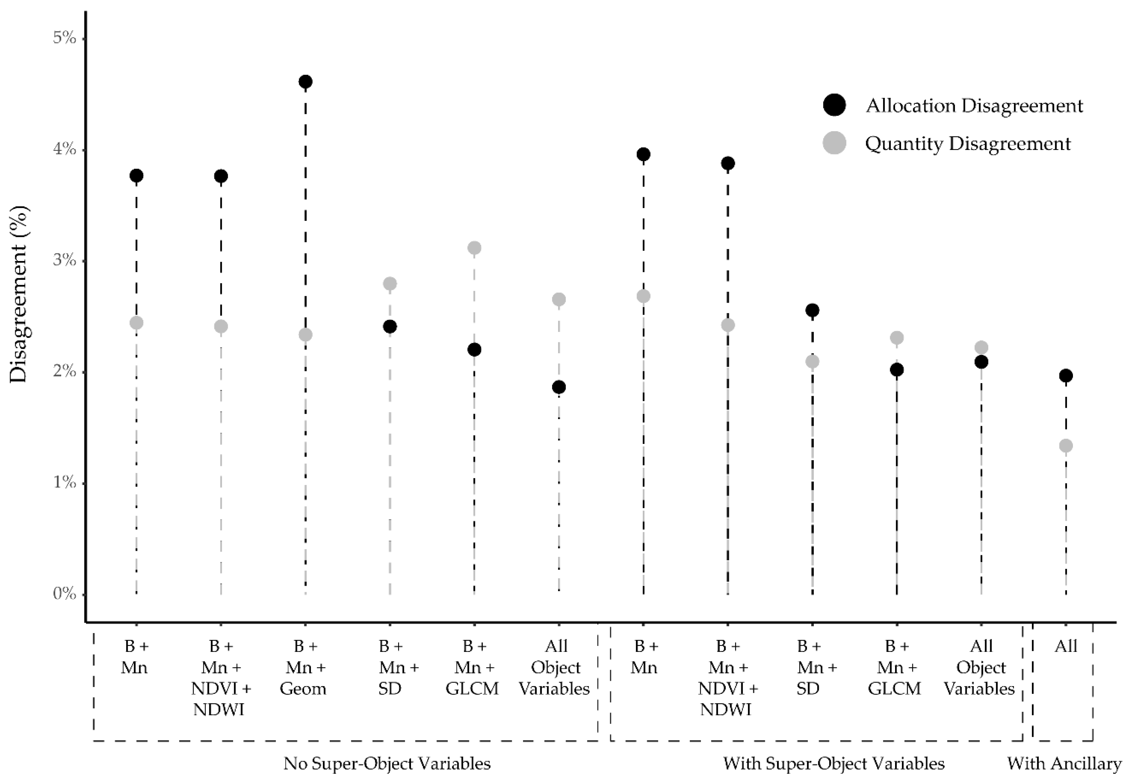
3.4. Feature Selection

Figure 5 shows the impact of variable selection as measured using overall accuracy, the Kappa statistic, quantity disagreement, allocation disagreement, and class user’s and producer’s accuracy. The results generally suggest that RF is robust to a large feature space, as performance tended to not change or decreased as the number of features was reduced. For example, the overall accuracy and Kappa statistics were 96.5% and 0.879, respectively, when using the top 25% of the variables in comparison to 96.7% and 0.886 when using all variables. Although this difference was statistically significant (z-score = 6.353), adding the additional variable only increased the accuracy by 0.2%. This study supports prior research that suggests that RF is robust to a complex and high dimensional feature space [15,55,56,57]. This research suggests that RF would be a good algorithm choice if many features will be used and no feature selection will be applied.

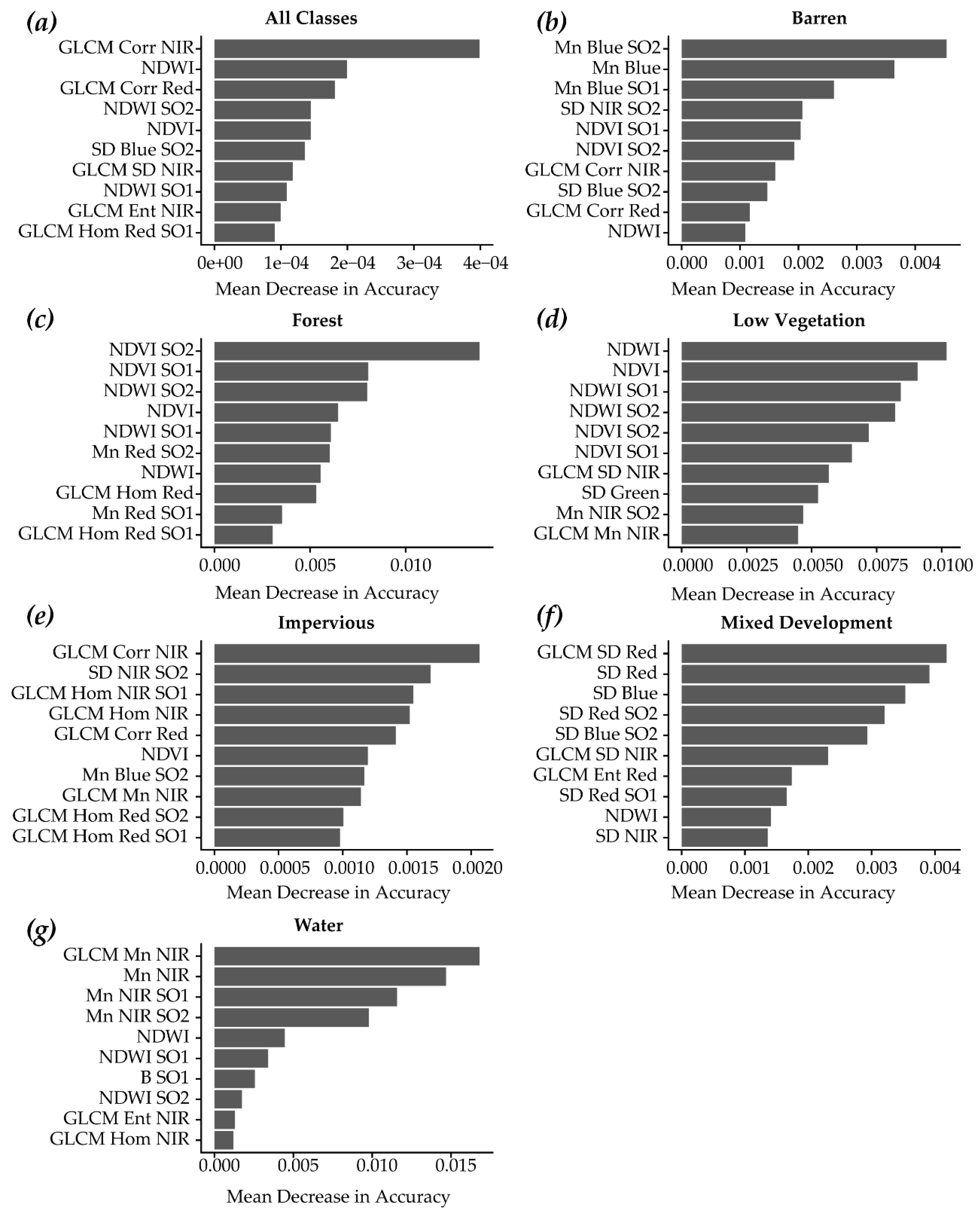
3.5. Variable Importance

Figure 6 provides the conditional variable importance of the top ten variables for the entire model (Figure 6a) and for each individual class (Figure 6b–g) using all input features. For mapping all six classes, many ancillary measures were found to be important, including mean structure density (Str), topographic slope (slp), Census block density (Blk), and road density (Rd), highlighting the value of incorporating ancillary variables. Further, mean structure density and mean topographic slope were found to be the most important variables. Important spectral variables include NDVI and Mean NIR (Mn NIR). Additionally, measures calculated at super-object levels were found to be important, including NDVI and NDWI, suggesting that incorporating super-object measures was of value. It is interesting that NDVI and NDWI were found to be important variables; however, as discussed above, the incorporation of these variables did not statistically significantly improve the classification accuracy. A possible reason for this is that the algorithm may be able to obtain the comparable information from the bands used to calculate the indices.

Many variables were found to be of particular importance for specific classes. For example, topographic slope (Slp) and mean road density (Rd) were valuable for mapping impervious surfaces. Generally, classes that were more spectrally distinct did not show high importance for the ancillary data; for example, the only ancillary variable in the top ten for the water class was mean topographic slope, and no ancillary variable were in the top ten for forest. This highlights the value of including ancillary variable when classes that may be spectrally confused, such as impervious surfaces and barren areas, are to be mapped.

Figure 7 shows conditional variable importance when the ancillary variables were excluded. Once the ancillary measures were removed, textural measures became more important in the model. For example, NIR GLCM correlation (GLCM Corr NIR) was found to be the most important variable. This suggests that textural measures may be of value if ancillary data are not available and classes that are spectrally confused are to be separated. GLCM correlation, entropy, homogeneity, and standard deviation were all found to be of value. Measures from super-objects were also found to be important, including band indices, band means, and textural measures. No measures of object geometry were included in the top list of variables for any class, supporting our previous finding that geometric measures did not improve classification accuracy.

4. Discussion

Land cover classification was performed for the entire state of West Virginia using a combination of GEOBIA, RF machine learning, and publicly available orthophotography and ancillary data. The best classification accuracy obtained was 96.7% (Kappa = 0.886) using a balanced training dataset and all variables. Forest, low vegetation, and water were mapped with user’s and producer’s accuracies above 85%. In contrast, the barren, impervious, and mixed developed classes were more difficult to map. In this section, we will make some recommendations regarding general land cover classification over large spatial extents as highlighted by our findings and in the context of previous studies.

4.1. Sample Size and Feature Selection

The number and quality of training samples have been shown to have a large impact on classification accuracy [3,28]; however, RF has been found to be more robust to both reduced training data size and quality in comparison to other algorithms [3,29]. In this study, we found that classification accuracy stabilized fairly rapidly. If abundant training data are an issue in a mapping project, we suggest experimenting with the available data to determine if an adequate output is obtained. If adequate results are not obtained, then additional data may need to be collected. Although data and landscape heterogeneity can complicate mapping tasks over large spatial extent [1,2,3,4,5,6], large areas offer the benefit that large training datasets can be produced. Although time-consuming to collect, these data could be reused in later mapping projects. For example, available training datasets could be assessed for change and used to classify different imagery to assess landscape change or update the land cover product on a regular basis. As quality training data are important, we recommend investing resources to create a quality training set, as this is one of the most important factors in obtaining an accurate classification.

This study supports previous research that suggests that the RF algorithm is robust to complex and high dimensional feature spaces [3,26,29]. Feature selection did not improve the classification performance, and accuracy tended to decrease with substantial variable reduction. Overall accuracy only dropped by 0.2% when 25% of the variables were used, so, even if feature selection does not improve the classification accuracy, it may still be worth pursuing as a means to simplify the model. This may be especially appealing for large-area mapping projects so that a large number of variables do not need to be generated across a large spatial extent for a large number of image objects. If variable selection will be undertaken, we suggest assessing important features over smaller study areas so that only the important features will need to be generated for the entire mapping extent.

4.2. Value of Super-Object Variables

We obtained mixed results when incorporating super-object attributes, in contrast to Johnson [51] and Johnson et al. [52]. Although incorporating these measures only increased accuracy slightly, some super-group measures were found to be of high importance in the classification based on RF-derived conditional variable importance. There is a large computational demand when multiple segmentations must be performed for a large mapping extent, so it is questionable whether this added complexity and processing time justifies only a slight increase in accuracy. However, super-objects may be considered as a means to potentially improve classification accuracy if the image used offers few bands or no ancillary data are available.

4.3. Value of Measures of Texture and Object Geometry

This study suggests the value of including a wide variety of variables. Both first-order texture, as standard deviation, and second-order texture, in terms of GLCM measures, were found to improve classification accuracy in this study whereas object geometry and band indices did not provide an improvement. Textural measures may be particularly appealing when no ancillary data are available, such as LiDAR, as suggested by O’Neil-Dunne et. al. [4]. As noted by Warner [46], the value of textural measures may be case-specific; however, we suggest that they be explored as an option if classification accuracy does not prove to be adequate using only the central tendency measures or when ancillary data are limited. Image object geometric measures were found to be of little value in this classification task.

4.4. Value of Ancillary Data

Many studies have found improved classification accuracy when ancillary data are included [2,3,4,19,21,39,47,49,57], which this research also supports. Further, this appears to be especially true if spectrally similar classes are to be mapped. Although the ancillary data used here were limited, we still observed a 1.0% increase in the classification accuracy in comparison to using only the image-derived variables and object geometric measures. Unfortunately, quality ancillary data, such as LiDAR or parcel boundaries, may be incomplete or inconsistent over large mapping extents or expensive to acquire. We suggest an inventory of available data be completed prior to undertaking a classification task. One of the benefits of using GEOBIA is the ability to summarize a variety of disparate datasets relative to image objects [39].

4.5. Practical Recommendations for Mapping Large Areas

Many challenges arose while attempting to complete this mapping project over a large spatial extent. First, due to spectral and landscape heterogeneity, we found it necessary to collect a large number of training and validation samples, which required several hundred analyst hours. It was not possible to mosaic the entire NAIP image dataset; instead segmentation, attribute calculation, and classification had to be performed separately for each of the 1830 tiles. We found that providing a 600 m overlap between adjacent tiles helped reduce any edge effects, as no edges or tile boundaries are observable in the final dataset.

This process was simplified greatly using scripts and loops to perform the feature summarization in ArcGIS Pro and the classification in R. Access to eCognition Server was necessary to apply the segmentation and variable calculation processes to all image tiles. We were able to run this on a personal computer in under a week. However, access to parallel computing architecture would be necessary if this type of mapping was to be undertaken across a larger geospatial extent, such as the entirety of CONUS. Making use of Google Earth Engine or other cloud computing platforms may prove to be necessary to scale such an analysis.

5. Conclusions

Land cover mapping at a high spatial resolution and over large spatial extents can be challenging for a variety of reasons including large data volumes, computational load, processing time, complexity of developing training and validation datasets, data availability, and heterogeneity in data and landscape conditions. Fortunately, modern machine learning algorithms, such as RF, are generally robust to this complexity. In this study, we were able to obtain an overall accuracy of 96.7% and a Kappa statistic of 0.886 using a combination of GEOBIA, RF machine learning, and public imagery and ancillary data. The forest, low vegetation, and water classes were mapped with accuracy whereas the barren, impervious, and mixed developed classes proved more difficult to map, as suggested by the lower user’s and producer’s accuracies for these classes. There is complexity in defining and mapping classes that are impacted by land use, such as agriculture, as opposed to broader and more spectrally distinct land cover categories. Further, this highlights the need to investigate class-level accuracy as opposed to only overall accuracy.

This research suggests many additional questions that should be explored in order to further the use of high spatial resolution data to map large extents. There is a need to explore the impact of using training data and models produced in one location to map other areas, as training data creation is a time-consuming process. West Virginia is a landscape dominated by forest. There is a need to explore the mapping of other environments from data such as NAIP, such as arid environments and agricultural areas, and compare and assess challenges inherent to mapping land cover in different landscapes. Additionally, there is a need to further explore computational processes for processing large volumes of geospatial data efficiently. Specifically, future work should explore methods that rely solely on open-source software, such as R, QGIS, Orfeo Toolbox, and Python scripting, for large-area mapping to expand upon this work. Open-source technologies should specifically be explored in the context of cloud-based processing and parallel computing.

One complexity in this study was the variability in the input NAIP orthophotography over this large spatial extent. Although all images were leaf-on and represented similar phenological conditions, there were inconsistencies resulting from collection date and illuminating conditions. This is a major challenge in working with high spatial resolution aerial imagery over large spatial extents, and there is still a need to investigate means to combat this issue.

Accuracy assessment over this large spatial extent was also a challenge. Appropriate accuracy assessment methods for GEOBIA classifications are still being actively debated. There is a need for additional research to define standard GEOBIA accuracy assessment methods and offer guidance for more applied studies, and these methods should be robust to large study area extents and classifications schemes in which some classes make up a small proportion of the landscape.

Given the importance of land cover data for a variety of mapping, assessment, and modeling tasks, it is important to continue to pursue advanced methods—such as deep learning—for extracting information from high resolution imagery. Specifically, there should be a focus on processes that are robust and scalable to large spatial extents.

References

1. Basu, S.; Ganguly, S.; Nemani, R.R.; Mukhopadhyay, S.; Zhang, G.; Milesi, C.; Michaelis, A.; Votava, P.; Dubayah, R.; Duncanson, L.; et al. A semiautomated probabilistic framework for tree-cover delineation from 1-m NAIP imagery using a high-performance computing architecture. IEEE Trans. Geosci. Remote Sens. 2015, 53, 5690–5708. [Google Scholar] [CrossRef]
2. Li, X.; Shao, G. Object-based land-cover mapping with high resolution aerial photography at a county scale in midwestern USA. Remote Sens. 2014, 6, 11372–11390. [Google Scholar] [CrossRef]
3. Maxwell, A.E.; Warner, T.A.; Fang, F. Implementation of machine-learning classification in remote sensing: An applied review. Int. J. Remote Sens. 2018, 39, 2784–2817. [Google Scholar] [CrossRef]
4. O’Neil-Dunne, J.; MacFaden, S.; Royar, A. A versatile, production-oriented approach to high-resolution tree-canopy mapping in urban and suburban landscapes using GEOBIA and data fusion. Remote Sens. 2014, 6, 12837–12865. [Google Scholar] [CrossRef]
5. Pelletier, C.; Valero, S.; Inglada, J.; Champion, N.; Dedieu, G. Assessing the robustness of Random Forests to map land cover with high resolution satellite image time series over large areas. Remote Sens. Env. 2016, 187, 156–168. [Google Scholar] [CrossRef]
6. Ramezan, C.A.; Warner, T.A.; Maxwell, A.E. Evaluation of sampling and cross-validation tuning strategies for regional-scale machine learning classification. Remote Sens. 2019, 11, 185. [Google Scholar] [CrossRef]
7. Yang, L.; Jin, S.; Danielson, P.; Homer, C.; Gass, L.; Bender, S.M.; Case, A.; Costello, C.; Dewitz, J.; Fry, J.; et al. A new generation of the United States National Land Cover Database: Requirements, research priorities, design, and implementation strategies. ISPRS J. Photogramm. Remote Sens. 2018, 146, 108–123. [Google Scholar] [CrossRef]
8. Feranec, J.; Jaffrain, G.; Soukup, T.; Hazeu, G. Determining changes and flows in European landscapes 1990–2000 using CORINE land cover data. Appl. Geogr. 2010, 30, 19–35. [Google Scholar] [CrossRef]
9. Vitousek, P.M. Beyond Global Warming: Ecology and Global Change. Ecology 1994, 75, 1861–1876. [Google Scholar] [CrossRef]
10. Haines-Young, R. Land use and biodiversity relationships. Land Use Futur. 2009, 26, S178–S186. [Google Scholar] [CrossRef]
11. Hansen, M.C.; Loveland, T.R. A review of large area monitoring of land cover change using Landsat data. Landsat Leg. Spec. Issue 2012, 122, 66–74. [Google Scholar] [CrossRef]
12. Feddema, J.J. The importance of land-cover change in simulating future climates. Science 2005, 310, 1674–1678. [Google Scholar] [CrossRef] [PubMed]
13. Land Cover Data Project. Available online: https://chesapeakeconservancy.org/conservation-innovation-center/high-resolution-data/land-cover-data-project-2/ (accessed on 12 March 2019).
14. Pixel-Level Land Cover Classification Using the Geo AI Data Science Virtual Machine and Batch AI. Available online: https://blogs.technet.microsoft.com/machinelearning/2018/03/12/pixel-level-land-cover-classification-using-the-geo-ai-data-science-virtual-machine-and-batch-ai/ (accessed on 12 March 2019).
15. Breiman, L. Random forests. Mach. Learn. 2001, 45, 5–32. [Google Scholar] [CrossRef]
16. Gislason, P.O.; Benediktsson, J.A.; Sveinsson, J.R. Random Forests for land cover classification. Pattern Recognit. Remote Sens. PRRS 2004 2006, 27, 294–300. [Google Scholar] [CrossRef]
17. Pal, M. Random Forest classifier for remote sensing classification. Int. J. Remote Sens. 2005, 26, 217–222. [Google Scholar] [CrossRef]
18. Pal, M.; Mather, P.M. Decision tree based classification of remotely sensed data. In Proceedings of the 22nd Asian Conference on Remote Sensing, Singapore, 5–9 November 2001; p. 9. [Google Scholar]
19. Guo, L.; Chehata, N.; Mallet, C.; Boukir, S. Relevance of airborne lidar and multispectral image data for urban scene classification using Random Forests. ISPRS J. Photogramm. Remote Sens. 2011, 66, 56–66. [Google Scholar] [CrossRef]
20. Ruiz Hernandez, I.E.; Shi, W. A Random Forests classification method for urban land-use mapping integrating spatial metrics and texture analysis. Int. J. Remote Sens. 2018, 39, 1175–1198. [Google Scholar] [CrossRef]
21. Maxwell, A.E.; Warner, T.A.; Strager, M.P.; Pal, M. Combining RapidEye satellite imagery and Lidar for mapping of mining and mine reclamation. Photogramm. Eng. Remote Sens. 2014, 80, 179–189. [Google Scholar] [CrossRef]
22. Hayes, M.M.; Miller, S.N.; Murphy, M.A. High-resolution landcover classification using Random Forest. Remote Sens. Lett. 2014, 5, 112–121. [Google Scholar] [CrossRef]
23. Lawrence, R.L.; Moran, C.J. The AmericaView classification methods accuracy comparison project: A rigorous approach for model selection. Remote Sens. Env. 2015, 170, 115–120. [Google Scholar] [CrossRef]
24. Ma, L.; Li, M.; Ma, X.; Cheng, L.; Du, P.; Liu, Y. A review of supervised object-based land-cover image classification. ISPRS J. Photogramm. Remote Sens. 2017, 130, 277–293. [Google Scholar] [CrossRef]
25. Khoshgoftaar, T.M.; Golawala, M.; Hulse, J.V. An empirical study of learning from imbalanced data using random forest. In Proceedings of the 19th IEEE International Conference on Tools with Artificial Intelligence (ICTAI 2007), Patras, Greece, 29–31 October 2007; IEEE: Piscataway, NJ, USA; pp. 310–317. [Google Scholar]
26. Rodriguez-Galiano, V.F.; Ghimire, B.; Rogan, J.; Chica-Olmo, M.; Rigol-Sanchez, J.P. An assessment of the effectiveness of a random forest classifier for land-cover classification. ISPRS J. Photogramm. Remote Sens. 2012, 67, 93–104. [Google Scholar] [CrossRef]
27. Shi, D.; Yang, X. An assessment of algorithmic parameters affecting image classification accuracy by Random Forests. Photogramm. Eng. Remote Sens. 2016, 82, 407–417. [Google Scholar]
28. Huang, C.; Davis, L.S.; Townshend, J.R.G. An assessment of support vector machines for land cover classification. Int. J. Remote Sens. 2002, 23, 725–749. [Google Scholar] [CrossRef]
29. Ghimire, B.; Rogan, J.; Galiano, V.R.; Panday, P.; Neeti, N. An evaluation of bagging, boosting, and Random Forests for land-cover classification in Cape Cod, Massachusetts, USA. GIScience Remote Sens. 2012, 49, 623–643. [Google Scholar] [CrossRef]
30. Blagus, R.; Lusa, L. Class prediction for high-dimensional class-imbalanced data. BMC Bioinform. 2010, 11. [Google Scholar] [CrossRef] [PubMed]
31. Haibo, H.; Garcia, E.A. Learning from imbalanced data. IEEE Trans. Knowl. Data Eng. 2009, 21, 1263–1284. [Google Scholar] [CrossRef]
32. Stumpf, A.; Kerle, N. Object-oriented mapping of landslides using Random Forests. Remote Sens. Env. 2011, 115, 2564–2577. [Google Scholar] [CrossRef]
33. Waske, B.; Benediktsson, J.A.; Sveinsson, J.R. Classifying remote sensing data with support vector machines and imbalanced training data. In Multiple Classifier Systems, Proceedings of the 8th International Workshop, MCS 2009, Reykjavik, Iceland, 10–12 June 2009; Benediktsson, J.A., Kittler, J., Roli, F., Eds.; Springer: Berlin/Heidelberg, Germany; pp. 375–384.
34. Baker, B.A.; Warner, T.A.; Conley, J.F.; McNeil, B.E. Does spatial resolution matter? A multi-scale comparison of object-based and pixel-based methods for detecting change associated with gas well drilling operations. Int. J. Remote Sens. 2013, 34, 1633–1651. [Google Scholar] [CrossRef]
35. Blaschke, T. Object based image analysis for remote sensing. ISPRS J. Photogramm. Remote Sens. 2010, 65, 2–16. [Google Scholar] [CrossRef] [Green Version]
36. Blaschke, T.; Hay, G.J.; Kelly, M.; Lang, S.; Hofmann, P.; Addink, E.; Queiroz Feitosa, R.; van der Meer, F.; van der Werff, H.; van Coillie, F.; et al. Geographic object-based image analysis—Towards a new paradigm. ISPRS J. Photogramm. Remote Sens. 2014, 87, 180–191. [Google Scholar] [CrossRef] [PubMed]
37. Chubey, M.S.; Franklin, S.E.; Wulder, M.A. Object-based analysis of Ikonos-2 imagery for extraction of forest inventory parameters. Photogramm. Eng. Remote Sens. 2006, 72, 383–394. [Google Scholar] [CrossRef]
38. Drăguţ, L.; Blaschke, T. Automated classification of landform elements using object-based image analysis. Geomorphology 2006, 81, 330–344. [Google Scholar] [CrossRef]
39. Maxwell, A.E.; Warner, T.A.; Strager, M.P.; Conley, J.F.; Sharp, A.L. Assessing machine-learning algorithms and image- and lidar-derived variables for GEOBIA classification of mining and mine reclamation. Int. J. Remote Sens. 2015, 36, 954–978. [Google Scholar] [CrossRef]
40. Meneguzzo, D.M.; Liknes, G.C.; Nelson, M.D. Mapping trees outside forests using high-resolution aerial imagery: A comparison of pixel- and object-based classification approaches. Env. Monit. Assess. 2013, 185, 6261–6275. [Google Scholar] [CrossRef] [PubMed]
41. Walter, V. Object-based classification of remote sensing data for change detection. ISPRS J. Photogramm. Remote Sens. 2004, 58, 225–238. [Google Scholar] [CrossRef]
42. Guo, Q.; Kelly, M.; Gong, P.; Liu, D. An object-based classification approach in mapping tree mortality using high spatial resolution imagery. GIScience Remote Sens. 2007, 44, 24–47. [Google Scholar] [CrossRef]
43. Kim, M.; Madden, M.; Warner, T.A. Forest type mapping using object-specific texture measures from multispectral ikonos imagery. Photogramm. Eng. Remote Sens. 2009, 75, 819–829. [Google Scholar] [CrossRef]
44. Haralick, R.M.; Shanmugam, K.S. Combined spectral and spatial processing of ERTS imagery data. Remote Sens. Env. 1974, 3, 3–13. [Google Scholar] [CrossRef] [Green Version]
45. Hall-Beyer, M. Practical guidelines for choosing GLCM textures to use in landscape classification tasks over a range of moderate spatial scales. Int. J. Remote Sens. 2017, 38, 1312–1338. [Google Scholar] [CrossRef]
46. Warner, T. Kernel-based texture in remote sensing image classification. Geogr. Compass 2011, 5, 781–798. [Google Scholar] [CrossRef]
47. Maxwell, A.E.; Warner, T.A. Differentiating mine-reclaimed grasslands from spectrally similar land cover using terrain variables and object-based machine learning classification. Int. J. Remote Sens. 2015, 36, 4384–4410. [Google Scholar] [CrossRef] [Green Version]
48. Bishop, B.; Dietterick, B.; White, R.; Mastin, T. Classification of plot-level fire-caused tree mortality in a redwood forest using digital orthophotography and LiDAR. Remote Sens. 2014, 6, 1954–1972. [Google Scholar] [CrossRef]
49. Guan, H.; Li, J.; Chapman, M.; Deng, F.; Ji, Z.; Yang, X. Integration of orthoimagery and lidar data for object-based urban thematic mapping using Random Forests. Int. J. Remote Sens. 2013, 34, 5166–5186. [Google Scholar] [CrossRef]
50. Zhou, W.; Troy, A.; Grove, M. Object-based land cover classification and change analysis in the Baltimore metropolitan area using multitemporal high resolution remote sensing data. Sensors 2008, 8, 1613–1636. [Google Scholar] [CrossRef] [PubMed]
51. Johnson, B.A. High-resolution urban land-cover classification using a competitive multi-scale object-based approach. Remote Sens. Lett. 2013, 4, 131–140. [Google Scholar] [CrossRef]
52. Johnson, B.; Xie, Z. Classifying a high resolution image of an urban area using super-object information. ISPRS J. Photogramm. Remote Sens. 2013, 83, 40–49. [Google Scholar] [CrossRef]
53. Hughes, G. On the mean accuracy of statistical pattern recognizers. IEEE Trans. Inf. Theory 2006, 14, 55–63. [Google Scholar] [CrossRef]
54. Pal, M.; Mather, P.M. An assessment of the effectiveness of decision tree methods for land cover classification. Remote Sens. Env. 2003, 86, 554–565. [Google Scholar] [CrossRef]
55. Chan, J.C.-W.; Paelinckx, D. Evaluation of Random Forest and Adaboost tree-based ensemble classification and spectral band selection for ecotope mapping using airborne hyperspectral imagery. Remote Sens. Env. 2008, 112, 2999–3011. [Google Scholar] [CrossRef]
56. Lawrence, R.L.; Wood, S.D.; Sheley, R.L. Mapping invasive plants using hyperspectral imagery and Breiman Cutler classifications (randomForest). Remote Sens. Env. 2006, 100, 356–362. [Google Scholar] [CrossRef]
57. Duro, D.C.; Franklin, S.E.; Dubé, M.G. Multi-scale object-based image analysis and feature selection of multi-sensor earth observation imagery using random forests. Int. J. Remote Sens. 2012, 33, 4502–4526. [Google Scholar] [CrossRef]
58. Genuer, R.; Poggi, J.-M.; Tuleau-Malot, C. Variable selection using Random Forests. Pattern Recognit. Lett. 2010, 31, 2225–2236. [Google Scholar] [CrossRef]
59. Strobl, C.; Boulesteix, A.-L.; Kneib, T.; Augustin, T.; Zeileis, A. Conditional variable importance for random forests. BMC Bioinform. 2008, 9, 307. [Google Scholar] [CrossRef] [PubMed]
60. Maxwell, A.E.; Warner, T.A.; Vanderbilt, B.C.; Ramezan, C.A. Land cover classification and feature extraction from national agriculture imagery program (NAIP) Orthoimagery: A Review. Photogramm. Eng. Remote Sens. 2017, 83, 737–747. [Google Scholar] [CrossRef]
61. Zhou, Y.; Wang, Y.Q. An Assessment of impervious surface areas in Rhode Island. Northeast. Nat. 2007, 14, 643–650. [Google Scholar] [CrossRef]
62. Maxwell, A.E.; Strager, M.P.; Warner, T.A.; Zégre, N.P.; Yuill, C.B. Comparison of NAIP orthophotography and RapidEye satellite imagery for mapping of mining and mine reclamation. GIScience Remote Sens. 2014, 51, 301–320. [Google Scholar] [CrossRef]
63. Gong, P.; Howarth, P.J. Land-use classification of SPOT HRV data using a cover-frequency method. Int. J. Remote Sens. 1992, 13, 1459–1471. [Google Scholar] [CrossRef]
64. Strahler, A.H.; Woodcock, C.E.; Smith, J.A. On the nature of models in remote sensing. Remote Sens. Env. 1986, 20, 121–139. [Google Scholar] [CrossRef]
65. Yu, Q.; Gong, P.; Clinton, N.; Biging, G.; Kelly, M.; Schirokauer, D. Object-based Detailed Vegetation Classification with Airborne High Spatial Resolution Remote Sensing Imagery. Available online: https://www.ingentaconnect.com/content/asprs/pers/2006/00000072/00000007/art00004# (accessed on 14 March 2019).
66. Davies, K.W.; Petersen, S.L.; Johnson, D.D.; Bracken Davis, D.; Madsen, M.D.; Zvirzdin, D.L.; Bates, J.D. Estimating juniper cover from National Agriculture Imagery Program (NAIP) imagery and evaluating relationships between potential cover and environmental variables. Rangel. Ecol. Manag. 2010, 63, 630–637. [Google Scholar] [CrossRef]
67. Gartner, M.H.; Veblen, T.T.; Leyk, S.; Wessman, C.A. Detection of mountain pine beetle-killed ponderosa pine in a heterogeneous landscape using high-resolution aerial imagery. Int. J. Remote Sens. 2015, 36, 5353–5372. [Google Scholar] [CrossRef]
68. Yuan, F. Land-cover change and environmental impact analysis in the Greater Mankato area of Minnesota using remote sensing and GIS modelling. Int. J. Remote Sens. 2008, 29, 1169–1184. [Google Scholar] [CrossRef]
69. Crimmins, S.M.; Mynsberge, A.R.; Warner, T.A. Estimating woody browse abundance from aerial imagery. Int. J. Remote Sens. 2009, 30, 3283–3289. [Google Scholar] [CrossRef]
70. Nagel, P.; Yuan, F. High-resolution land cover and impervious surface classifications in the twin cities metropolitan area with NAIP imagery. Photogramm. Eng. Remote Sens. 2016, 82, 63–71. [Google Scholar] [CrossRef]
71. Pierce, K. Accuracy Optimization for high resolution object-based change detection: An example mapping regional urbanization with 1-m aerial imagery. Remote Sens. 2015, 7, 12654–12679. [Google Scholar] [CrossRef]
72. Strausbaugh, P.D. Flora of West Virginia; Seneca Books: Grantsville, WV, USA, 1978; ISBN 978-0-89092-010-7. [Google Scholar]
73. Erdas Imagine 2018; Hexagon Geospatial: Madison, AL, USA, 2018.
74. ArcGIS Pro 2.2; ESRI: Redlands, CA, USA, 2018.
75. Computer Generated Building Footprints for the United States: Microsoft/USBuildingFootprints; Microsoft: Redmond, WA, USA, 2019.
76. eCognition Developer 9; Trimble: Sunnyvale, CA, USA, 2019.
77. Baatz, M.; Schäpe, A. Multiresolution segmentation: An optimization approach for high quality multi-scale image segmentation. ISPRS Int. Arch. Photogramm. Remote Sens. Spat. Inf. Sci. 2000, 12–23. [Google Scholar]
78. Liu, D.; Xia, F. Assessing object-based classification: Advantages and limitations. Remote Sens. Lett. 2010, 1, 187–194. [Google Scholar] [CrossRef]
79. Myint, S.W.; Gober, P.; Brazel, A.; Grossman-Clarke, S.; Weng, Q. Per-pixel vs. object-based classification of urban land cover extraction using high spatial resolution imagery. Remote Sens. Env. 2011, 115, 1145–1161. [Google Scholar] [CrossRef]
80. Drăguţ, L.; Csillik, O.; Eisank, C.; Tiede, D. Automated parameterisation for multi-scale image segmentation on multiple layers. ISPRS J. Photogramm. Remote Sens. 2014, 88, 119–127. [Google Scholar] [CrossRef]
81. Haralick, R.M.; Shanmugam, K.S.; Dinstein, I. Textural features for image classification. IEEE Trans Syst. Man Cybern. 1973, 3, 610–621. [Google Scholar] [CrossRef]
82. McFEETERS, S.K. The use of the Normalized Difference Water Index (NDWI) in the delineation of open water features. Int. J. Remote Sens. 1996, 17, 1425–1432. [Google Scholar] [CrossRef]
83. Foody, G.M. Thematic map comparison: Evaluating the statistical significance of differences in classification accuracy. Photogramm. Eng. Remote Sens. 2004, 70, 627–633. [Google Scholar] [CrossRef]
84. Foody, G.M. Status of land cover classification accuracy assessment. Remote Sens. Env. 2002, 80, 185–201. [Google Scholar] [CrossRef]
85. Stehman, S.V. Statistical rigor and practical utility in thematic map accuracy assessment. Photogramm. Eng. Remote Sens. 2001, 67, 727–734. [Google Scholar]
86. Stehman, S.V.; Czaplewski, R.L. Design and analysis for thematic map accuracy assessment: Fundamental principles. Remote Sens. Environ. 1998, 64, 331–344. [Google Scholar] [CrossRef]
87. Stehman, S.V. Selecting and interpreting measures of thematic classification accuracy. Remote Sens. Env. 1997, 62, 77–89. [Google Scholar] [CrossRef]
88. Stehman, S.V. Basic probability sampling designs for thematic map accuracy assessment. Int. J. Remote Sens. 1999, 20, 2423–2441. [Google Scholar] [CrossRef]
89. Stehman, S.V. A critical evaluation of the normalized error matrix in map accuracy assessment. Photogramm. Eng. Remote Sens. 2004, 70, 743–751. [Google Scholar] [CrossRef]
90. Stehman, S.V. Sampling designs for accuracy assessment of land cover. Int. J. Remote Sens. 2009, 30, 5243–5272. [Google Scholar] [CrossRef]
91. Stehman, S.V. Estimating area and map accuracy for stratified random sampling when the strata are different from the map classes. Int. J. Remote Sens. 2014, 35, 4923–4939. [Google Scholar] [CrossRef]
92. Liaw, A.; Wiener, M.C. Classification and regression by randomForest. R News 2007, 2/3, 18–22. [Google Scholar]
93. Kuhn, M.; Wing, J.; Weston, S.; Williams, A.; Keefer, C.; Engelhardt, A.; Cooper, T.; Mayer, Z.; Kenkel, B.; Benesty, M.; et al. Caret: Classification and Regression Training. R package version 6.0-73. Available online: https://cran.r-project.org/web/packages/caret/index.html (accessed on 12 March 2019).
94. R Core Team. R: A Language and Environment for Statistical Computing; R Foundation for Statistical Computing: Vienna, Austria, 2018. [Google Scholar]
95. Evans, J.S.; Cushman, S.A. Gradient modeling of conifer species using random forests. Landsc. Ecol. 2009, 24, 673–683. [Google Scholar] [CrossRef]
96. Strobl, C.; Boulesteix, A.-L.; Zeileis, A.; Hothorn, T. Bias in random forest variable importance measures: Illustrations, sources and a solution. BMC Bioinform. 2007, 8, 25. [Google Scholar] [CrossRef] [PubMed]
97. Maxwell, A.E.; Warner, T.A.; Strager, M.P. Predicting palustrine wetland probability using random forest machine learning and digital elevation data-derived terrain variables. Photogramm. Eng. Remote Sens. 2016, 82, 437–447. [Google Scholar] [CrossRef]
98. Pontius, R.G.; Millones, M. Death to Kappa: Birth of quantity disagreement and allocation disagreement for accuracy assessment. Int. J. Remote Sens. 2011, 32, 4407–4429. [Google Scholar] [CrossRef]
99. Pontius, R.G. Quantification error versus location error in comparison of categorical maps. Photogramm. Eng. Remote Sens. 2000, 66, 1011–1016. [Google Scholar]
100. Congalton, R.G.; Green, K. Assessing the Accuracy of Remotely Sensed Data: Principles and Practices; CRC Press: Boca Raton, FL, USA, 2008. [Google Scholar]
101. MacLean, M.G.; Congalton, D.R.G. Map accuracy assessment issues when using an object-oriented approach. In Proceedings of the American Society for Photogrammetry and Remote Sensing 2012 Annual Conference, Sacramento, CA, USA, 19–23 March 2012; p. 5. [Google Scholar]
102. Dietterich, T.G. Approximate statistical tests for comparing supervised classification learning algorithms. Neural Comput. 1998, 10, 1895–1923. [Google Scholar] [CrossRef] [PubMed]
103. Radoux, J.; Bogaert, P.; Fasbender, D.; Defourny, P. Thematic accuracy assessment of geographic object-based image classification. Int. J. Geogr. Inf. Sci. 2011, 25, 895–911. [Google Scholar] [CrossRef]
104. Radoux, J.; Bogaert, P. Accounting for the area of polygon sampling units for the prediction of primary accuracy assessment indices. Remote Sens. Env. 2014, 142, 9–19. [Google Scholar] [CrossRef]
105. Radoux, J.; Bogaert, P. Good practices for object-based accuracy assessment. Remote Sens. 2017, 9, 646. [Google Scholar] [CrossRef]
106. Stehman, S.V.; Wickham, J.D. Pixels, blocks of pixels, and polygons: Choosing a spatial unit for thematic accuracy assessment. Remote Sens. Env. 2011, 115, 3044–3055. [Google Scholar] [CrossRef]
107. Ye, S.; Pontius, R.G.; Rakshit, R. A review of accuracy assessment for object-based image analysis: From per-pixel to per-polygon approaches. ISPRS J. Photogramm. Remote Sens. 2018, 141, 137–147. [Google Scholar] [CrossRef]
Figure 1. Land cover classification result example. Regions were selected to highlight results for areas with different land cover conditions and so that the result could be viewed at different scales and spatial extents.
Remotesensing 11 01409 g001
Figure 2. Overall accuracy and Kappa comparison for different feature spaces.
Remotesensing 11 01409 g002
Figure 3. Quantity and allocation disagreement comparison for different feature spaces.
Remotesensing 11 01409 g003
Figure 4. These graphs show results when using all image-derived and ancillary variables. (a) Change in overall accuracy and Kappa with varying sample size. (b) Change in quantity and allocation disagreement with varying sample size. (c) Change in user’s accuracy per class with varying sample size. (d) Change in producer’s accuracy per class with varying sample size.
Remotesensing 11 01409 g004
Figure 5. These graphs show results when using all image-derived and ancillary variables. (a) Overall accuracy and Kappa vs percent of variables. (b) Quantity and allocation disagreement vs percent of variables. (c) User’s accuracy per class vs percent of variables (d) Producer’s accuracy per class vs percent of variables.
Remotesensing 11 01409 g005
Figure 6. Conditional variable importance when using all variables. (a) shows variable importance for the entire classification while (bg) show variable importance for a specific class. Acronyms are defined in Table 1.
Remotesensing 11 01409 g006
Figure 7. Conditional variable importance when using just the image-derived variables. (a) shows variable importance for the entire classification while (bg) show variable importance for a specific class. Acronyms are defined in Table 1.
Remotesensing 11 01409 g007