Article

Spatial Filtering in DCT Domain-Based Frameworks for Hyperspectral Imagery Classification

The State Key Laboratory of Information Engineering in Surveying, Mapping, and Remote Sensing, Wuhan University, Wuhan 430079, China
*
Author to whom correspondence should be addressed.
Remote Sens. 2019, 11(12), 1405; https://doi.org/10.3390/rs11121405
Submission received: 7 May 2019 / Revised: 10 June 2019 / Accepted: 11 June 2019 / Published: 13 June 2019
(This article belongs to the Special Issue Robust Multispectral/Hyperspectral Image Analysis and Classification)

Abstract

:
In this article, we propose two effective frameworks for hyperspectral imagery classification based on spatial filtering in Discrete Cosine Transform (DCT) domain. In the proposed approaches, spectral DCT is performed on the hyperspectral image to obtain a spectral profile representation, where the most significant information in the transform domain is concentrated in a few low-frequency components. The high-frequency components that generally represent noisy data are further processed using a spatial filter to extract the remaining useful information. For the spatial filtering step, both two-dimensional DCT (2D-DCT) and two-dimensional adaptive Wiener filter (2D-AWF) are explored. After performing the spatial filter, an inverse spectral DCT is applied on all transformed bands including the filtered bands to obtain the final preprocessed hyperspectral data, which is subsequently fed into a linear Support Vector Machine (SVM) classifier. Experimental results using three hyperspectral datasets show that the proposed framework Cascade Spectral DCT Spatial Wiener Filter (CDCT-WF_SVM) outperforms several state-of-the-art methods in terms of classification accuracy, the sensitivity regarding different sizes of the training samples, and computational time.

1. Introduction

Hyperspectral imagery is collected by hyperspectral remote sensors at hundreds of narrow spectral bands. It contains rich discriminative spectral and spatial characteristics regarding material surfaces [1]. This attribute makes hyperspectral imagery an interesting source of information for a wide variety of applications in areas such as agriculture, environmental planning, surveillance, target detection, medicine [2,3,4], etc. Most of these hyperspectral applications build upon classification tasks. The classification of hyperspectral images is often performed using supervised classification methods, in which the training of the classification model requires the availability of labeled samples.
However, supervised classification has issues related to the imbalance between the high dimensionality and the limited availability of the acquired training samples, leading to the Hughes phenomenon. Moreover, noises from the environment and optical sensors can further reduce the classification effectiveness. Thus, to address these problems, intensive work has been devoted to providing accurate classifiers for hyperspectral images including, SVM [5], random forests [6], neural networks [7,8], sparse representation [9,10], and active learning [11,12] methods. Notably, the SVM classifier is efficient [5], since it requires relatively few training samples to obtain high classification accuracy and robustness regarding the high spectral dimensionality [5]. Although these pixel-wise classifiers can fully use the spectral information in the hyperspectral imagery, the spatial dimension is not takenin consideration. Consequently, the resulting classification maps are corrupted with salt-and-pepper noise [13].
In recent years, the integration of spatial to spectral information in a classifier model has improved classification accuracy, eliminating salt-and-pepper noise in classification maps [14,15]. Subsequently, spectral-spatial classification methods have been proposed to improve the accuracy further. The proposed methods can be roughly divided into three basic paradigms in terms of the fusion stage of the spectral and the spatial information [16], including preprocessing-based classification [17,18], post-processing-based classification [19,20], and integrated classification [21,22]. If we use more than one basic paradigm, we obtain a hybrid classification [23,24]. For these different adopted paradigms, there are typical methodologies including structural filtering-based approaches [25,26], random field-based approaches [27,28], morphological profile (MP)-based approaches [29,30], deep learning-based approaches [31,32,33], sparse representation-based approaches (SRC) [34,35], and segmentation-based approaches such as hierarchical segmentation [36], graph cut [37], and superpixel [38] approaches.
The structural filtering methodology is one of the most studied methods for preprocessing hyperspectral imagery [16]. Compared with other spatial methodologies, spatial filtering is simple and easy to implement [39]. This advantage makes it very suitable for practical applications. Much research is currently underway using structural filtering to obtain contextual features. The simplest way is to extract the spatial information based on the moment criteria [40,41]. Performing local harmonic analysis is another research direction for the structural filtering. The related work includesspectral-spatial wavelet features proposed in [42], 3D wavelet feature extraction and classification [26], spectral-spatial Gabor features developed in [43,44]. Recently, the trend in structural filtering has shifted towards methods that extract features using adaptive structures [45], such as adaptive multidimensional wiener filtering [46]. Even though these methods perform effectively in some scenarios, they still do not make full use of spatial information and only exploit this information in the preprocessing feature extraction phase.
Based on the success of the structural filtering methodology for hyperspectral imagery classification, and aiming to exploit the spectral and spatial information fully, in this work, we propose two effectivespectral-spatial hyperspectral classification frameworks based on performing the spatial filtering process in the DCT transform domain. We perform a spectral DCT on the original dataset to separate the most significant information concentrated in a few low-frequency components from the noisy data embedded in the high-frequency components. Then, spatial filtering is performed on the separated noisy data in the frequency domain to extract the remaining meaningful information. In the spatial filtering step, both 2D-DCT and 2D-AWF are explored given their effectiveness in noise removal [47]. Indeed, the variation of the noise variance in the spectral dimension is, in general, more drastic than that in the spatial dimensions [48]. Thus, the proposed approach is based on exploring DCT energy compaction property in the spectral domain to preserve the valuable part of the spectral signature presented by few low-frequency coefficients where further spatial filtering is only performed on the high-frequency coefficients that represent details and noise. This methodology makes the filtering process very effective. Furthermore, as we fully exploit the spectral and spatial information, the SVM classifier is adopted in our framework for its robustness to the Hughes phenomenon, in addition to its good generalization capacity [5].
The main contributions of this paper are threefold. The first contribution is the application of the spatial filter in the transform domain on the noisy data rather than discarding this part of information as usually adopted by the feature extraction-based approaches [49,50]. Thus, the proposed framework makes full use of the filtered spectral and spatial information of the hyperspectral image. The second contribution concerns the simplicity of the tuning configuration. Indeed, recently the proposed classifiers have reached very high classification accuracy where the competitive difference between them is more related to their tuning configuration simplicity. Thus, we provide an effective framework for hyperspectral image classification that involves the tuning of only a couple of parameters regarding the spectral and the spatial filters respectively. The third contribution is the low computational time compared with the other spectral-spatial classification methods. Indeed, the efficient exploitation of the filtering process improves the classification performance in less computational time.
The rest of this paper is structured as follows. The mathematical formulation of DCT and Wiener filter are briefly introduced in Section 2. The proposed approaches are described in Section 3. Datasets and the evaluation process are presented in Section 4. Section 5 gives the experimental setup and reports the results with the related analysis. Finally, Section 6 outlines a summary and draws conclusions.

2. Materials and Methods

2.1. Discrete Cosine Transform (DCT)

The DCT termed the cosine basis function which represents a summation of cosine functions at different increasing frequencies [51]. Using these cosine basis functions, DCT compacts the energy of a signal in a few low-frequency DCT coefficients [50]. Thus, DCT is widely used in image and signal processing, particularly for data compression, due to its high “energy compaction” property [52,53].
From the viewpoint of signal processing, considering each pixel X as a discrete signal in N dimension space where x = [x0, x1, x2, …, xN−1], and N represents the number of the spectral bands. The DCT coefficients of this discrete signal X are defined as [52]:
{ d = [ d 0 ,   d 1 , , d N 1 ] T d 0 = 2 N n = 0 N 1 x n d u = 2 N n = 0 N 1 x n cos ( 2 n + 1 ) u π 2 N ; u = 1 , 2 , . N 1
where du represents the uth DCT coefficient in N dimension space and each vector d corresponds to the original pixel X. Our approach is based on transforming the original spectral feature space to a transform feature space by performing the spectral DCT (SDCT) on each pixel spectral curve.
The Inverse DCT is defined as:
X ( u ) = n = 0 N 1 c [ u ] d n cos ( u 2 π n N )
where X(u) is the uth IDCT reconstruction value, u = 0, 1, …, N − 1, dn is the nth DCT coefficient, c[u] = 1 for u = 0 and c[u] = 2 for u = 1, 2, …, N − 1.
The DCT algorithm is very effective owing to its symmetry and simplicity. It is a reliable replacement for a Fast Fourier Transform (FFT), as it considers the real components of the image data. Generally, FFT is used for general spectral analysis applications where DCT is frequently used in lossy data compression and denoising applications, given its ability to concentrate the energy of the signal in a small set of DCT coefficients. Moreover, using only “real-valued” cosine functions makes DCT computationally simpler than FFT, which is a complex algorithm using magnitude and phase [54].

2.2. 2D-Discrete Cosine Transform (2D-DCT)

The 2D-DCT is obtained by performing the DCT on the first dimension and then the second one. The 2D-DCT of an f [ m , n ] , which is N by N image pixels, is expressed by Equation (3):
F [ u , v ] = 1 N 2 m = 0 N 1 n = 0 N 1 f [ m , n ] cos [ ( 2 m + 1 ) u π / 2 N ] cos [ ( 2 n + 1 ) v π / 2 N ]
where F [ u , v ] is the (u,v)th 2D-DCT coefficient, f [ m , n ] is (m,n) value of the matrix f and (u,v) are the discrete frequency variables (0,0), …, (N − 1, N − 1).
The 2D basis functions are the multiplication result of the matrix row of 1D-basis functions with the same function matrix column. The basis function frequencies are increasing with regard to both the vertical and horizontal directions [51]. The 2D Inverse DCT is expressed by Equation (4):
f [ m , n ] = u = 0 N 1 v = 0 N 1 c [ u ] c [ v ] F [ u , v ] cos [ ( 2 u + 1 ) m π / 2 N ] cos [ ( 2 v + 1 ) n π / 2 N ]
where f [ m , n ] is the ( m , n )th IDCT reconstruction value, F[ u , v ] is the ( u , v )th 2D-DCT coefficients, c[λ] = 1 for λ = 0 and c[λ] = 2 for λ = 1, 2, …, N − 1.
Due to its energy concentration ability, DCT provides optimal decorrelation for images [55]. Thus, in our approach, after performing DCT to obtain a frequency profile where the meaningful information is compacted in few low-frequency components is retained, and further spatial filtering is executed on the high-frequency components by exploring the effectiveness of both 2D-DCT and 2D-AWF filtering in the transform domain.

2.3. Spatial Adaptive Wiener Filter (2D-AWF)

Hyperspectral imagery can be affected by two kinds of noise which are signal-independent noise and signal-dependent noise, many references [56,57] argue that only signal-independent noise needs be reduced, as it is the dominant component. This signal-independent noise is referred to as Additive White Gaussian Noise (AWGN) [58]. Therefore, in the spatial filtering step of our approach, we have also explored the most widely known spatial filter for AWGN removal, which is the 2D-AWF.
Indeed, the Wiener filter was proposed by Norbert Wiener during the 1940s; it is based on the minimization of the mean square error (MSE) between the output signal and the estimated signal [59]. The 2D-AWF filter applies the idea of the Wiener filter in the spatial domain. It estimates the image noise and filters the image based on this noise [60].
Considering an image x ( i , j ) corrupted with AWGN n ( i , j ) expressed as follows:
y ( i , j ) = x ( i , j ) + n ( i , j )
where x ( i , j ) is the original image and y ( i , j ) denotes the noisy image.
If we assume that the noise is stationary of zero mean, uncorrelated with the original image. The original image x ( i , j ) can be modeled by:
x ( i , j ) = m x + σ x w ( i , j )
where m x is the local mean and σ x is the standard deviation, and w ( i , j ) representsthe zero mean white noise of unit variance. The spatial Wiener filter that minimizes the (MSE) between the original image x ( i , j ) and the enhanced image x ^ ( i , j ) is expressed as follows [61]:
x ^ ( i , j ) = m x + σ x 2 σ x 2 + σ n 2 [ y ( i , j ) m x ]
In Equation (7), m x and σ x are estimated from the observed noisy image and updated for each pixel as proposed in the Lee filter [62]:
m ^ x ( i , j ) = 1 ( 2 m + 1 ) ( 2 n + 1 ) k = i m i + m l = j n j + n y ( k , l )
σ ^ y 2 ( i , j ) = 1 ( 2 m + 1 ) ( 2 n + 1 ) k = i m i + m l = j n j + n [ y ( k , l ) m ^ x ( i , j ) ] 2
In our approach, the filter size setting (2m + 1)(2n + 1)is fixed regarding the best-obtained classification accuracy.
σ ^ x 2 ( i , j ) = max { 0 , σ ^ y 2 ( i , j ) σ n 2 }
After substituting m ^ x ( i , j ) and σ ^ x ( i , j ) into Equation (7), it becomes
x ^ ( i , j ) =   m ^ x ( i , j ) + σ ^ x 2 ( i , j )   σ ^ x 2 ( i , j ) + σ n 2 [ y ( i , j ) m ^ x ( i , j ) ]
In our approach, 2D-AWF is explored as a spatial filter in the DCT domain to extract the useful information embedded in the high-frequency components resulting from the spectral filtering using SDCT.

3. The Proposed Approach

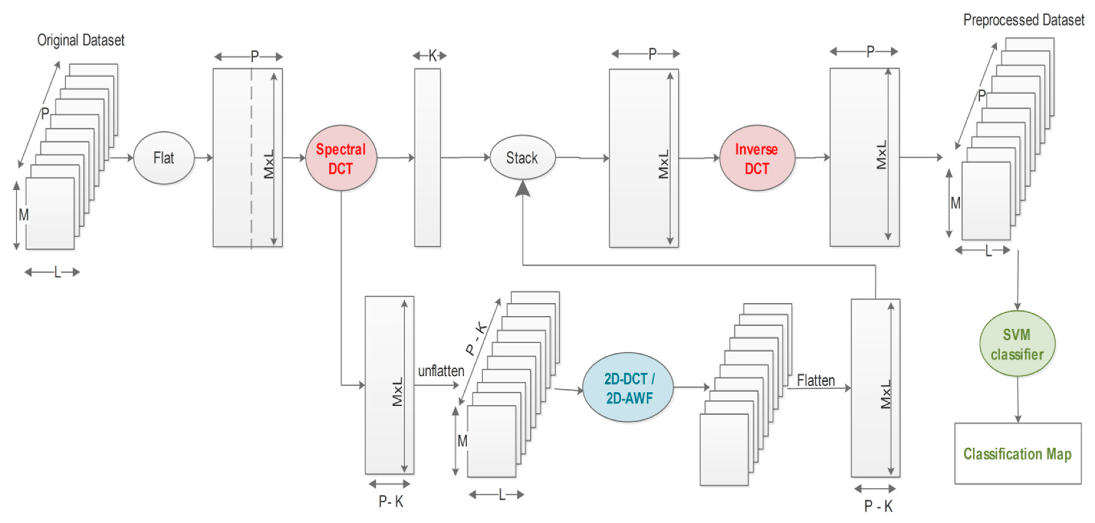
A general outline description of the proposed classification frameworks based on spectral DCT combined with a spatial filter (2D-DCT or 2D-AWF) and SVM classifier is provided in Figure 1.
As shown in Figure 1, in these approaches, we perform a spectral DCT on the original dataset to separate the most significant information concentrated in few low-frequency components from the noisy data embedded in the high-frequency components. Spatial filtering is performed in the transform domain on the high DCT spectral components to extract the remaining of meaningful information. An inverse spectral DCT is performed on all components including the filtered ones to obtain the final preprocessed hyperspectral dataset. Finally, the resulted data is introduced into the linear SVM classifier. Figure 2 provides a detailed flowchart of the proposed approaches.
As depicted in Figure 2, the proposed frameworks consist of the following steps:
Step 1: Consider an original hyperspectral dataset cube, with M rows, L columns, and P bands.
Step 2: Flatten the dataset cube to obtain a matrix E(N,P) with N = (M × L) rows and P columns.
Step 3: Perform a spectral DCT on matrix E to obtain two matrices: a matrix F(N,K) for the K first retained low-frequency components and matrix R(N,P-K) for the remaining high-frequency components (K is the cut-off channel count).
Step 4: Unflatten the matrix R(N,P-K) to obtain the data cube Rc(M,L,P-K) with M rows, L columns, and P-k bands.
Step 5: Perform spatial filtering on each matrix Rm(M, L) in the cube Rc using 2D-DCT or 2D-AWF as follows:
-
The 2D-DCT filtering step consists of performing a global 2D-DCT filter on each matrix Rm(M,L) where the high-frequency components are discarded using an empirical estimated hard threshold. Then, an inverse DCT is applied to the matrix Rm(M, L). Figure 3 illustrates this spatial filtering step.
-
2D-AWF approach filtering step consists on dividing the matrix Rm(M, L) into blocks or patches of a specified size and processing them using a local 2D-AWF.
Step 6: Flatten the filtered data cube Rc to get back to the matrix R.
Step 7: Stack the two matrices F and R in order to obtain the matrix D, which has the same size as the matrix E, in step 2.
Step 8: Perform an Inverse DCT on the matrix D to obtain the preprocessed matrix E.
Step 9: Unflatten matrix E to obtain the final matrix with same size as the original one (M × L × P) .

4. Data and Evaluation Process

4.1. Data

Three hyperspectral scenes with variant spatial resolutionsdownloaded from http://www.ehu.eus/ccwintco/index.php/Hyperspectral_Remote_Sensing_Scenes were used for the experiments including the Indian Pines, Salinas, and Pavia University datasets.
The first dataset concerns an Indian Pines scene. This scene was captured over northwest Indiana’s Indian Pines area by the Airborne Visible Infrared Imaging Spectrometer (AVIRIS) at a low spatial resolution of 20 m. This dataset has 220 bands of size 145 × 145 pixels where the bands affected by noise and water absorption were discarded leaving 200 bands. The ground reference data contains 16 classes. Regarding the spectral similarity between the classes and its low spatial resolution, this scene represents challenging classification. Table 1 lists the related classes and describes the number of samples, the training, and the test points in this dataset.
Figure 4 shows the original band and the ground truth data of the Indian Pines dataset.
The second test dataset was the Salinas scene. This dataset was captured the area over Salinas Valley in California by AVIRIS (Airborne Visible Infrared Imaging Spectrometer) at 3.7 m spatial resolution. This image comprises 220 bands of size 512 × 217 pixels where the bands affected by noise and water absorption were discarded, leaving 204 bands. There are 16 classes, representing a variety of crops in the ground reference data. Table 2 lists these classes with the related number of samples, training, and testing points in this dataset. Figure 5 illustrates the Salinas image and its ground truth categorization maps.
The third test dataset was the Pavia University scene. This scene was captured by the ROSIS sensor over the Pavia area, northern Italy. It has 610 × 610 pixels with 1.3 m spatial resolution and contains 103 spectral bands. For classification purposes, the scene is divided into nine regions as listed in Table 3 with the number of samples that belong to each region, the number of training and testing points.
Figure 6 illustrates the Pavia University image and its related ground truth maps.

4.2. Evaluation Process

Several state-of-the-art methods were considered for comparison to validate the effectiveness of our proposed CDCT-WF_SVM and CDCT-2DCT_SVM frameworks. These included two pixel-wise classifiers represented by the standard SVM [5], and PCA_SVM [63]. Besides, as nowadays three-dimensional Wavelet filter is widely explored in the structural filtering methodology, we opted for comparison two recent spectral-spatial classification methods including 3D-DWT-based approach (3D_SVM) [62], 3D-DWT with Graph Cut-based approach (3DG_ SVM) [62]. The bilateral filter, which is considered to be an effective filter for removing noises and small details while preserving large-scale structures, is also included in our comparison, represented by the Edge-Preserving Filtering-based approach (EPF) [64] and the Image Fusion and Recursive Filtering-based approach (IFRF) [65]. Moreover, two well-known denoising methods, Block-Matching 4-D Filtering (BM4D_SVM) [66] and the Parallel Factor Analysis-based approach (PARAFAC_SVM) [67], were included for comparison.
The parameter settings selected in the compared techniques were the default settings used in the corresponding research works, and the related source codes were provided by the respective authors. Specifically, for a fair comparison, linear SVM was adopted as a pixel-wise classifier for all the compared methods. The SVM classifier was implemented using the Matlab R2014a libsvm library [68]. Regarding the PCA_SVM method, the number of the principal components (PCs) fed to the linear SVM classifier was calculated using HySime criterion for the intrinsic dimension estimation for each dataset [69].
Furthermore, to emphasize the efficiency of our filtering approach, other framework configurations based on performing spectral and/or spatial filtering were implemented for comparison purposes, including performing only the spectral DCT filtering (DCT_SVM), performing only the spatial filtering (2DCT_SVM), performing serial spectral and spatial filtering on all components (SDCT-2DCT_SVM), and serial spatial and spectral filtering (S2DCT-DCT_SVM). Table 4 summarizes all the compared approaches with their abbreviations.
The compared methods are assessed numerically using five criteria: Average Accuracy (AA), Overall Accuracy (OA), statistical kappa coefficient (κ) [70], the accuracy of each class, and the computational time. Specifically, AA is the average of class classification accuracies, OA is calculated by dividing the number of correctly classified samples by the total number of test samples, and kappa coefficient (κ) considers errors of both omission and commission. The experiments were repeated 20 times, and the average of classification accuracies (kappa, OA, AA) was retained for comparison.
To verify the classification robustness of our proposed frameworks in case of small sample size problem, we evaluated the compared methods with insufficient and sufficient training samples, 2%, 4%, 6%, 8%, and 10% training samples were randomly selected from each class to form the training set, and the rest were used as test samples. The experiments were repeated 20 times, and the average results are reported to evaluate our approaches.
To compare the computational time of the tested approaches, we calculated the time consumed during the whole classification process for an average of 20 times. The experiments are performed on a computer with an Intel(R) Xeon(R) with CPU W3680 of 3.33-GHz, and 6-GB memory; all the methods were implemented with MATLAB R2014a ®.
The parameter settings of the proposed approaches will be described in the next section, followed by the experimental results and analysis.

5. Experimental Results and Analysis

In this section, the parameters’ estimation for our proposed approaches are described and the experimental results analyzed to evaluate the performance of our proposed approaches relative to other closely related hyperspectral classification methods.

5.1. Parameter Settings

Two key parameters related to the spectral and spatial filters must be independently fixed for each of our proposed approaches. The estimation of these two parameters is explained in the following two subsections for the CDCT-2DCT_SVM and CDCT-WF_SVM frameworks.

5.1.1. CDCT-2DCT_SVM Framework Parameter Estimation

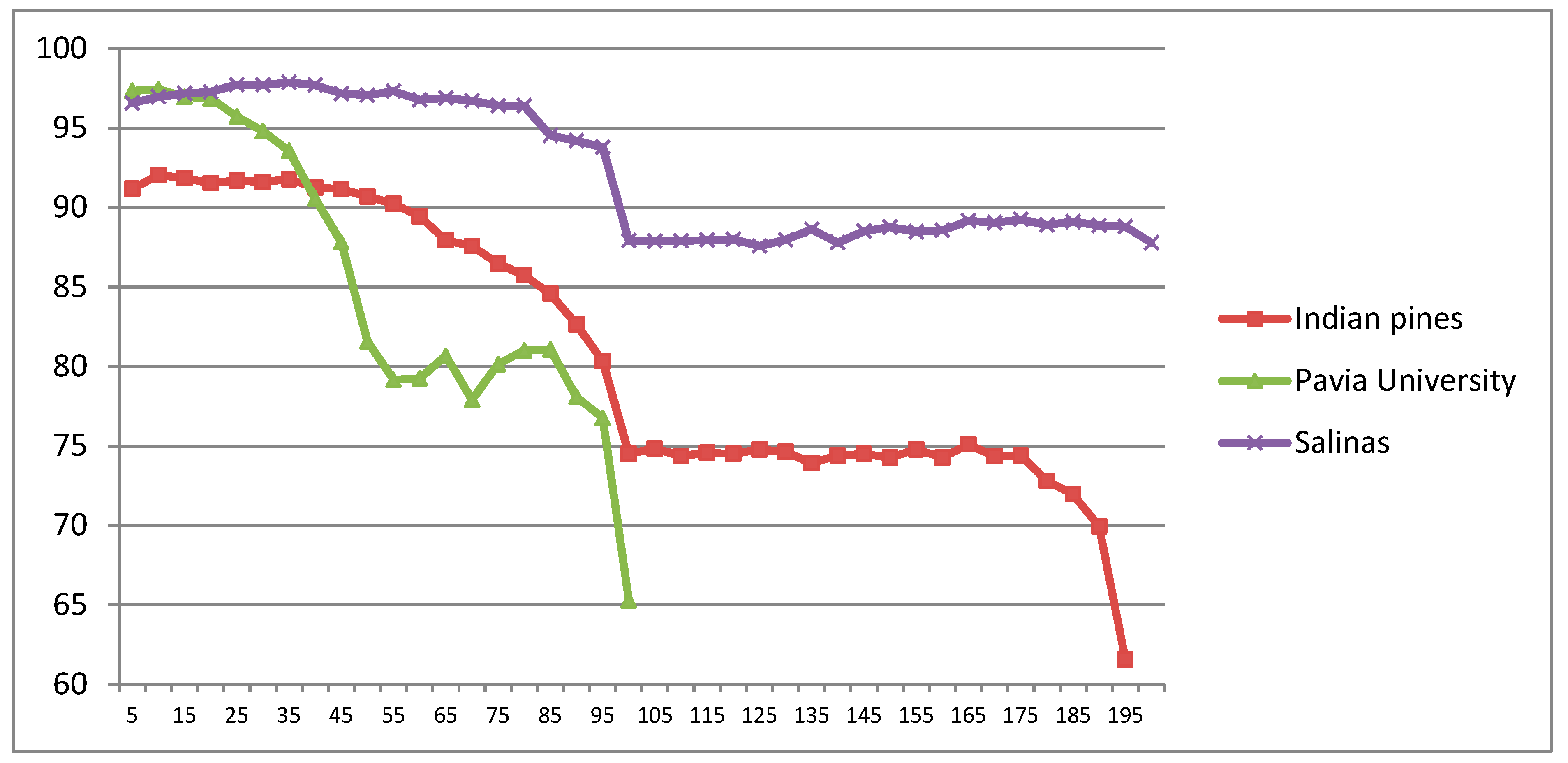
The count of the retained coefficients after performing the spectral DCT represents the spectral filter parameter. This parameter is set by comparing the classification accuracy OA with varying numbers of DCT coefficients where the count of the retained coefficients corresponds to the most accurate classification OA for each dataset. Figure 7 illustrates the classification accuracies in terms of OA for the CDCT-2DCT_SVM framework with a different number of DCT coefficients on the Indian Pines, Salinas, and Pavia University datasets.
As shown in Figure 7, it is clear that the classification accuracy OA is the the highest when incorporating up to ten first coefficients for the three datasets. Classification accuracy decreases due to the influence of noise present in the high-frequency components when selecting more than 40, 70, and 20 coefficients for the Indian Pines, Salinas, and Pavia University datasets, respectively. In our experiments, therefore, only ten DCT coefficients were retained for the three datasets. For each dataset, ten DCT coefficient were also set in the other methods used for comparison, based on performing a spectral DCT including DCT_SVM, SDCT-2DCT_SVM, and S2DCT-DCT_SVM.
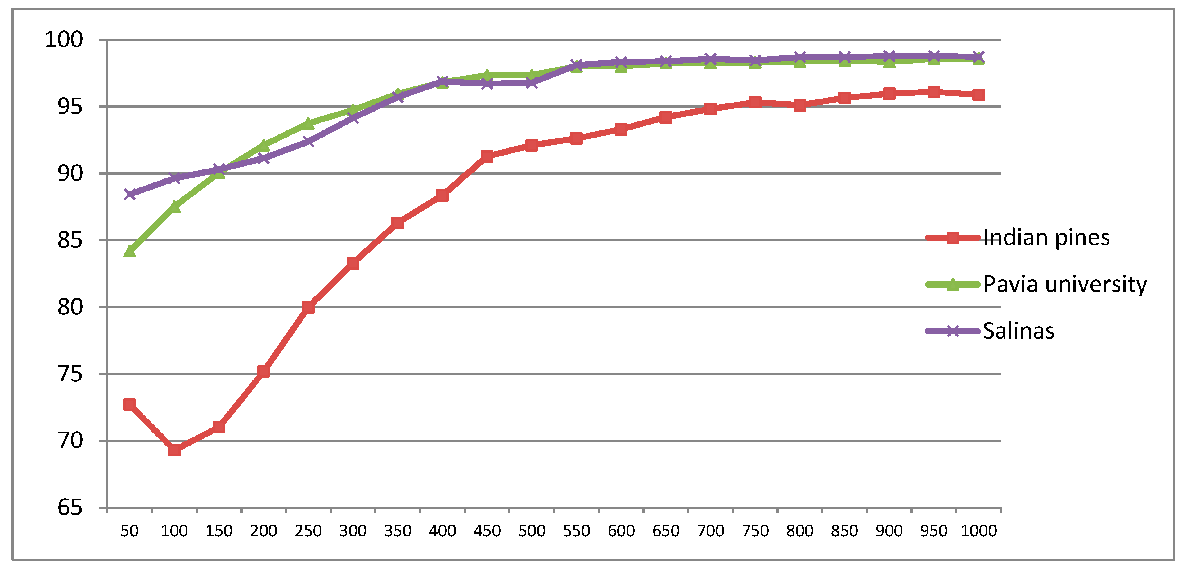
The spatial filter parameter in the CSDCT-2DCT_SVM approach was the threshold for 2D-DCT. This parameter was set by comparing the classification accuracy OA with varying threshold values where the opted threshold corresponds to the best classification OA for each dataset. Figure 8 depicts the variation of the classification accuracy OA with varying threshold values, ranging from 50 to 1000 with the step of 50, on Indian Pines, Salinas, and Pavia University datasets.
As can be seen in Figure 8, the OA increased with a higher threshold value for all datasets and tend to be stable around the threshold of 500 for Indian Pines, while this degree of stability was obtained at around a threshold of 450 for Salinas and Pavia University datasets. Therefore, a maximum threshold of 500was selected for the three datasets in our experiments. This threshold value is also selected in the other compared methods based on using 2D-DCT, including 2DCT_SVM, S2DCT-DCT_SVM, and SDCT-2DCT_SVM. The parameter settings of the CDCT-WF_SVM framework are explained in the next subsection.

5.1.2. CDCT-WF_SVM Framework Parameter Estimation

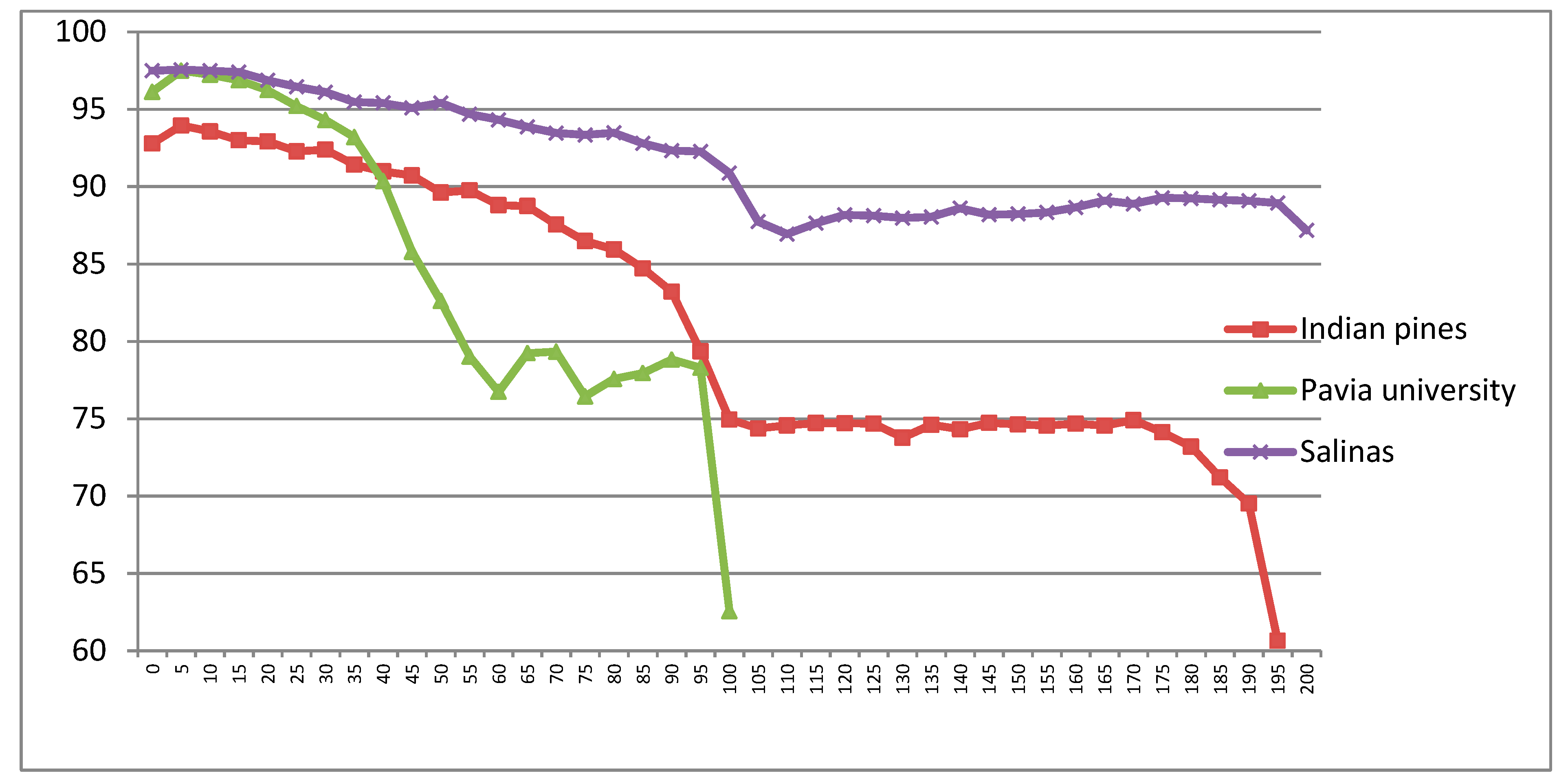
The spectral filter parameter in this approach is the count of the retained coefficients after performing the spectral DCT, estimated in the same way as in the first approach. Thus, this parameter was set by comparing the classification accuracy OA with varying number of DCT coefficients where the count of the retained coefficients corresponds to the most accurate classification OA for each dataset. Figure 9 illustrates the classification accuracies in terms of OA for the CDCT-WF_SVM framework with a different number of DCT coefficients on Indian Pines, Salinas, and Pavia University datasets.
As shown in Figure 9, for the CDCT-WF_SVMapproach, the classification accuracy OA was maximal when incorporating the five first coefficients for the three datasets. Also, the OA decreased due to the influence of noise present in the high-frequency components when selecting more than 15 coefficients for the three datasets. In our experiments, therefore, only five DCT coefficients were retained for the three dataset.
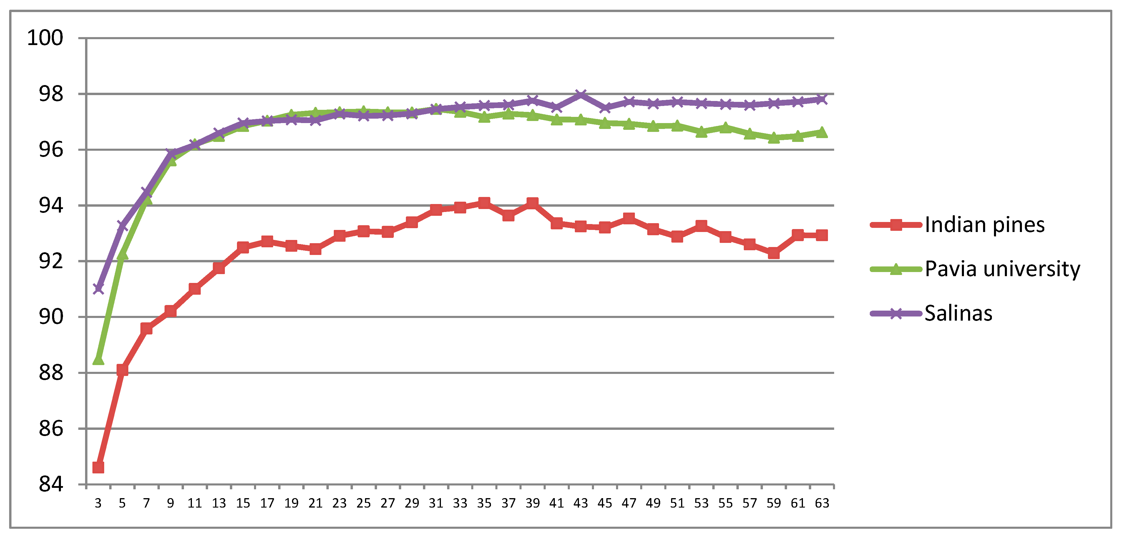
Wiener filter patch size represents the spatial parameter in the CSDCT-WF_SVM approach. This parameter was set by comparing the classification accuracy OA with varying Wiener filter patch sizes where the opted patch size corresponds to the best classification OA for each dataset. Figure 10 depicts the variation of the classification accuracy OA with varying filter patch sizes, ranging from 3 × 3 to 63 × 63 pixels, on Indian Pines, Salinas, and Pavia University datasets.
As can be seen in Figure 10, classification accuracy (OA) increased with a larger patch size value for the three datasets. Thus, accuracies tend to become stable at around a 39 × 39 patch size for the Indian Pines dataset, at around 43 × 43 patch size for Salina dataset, and a 31 × 31 patch size for Pavia University dataset. Therefore, these patch sizes were selected for our experiments corresponding to each dataset.
The summary of the important parameters involved in our experiments on different datasets is given in Table 5.

5.2. Classification of Indian Pines Dataset

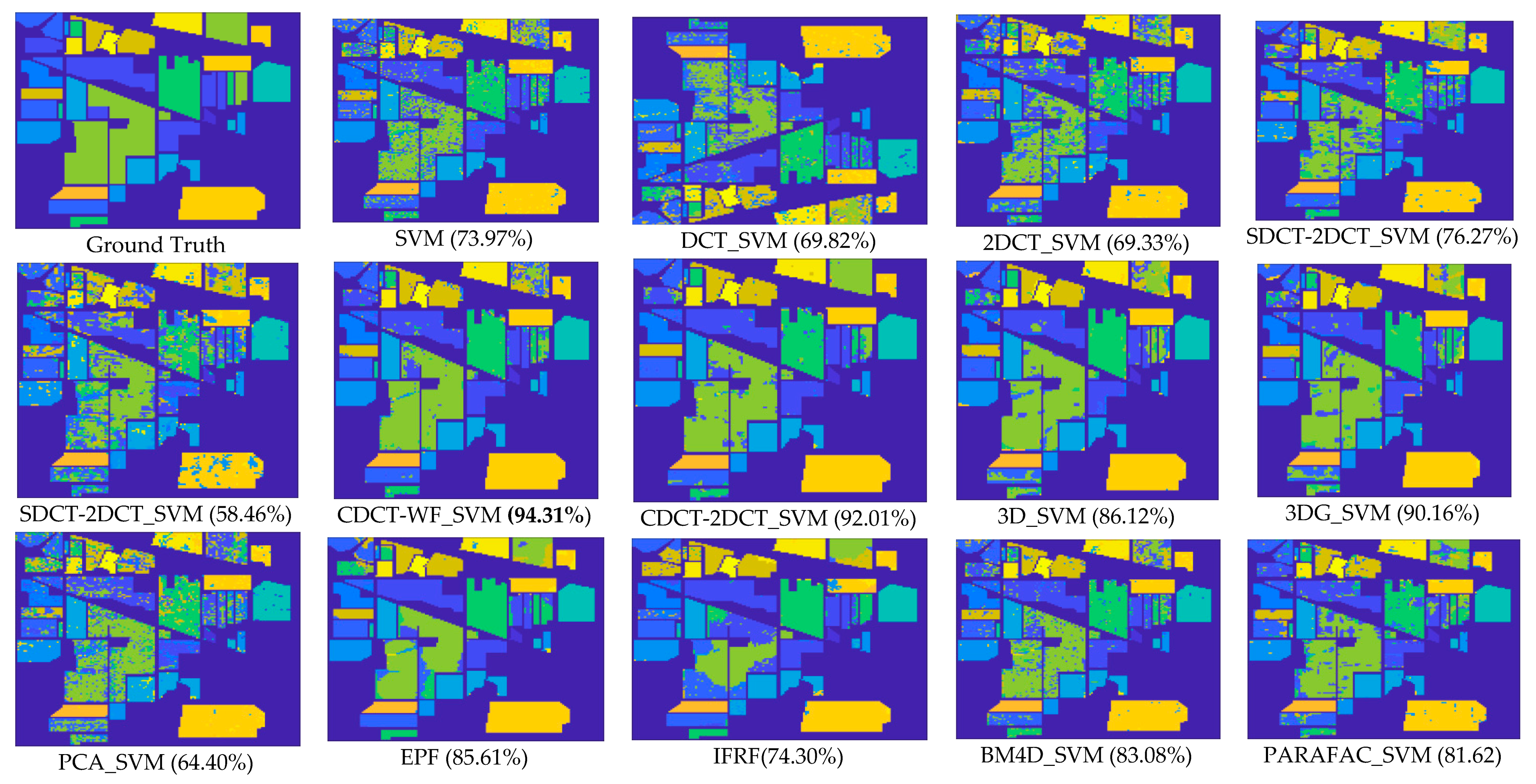
In this subsection, we compare the classification effectiveness of the proposed frameworks CDCT-2DCT_SVM and CDCT-WF_SVM with the other classification methods on the Indian Pines dataset. The first experiment assessed the validity of our proposed approaches relative to the other methods. The results reported in Table 6 represent the averages of the individual classification accuracies (%), κ statistic, standard deviation, AA, OA, and computational time in seconds. Classification maps for all the compared approaches are shown in Figure 11.
Figure 11 and Table 6 show that CDCT-WF_SVM achieved the highest values for the three criteria (AA, OA, and κ), followed by CDCT_2DCT_SVM, which had the second best performance (94.31% OA and 92.01% OA, respectively). The classification maps produced with both the CDCT-WF_SVM and CDCT-2DCT_SVM approaches are smooth and close to the ground truth map, as shown in Figure 11.
Several observations can also be made:
-
The approaches exploring only the spectral information, including SVM, PCA_SVM, and SDCT_SVM, attain poorer results when compared with the other techniques, which can be confirmed in Figure 11, where it is clear that the classification maps resulted from these techniques are degraded by salt-and-pepper noise. Nevertheless, the classification accuracy of SDCT_SVM (73.07% OA) is higher than PCA_SVM (64.40% OA) owing to the effectiveness ofDCT energy compaction that concentrates the energy of the spectral signature in a few low-frequency components where noisy data is embedded in the high-frequency components; instead of selecting the first PCs in PCA which cannot guarantee that image quality decreases for PCs with lower variances. The 2D-DCT_SVM approach only filters spatial information and therefore yielded less accurate results.
-
The methods considering both the spectral and spatial information, including 3DG_SVM, 3D_SVM, EPF, IFRF, BM4D_SVM, and PARAFAC_SVM, are most accurate. The 3DG_SVM, and_3DSV methods delivered the third and fourth highest accuracies (90.32% OA and 86.12% OA, respectively) given the efficiency of wavelet features in structural filtering. Nevertheless, by considering hyperspectral image data as a 3D cube where the spatial and spectral features must be treated as a whole in 3D-DWT approaches, we implicitly assume that the noise variance is the same in the three dimensions and ignores dissimilarity between the spatial and the spectral dimensions where the degree of irregularity is higher in the spectral dimension than in the spatial dimensions. The proposed CDCT-WF_SVM and CDCT-2DCT_SVM approaches overcome this issue by filtering the spectral dimension and the spatial dimensions separately to achieve higher performance than wavelet-based filtering approaches. Moreover, the highest accuracy (94.31% OA) was achieved by CDCT-WF_SVM, which combines two different filters and take advantage of both of them. Additionally, it can be seen in Figure 11 that 3D_SVM, 3DG_SVM, EPF, and IFRF achieved smoother classification maps than the two well-known denoising-based approaches, BM4D_SVM and PARAFAC_SVM.
-
Serial filtering-based approaches including SDCT-2DCT_SVM and S2DCT-DCT_SVM obtained by performing spectral and spatial filters on the same information cannot be effective in improving the classification accuracy, since performing a second filter on the already filtered information will alter the useful information rather than discarding more noise. In contrast, the proposed CDCT-WF_SVM and CDCT-2DCT_SVM perform a spatial filter on the noisy part from the spectral filter.
-
Regarding the computational cost, Table 6 shows that the shortest classification time was 1.48 s and was achieved with the IFRF method, which had low classification accuracy (74.30% OA). The other spectral-spatial-based methods including EPF (85.61%OA), 3D_SVM (86.12%OA), 3DG_VM ((90.32%OA) achieved higher classification accuracies, but they are time-consuming using 85.61s, 86.12s, and 210.16s, respectively. Similarly, denoising-based techniques are also time-consuming with 83.08s for BM4D_SVM and 81.62 for PARAFAC_SVM. However, the proposed CDCT-WF_SVM and CDCT-2DCT_SVM achieved the two first highest classification accuracies within a short execution time. For example, CDCT-WF_SVM achieved an OA of 94.31% in 13.30s where CDCT-2DCT_SVM achieves an OA of 92.01% in 13.91s. Moreover, in the proposed approaches, the SDCT is performed on each pixel, and the spatial filter is performed on each band. Hence, our approaches are easily parallelized, which could further reduce the computational time.
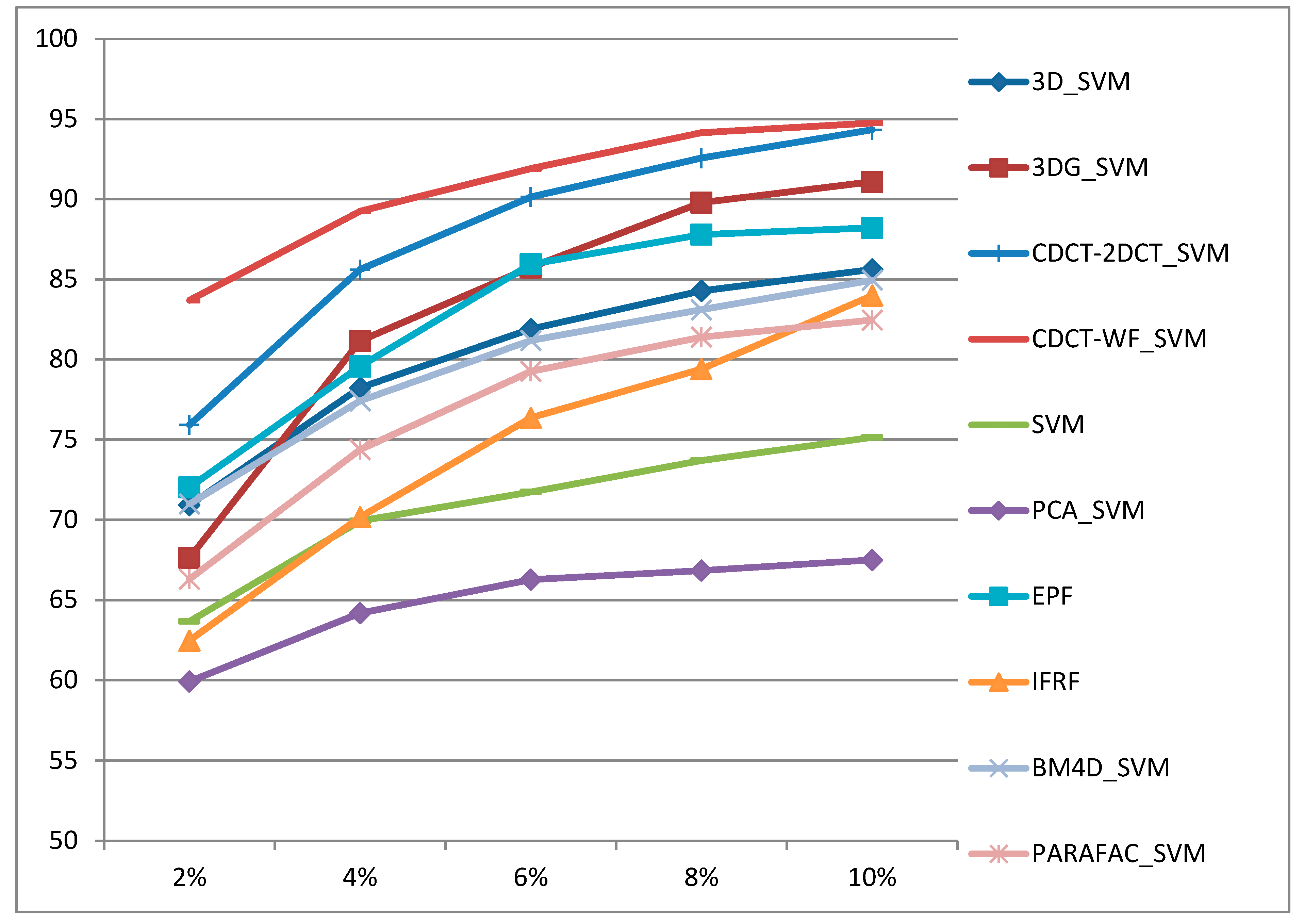
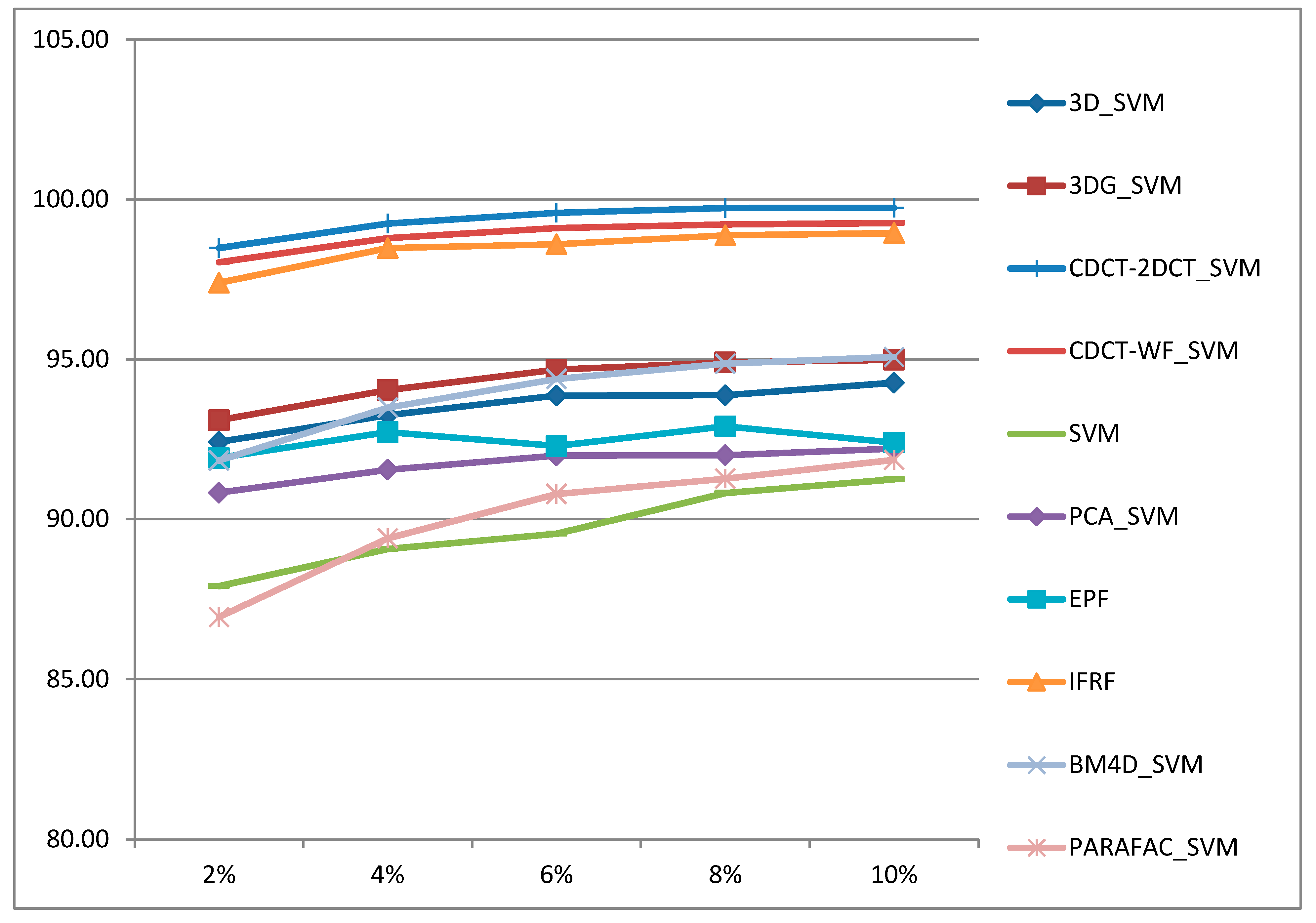
The performance of the classifiers is greatly affected by the number of training samples. Therefore, in our second experiment, the performance of the proposed frameworks was evaluated against state-of-the-art approaches under different training conditions, in which 2%, 4%, 6%, 8%, and 10% labeled samples of each class are randomly selected as training samples, while the rest are used as test samples. Each experiment was performed 20 times and the average results in terms of the OA values for each method are plotted in Figure 12.
Figure 12 illustrates that the proposed frameworks can significantly improve classification results when varying the training samples size, as the size of training samples changes from 2% to 10%, our proposed approaches (CDCT-WF_SVM and CDCT-2DCT_SVM) always achieved the first and the second highest OA. Their advantages are apparent from the small size of the training samples. The proposed CDCT-WF_SVM has an 11.67–23.78% gain in accuracy over the other tested compared methods with a 2% training sample per class. This indicates that a large number of unlabeled samples can be discerned with a small labeled samples size, which further demonstrates the robustness of the proposed approaches.

5.3. Classification of SALINAS Dataset

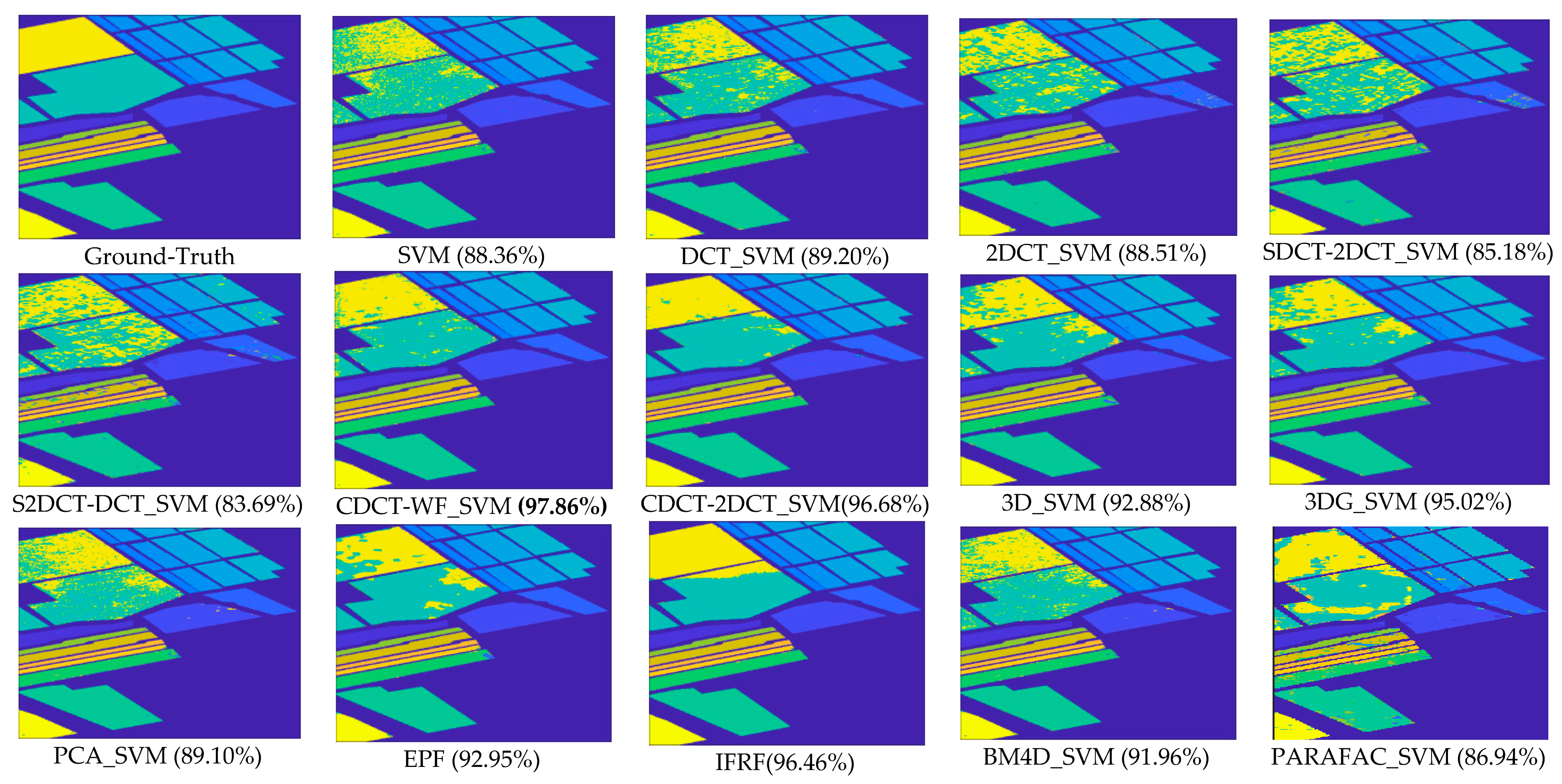
In the first experiment, we compared our proposed approaches and other methods on the Salinas dataset. Table 7 reports the quantitative classification results including the individual classification accuracies (%), κ statistic, standard deviation, AA, OA, and computational time in seconds. The classification maps for all the compared approaches on Salinas scene are illustrated in Figure 13.
From Table 7, we can see that our proposed CDCT-WF_SVM approach provided the highest classification accuracy in terms of all the three criteria (AA, OA, and kappa), with stable performance (lower standard deviation). Hence, it achieved the highest classification accuracy in terms of OA (97.86%). Our proposed CDCT-2DCT_SVM method provided the second highest classification with an OA of 96.68%. In addition, the classification maps produced from both the CDCT-WF_SVM and CDCT-2DCT_SVM approaches are smooth and close to the ground truth map, as shown in Figure 13. From Table 7, it is clear that IFRF (96.46%OA) produced more accurate classification results than 3DG_SVM (83.34%OA) in this scenario, with much smoother classification map. The EPF, 3D_SVM and BM4D_SVM methods achieved comparable classification OA values (92.95%, 92.88% and 91.96%, respectively), resulting in similar classification maps, as shown in Figure 13. The PARAFAC_SVM method delivers lower classification accuracy (86.94%OA) than the pixel-wise classifiers including DCT_SVM, PCA_SVM, 2DCT_SVM, and SVM. Also, the two approaches based on serial filtering, SDCT-2DCT_SVM and S2DCT-DCT_SVM yielded low classification OA values (88.51%, and 83.69%, respectively).This is likely because the second filter altered the meaningful information that had been filtered by the first filter already.
Table 7 shows that classifiers with spatial information cost more time than their pixel-wise counterparts. Meanwhile, the IFRF, which is a spectral-spatial feature extraction-based method, achieves the shortest time of 4.77 s. Our proposed CDCT-WF_SVM approach achieved the third least execution time with 61.22 s among the spectral-spatial classifiers after IFRF and EPF (19.02 s) methods. From Table 7, we can also conclude that wavelet-based and denoising approaches are time-consuming. For example, 3DG_SVM requires 1142.52 s to achieve an OA of 95.02% where our proposed CDCT-WF_SVM approach requires only 65.22 s to achieve an OA of 97.86%, and the proposed CDCT-2DCT_SVM requires 70.56 s to provide an OA of 96.68%.
In the second experiment, the robustness of the proposed approaches regarding the state-of-the-art methods with different training conditions was evaluated, in which 2%, 4%, 6%, 8%, and 10% labeled samples of each class were randomly selected as training samples, while the rest are used as testing samples. Thus, for stability, each experiment was executed 20 times, and the averages result in terms of the OA values are plotted in Figure 14.
Figure 14 shows that the proposed frameworks can always improve the classification accuracy with a different number of training samples, as the number of training samples varies from 2% to 10%, our proposed approaches (CDCT-2DCT_SVM and CDCT-WF_SVM) always achieved the first and the second highest OA. Additionally, it should be noted that the IFRF method had the third-highest accuracy when varying the number of training samples and outperforms wavelet-based approaches (3DG_SVM and 3D_SVM).

5.4. Classification of Pavia University Dataset

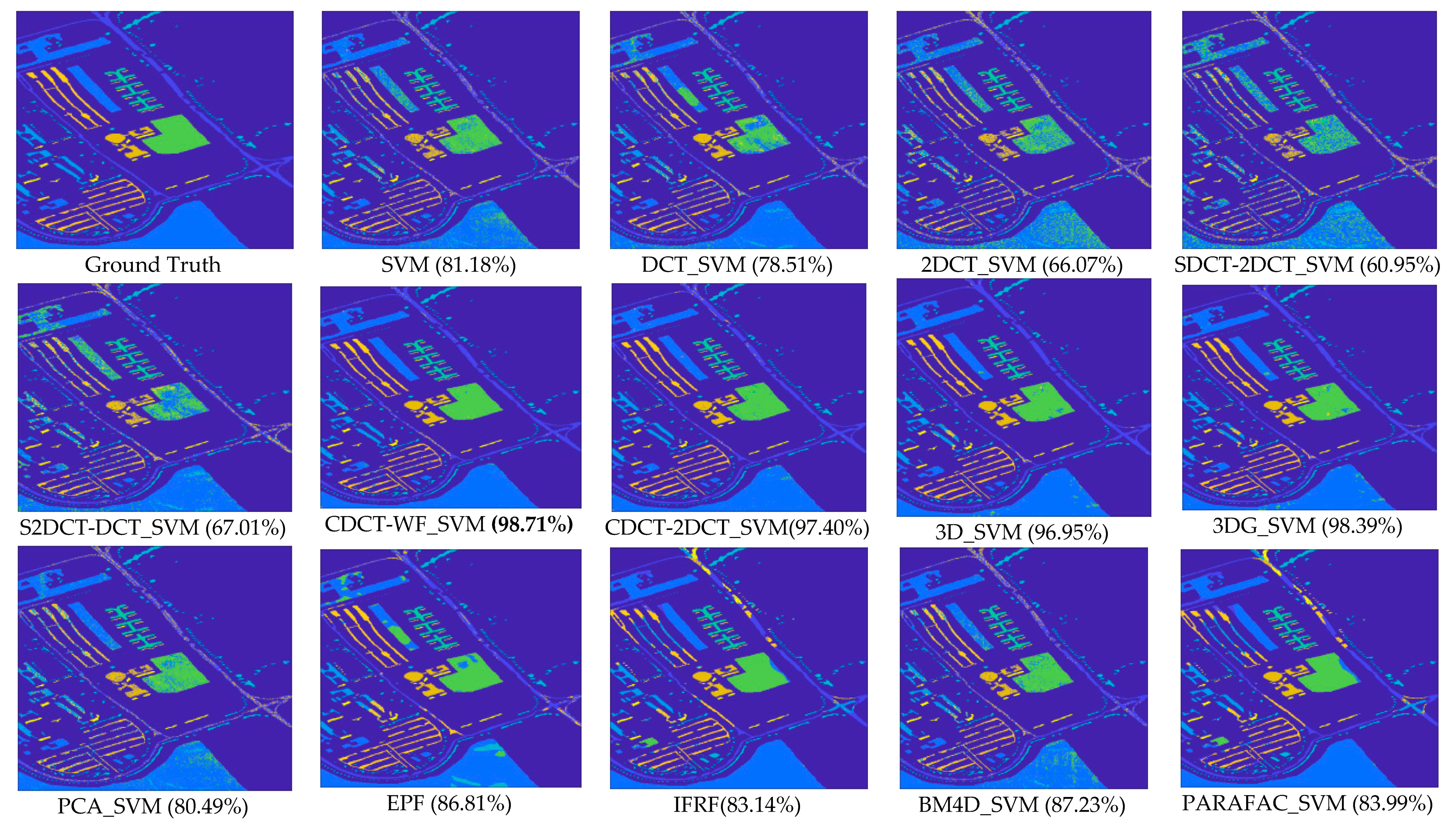
In the first experiment, we compare the classification effectiveness of the proposed frameworks with the other classification methods on Pavia University dataset. Table 8 reports the quantitative classification results. Details of the classification maps of the compared approaches are shown in Figure 15.
As can be seen in Table 8, the highest classification accuracies are always obtained by the spectral-spatial classification techniques, especially the structural filtering-based approaches. The proposed method CDCT-WF_SVM achieved the highest accuracy. For example, the OA obtained by this approach was around 98.71%, which is 17.53% higher than OA obtained by the pixel-wise SVM classifier.
In this scene, 3DG_SVM provides competitive performance, which is 98.39% in terms of OA followed by our proposed CDCT-2DCT_SVM approach with an OA of 97.40% and the 3D_SVM method with an OA of 96.95%. Although the structural filtering approaches have comparable accuracy, the processing time of our proposed frameworks is faster than wavelet-based methods. For example, the proposed CDCT-WF_SVM achieve an OA of 98.71% in 124.93 s, where 3DG_SVM achieved an OA of 98.39% in 2142.40 s, which is 17 times slower than our proposed CDCT-WF_SVM approach. Another observation is that BM4D_SVM and EPF methods achieve comparable classification OA (87.23% and 86.81%, respectively). Meanwhile, PARAFAC_SVM and IFRF were the least accurate among the spectral-spatial classifiers, with an OA of 83.99% and 83.14%, respectively. The pixel-wise classifiers including SVM, PCA_SVM, and DCT_SVM methods produced the least accurate classification results. For example, the OA values were 81,18%, 80,49%, and 78.51%, respectively. Similar to the experiments with other datasets, serial filtering-based approaches yielded the least accurate classification results.
From Figure 15, we can see visually that combining spectral and spatial information produce less noisy and smoother results. In particular, structural filtering-based approaches have smoother classification maps than the other methods. The results obtained from our proposed CDCT-WF_SVM approach closely match the ground-truth map.
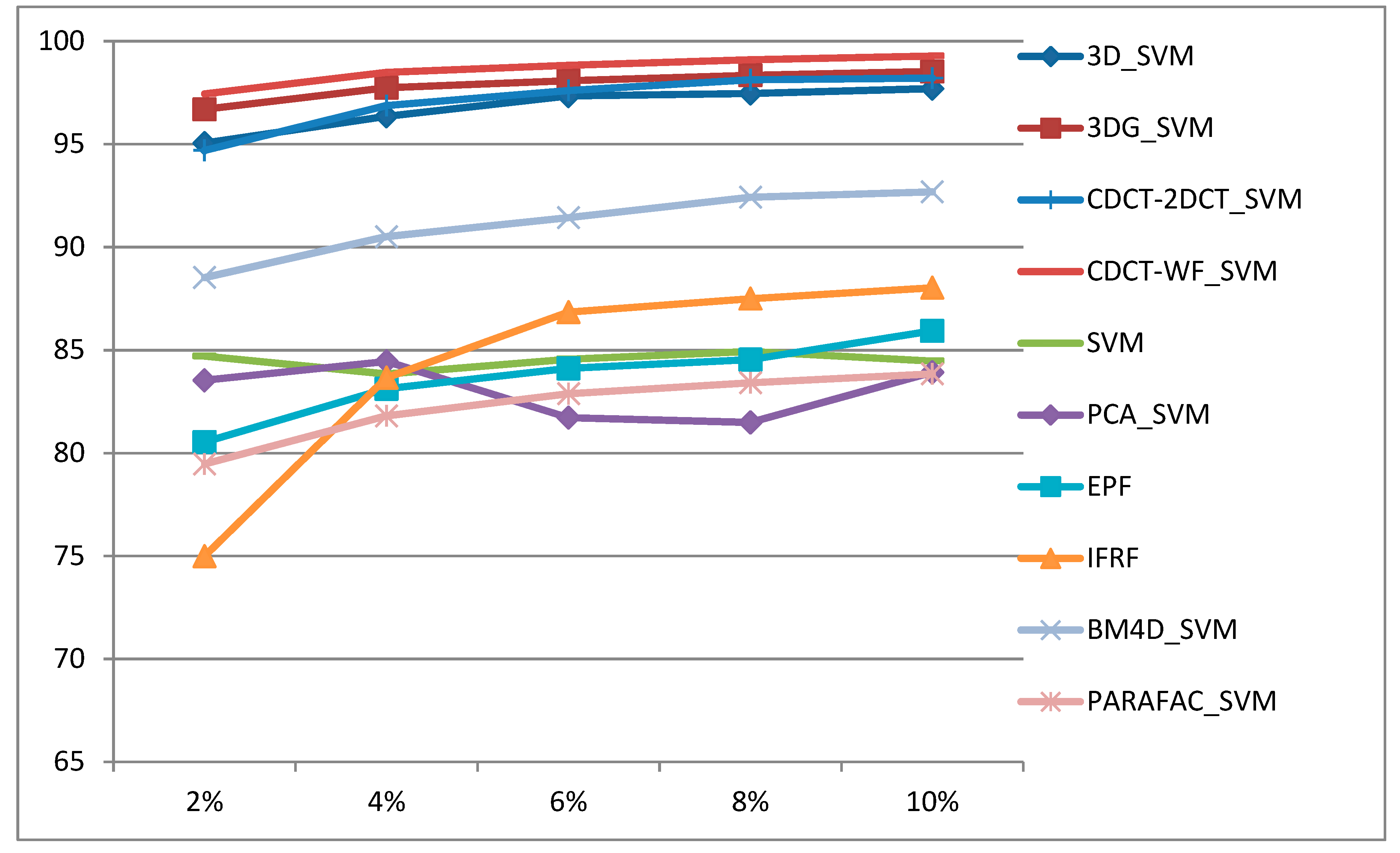
In the second experiment, we evaluated the performance of the proposed frameworks on Pavia University image against state-of-the-art methods with different training conditions, in which 2%, 4%, 6%, 8%, and 10% labeled samples of each class are randomly selected as training samples, and the rest are used for testing. The averages results in terms of OA values for each compared method are plotted in Figure 16.
Figure 16 illustrates that the proposed frameworks can always improve the classification accuracy significantly with a different number of training samples, as the size of training samples changes from 2% to 10%, the proposed approach (CDCT-WF_SVM) always achieved the first highest OA followed by 3DG_SVM, CDCT-2DCT_SVM, and 3D_SVM, which have a comparable performance when varying the size of training samples. Meanwhile, it should be noted that BM4D_SVM provided higher accuracy than EPF and IFRF methods when varying the training samples size.

5.5. Classification in Noisy Scenario

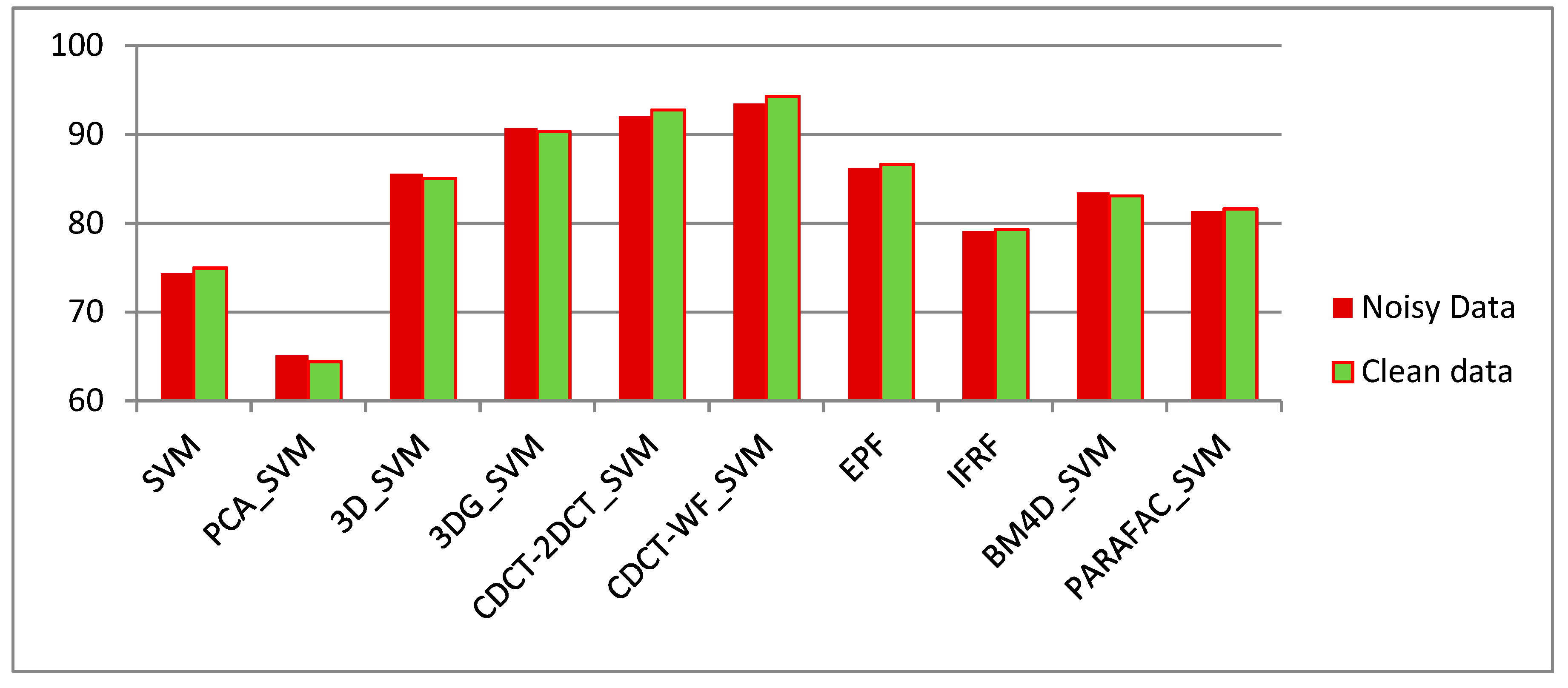
In the noisy scenario experiment, we evaluated the robustness of our proposed approaches on the Indian Pines dataset with all 224 spectral bands without removing the 24 noisy bands as done in the former experiment. This noisy Indian pines dataset is publicly available at http://www.ehu.eus/ccwintco/index.php/Hyperspectral_Remote_Sensing_Scenes. As in the experiment on the clean Indian Pines dataset discussed in Section 5.2, we randomly chose 100 samples for each class from the reference data as training samples, and the rest were used as test samples as given in Table 1. The classification accuracy OA of all the state-of-the-art methods with the clean Indian Pines dataset (with only 200 bands) and the noisy Indian Pines dataset (224 bands including the 24 noisy bands) are compared in Figure 17.
From Figure 17, although the classification accuracy of all the compared methods on the noisy scenario was lower than on the clean dataset, nevertheless, the proposed CDCT-WF_SVM and CDCT-2DCT_SVM still provided a higher OA than the other methods in this noisy scenario, which further shows the robustness of our proposed approaches in the noisy scenario relative to the other tested methods. Another observation is that denoising-based approaches including BM4D_SVM and PARAFAC_SVM methods, achieved comparable classification OA on both clean and noisy scenarios. Meanwhile, PCA_SVM was the least accurate among all compared methods. This is because PCA is a global transformation and neither maintains the local spectral signatures nor considers noise. Consequently, it might not preserve all the required useful information for providing effective and reliable classification [71].

6. Summary and Conclusions

In this paper, we present two effective classification frameworks based on cascaded spectral and spatial filtering where the spatial filter is performed in the DCT domain. In our proposed frameworks, we perform a spectral DCT to separate the most significant information presented in a few low-frequency components from the noisy data embedded in high-frequency components. Spatial filtering exploiting both 2D-DCT and WF are performed on the high DCT frequency components to extract the rest of useful spatial information. After applying an inverse DCT on all components, including the filtered components, the linear SVM classifier was applied to the preprocessed data. Various performance metrics were used to support our experimental studies including the classification accuracy, computational time, the classification maps, and the sensitivity tests for different sizes of the training samples. Experimental results on three real hyperspectral datasets show that our approaches outperform the state-of-the-art methods investigated in this paper. The most significant results of this work are listed below:
-
The proposed approaches outperform the other considered methods; in particular, our proposed CDCT-WF_SVM method, which delivers higher accuracy on the three datasets with a smoother classification map than the other tested techniques.
-
The proposed approaches deliver higher classification accuracies regardless of the size of training samples, and they are robust to noise.
-
A major advantage of the proposed frameworks is that they are computationally efficient along with a reasonable tradeoff between accuracy and computational time. Thus, they will be quite useful for applications such as flood monitoring and risk management, which require a fast response. Moreover, as the DCT is performed on each pixel, and both WF with 2D-DCT are performed on each band, our approaches are easily parallelized, which could further reduce the computational time.
-
The results obtained illustrate that the proposed approaches can deal with different spatial resolutions (20 m, 3.7 m, and 1.7 m). In particular, for Indian pines dataset with 20m spatial resolution, our proposed CDCT-WF_SVM and CDCT-2DCT_SVM approaches achieve first and the second highest accuracy. Thus, our proposed approaches can effectively deal with low spatial resolution images.
-
For the three datasets, structural-based filtering methods have stable performance, including our proposed frameworks and wavelet-based methods. However, the IFRF method cannot provide stable performance by providing the third-highest accuracy on Salinas dataset and low accuracy on the two other datasets.
-
The proposed approaches require the selection of only two parameters to achieve high classification accuracy in low computational time, which allows their potential use in practical applications.

Author Contributions

All authors have made great contributions to the work. Conceptualization, R.B. and K.B.; Software, R.B. and K.B.; validation, W.H., R.B. and K.B.; formal analysis, R.B.; supervision, H.W., Writing—original draft, R.B.; and Writing—review and editing, H.W. and K.B.

Funding

This research received no external funding.

Acknowledgments

The authors are grateful for the valuable comments and propositions from the reviewer of this paper.

Conflicts of Interest

The authors declare no conflict of interest.

References

  1. Tong, Q.; Xue, Y.; Zhang, L. Progress in Hyperspectral Remote Sensing Science and Technology in China Over the Past Three Decades. IEEE J. Sel. Top. Appl. Earth Obs. Remote Sens. 2014, 7, 70–91. [Google Scholar] [CrossRef]
  2. Adão, T.; Hruška, J.; Pádua, L.; Bessa, J.; Peres, E.; Morais, R.; Sousa, J.J. Hyperspectral Imaging: A Review on UAV-Based Sensors, Data Processing and Applications for Agriculture and Forestry. Remote Sens. 2017, 9, 1110. [Google Scholar] [CrossRef]
  3. Yokoya, N.; Chan, J.C.-W.; Segl, K. Potential of Resolution-Enhanced Hyperspectral Data for Mineral Mapping Using Simulated EnMAP and Sentinel-2 Images. Remote Sens. 2016, 8, 172. [Google Scholar] [CrossRef]
  4. He, J.; He, Y.; Zhang, A.C. Determination and Visualization of Peimine and Peiminine Content in Fritillaria thunbergii Bulbi Treated by Sulfur Fumigation Using Hyperspectral Imaging with Chemometrics. Molecules 2017, 22, 1402. [Google Scholar] [CrossRef]
  5. Melgani, F.; Bruzzone, L. Classification of hyperspectral remote sensing images with support vector machines. IEEE Trans. Geosci. Remote Sens. 2004, 42, 1778–1790. [Google Scholar] [CrossRef] [Green Version]
  6. Ham, J.; Chen, Y.; Crawford, M.M.; Ghosh, J. Investigation of the random forest framework for classification of hyperspectral data. IEEE Trans. Geosci. Remote Sens. 2005, 43, 492. [Google Scholar] [CrossRef]
  7. Ratle, F.; Camps-Valls, G.; Weston, J. Semisupervised neural networks for efficient hyperspectral image classification. IEEE Trans. Geosci. Remote Sens. 2010, 48, 2271–2282. [Google Scholar] [CrossRef]
  8. Zhong, Y.; Zhang, L. An adaptive artificial immune network for supervised classification of multi-/hyperspectral remote sensing imagery. IEEE Trans. Geosci. Remote Sens. 2012, 50, 894–909. [Google Scholar] [CrossRef]
  9. Chen, Y.; Nasrabadi, N.M.; Tran, T.D. Hyperspectral Image Classification via Kernel Sparse Representation. IEEE Trans. Geosci. Remote Sens. 2013, 51, 217–231. [Google Scholar] [CrossRef]
  10. Castrodad, A.; Xing, Z.; Greer, J.B.; Bosch, E.; Carin, L.; Sapiro, G. Learning Discriminative Sparse Representations for Modeling, Source Separation, and Mapping of Hyperspectral Imagery. IEEE Trans. Geosci. Remote Sens. 2011, 49, 4263–4281. [Google Scholar] [CrossRef]
  11. Li, J.; Bioucas-Dias, J.M.; Plaza, A. Spectral-spatial classification of hyperspectral data using loopy belief propagation and active learning. IEEE Trans. Geosci. Remote Sens. 2013, 51, 844–856. [Google Scholar] [CrossRef]
  12. Di, W.; Crawford, M.M. View generation for multiview maximum disagreement based active learning for hyperspectral image classification. IEEE Trans. Geosci. Remote Sens. 2012, 50, 1942–1954. [Google Scholar] [CrossRef]
  13. Wang, Y.; Duan, H. Classification of Hyperspectral Images by SVM Using a Composite Kernel by Employing Spectral, Spatial and Hierarchical Structure Information. Remote Sens. 2018, 10, 441. [Google Scholar] [CrossRef]
  14. Camps-Valls, G.; Tuia, D.; Bruzzone, L.; Benediktsson, J.A. Advances in hyperspectral image classification: Earth monitoring with statistical learning methods. IEEE Signal Process. Mag. 2014, 31, 45–54. [Google Scholar] [CrossRef]
  15. Plaza, A.; Benediktsson, J.A.; Boardman, J.W.; Brazile, J.; Bruzzone, L.; Camps-Valls, G.; Chanussot, J.; Fauvel, M.; Gamba, P.; Gualtieri, A.; et al. Recent advances in techniques for hyperspectral image processing. Remote Sens. Environ. 2009, 113, S110–S122. [Google Scholar] [CrossRef]
  16. He, L.; Li, J.; Liu, C.; Li, S. Recent advances on spectral-spatial hyperspectral image classification: An overview and new guidelines. IEEE Trans. Geosci. Remote Sens. 2018, 56, 1579–1597. [Google Scholar] [CrossRef]
  17. Plaza, A.; Martinez, P.; Plaza, J.; Perez, R. Dimensionality reduction and classification of hyperspectral image data using sequences of extended morphological transformations. IEEE Trans. Geosci. Remote Sens. 2005, 43, 466. [Google Scholar] [CrossRef]
  18. Benediktsson, J.A.; Palmason, J.A.; Sveinsson, J.R. Classification of Hyperspectral Data from Urban Areas Based on Extended Morphological Profiles. IEEE Trans. Geosci. Remote Sens. 2005, 43, 480. [Google Scholar] [CrossRef]
  19. Xia, J.; Chanussot, J.; Du, P.; He, X. Spectral-spatial classification for hyperspectral data using rotation forests with local feature extraction and Markov random fields. IEEE Trans. Geosci. Remote Sens. 2015, 53, 2532–2546. [Google Scholar] [CrossRef]
  20. Khodadadzadeh, M.; Li, J.; Plaza, A.; Ghassemian, H.; Bioucas-Dias, J.M.; Li, X. Spectral–Spatial Classification of Hyperspectral Data Using Local and Global Probabilities for Mixed Pixel Characterization. IEEE Trans. Geosci. Remote Sens. 2014, 52, 6298. [Google Scholar] [CrossRef]
  21. Peng, J.; Zhou, Y.; Chen, C.L.P. Region-kernel-based support vector machines for hyperspectral image classification. IEEE Trans. Geosci. Remote Sens. 2015, 53, 4810–4824. [Google Scholar] [CrossRef]
  22. Chen, Y.; Nasrabadi, N.M.; Tran, T.D. Hyperspectral Image Classification Using Dictionary-Based Sparse Representation. IEEE Trans. Geosci. Remote Sens. 2011, 49, 3973. [Google Scholar] [CrossRef]
  23. Lu, Z.; He, J. Spectral-spatial hyperspectral image classification with adaptive mean filter and jump regression detection. Electron. Lett. 2015, 51, 1658–1660. [Google Scholar] [CrossRef]
  24. Golipour, M.; Ghassemian, H.; Mirzapour, F. Integrating Hierarchical Segmentation Maps with MRF Prior for Classification of Hyperspectral Images in a Bayesian Framework. IEEE Trans. Geosci. Remote Sens. 2016, 54, 805. [Google Scholar] [CrossRef]
  25. Oktem, R.; Ponomarenko, N.N. Image filtering based on discrete cosine transform. Telecommun. Radio Eng. 2007, 66. [Google Scholar] [CrossRef]
  26. Guo, X.; Huang, X.; Zhang, L. Three-Dimensional Wavelet Texture Feature Extraction and Classification for Multi/Hyperspectral Imagery. IEEE Geosci. Remote Sens. Lett. 2014, 11, 2183. [Google Scholar]
  27. Sun, S.; Zhong, P.; Xiao, H.; Wang, R. An MRF model-based active learning framework for the spectral-spatial classification of hyperspectral imagery. IEEE J. Sel. Top. Signal Process. 2015, 9, 1074–1088. [Google Scholar] [CrossRef]
  28. Li, W.; Prasad, S.; Fowler, J.E. Hyperspectral image classification using Gaussian mixture models and Markov random fields. IEEE Geosci. Remote Sens. Lett. 2014, 11, 153–157. [Google Scholar] [CrossRef]
  29. Ghamisi, P.; Benediktsson, J.A.; Cavallaro, G.; Plaza, A. Automatic Framework for Spectral–Spatial Classification Based on Supervised Feature Extraction and Morphological Attribute Profiles. IEEE J. Sel. Top. Appl. Earth Obs. Remote Sens. 2014, 7, 2147. [Google Scholar] [CrossRef]
  30. Gu, Y.; Liu, T.; Jia, X.; Benediktsson, J.A.; Chanussot, J. Nonlinear multiple kernel learning with multiple-structure-element extended morphological profiles for hyperspectral image classification. IEEE Trans. Geosci. Remote Sens. 2016, 54, 3235–3247. [Google Scholar] [CrossRef]
  31. Pan, B.; Shi, Z.; Xu, X. R-VCANet: a new deep-learning-based hyperspectral image classification method. IEEE J. Sel. Top. Appl. Earth Obs. Remote Sens. 2017, 10, 1975–1986. [Google Scholar] [CrossRef]
  32. Pan, B.; Shi, Z.; Xu, X. MugNet: deep learning for hyperspectral image classification using limited samples. ISPRS J. Photogramm. Remote Sens. 2017. [Google Scholar] [CrossRef]
  33. Pan, B.; Shi, Z.; Xu, X. Hierarchical guidance filtering-based ensemble classification for hyperspectral images. IEEE Trans. Geosci. Remote Sens. 2017, 55, 4177–4189. [Google Scholar] [CrossRef]
  34. Ni, D.; Ma, H. Hyperspectral image classification via sparse code histogram. IEEE Geosci. Remote Sens. Lett. 2015, 12, 1843–1847. [Google Scholar]
  35. Du, P.; Xue, Z.; Li, J.; Plaza, A. Learning discriminative sparse representations for hyperspectral image classification. IEEE J. Sel. Top. Signal Process. 2015, 9, 1089–1104. [Google Scholar] [CrossRef]
  36. Song, H.; Wang, Y. A spectral-spatial classification of hyperspectral images based on the algebraic multigrid method and hierarchical segmentation algorithm. Remote Sens. 2016, 8, 296. [Google Scholar] [CrossRef]
  37. Wang, Y.; Song, H.; Zhang, Y. Spectral-spatial classification of hyperspectral images using joint bilateral filter and graph cut based model. Remote Sens. 2016, 8, 748. [Google Scholar] [CrossRef]
  38. Fang, L.; Li, S.; Kang, X.; Benediktsson, J.A. Spectral-spatial classification of hyperspectral images with a superpixel-based discriminative sparse model. IEEE Trans. Geosci. Remote Sens. 2015, 53, 4186–4201. [Google Scholar] [CrossRef]
  39. Cao, X.; Ji, B.; Ji, Y.; Wang, L.; Jiao, L. Hyperspectral image classification based on filtering: A comparative study. J. Appl. Remote Sens. 2017, 11, 35007. [Google Scholar] [CrossRef]
  40. Liu, K.-H.; Lin, Y.-Y.; Chen, C.-S. Linear spectral mixture analysis via multiple-kernel learning for hyperspectral image classification. IEEE Trans. Geosci. Remote Sens. 2015, 53, 2254–2269. [Google Scholar] [CrossRef]
  41. Zhou, Y.; Peng, J.; Chen, C.L.P. Extreme learning machine with composite kernels for hyperspectral image classification. IEEE J. Sel. Top. Appl. Earth Obs. Remote Sens. 2015, 8, 2351–2360. [Google Scholar] [CrossRef]
  42. Tang, Y.Y.; Lu, Y.; Yuan, H. Hyperspectral image classification based on three-dimensional scattering wavelet transform. IEEE Trans. Geosci. Remote Sens. 2015, 53, 2467–2480. [Google Scholar] [CrossRef]
  43. Rajadell, O.; Garcia-Sevilla, P.; Pla, F. Spectral–Spatial Pixel Characterization Using Gabor Filters for Hyperspectral Image Classification. IEEE Geosci. Remote Sens. Lett. 2013, 10, 860. [Google Scholar] [CrossRef]
  44. He, L.; Li, J.; Plaza, A.; Li, Y. Discriminative low-rank Gabor filtering for spectral-spatial hyperspectral image classification. IEEE Trans. Geosci. Remote Sens. 2017, 55, 1381–1395. [Google Scholar] [CrossRef]
  45. Phillips, R.D.; Blinn, C.E.; Watson, L.T.; Wynne, R.H. An Adaptive Noise-Filtering Algorithm for AVIRIS Data With Implications for Classification Accuracy. IEEE Trans. Geosci. Remote Sens. 2009, 47, 3168–3179. [Google Scholar] [CrossRef]
  46. Bourennane, S.; Fossati, C.; Cailly, A. Improvement of classification for hyperspectral images based on tensor modeling. IEEE Geosci. Remote Sens. Lett. 2010, 7, 801–805. [Google Scholar] [CrossRef]
  47. Wang, J.; Wu, Z.; Jeon, G.; Jeong, J. An efficient spatial deblocking of images with DCT compression. Digit. Signal Process. A Rev. J. 2015, 42, 80–88. [Google Scholar] [CrossRef]
  48. Othman, H.; Qian, S.-E. Noise reduction of hyperspectral imagery using hybrid spatial-spectral derivative-domain wavelet shrinkage. IEEE Trans. Geosci. Remote Sens. 2006, 44, 397–408. [Google Scholar] [CrossRef]
  49. Boukhechba, K.; Wu, H.; Bazine, R. DCT-Based Preprocessing Approach for ICA in Hyperspectral Data Analysis. Sensors 2018, 18, 1138. [Google Scholar] [CrossRef]
  50. Jing, L.; Yi, L. Hyperspectral remote sensing images terrain classification in DCT SRDA subspace. J. China Univ. Posts Telecommun. 2015, 22, 65–71. [Google Scholar] [CrossRef]
  51. Pennebaker, W.B.; Mitchell, J.L. JPEG: Still Image Data Compression Standard; Springer Science & Business Media: Berlin/Heidelberg, Germany, 1992. [Google Scholar]
  52. Ahmed, N.; Natarajan, T.; Rao, K.R. Discrete Cosine Transform. Comput. IEEE Trans. 1974, C-23, 90–93. [Google Scholar] [CrossRef]
  53. Fevralev, D.V.; Ponomarenko, N.N.; Lukin, V.V.; Abramov, S.K.; Egiazarian, K.O.; Astola, J.T. Efficiency analysis of DCT-based filters for color image database. In Image Processing: Algorithms and Systems IX; IS & T—The Society for Imaging Science and Technology: San Francisco, CA, USA, 2011; Volume 7870, p. 78700R. [Google Scholar] [CrossRef]
  54. Roy, A.B.; Dey, D.; Banerjee, D.; Mohanty, B. Comparison of FFT, DCT, DWT, WHT Compression Techniques on Electrocardiogram and Photoplethysmography Signals. IJCA Spec. Issue Int. Conf. Comput. Commun. Sens. Netw. 2013, CCSN2012, 6–11. [Google Scholar]
  55. Clarke, R.J. Transform Coding of Images. Astrophysics; Academic Press, Inc.: Orlando, FL, USA, 1985. [Google Scholar]
  56. Gao, L.R.; Zhang, B.; Zhang, X.; Zhang, W.J.; Tong, Q.X. A New Operational Method for Estimating Noise in Hyperspectral Images. IEEE Geosci. Remote Sens. Lett. 2008, 5, 83–87. [Google Scholar] [CrossRef]
  57. Chen, G.; Qian, S.-E. Denoising of hyperspectral imagery using principal component analysis and wavelet shrinkage. IEEE Trans. Geosci. Remote Sens. 2011, 49, 973–980. [Google Scholar] [CrossRef]
  58. Acito, N.; Diani, M.; Corsini, G. Signal-Dependent Noise Modeling and Model Parameter Estimation in Hyperspectral Images. IEEE Trans. Geosci. Remote Sens. 2011, 49, 2957–2971. [Google Scholar] [CrossRef]
  59. Wiener, N. The Interpolation, Extrapolation and Smoothing of Stationary Time Series; MIT Press: New York, NY, USA, 1949. [Google Scholar]
  60. Lim, J.S. Two-dimensional Signal and Image Processing; Prentice-Hall, Inc.: Upper Saddle River, NJ, USA, 1990; ISBN 0-13-935322-4. [Google Scholar]
  61. Lee, J.-S. Digital image enhancement and noise filtering by use of local statistics. IEEE Trans. Pattern Anal. Mach. Intell. 1980, PAMI-2, 165–168. [Google Scholar] [CrossRef]
  62. Cao, X.; Xu, L.; Meng, D.; Zhao, Q.; Xu, Z. Integration of 3-dimensional discrete wavelet transform and Markov random field for hyperspectral image classification. Neurocomputing 2016. [Google Scholar] [CrossRef]
  63. Prasad, S.; Bruce, L.M. Limitations of principal components analysis for hyperspectral target recognition. IEEE Geosci. Remote Sens. Lett. 2008, 5, 625–629. [Google Scholar] [CrossRef]
  64. Kang, X.; Li, S.; Benediktsson, J.A. Spectral-Spatial Hyperspectral Image Classification With Edge-Preserving Filtering. IEEE Trans. Geosci. Remote Sens. 2014, 52, 2666–2677. [Google Scholar] [CrossRef]
  65. Kang, X.; Li, S.; Benediktsson, J.A. Feature extraction of hyperspectral images with image fusion and recursive filtering. IEEE Trans. Geosci. Remote Sens. 2014, 52, 3742–3752. [Google Scholar] [CrossRef]
  66. Maggioni, M.; Foi, A. Nonlocal transform-domain denoising of volumetric data with groupwise adaptive variance estimation. Comput. Imaging X 2012, 8296, 82960O. [Google Scholar]
  67. Liu, X.; Bourennane, S.; Fossati, C. Denoising of hyperspectral images using the PARAFAC model and statistical performance analysis. IEEE Trans. Geosci. Remote Sens. 2012, 50, 3717–3724. [Google Scholar] [CrossRef]
  68. Chang, C.-C.; Lin, C.-J. {LIBSVM}: A library for support vector machines. ACM Trans. Intell. Syst. Technol. 2011, 2, 27:1–27:27. [Google Scholar] [CrossRef]
  69. Bioucas-Dias, J.M.; Nascimento, J.M.P. Estimation of signal subspace on hyperspectral data. Proc. SPIE 2005, 5982, 59820L. [Google Scholar]
  70. Story, M.; Congalton, R.G. Accuracy assessment: A user’s perspective. Photogramm. Eng. Remote Sens. 1986, 52, 397–399. [Google Scholar]
  71. Kaewpijit, S.; Le Moigne, J.; El-Ghazawi, T. Automatic Reduction of Hyperspectral Imagery using Wavelet Spectral Analysis. IEEE Trans. Geosci. Remote Sens. 2003, 41, 863–871. [Google Scholar] [CrossRef]
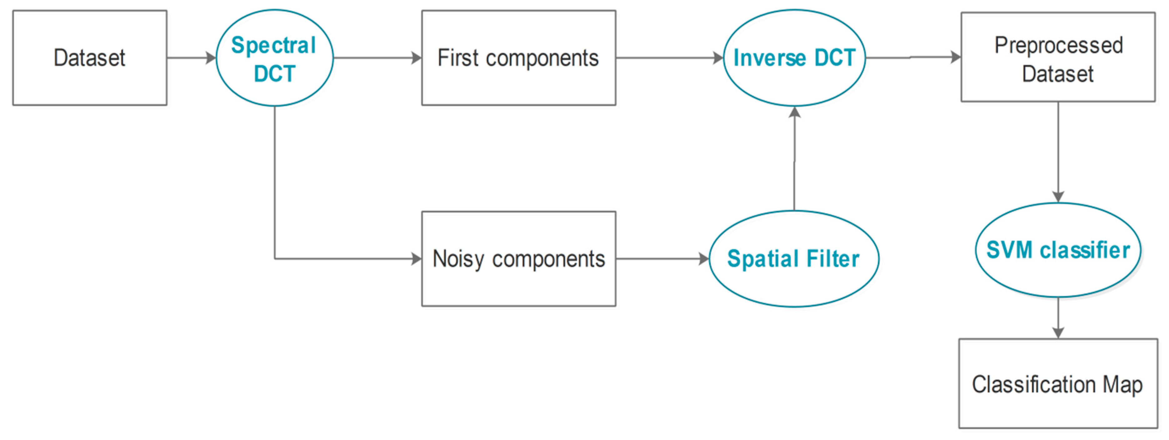
Figure 1. General flowchart of the spatial filtering in DCT domain-based classification framework for hyperspectral imagery.
Remotesensing 11 01405 g001
Figure 2. Detailed flowchart of the proposed spatial filtering in DCT domain-based frameworks for hyperspectral imagery classification.
Remotesensing 11 01405 g002
Figure 3. Flowchart of global 2D-DCT filtering step.
Remotesensing 11 01405 g003
Figure 4. The ground truth related information of Indian Pines image: (a) false-color composite, (b) ground truth map, (c) training map, (d) test map.
Remotesensing 11 01405 g004
Figure 5. The ground truth related information of Salinas image: (a) false-color composite, (b) ground truth map, (c) training map, (d) test map.
Remotesensing 11 01405 g005
Figure 6. The ground truth related information of Pavia University image: (a) false-color composite, (b) ground truth map, (c) training map, (d) test map.
Remotesensing 11 01405 g006
Figure 7. Overall Accuracy (OA%) with respect to the number of the first retained DCT coefficients in CDCT-2DCT_SVM on the Indian Pines, Salinas, and Pavia University datasets.
Remotesensing 11 01405 g007
Figure 8. Overall Accuracy (OA%) with respect to the different selected 2D-DCT thresholds in CDCT-2DCT_SVM on Indian Pines, Salinas, and Pavia University datasets.
Remotesensing 11 01405 g008
Figure 9. Overall Accuracy (OA%) with respect to the number of the first retained DCT coefficients in CDCT-WF_SVM on Indian Pines, Salinas, and Pavia University datasets.
Remotesensing 11 01405 g009
Figure 10. Overall Accuracy (OA%)with respect to the Wiener filter patch size in CDCT-WF_SVM on Indian Pines, Salinas, and Pavia University datasets.
Remotesensing 11 01405 g010
Figure 11. Classification maps created from the results of different methods on the Indian Pines dataset.
Remotesensing 11 01405 g011
Figure 12. Overall Accuracy (OA%) of the compared methods with different training samples proportions on Indian Pine dataset.
Remotesensing 11 01405 g012
Figure 13. Classification maps created from the results of different methods on the Salinas dataset.
Remotesensing 11 01405 g013
Figure 14. Overall Accuracy (OA%) of all methods with different training samples proportions on Salinas dataset.
Remotesensing 11 01405 g014
Figure 15. Classification maps created from the results of different methods on thePavia University dataset.
Remotesensing 11 01405 g015
Figure 16. Overall Accuracy (OA%) of all methods with different training samples proportions on the Pavia University dataset.
Remotesensing 11 01405 g016
Figure 17. Overall Accuracy (%) of all competing methods on clean and noisy Indian Pines dataset.
Remotesensing 11 01405 g017
Table 1. Classes of the Indian Pines scene with the number of testing and training samples.
ClassTypeSamplesTrainingTesting
1Alfalfa462323
2Corn-notill14281001328
3Corn-mintill830100730
4Corn237100137
5Grass-pasture483100383
6Grass-trees730100630
7Grass-pasture-mowed281414
8Hay-windrowed478100378
9Oats201010
10Soybean-notill972100872
11Soybean-mintill24551002355
12Soybean-clean593100493
13Wheat205100105
14Woods12651001165
15Buildings-Grass-Trees-Drives386100286
16Stone-Steel-Towers934746
Total 10,24912948955
Table 2. Classes of the Salinas scene with the related number of test and training samples.
ClassTypeSamplesTrainingTesting
1Brocoli greenweeds120091001909
2Brocoligreenweeds237261003626
3Fallow19761001876
4Fallowroughplow13941001294
5Fallowsmooth26781002578
6Stubble39591003859
7Celery35791003479
8Grapesuntrained11,27110011,171
9Soilvinyarddevelop62031006103
10Cornsenescedgreenweeds32781003178
11Lettuceromaine4wk1068100968
12Lettuceromaine5wk19271001827
13Lettuceromaine6wk916100816
14Lettuceromaine7wk1070100970
15Vinyarduntrained72681007168
16Vinyardverticaltrellis18071001707
Total 54,129160052,529
Table 3. Classes of the Pavia University scene with the related number of testing and training samples.
ClassTypeSamplesTrainingTesting
1Asphalt66313006331
2Meadows18,64930018,349
3Gravel20993001799
4Trees30643002764
5Painted metal sheets13453001045
6Bare Soil50293004729
7Bitumen13303001030
8Self-Blocking Bricks36823003382
9Shadows947300647
Total 42,776270040,076
Table 4. Summary of the compared methods with their abbreviations.
AbbreviationsMethods
SVM Support Vector Machine
PCA_SVMPrincipal Component Analysis followed by SVM
DCT_SVMSpectral one-dimensional Discrete Cosine Transform followed by SVM
2DCT_SVMTwo- dimensional DCT followed by SVM
CDCT-2DCT_SVMCascade spectral DCT spatial 2D-DCT followed by SVM
CDCT-WF_SVMCascade spectral DCT spatial Wiener filter followed by SVM
SDCT-2DCT_SVMSerial spectral DCT spatial 2D-DCT followed by SVM
S2DCT-DCT_SVMSerial spatial 2D-DCT spectral DCT followed by SVM
3D_SVMThree-dimensional Wavelet followed by SVM
3DG_ SVMThree-dimensional Wavelet with Graph Cut followed by SVM
EPFEdge-Preserving Filtering
IFRFImage Fusion and Recursive Filtering
BM4D_SVMBlock-Matching 4-D Filtering followed by SVM
PARAFAC_SVMParallel Factor Analysis followed by SVM
Table 5. Summary of the important parameters on different datasets.
MethodsParametersIndian PinesSalinasPavia University
CDCT-2DCT_SVM- The count of the retained Spectral DCT coefficients 101010
- 2D-DCT threshold500500500
CDCT-WF_SVM- The count of the retained Spectral DCT coefficients 555
- Wiener filter patch size39 × 3943 × 4331 × 31
PCA_SVMThe count of PCs 182045
All methodsThe training samples size per class100100300
Table 6. Classification results (%)on the Indian Pines dataset with standard deviation (in bracket).
ClassSVMPCA_SVMDCT_SVM2DCT_SVMSDCT-2DCT_SVMS2DCT-DCT_SVM3D_SVM3DG_SVMEPFIFRFBM4D_SVMPARAFAC_SVMCDCT-WF_SVMCDCT-2DCT_SVM
188.7078.2686.9690.0094.3584.7898.6898.70100.0071.7091.7493.4898.7096.96
272.7156.4471.5063.8377.5157.5876.4281.3185.7174.2583.2577.6492.1290.16
370.1159.4066.5568.1681.9054.7781.5990.9290.7949.7480.7873.9094.4495.00
480.9575.2686.5790.8097.1580.0098.3299.6465.0763.1591.6896.5097.8898.83
592.6988.9886.7492.6688.1281.6796.8997.1096.0180.5195.4892.8798.0997.42
695.2291.7087.5495.2593.4084.4497.2299.5699.4689.6096.6097.0899.2999.24
792.1478.5789.2997.8695.0088.5795.0097.14100.000.0087.8687.8696.4392.14
896.7595.7996.3598.8498.5795.08100.00100.00100.00100.0098.9999.68100.0099.79
978.0066.0080.0084.0089.0072.00100.0097.00100.000.0089.0094.00100.0099.00
1072.9955.0968.1460.5671.3648.8680.9189.9171.3461.4882.2678.4190.9290.01
1156.2446.8248.9146.3753.9334.0075.2383.7291.6994.1968.7470.2890.6482.70
1272.7251.8970.6559.4777.8744.9991.0396.4166.3942.1183.8780.3494.0295.72
1398.7696.8697.0599.5299.0597.3399.1499.71100.0081.7699.1499.3399.7199.43
1485.9586.4783.5890.6488.8878.6495.7296.2199.2497.8992.4691.7998.8999.30
1571.4760.2468.3286.7192.9071.5795.1099.9378.4779.0988.4392.6998.1598.60
1697.3997.6197.17100.0099.7899.5798.9192.8393.6797.5096.7499.3596.9698.48
κ70.40
(0.79)
59.63
(1.24)
65.83
(1.32)
65.27
(0.74)
73.07
(0.87)
53.34
(1.62)
83.84
(0.78)
88.87
(1.18)
84.68
(1.96)
71.06
(1.66)
80.66
(0.64)
78.95
(1.03)
93.44
(1.03)
90.81
(1.05)
OA73.97
(0.71)
64.40
(1.13)
69.82
(1.19)
69.33
(0.71)
76.27
(0.80)
58.46
(1.63)
86.12
(0.70)
90.32
(1.04)
85.61
(1.72)
74.30
(1.46)
83.08
(0.56)
81.62
(0.92)
94.31
(1.05)
92.01
(0.92)
AA82.67
(0.97)
74.09
(1.41)
80.33
(1.59)
82.79
(0.89)
87.42
(1.13)
73.37
(1.36)
92.51
(0.72)
95.01
(0.70)
89.87
(1.60)
67.69
(1.80)
89.19
(0.87)
89.08
(1.00)
96.64
(0.56)
95.80
(0.43)
Time(s)3.1042.7243.374.1215.9553.2453.41210.166.801.48351.37297.3913.3013.91
The bold values indicate critical values.
Table 7. Classification results (%) on the Salinas dataset with standard deviation (in brackets).
ClassSVMPCA_SVMDCT_SVM2DCT_SVMSDCT-2DCT_SVMS2DCT-DCT_SVM3D_SVM3DG_SVMEPFIFRFBM4D_SVMPARAFAC_SVMCDCT-WF_SVMCDCT-2DCT_SVM
199.1399.3697.5399.6497.0296.8999.1999.70100.0098.9999.2597.3399.5299.50
299.5199.5298.8399.1396.6497.4399.3599.6899.97100.0099.6396.0599.7899.59
399.5899.0999.4794.8891.9290.3697.4898.9596.0799.8499.7796.0898.9799.39
499.3499.3599.1898.9898.5697.9899.3699.4398.4390.0599.3096.0299.2399.51
598.7497.7898.0396.5794.8494.1798.9899.4699.8099.9898.5586.1498.3698.25
699.6899.6799.6899.7199.7499.7499.8699.9599.99100.0099.6799.4499.6299.65
799.5799.5699.4599.6599.0297.3199.6699.6799.9399.7999.5598.5899.6599.64
867.9872.4074.4070.8763.4959.7586.2788.6785.4099.5378.0077.1394.8591.46
999.0097.5098.0998.6096.4796.8698.4399.1898.7399.9899.4788.5299.4699.41
1095.0194.5193.1793.5490.1989.7493.7995.6093.6099.7296.3673.2897.7695.15
1198.9098.7597.2397.2294.2994.6399.6899.9397.5899.0298.9785.2398.8099.52
1299.8299.7099.5797.6295.6489.5999.9799.8799.6798.8299.8482.1999.9399.93
1399.5899.5598.1399.1798.0395.6999.0298.9799.8397.7099.7289.3499.4699.90
1497.7697.9295.5997.7098.4396.5598.0198.1997.8997.5898.4393.8998.1299.04
1570.0470.5169.7170.5565.8464.2275.9285.5277.6883.0679.7281.5696.1993.62
1698.8698.8898.5198.7197.8796.0798.8398.7099.71100.0098.4895.7298.8799.21
κ87.04
(0.62)
87.86
(1.07)
87.96
(0.86)
87.20
(0.73)
83.52
(0.53)
81.86
(0.95)
92.05
(0.41)
94.44
(0.89)
92.13
(0.90)
96.28
(0.27)
91.04
(0.69)
85.49
(0.47)
97.62
(0.33)
96.30
(0.80)
OA88.36
(0.57)
89.10
(0.97)
89.20
(0.78)
88.51
(0.65)
85.18
(0.48)
83.69
(0.86)
92.88
(0.37)
95.02
(0.79)
92.95
(0.81)
96.46
(0.25)
91.96
(0.62)
86.94
(0.73)
97.86
(0.30)
96.68
(0.72)
AA95.16
(0.20)
95.25
(0.41)
94.78
(0.34)
94.53
(0.36)
92.37
(0.23)
91.06
(0.45)
96.49
(0.15)
97.59
(0.36)
96.52
(0.31)
97.65
(0.29)
96.54
(0.21)
89.78
(0.39)
98.66
(0.16)
98.30
(0.32)
Time(s)7.2413.1864.4612.8190.42102.00183.591142.5219.294.771854.071634.361.2270.56
The bold values indicate critical values.
Table 8. Results (%) on the Pavia University dataset with standard deviation (in brackets).
ClassSVMPCA_SVMDCT_SVM2DCT_SVMSDCT-2DCT_SVMS2DCT-DCT_SVM3D_SVM3DG_SVMEPFIFRFBM4D_SVMPARAFAC_SVMCDCT-WF_SVMCDCT-2DCT_SVM
171.7172.1374.5958.6754.5465.5296.8998.8898.6876.1880.0777.9097.9696.21
282.9182.7979.1665.9060.7567.1497.6498.9197.2097.9089.4985.3799.6698.02
378.8978.2381.8961.8654.5762.0188.1590.0892.5152.3982.6170.8198.8797.23
491.8991.0086.2887.6483.4980.3499.0199.4267.8184.9994.1593.8595.9297.38
599.7099.7099.7599.8999.9299.88100.00100.0099.8998.8599.6699.7899.7899.77
684.3977.9468.4563.6356.1355.2496.6899.1664.3192.7489.7684.8399.3998.16
776.9677.5784.9860.9657.3671.2798.9199.5377.2564.2285.5977.8999.4998.63
869.4471.0775.5453.5947.3559.5694.6496.0884.4053.2475.8874.3097.6293.75
999.9199.8699.9499.7299.7799.8699.6399.7296.1743.6399.8899.9299.8899.91
κ75.24
(1.43)
74.25
(2.16)
71.74
(1.15)
56.52
(1.95)
50.32
(1.39)
57.58
(1.36)
95.88
(0.30)
97.82
(0.12)
82.79
(1.03)
77.63
(0.25)
83.00
(1.40)
80.91
(0.47)
97.87
(0.26)
96.48
(0.42)
OA81.18
(1.15)
80.49
(1.75)
78.51
(1.14)
66.07
(1.56)
60.95
(2.00)
67.01
(1.82)
96.95
(0.22)
98.39
(0.09)
86.81
(1.68)
83.14
(0.19)
87.23
(1.10)
83.99
(0.40)
98.71
(0.19)
97.40
(0.32)
AA83.98
(0.69)
83.37
(1.68)
83.40
(1.73)
72.43
(1.47)
68.21
(1.64)
73.42
(1.52)
96.84
(0.14)
97.98
(0.12)
86.47
(1.01)
73.79
(0.17)
88.57
(0.79)
84.96
(0.40)
98.73
(0.19)
97.67
(0.18)
Time(s)80.0578.68186.10116.79252.69216.92485.922142.4052.8418.141535.131275.06124.93142.74
The bold values indicate critical values.