A Fisheye Image Matching Method Boosted by Recursive Search Space for Close Range Photogrammetry

Abstract

Close range photogrammetry (CRP) with large field-of-view images has become widespread in recent years, especially in terrestrial mobile mapping systems (TMMS). However, feature-based matching (FBM) with omnidirectional images (e.g., fisheye) is challenging even for state-of-the-art methods, such as the scale-invariant feature transform (SIFT), because of the strong scale change from image to image. This paper proposes an approach to boost FBM techniques on fisheye images with recursive reduction of the search space based on epipolar geometry. The epipolar restriction is calculated with the equidistant mathematical model and the initial exterior orientation parameters (EOPs) determined with navigation sensors from TMMS. The proposed method was assessed with data sets acquired by a low-cost TMMS. The TMMS is composed of a calibrated poly-dioptric system (Ricoh Theta S) and navigation sensors aimed at outdoor applications. The assessments show that Ricoh Theta S position and attitude were estimated in a global bundle adjustment with a precision (standard deviation) of 4 cm and 0.3°, respectively, using as observations the detected matches from the proposed method. Compared with other methods based on SIFT extended to the omnidirectional geometry, our approach achieved compatible results for outdoor applications.

1. Introduction

Omnidirectional systems enable a 360° coverage around the sensor, tracking more features in a single image, which encourages the use of these sensors in structure from motion (SfM) approaches. Furthermore, lightweight and low-cost omnidirectional cameras have recently entered in the market with significant improvements in terms of device developments and data processing. An accurate solution using SfM depends on a strong network configuration of tie points. The network configuration requires high accurate image measurements, suitable geometric distribution in the images, and an optimal number of tie points. Therefore, the main challenge of SfM using omnidirectional images for close range photogrammetry (CRP) applications relies on the automatic detection of image observations. The applicability of omnidirectional sensors requires adaptations to the classic photogrammetric process, such as image matching, due to the specific sensor geometry. Several challenges remain in the treatment of images acquired by sensors with non-perspective inner geometry, such as large scale and illumination variations between scenes, large radial distortion, and nonuniformity of spatial resolution. Therefore, many studies have focused on extending the well-known feature-based matching (FBM) algorithms from perspective to omnidirectional images, aiming SfM solutions.

Three trends in omnidirectional image-matching issues can be noted [1]. The first possibility (approach A) is conversion of a wide-angle image into a geometrically corrected perspective image [2,3,4], and thus standard FBM algorithms can be considered geometrically valid. However, this reprojection can add radiometric and geometric distortions and image information losses. Alternatively, the original wide-angle images can be used with consideration of performed consistent geometric modifications in the image-matching approach, such as in feature extraction or feature comparison. Therefore, a second option (approach B) adapts existing interest operators, such as SIFT (scale-invariant feature transform) [5], using a spherical surface as a nondeformable domain for image operations [6]. This approach requires an adaptive scale-space function defined on the sphere. Various research studies were developed in this direction, with the aim of efficiently solving the problem of feature detection of the sphere surface without introducing image artifacts [1,7,8,9,10,11]. It is well known that FBM techniques are limited by the quality of the interest point and the features extracted. The works mentioned in References [6,7,8,9,10,11] proposed geometrically rigorous methods for interest point detection in omnidirectional images, which are of wide interest for 3D reconstruction. However, complex implementation and high computation efforts are required. Generally, the number of correct matches tracked by standard FBM algorithms on an omnidirectional image is beyond the minimum number of points required for robust sensor orientation estimation based on SfM. A third possibility (approach C) focuses on improving the features comparison of SIFT descriptors to reduce mismatches, mainly in outdoor mapping, for which additional information such as camera positions determined with a GNSS (global navigation satellite system) is commonly available.

Currently, imaging and navigation systems are combined in mobile mapping platforms, enabling an integrated SfM solution. Therefore, considering that the imaging system model is known and that the initial camera position and attitude are supplied by the navigation systems, the position of the searched feature can be predicted, and outliers reduced [12,13,14,15,16,17,18,19]. Scaramuzza et al. [12] used a calibrated omnidirectional camera arranged in a vehicle roof for outdoor mobile mapping. The SIFT operator was combined with a filter based on random sample consensus (RANSAC) to remove outliers, and to retain the reliable homologous points for sensor position estimation. In this approach, outliers were successfully removed by RANSAC, however, features distribution throughout the omnidirectional keyframes in the data set was still a problem. Valgren and Lilienthal [13] evaluated the performance of two interest operators (SIFT and speeded-up robust features (SURF)) for outdoor panoramic images acquired in different seasons with a mobile mapping system composed of an omnidirectional camera and a GNSS receiver embedded in a robotic platform. Improvements in the SIFT and SURF performances were obtained by changing the matching metric and the acceptance threshold for descriptor comparison according to the data sets evaluated. Additionally, the operators were tested in different panoramic image resolutions and with the use of epipolar constraints to eliminate false matches. The computational time and match correctness benefits of reducing the search space, e.g., based on epipolar geometry, are well known for perspective images. Therefore, certain authors extended the classical mathematical model of the perspective epipolar concept [14] to omnidirectional sensor geometry [15,16,17]. More recently, Valiente et al. [18] proposed a similar strategy to improve image matching with an adaptation of the epipolar constraint for an omnidirectional system composed of a calibrated omnidirectional camera, internal odometer, and a laser range finder mounted on a four-wheel robotic platform. A search window was defined based on the epipolar line position, propagation of the current omnidirectional system uncertainty, and extended Kalman filter (EKF) prediction.

Previous approaches [12,13,18,19] have inspired the method for fisheye image matching proposed in this paper (approach C). To this end, we propose a technique that reduces the search space window recursively in the fisheye images based on the epipolar geometry constraint in the sphere domain and applies the equidistant mathematical model. Experiments and assessments were performed that combine the search space technique with the interest operator SIFT [5], which is one of the most popular interest operators, particularly due to robust matching even in affine distortion cases. Data sets were collected using a low-cost mobile mapping system [20] composed of a calibrated poly-dioptric camera (Ricoh Theta S) and a GNSS/IMU (inertial measurement unit) navigation system. In summary, the main contributions of our paper are: (1) a simplified technique for epipolar constraint in the sphere domain considering the equidistant projection model, (2) a recursive approach to reducing the search window, and (3) analysis of outdoor CRP applications and real data collected with an assembled lightweight system in forest and urban areas.

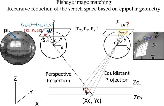
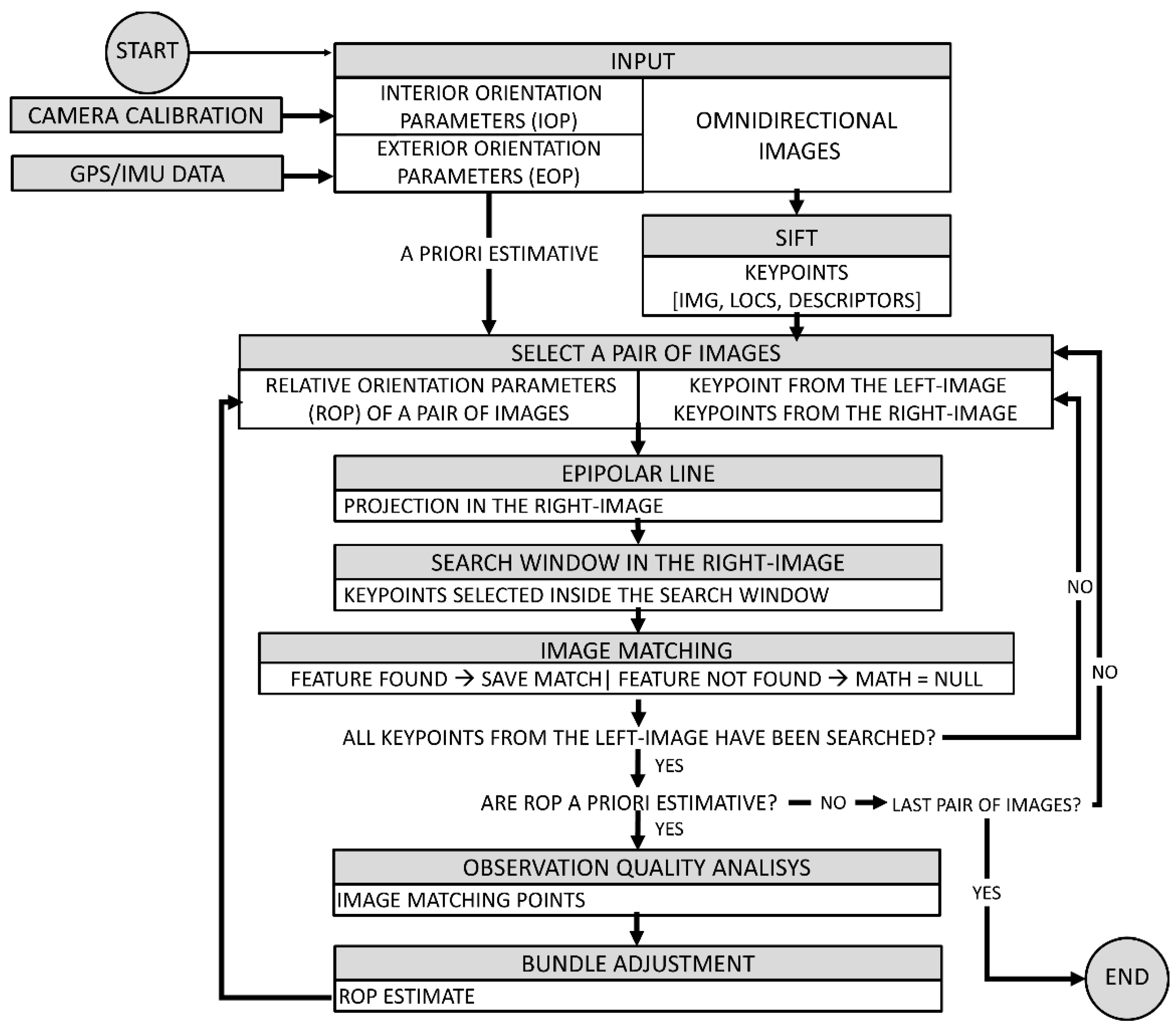
2. Recursive Search Space Method for Fisheye Images

Figure 1 presents a flow chart of the proposed method for recursive feature search (RFS) in fisheye images. The input data include the interior orientation parameters (IOPs) from a previous camera calibration process [21], the initial exterior orientation parameters (EOPs) acquired by a navigation system (global positioning system (GPS) receiver and IMU), and omnidirectional images. The relative orientation parameters (ROP) encompassing the base elements (B_X, B_Y, and B_Z) and relative rotations (Δω, Δϕ, and Δκ) between consecutive images were estimated based on the initial EOPs.

Considering a minimum of two fisheye images, the SIFT technique was applied to detect interest points (key points) in all images covering the scene. Section 4.1 discusses the motivation of SIFT choice. An iterative process is performed from each possible pair of images (left and right images). For each key point extracted in the first image (left image) a search window is defined in the right image based on the epipolar line projection (see Section 2.1), and the invariant descriptor vector from the key point searched is compared only with the key points belonging to that search window. The search window is computed as a function of the IOPs and ROPs, and its dimensions depend on the initial EOP uncertainty. Subsequently, recursive bundle adjustment is performed to improve the ROP estimated, thus reducing the search window dimensions (see Section 2.2). The homologue points used in the first iteration are evaluated and selected, using the minimum standardized Euclidean distance and the maximum correlation coefficient between key point features (see Section 2.3) as quality metrics. The assumptions made in the following sections refer to a pair of images, but they can be generalized to successive pairs in a sequence of images.

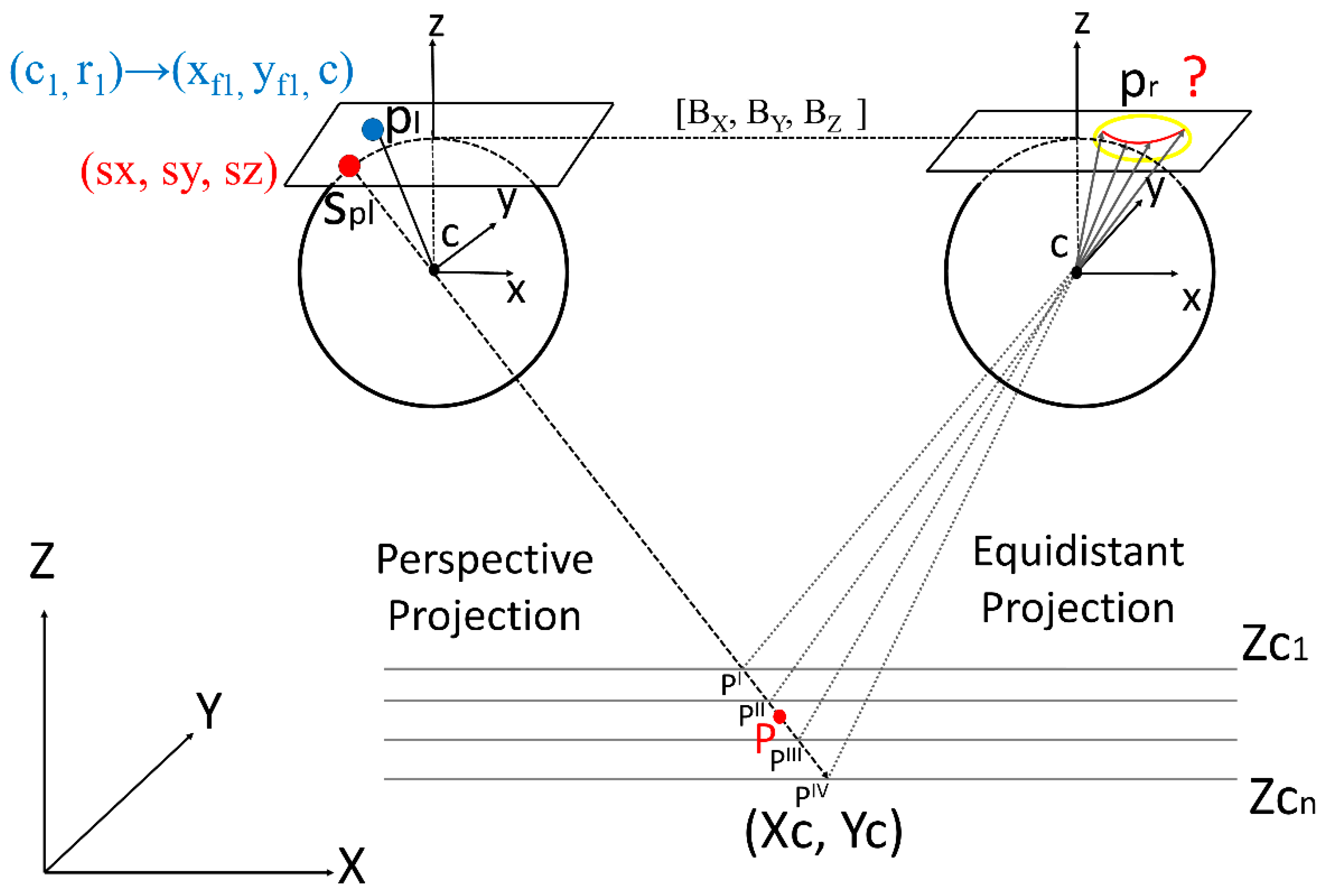
2.1. Epipolar Geometry on the Sphere Domain

Considering a pair of images, the image location of a key point from the left image can be predicted in the right image using a geometric search approach, such as those based on epipolar geometry. The principle of epipolar geometry consists of coplanarity between a point P with coordinates X, Y, and Z in the object space and the perspective centers (PCs) of the cameras forming the image pair with coordinates X_PCL, Y_PCL, and Z_PCL and X_PCR, Y_PCR, and Z_PCR that cover point P. Considering perspective geometry, the intersection between the epipolar plane formed by point P and the PCs and the image planes results in two lines, known as conjugated epipolar lines. The projections of point P in the left (p_l) and right image (p_r) are constrained to fit on the conjugated epipolar lines in the respective images. The epipolar line can be estimated with different methods based on the relative orientation between images [22,23], such as the solution with eight or more point matches, an analytic method with a rank-2 constraint, a gradient-based technique, and the least median of squares (LMedS). In summary, consecutive estimation of the ROP is an iterative process that requires a set of homologous points (n ≥ 7) and an estimation technique.

Certain modifications in the classical approaches must be considered for estimation of the epipolar line shape and position in the fisheye images. For instance, considering the omnidirectional image geometry, the epipolar lines are curves [17]. We propose a simplified approach based on projection of an interest point in the left image to the object space using the inverse collinearity condition on the sphere domain, and subsequently, the reprojection to the right image using the equidistant equations. The epipolar line position is recursively refined with the improvements in the relative orientation estimation (Section 2.2). Figure 2 summarizes the proposed method.

If the IOPs and ROPs between consecutive images are known, the position of the epipolar lines can be estimated. The IOPs were previously determined in a camera calibration process [21]. As mentioned, the ROP base elements (B_X, B_Y, and B_Z) and attitude changes (Δω, Δϕ, and Δκ) between consecutive images were estimated based on the initial EOPs measured by a navigation system (GNSS/IMU). The left image is considered as the origin of the local system, and therefore, the PC coordinates (X_PCL, Y_PCL, and Z_PCL) and the rotations (ω_L, ϕ_L, and κ_L) can be assumed equal to zero or to the nominal values acquired by the navigation system. With the former option, the PC coordinates of the right image (X_PCR, Y_PCR, and Z_PCR) are the base elements (B_X, B_Y, and B_Z), and the rotations (ω_R, ϕ_R, and κ_R) are the relative angles (Δω, Δϕ, and Δκ) between consecutive images.

Because the parameters are known, it is possible to project an interest point p_l from the left image to the object space (P) and subsequently re-project to the right image (p_r). The projection from p_l in the image space to the object space can be accomplished by projecting from the sensor plane to the sphere and also to the object space using the inverse collinearity equation. Since fisheye images do not follow perspective geometry, the collinearity equation is not geometrically valid for the original fisheye coordinates in the image plane. However, the collinearity equation can be considered valid after a projection of the image coordinates from the image plane to a sphere, which is a spatial domain free from deformation. Therefore, the row and column coordinates measured in the left image (c₁, r₁) are computed in the photogrammetric image system (x_f1, y_f1), as presented in Equation (1):

$$\begin{gathered} {\mathrm{x}}_{\mathrm{f}1}=\left[\mathrm{s}*\left({\mathrm{c}}_1-{\mathrm{c}}_{\mathrm{x}}\right)\right]-{\mathrm{x}}_0+{\Delta }_{\mathrm{x}},\mathrm{and} \\ {\mathrm{y}}_{\mathrm{f}1}=\left[-\mathrm{s}*\left({\mathrm{r}}_1-{\mathrm{c}}_{\mathrm{y}}\right)\right]-{\mathrm{y}}_0+{\Delta }_{\mathrm{y}}, \end{gathered}$$

(1)

where (s) is the pixel size in mm, (x₀, y₀) are the principal point coordinates, (c_x, c_y) are the coordinates of the geometric image center, and (Δ_x, Δ_y) are the corrections of lens distortions. Thus, p_l (x_f1, y_f1) is projected to a sphere (s_x, s_y, s_z) with a radius equal to the principal distance (c) using Equation (2), which considers the equidistant property [24].

$${\mathrm{s}}_{\mathrm{x}}=\mathrm{c}*\cos \mathsf{\theta }*\sin \mathsf{\alpha };{\mathrm{s}}_{\mathrm{y}}=\mathrm{c}*\sin \mathsf{\theta }*\sin \mathsf{\alpha };{\mathrm{s}}_{\mathrm{z}}=\mathrm{c}*\cos \mathsf{\alpha },$$

(2)

where α is the incident angle, and θ is the angle formed by the radius (r_d) of an image point and the x-axis in the image (Equation (3)).

$${\mathrm{r}}_{\mathrm{d}}=\sqrt{{\mathrm{x}}_{\mathrm{f}1}{}^2+{\mathrm{y}}_{\mathrm{f}1}{}^2};\mathsf{\alpha }=\left(\frac{{\mathrm{r}}_{\mathrm{d}}}{\mathrm{c}}\right)\mathrm{rad};\mathsf{\theta }={\tan }^{-1}\left(\frac{{\mathrm{y}}_{\mathrm{f}1}}{{\mathrm{x}}_{\mathrm{f}1}}\right).$$

(3)

The coordinates of p_l on the sphere (s_x, s_y, s_z) can be projected to the object space P (X, Y, Z) using the collinearity principle in a mono-restitution process. Because the depth of point P is also unknown, a set of planes is considered. The number of planes used (i) and the ranging of Z values needs to be previously determined based on existing knowledge about the scene and the dataset used. Therefore, for each Z(i) supplied, the X(i) and Y(i) coordinates are estimated as presented in Equation (4) in which λ(i) are scale factors (Equation (5)), and m_ij (i and j from 1 to 3) are rotation matrix elements related to the left-image attitude (origin of the local system), resulting in an identity matrix.

$$\begin{gathered} {\mathrm{X}}_{\left(\mathrm{i}\right)}={\mathrm{X}}_{\mathrm{CPL}}+{\mathsf{\lambda }}_{\left(\mathrm{i}\right)}*\left[{\mathrm{m}}_{11}·{\mathrm{s}}_{\mathrm{x}}+{\mathrm{m}}_{21}·{\mathrm{s}}_{\mathrm{y}}+{\mathrm{m}}_{31}·{\mathrm{s}}_{\mathrm{z}}\right],\mathrm{and} \\ {\mathrm{Y}}_{\left(\mathrm{i}\right)}={\mathrm{Y}}_{\mathrm{CPL}}+{\mathsf{\lambda }}_{\left(\mathrm{i}\right)}*\left[{\mathrm{m}}_{12}·{\mathrm{s}}_{\mathrm{x}}+{\mathrm{m}}_{22}·{\mathrm{s}}_{\mathrm{y}}+{\mathrm{m}}_{32}·{\mathrm{s}}_{\mathrm{z}}\right]. \end{gathered}$$

(4)

$${\mathsf{\lambda }}_{\left(\mathrm{i}\right)}=({\mathrm{Z}}_{\left(\mathrm{i}\right)}-{\mathrm{Z}}_{\mathrm{CPL}})/\left[{\mathrm{m}}_{13}·{\mathrm{s}}_{\mathrm{x}}+{\mathrm{m}}_{23}·{\mathrm{s}}_{\mathrm{y}}+{\mathrm{m}}_{33}·{\mathrm{s}}_{\mathrm{z}}\right].$$

(5)

Finally, the computed X(i) and Y(i) coordinates are projected to the right image (x_f2, y_f2) using the ROPs as EOPs for the right image and the equidistant equations [24,25] because this is the fisheye model on which the Ricoh Theta S lenses are based (Equation (6)). Another fisheye mathematical model can also be used to model the lens geometry [24,25]. Distortion corrections are added to these coordinates in the photogrammetric image system and converted to the column-row system (c₂, r₂). Equation (6) shows the equidistant mathematical model to estimate the right image coordinates (x_f2, y_f2), in which X_c, Y_c, and Z_c are computed in function of the base elements (B_X, B_Y, and B_Z) and the relative orientation matrix m_R (Δω, Δϕ, and Δκ), as presented in Equation (7).

$${\mathrm{x}}_{\mathrm{f}2}=-\mathrm{c}·\frac{{\mathrm{X}}_{\mathrm{c}}}{\sqrt[2]{{\mathrm{X}}_{\mathrm{c}}{}^2+{\mathrm{Y}}_{\mathrm{c}}{}^2}}·\arctan \left(\frac{\sqrt[2]{{\mathrm{X}}_{\mathrm{c}}{}^2+{\mathrm{Y}}_{\mathrm{c}}{}^2}}{{\mathrm{Z}}_{\mathrm{c}}}\right);{\mathrm{y}}_{\mathrm{f}2}=-\mathrm{c}·\frac{{\mathrm{Y}}_{\mathrm{c}}}{\sqrt[2]{{\mathrm{X}}_{\mathrm{c}}{}^2+{\mathrm{Y}}_{\mathrm{c}}{}^2}}·\arctan \left(\frac{\sqrt[2]{{\mathrm{X}}_{\mathrm{c}}{}^2+{\mathrm{Y}}_{\mathrm{c}}{}^2}}{{\mathrm{Z}}_{\mathrm{c}}}\right),$$

(6)

where

$$\begin{gathered} {\mathrm{X}}_{\mathrm{C}\left(\mathrm{i}\right)}={\mathrm{m}}_{\mathrm{R}11}*\left({\mathrm{X}}_{\left(\mathrm{i}\right)}-{\mathrm{B}}_{\mathrm{X}}\right)+{\mathrm{m}}_{\mathrm{R}12}*\left({\mathrm{Y}}_{\left(\mathrm{i}\right)}-{\mathrm{B}}_{\mathrm{Y}}\right)+{\mathrm{m}}_{\mathrm{R}13}*\left({\mathrm{Z}}_{\left(\mathrm{i}\right)}-{\mathrm{B}}_{\mathrm{Z}}\right), \\ {\mathrm{Y}}_{\mathrm{C}\left(\mathrm{i}\right)}={\mathrm{m}}_{\mathrm{R}21}*\left({\mathrm{X}}_{\left(\mathrm{i}\right)}-{\mathrm{B}}_{\mathrm{X}}\right)+{\mathrm{m}}_{\mathrm{R}22}*\left({\mathrm{Y}}_{\left(\mathrm{i}\right)}-{\mathrm{B}}_{\mathrm{Y}}\right)+{\mathrm{m}}_{\mathrm{R}23}*\left({\mathrm{Z}}_{\left(\mathrm{i}\right)}-{\mathrm{B}}_{\mathrm{Z}}\right), \\ {\mathrm{Z}}_{\mathrm{C}\left(\mathrm{i}\right)}={\mathrm{m}}_{\mathrm{R}31}*\left({\mathrm{X}}_{\left(\mathrm{i}\right)}-{\mathrm{B}}_{\mathrm{X}}\right)+{\mathrm{m}}_{\mathrm{R}32}*\left({\mathrm{Y}}_{\left(\mathrm{i}\right)}-{\mathrm{B}}_{\mathrm{Y}}\right)+{\mathrm{m}}_{\mathrm{R}33}*\left({\mathrm{Z}}_{\left(\mathrm{i}\right)}-{\mathrm{B}}_{\mathrm{Z}}\right). \end{gathered}$$

(7)

2.2. Search Space Window and Bundle Adjustment

The initial relative orientation between images was estimated with the data from a navigation system. The navigation system is commonly composed of a GNSS receiver and an IMU. These sensor measurements are affected by error related to the equipment and its physical components, the synchronization of the components, and the method of data processing. In a first iteration of the proposed method, the accuracy of the epipolar line position was related to the ROP accuracy and consequently was affected by navigation system errors. Therefore, a window surrounding the line can be defined as a search space. For each point projected, an error ellipse was computed based on the error propagation of the ROP. A polygon (convex hull) was fitted surrounding these ellipses, thus determining the search space. Considering an interest point defined in the left image (Figure 3a), the corresponding point was searched only inside this search window (Figure 3b), thus reducing false matches and the computation time. Figure 3 illustrates this process in which (a) presents an interest point in the left image (green) and (b) shows the epipolar line (red), the error ellipses (blue), and the search window (yellow) defined in the right image.

The errors in the ROP initially estimated from navigation data can be minimized by the bundle adjustment based on the least squares method. The epipolar line position can be improved in an iterative process, and the search window dimensions can be updated based on the standard deviation of the estimated ROP. In this work, the bundle adjustment was implemented using the least square method according to Mikhail and Ackerman [26].

The equidistant equations were considered as the mathematical model in the bundle adjustment. The approximated parameter values and observations used as input data in the bundle adjustment were selected from the first image-matching iteration in which the search window dimensions were related to the navigation data error. For each pair of images, at least seven well distributed pairs of matches were automatically chosen as observations using the minimum standard Euclidean distance and maximum correlation between key point vector features as quality criteria, as discussed in Section 2.3. Furthermore, a statistical test (Pope test) was performed during the bundle adjustment to eventually reduce the weight of potential wrong observations (mismatches) based on the normalized standard deviation and the t-Student distribution of 95% sigma [27].

2.3. Image Matching

Homologue points are defined by comparing the SIFT features of a point (i ranging between 1 and n) in the left image H1_(i) with the SIFT features of the points (j to m) inside of the search space window in the right image (H2_(j,…,m), with j = 1 and m equal to the number of features inside of the search space window), as shown in Figure 3. The correct selection of homologous features requires an appropriate metric for key point comparison. Therefore, the similarity between SIFT features H1_(1,…,n) and H2_(j,…,m) can be computed with different metrics. The standard SIFT algorithm [5] considers the minimum Euclidean distance (D_E, Equation (8)a) as the similarity criterion. However, a different metric for image matching could improve the performance of image matching using SIFT [28]. Other criteria can also be used to select the nearest neighbor, such as standardized Euclidean distance (D_Eσ, Equation (8)b), chi-square distance (Dχ², Equation (8)c), Hellinger distance (D_HE, Equation (8)d), and histogram correlation (ρ, Equation (8)e). The five metrics [29] have been combined with SIFT implementation to assess which approach fits best for FBM with fisheye images from outdoor environments.

$$\begin{array}{cccc}{\mathrm{D}}_{\mathrm{E}}=\sqrt{{(\mathrm{H}{1}_{\left(\mathrm{i}\right)}-\mathrm{H}{2}_{\left(1,\dots ,\mathrm{m}\right)})}^2}\hfill & \hfill \left(\mathrm{a}\right)& {\mathrm{D}}_{\mathrm{E}\mathsf{\sigma }}=\sqrt{\frac{{(\mathrm{H}{1}_{\left(\mathrm{i}\right)}-\mathrm{H}{2}_{\left(1,\dots ,\mathrm{m}\right)})}^2}{\mathrm{s}}}\hfill & \hfill \left(\mathrm{b}\right)\\ {\mathrm{D}}_{{\mathsf{\chi }}^2}={\displaystyle \sum }_{\mathrm{i}}^{\mathrm{n}}\frac{{\left(\mathrm{H}{1}_{\left(\mathrm{i}\right)}-\mathrm{H}{2}_{\left(1,\dots ,\mathrm{m}\right)}\right)}^2}{\mathrm{H}{1}_{\left(\mathrm{i}\right)}+\mathrm{H}{2}_{\left(1,\dots ,\mathrm{m}\right)}}\hfill & \hfill \left(\mathrm{c}\right)& {\mathrm{D}}_{\mathrm{HE}}={(\mathrm{H}{1}_{\left(\mathrm{i}\right)}{}^5-\mathrm{H}{2}_{\left(1,\dots ,\mathrm{m}\right)}{}^5)}^2\hfill & \hfill \left(\mathrm{d}\right)\\ \mathsf{\rho }=1-\frac{(\mathrm{H}{1}_{\left(\mathrm{i}\right)}-\overline{\mathrm{H}1})(\mathrm{H}{2}_{\left(1,\dots ,\mathrm{m}\right)}-\overline{\mathrm{H}2})}{\sqrt{{(\mathrm{H}{1}_{\left(\mathrm{i}\right)}-\overline{\mathrm{H}1})}^2+{(\mathrm{H}{2}_{\left(1,\dots ,\mathrm{m}\right)}-\overline{\mathrm{H}2})}^2}}\hfill & \hfill \left(\mathrm{e}\right)& \hfill & \hfill \end{array}$$

(8)

Based on the computed distances, the nearest neighbor of a feature descriptor was selected and assessed to decide whether the second-closest neighbor distance is smaller than a threshold value. This criterion used to select or reject a match is more effective than a global threshold. Originally, a value of 0.8 was suggested as a threshold for the relationship between the nearest and second nearest neighbor key points [5]. However, this value must be defined according to the data set. In this regard, we performed a preliminary study focuses on fisheye images from outdoor environments using data set III (Figure 7c). This data set was collected with a mobile mapping system (Figure 6) in a test area with sparse vegetation and urban features (e.g., buildings). More details will be presented in Section 3.1 (data set III). To cope with the large variation in surroundings of a feature in fisheye images, thresholds of 0.5 for linear distances and (0.5)² for squared distances and correlations were applied in our experiments. These thresholds were defined based on a preliminary assessment that evaluated SIFT performance in the data set used. Figure 4 presents the total of matches (detection rate) and the correct points detected (location accuracy in percentage) for each metric approach (distances) used as matching criteria.

Three approaches can be highlighted in terms of performance compared with the classical Euclidean distance (70% of correct detection). The standardized Euclidean (76%), chi-square (76%), and Hellinger (74%) distances improved the number of corrected match detection along the fisheye image, as also noted in [28]. This result means that, on average, 10 matches in a pair of images (data set III, Section 3.1) were better selected using one of the metrics other than the Euclidean distance. Considering this result, the standardized Euclidean distance was used as a metric for feature comparison in the proposed method.

3. Material and Experiments

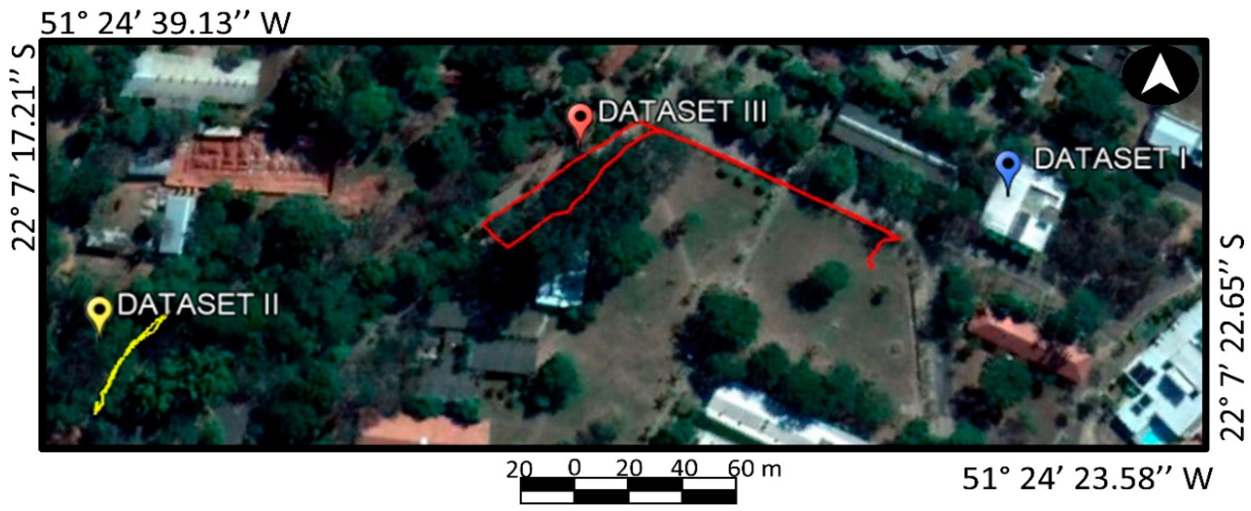
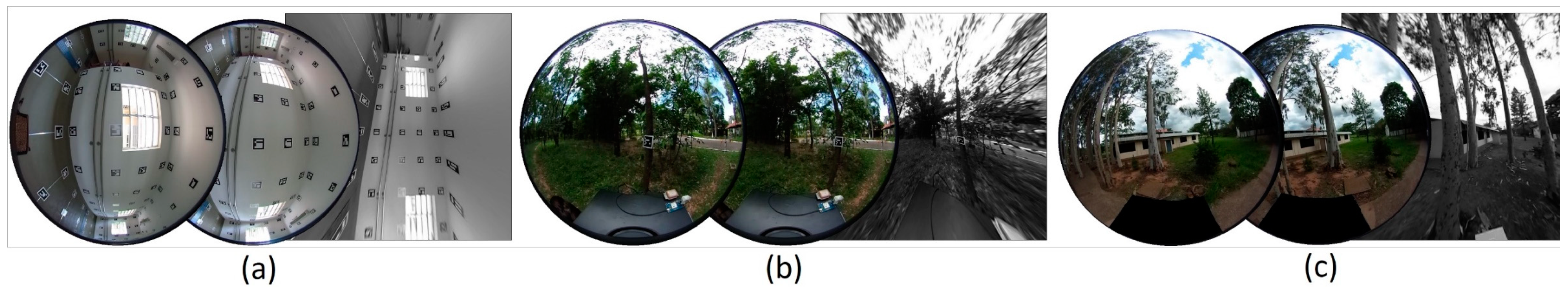
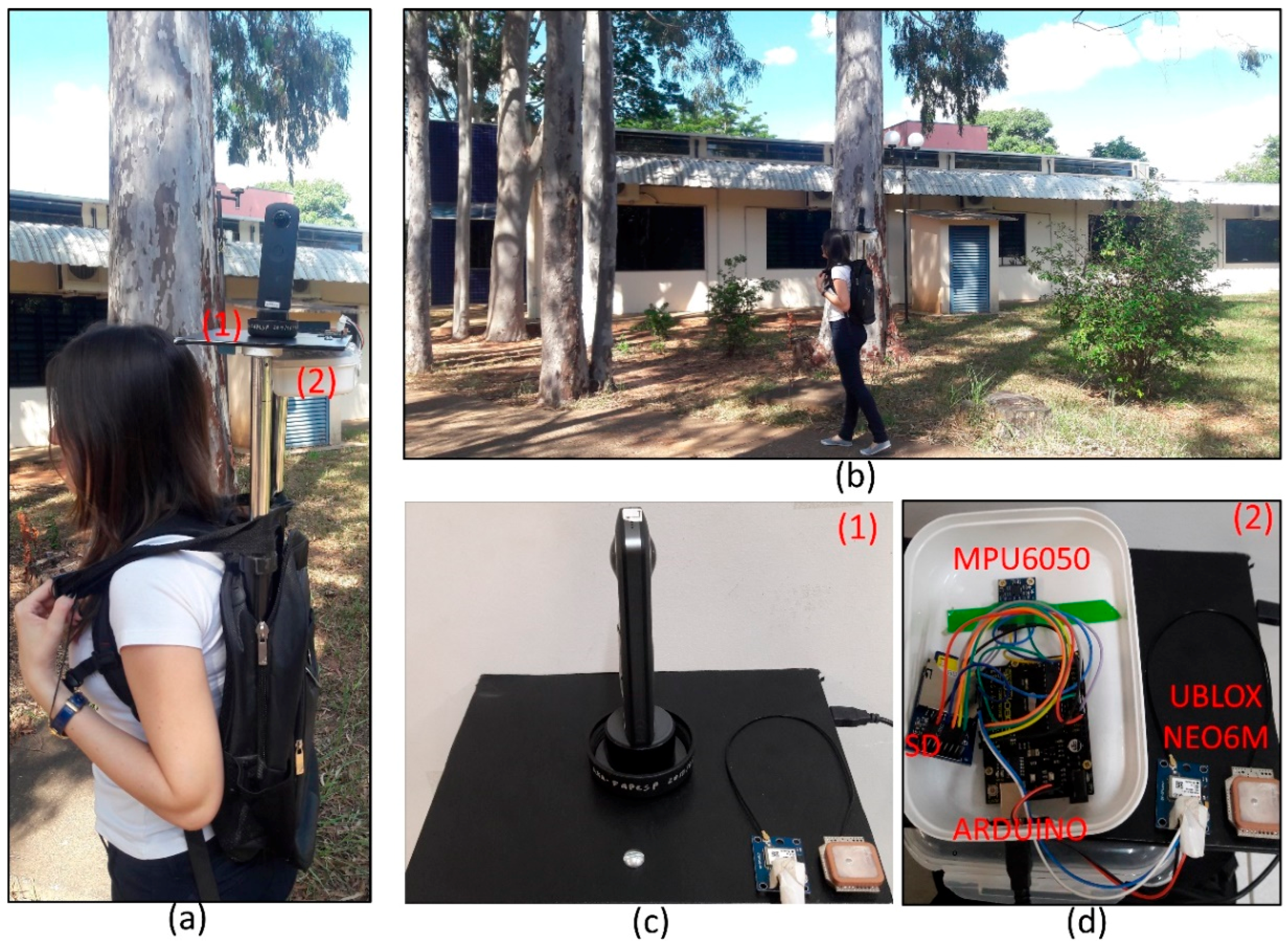
3.1. Data Sets

The experimental assessments of the proposed method were performed in a test area located at the São Paulo State University (UNESP) campus of Presidente Prudente, Brazil (Figure 5). Data sets were acquired using a low-cost personal mobile terrestrial system, known as PMTS [20], which is composed by the poly-dioptric system Ricoh Theta S [21,22] and off-the-shelf navigation systems embedded in a backpack platform (Figure 6). Figure 6 depicts the PMTS used for a mobile mapping acquisition, aiming a SfM solution.

The Ricoh Theta S is composed of two fisheye lenses with a field of view greater than 180° (~210°; c ≈ 1.43 mm) in a back-to-back position and two complementary metal oxide semiconductor (CMOS) sensors (1/2.3’’) with 7.2 megapixels on each side of the camera (Figure 6c). Aimed at dense acquisition for a SfM solution, Ricoh Theta S was used in video mode to acquire 29 dual-fisheye frames per second with a fisheye image resolution of 960 x 1080 pixels for each sensor and a 5 μm pixel size. Navigation data were collected using low-cost sensors (GPS receiver Ublox NEO-6M and IMU MPU 6050) integrated with an Arduino microprocessor (Figure 6d). The PMTS sensors were previous calibrated, integrated, and synchronized, providing a sequential data acquisition for each 1 second of survey [20]. Figure 6b shows an example of an operator carrying the PMTS. The relative accuracy between consecutive measurements was 0.08 m and 1° (1 s) for sensor position and attitude [22].

Dataset I was obtained from a controlled scene (indoor) composed of ArUco [30] coded targets with known coordinates, as shown in Figure 7a. This data set was initially used to assess the proposed method advantages and disadvantages because the image analysis is more controlled in artificial targets. A set of 5 omnidirectional images was acquired with the Ricoh Theta S arranged in a leveled tripod. The EOPs were estimated in a previous bundle adjustment, and errors (0.08 m and 1°) were added to simulate initial values similar to the PMTS navigation system. The pixel size in object space units (ground sample distance (GSD)) ranges between 4 and 6 mm (the approximate camera-to-object distance is 1.2 m from the central targets), and the image baseline varied between 1 and 4 m.

Dataset II was acquired in a forest area (Figure 7b) with the proposed low-cost PMTS [20]. A set of 77 omnidirectional images with EOPs from the navigation system (Figure 6d) was selected from the Ricoh Theta S video data to perform the experiments. The relative accuracies of the ROPs were 1° in attitude and 0.3 m in position because the GPS measurements were more heavily affected by multipath errors and signal obstruction inside of the forest areas. From this dataset, 5 images were selected for experiment I (Section 3.2) with an average pixel size in object space units of 1 cm and an image base ranging from 0.73 to 2.3 m.

Dataset III corresponds to a set of 57 omnidirectional images selected from the PMTS acquisition carried out in an urban area (Figure 7c) covered with sparse vegetation areas of eucalyptus trees, ground vegetation (grass and bush), small buildings, and urban objects (e.g., traffic signals). A set of 5 images were selected in this area for experiment I (Section 3.2) and 12 images for experiment II (Section 3.3). These images have a pixel size in object space units ranging between 2 and 5 cm and an image base ranging from 0.74 to 3.15 m. Initial navigation data were obtained with an average accuracy of 1° and 0.3 m.

Figure 7 presents a sample of the omnidirectional and rectified images from data sets I, II, and III.

3.2. Experiment I: Comparison of Omnidirectional Matching Approaches Based on SIFT

This experiment was designed to compare and discuss the performance of the three research trends (Section 1) on omnidirectional image matching (A, B, and C), considering data sets I to III, and to analyze the feasibility of these approaches for close-range applications. The proposed method (SIFT_RFS) detailed in Section 2 (approach C) was compared with the following approaches:

Approach A (SIFT_RTF): The standard SIFT method [5] was applied in fisheye images geometrically converted to perspective images (rectified), as presented in Figure 5. The rectified fisheye images were generated as presented and implemented in Reference [3].

Approach B: pSIFT [1] was used to compare the proposed method with an omnidirectional interest operator for close range applications. This method is a SIFT extension that uses the original omnidirectional images and considers a stereographic projection as an approximation for the diffusion on the sphere, which was previously developed and tested for outdoor sensor location [1]. This approach was implemented in MATLAB scripts.

In this experiment, for all three data sets, a threshold of 0.4 was selected for SIFT_RFS and pSIFT applied on the original fisheye images because of the large scale variation. Because radiometric distortions are higher in rectified images, a threshold of 0.6 was empirically defined for standard SIFT on the rectified fisheye images (SIFT_RTF), with a minimum number of matches per pair of images (>6). In each data set, image matching was performed with SIFT_RTF, SIFT_RFS, and pSIFT applied to 5 consecutive images, which represents 10 sequential pairs of images (1-5, 2-5, 3-5, and 4-5) to be analyzed. The range of 1 to 5 sequential images was empirically determined to avoid exhaustive matching by considering the maximum base distance (baseline) between images obtained with the PMTS, which enables the detection of a minimum number of matches (>6) for a bundle adjustment. Because of the large field-of-view of the fisheye images (≈210°), the overlap between images (1 to 5) is almost 100%. However, the main limitation is the drastic change of target appearance according to the baseline increasing, especially for the targets close to the sensor. Therefore, the detection rate decreased as a function of the baseline between images. This range can change according to the environment or the speed of platform displacement, which needs to be pre-evaluated.

3.3. Experiment II: Sensor Position and Attitude Estimation

The applicability of the proposed method (SIFT_RFS) for CRP applications was tested with a postprocessing approach that considered the set of matches obtained with SIFT_RFS as observations in a global bundle adjustment to estimate the EOPs and 3D ground coordinates for the sequential acquisition in dataset III. A set of 12 images from dataset III was used, which corresponds to 10 m of PMTS trajectory. The bundle adjustment was implemented (C/C++ language) based on the unified approach to the least squares method [26] using the equidistant fisheye lens equations (Ricoh Theta S model) as a mathematical model [21].

A standard deviation of 1.5 pixels was assumed for image observations from SIFT_RFS in both components, i.e., column and row (c, r). The 3D coordinates of eight ground control points (GCPs) and six checkpoints were obtained from a high-accuracy terrestrial laser point cloud measured in the same test area using the Leica ScanStation P40. A standard deviation of 0.05 m was set for GCPs in the bundle adjustment. The initial values for the EOPs were applied with standard deviations of 0.5 m for the camera position (X₀, Y₀, and Z₀) and 10° for the attitude parameters (ω, ϕ, and κ). The IOPs were considered as absolute constraints, which were estimated in a previous camera calibration process [21].

3.4. Performance Assessment

The detection rate (number of points detected), number of successful matches (location correctness), repeatability (defined in this paper as the number of conjugate points detected in sequential pair of images), and the geometric distribution of points over the images were considered as criteria for performance assessment in Experiment I. These criteria were defined because they are closely related to the accuracy of estimated values for the sensor exterior orientation (Experiment II).

In Experiment I, the matches were manually checked by three independent operators, and matching errors greater than 3 pixels were considered erroneous. Repeatability was estimated by computing the number of image pairs in which the same point was successfully matched. The geometric distribution was assessed using the number of matches located in the four quadrants of an image. The standard SIFT performance in omnidirectional and perspective images was considered as a reference to quantify the improvements achieved with approaches A, B, and C. To this end, SIFT was applied in the original fisheye images from all data sets. In addition to the fisheye images, a set of perspective images was acquired using a perspective digital camera (Nikon D3100, 4608 × 3072 pixels) in dataset III with a B/D (base-to-distance ratio) geometry similar to the omnidirectional images.

In Experiment II, the residuals in the image coordinates obtained in the bundle adjustment and the a posteriori standard error of unit weight (sigma naught) were used to assess the quality of match locations. The estimated precision (standard deviations) of the EOPs was analyzed based on average values estimated from the covariance matrix. Finally, the accuracies achieved with the bundle adjustment on the ground points were assessed by considering the discrepancies between the estimated and directly measured coordinates of the checkpoints.

4. Results and Discussion

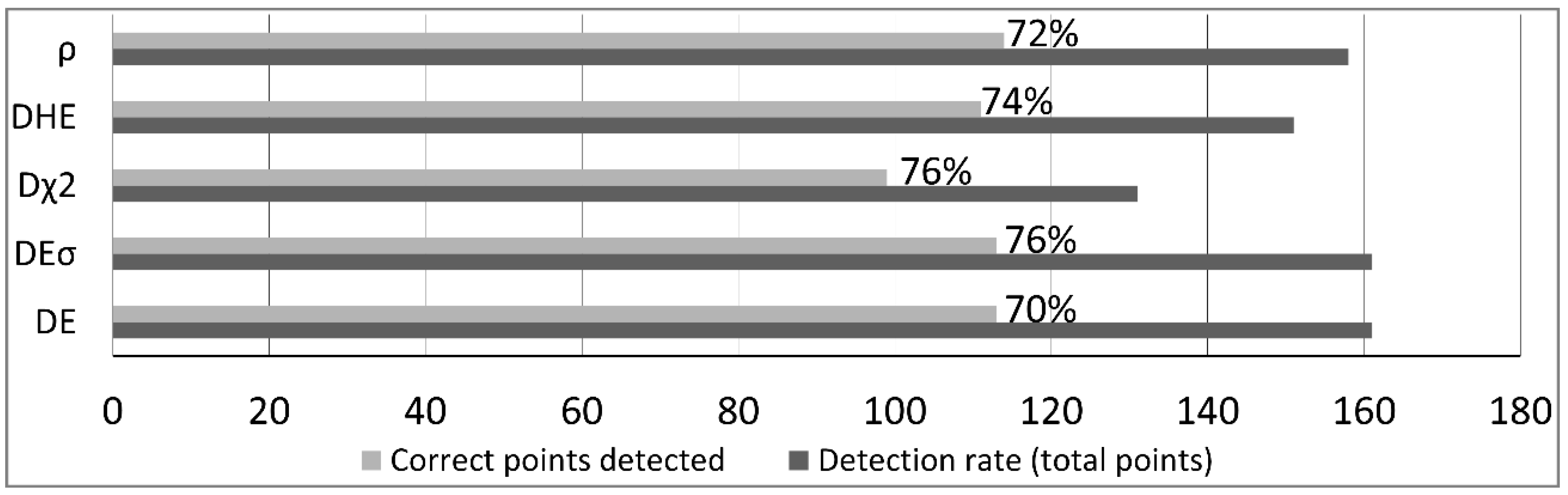
4.1. Preliminary Assessment of Interest Operators on Fisheye Images

FBM techniques, such as SIFT, FAST (features from accelerated segment test), SURF, and MOPS (multi-scale oriented patches), had been extensively tested and analyzed for perspective images. However, only few studies discussed the applicability of these operators in omnidirectional images [13,31]. In order to verify the performance of these interest operators for fisheye images in close range applications, a triplet of images from dataset III was selected. These four operators were applied in the triplet of fisheye images using MATLAB functions for SIFT, SURF, and FAST, and the free software ImageJ for MOPS. A threshold of 0.5 for image matching acceptance was employed. The detection rate (number of points detected) and number of successful matches (location correctness) were considered as performance criteria.

Table 1. SIFT, speeded-up robust features (SURF), features from accelerated segment test (FAST), and multi-scale oriented patches (MOPS) performance (detection rate and location correctness) in Ricoh Theta S fisheye images.

Interest Operator	Detection Rate	Location Correctness	Mismatches
SIFT	164	70% (114/164)	30% (50/164)
SURF	155	63% (98/155)	37% (57/155)
FAST	59	64% (38/59)	36% (21/59)
MOPS	123	14% (19/123)	86% (104/123)

shows the number of total points detected and the percentage of correct matches and mismatches for each standard SIFT, SURF, FAST, and MOPS algorithm applied for the triple of Ricoh Theta S fisheye images.

From this data set, SIFT obtained the most successful detection rate among the four operators with 70% of correct matches, while FAST and SURF presented 64% and 63%, respectively, of location correctness. The less favorable performance was obtained with the MOPS operator (14%), in which the mismatch is higher than the correct rate. In summary, SIFT and SURF presented similar results as in Reference [31]. However, considering the evaluated data set, some advantages and disadvantages can be noted. For instance, SURF was at least four times faster than SIFT. On the other hand, SIFT provided a higher number of matches and a better location accuracy than SURF on Ricoh Theta S fisheye images. Furthermore, the points distribution was more homogeneous when using SIFT. These results are in line with previous works [12,13], that also applied SIFT in omnidirectional images from outdoor scenarios with satisfactory results. This preliminary analysis motivated the SIFT choice in this study.

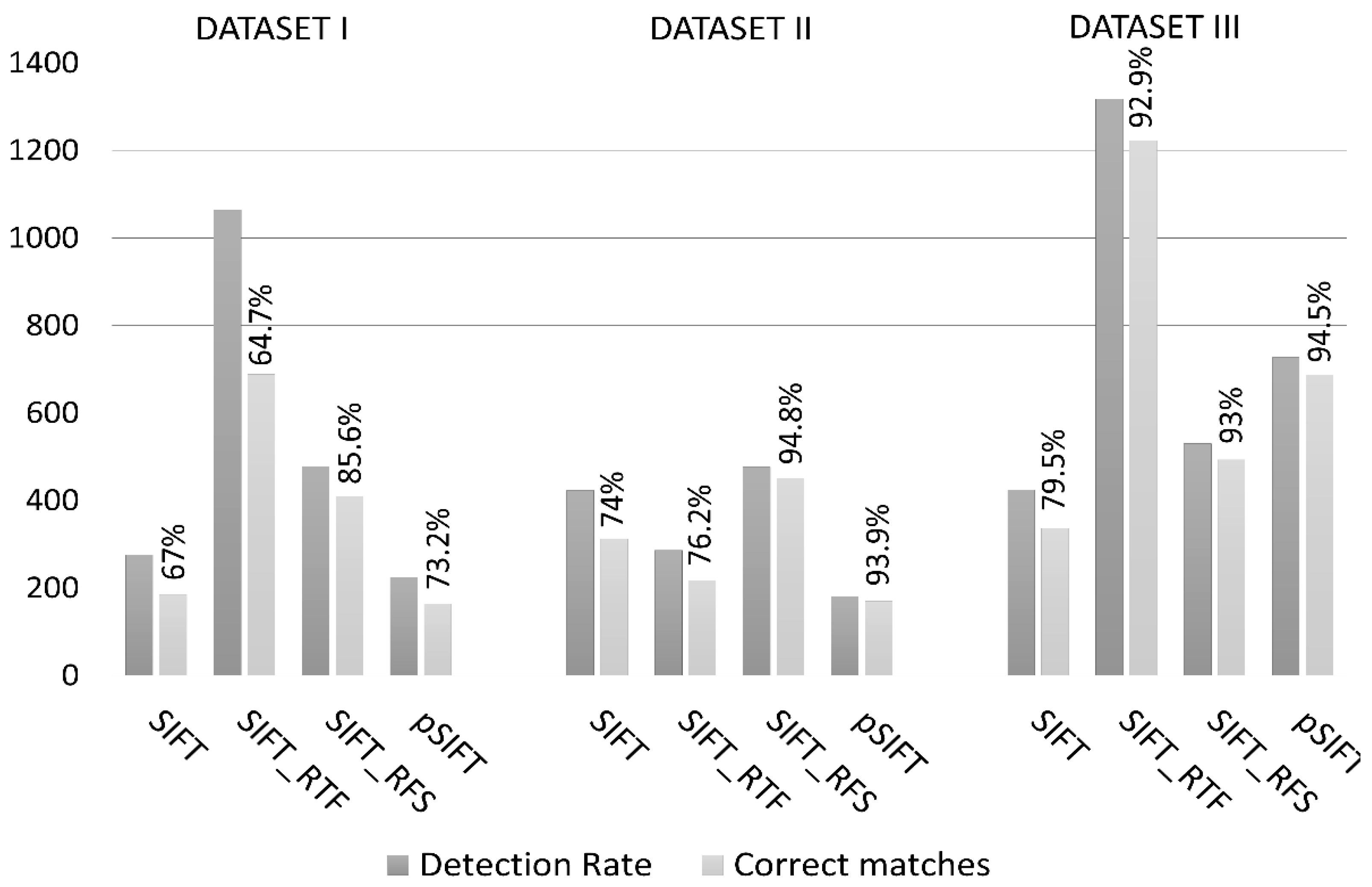
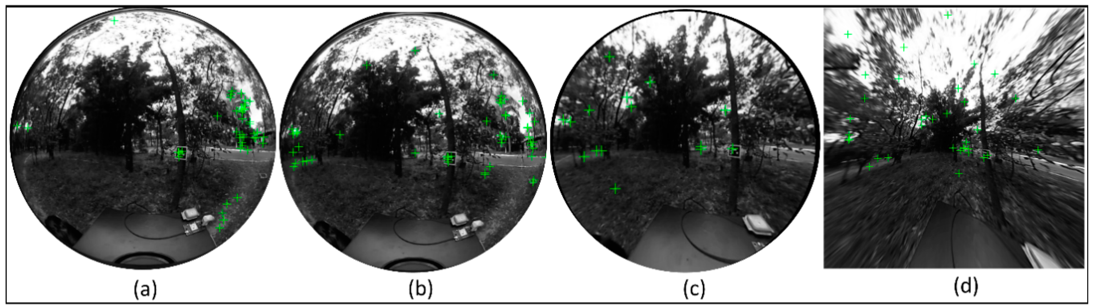
4.2. Assessment of Omnidirectional Matching Approaches (Experiment I)

4.2.1. Detection Rate and Location Correctness

Figure 8 summarizes the detection rate and successful matching rates (location accuracy in percentage) obtained from 10 pairs of fisheye images with standard SIFT, SIFT_RTF (approach A), pSIFT (approach B), and SIFT_RFS (approach C) for data sets I to III.

The main challenge in terms of location correctness was nonuniqueness matches due to repetitive patterns. Although approach A (SIFT_RTF) had a higher detection rate (Figure 8), the image projection to a plane introduced radiometric artifacts, mainly caused by illumination variations and nonstatic environments such as forests (data set II). Thus, higher thresholds for matching acceptance were required for SIFT_RTF, which enhanced the similarity between different targets, thus augmenting the ambiguity problem and resulting in the lowest location correctness among the three approaches.

The approaches that worked with the original fisheye images presented more consistent results. pSIFT (approach B) obtained a detection rate similar to that of standard SIFT but with an improvement of 6.2% in correctness on data set I. Better results were obtained with SIFT_RFS (approach C). Improvements of 73% in terms of number of detected points and of 18.6% for correct matches were obtained with SIFT_RFS in the same dataset compared with the standard SIFT on fisheye images. For dataset II, SIFT_RFS and pSIFT presented compatible results in terms of location correctness with improvements of 20.8% and 19.9%, respectively, compared with the standard SIFT. However, SIFT_RFS achieved a higher detection rate.

In summary, the results from data sets I (indoor) and II (forest) demonstrated that the proposed search space reduction minimized the image-matching ambiguity problem and the impact of omnidirectional image deformation. Therefore, SIFT_RFS is a good alternative in areas with repetitive patterns and homogeneous texture, which is often the case in outdoor applications of photogrammetry. The results are consistent with the discussions presented by Valiente et al. [18], who also showed that the epipolar geometry constraint reduced false matches by establishing a limited feature search space and improved sensor location in indoor data sets. It should be noted that the epipolar curve is only a geometric restriction, which does not assure a correct match. Most of the false matches detected with SIFT_RFS were located in the same epipolar curve or were occluded, which is an intrinsic characteristic of this approach.

Dataset III offers a different awareness (Figure 8). SIFT_RFS (93%) presented similar location correctness than SIFT_RTF (93%) and pSIFT (94,5%). However, in terms of detection rate, the geometrically rigorous approaches A (SIFT_RTF) and B (pSIFT) outperformed approach C (SIFT_RFS). The detection rate is an important criterion because the sensor location and attitude (EOPs) can be better solved with a higher number of matched points [18]. The larger the number of conjugated points, the higher the degrees of freedom will be in the bundle adjustment and the computation time.

Considering the standard SIFT performance in data set III as a reference (SIFT_PERSPECTIVE), a location correctness of 97% was obtained in the perspective images acquired with a perspective digital camera (Nikon D3100), which illustrates the impact of fisheye image distortions on SIFT efficiency (SIFT_FISHEYE, 79%), as summarized in

Table 2. Summarized results of SIFT for data set III.

Method	Detection Rate (Total/Corrected Points)	Successful Matching Rate
SIFTFISHEYE	424/337	79.5%
SIFTPERSPECTIVE	858/832	97%
SIFTRFS	530/493	93%

. SIFT performance was reduced by approximately 20% for fisheye images (SIFT_FISHEYE) compared with perspective images (SIFT_PERSPECTIVE). An increased number of false matches in non-perspective images was also noted by Scaramuzza et al. [12] using a catadioptric system. The three approaches (A, B, and C) based on SIFT for fisheye images presented successful matching rates superior to 90% in data set III (Figure 8), thus improving the interest operator performance and partially overcoming the SIFT limitations. The results obtained for analysis of the detection rate and location correctness show the relevancy of introducing modifications compatible with fisheye geometry.

4.2.2. Repeatability

The repeatability performance criterion is the main limitation of the proposed method (SIFT_RFS, approach C) because the interest points are located with standard SIFT. According to Lowe [5], an average repeatability of 80% was obtained for key point detection and final matching with SIFT for a perspective pair of images with viewpoint rotation (affine distortion) of less than 30°. Repeatability is significantly reduced when the viewpoint rotation is increased. For instance, viewpoint rotations greater than 50° result in a repeatability of approximately 40% [5]. A similar aspect change occurs from image to image in the omnidirectional case, thus directly affecting SIFT performance. The repeatability assessment presented by Cruz et al. [8] showed a mean repeatability of 39% for standard SIFT in omnidirectional images. The experiments performed in References [5,8] consider the stability between key point generation in the same pair of images computationally rotated to simulate different points of view. This analysis was extended to real data sets to assess SIFT_RFS, SIFT_RTF, and pSIFT for outdoor CRP applications.

In this experiment, the viewpoint rotation between fisheye images changes according to the Ricoh Theta S point of view during PMTS acquisition. Therefore, the viewpoint rotation increases as a function of the base between image pairs. The repeatability was computed for 10 pairs of images in data set III. Repeatability values of 13% were obtained with SIFT_RFS (70/528 points) and pSIFT (97/727 points), against an average repeatability of 17% (235/1307 points) for approach A (SIFT_RTF). Methods, such as SIFT_RTF, which applied SIFT in the wide-angle images converted to a geometrically corrected perspective image, presented better results in terms of repeatability because the appearance of the target is more preserved along the PMTS acquisition. Thus, the scale invariance property required by SIFT is more constant.

Despite this disadvantage, the number of consecutive repeated points detected in the sequential fisheye images with SIFT_RFS are considered acceptable for EOP estimation in a bundle adjustment (Experiment II). The repeatability of key-point detection can be improved, whereas, it directly increases as a function of the standard deviation (σ) of the Gaussian function [5] and the acceptance threshold for descriptor comparison [8]. However, a cost exists for use of a large σ in terms of efficiency [5] and a large threshold in terms of location correctness [8], thus requiring further assessments to establish optimal values.

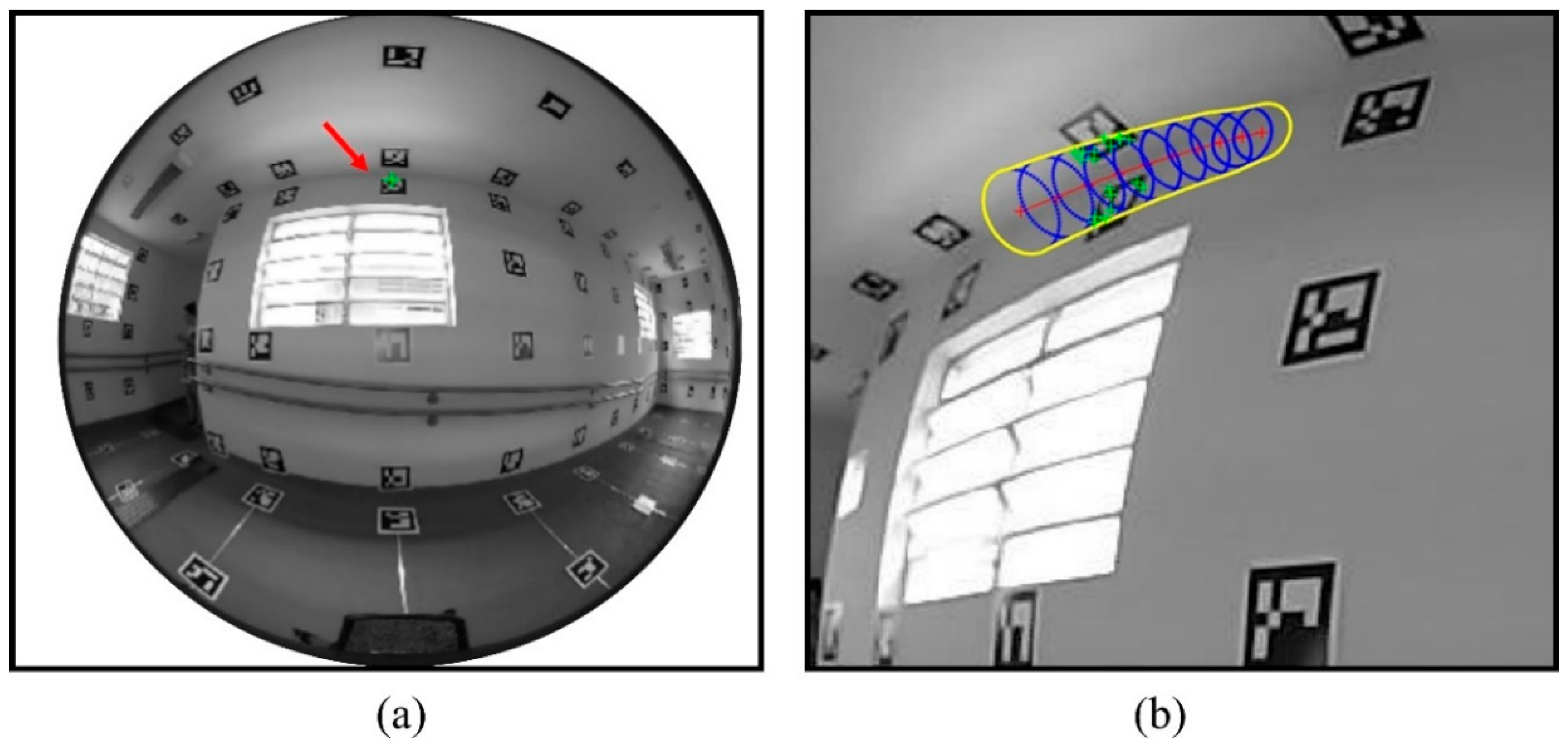
4.2.3. Geometric Distribution

Another consequence of scale and perspective variations in fisheye images for standard SIFT is the weak geometry of point distribution. Figure 9 presents examples of match distributions in a fisheye image from dataset II obtained with standard SIFT (a), SIFT_RFS (b), pSIFT (c), and SIFT_RTF (d).

Because the SIFT key points were selected based on their stability [5], many matches were selected in the fisheye image border (Figure 9a). These outcomes occur because targets far from the sensor have less variation in scale, viewpoint rotation and orientation during image acquisition along the PMTS trajectory, and thus their appearance changes less than that of points near the sensor. Point distribution were improved relative to standard SIFT using the three approaches. Considering all data sets, better point distributions were obtained with approaches A and B (SIFT_RTF and pSIFT), as depicted in Figure 9 for dataset II, because the point extraction processes are geometrically compatible.

The geometric distribution of the matched points in the block of images (tie points in the bundle adjustment) directly affects the EOP estimation, especially the attitude angles due to B/D geometry. B/D geometry is particularly challenging when using a fisheye lens because the number of point matches decreases as a function of the baseline. This difficulty increases in close-range applications because significant changes in the target aspect and illumination in a sequence of images are more likely to occur, especially if using mobile platforms. Therefore, in certain cases, a pair of images with optimal B/D value (≈1) does not supply a suitable number of matches. This problem was also discussed in References [1,9] using interest operators for omnidirectional images (approach B) based on SIFT. As alternative for FBM, some recent works have proposed the application of deep learning methods, such as the convolutional neural network (CNN), for automatic feature extraction (deep matching) [32], which also have shown high potential for image matching under strong distortions such as in fisheye images [33,34].

As a concluding comment in this section, the results from datasets I, II, and III show that image-matching performance was strongly related to the dataset environmental features, mostly in CRP applications, which can influence location correctness, repeatability, and the geometric distribution.

4.3. Sensor Pose and 3D Ground Coordinates Estimative (Experiment II)

The matches obtained with the proposed method (SIFT_RFS) in 12 images from dataset III were used in Experiment II with the goal of estimating the EOPs and ground coordinates of tie points in a global bundle block adjustment. The challenges in determining the EOPs from omnidirectional systems include accuracy of the image point measurements and their geometric distribution. Automatic image observations in nonstatic environments such as vegetation areas can select nonstable features such as tree leaves, shadows and clouds, which hinder the convergence of the solution, mainly when small displacements occur. These points determined in the matching step with large displacements were identified and removed by analyzing the image coordinate residuals in the x and y directions. With respect to the geometric distribution of the observations, the 3D coordinates of the detected image points aligned with the PMTS trajectory (infinity points) cannot be estimated because the intersection of the rays vanish to infinity [35]. Therefore, these points can be removed automatically, considering the angles formed between the bundles of rays (approaching zero). After observation filtering, a set of 203 match points was used (406 image points and 812 equations). The final root mean square error (RMSE) of the image coordinate residuals obtained in the bundle adjustment process was 1.3 pixels, with the a posteriori standard error of the unit weight (sigma naught) of 0.42 pixels. This result is compatible with the SIFT location accuracy.

The average values of the estimated standard deviations of the exterior orientation angles omega (σ_ω), phi (σ_ϕ), and kappa (σ_κ), and the camera perspective center position (σ_X0, σ_Y0, and σ_Z0) for all images obtained from the covariance matrix are presented in

Table 3. Estimated standard deviation of the exterior orientation parameters: Omega (σ_ω), phi (σ_ϕ), and kappa (σ_κ) in degrees and camera perspective center in meters.

σω (°)	σϕ (°)	σκ (°)	σX0 (m)	σY0 (m)	σZ0 (m)
0.37	0.21	0.39	0.037	0.037	0.041

. Overall, the EOPs were estimated with standard deviations of 0.3° and 4 cm for the sensor attitude and position, respectively.

Table 4. Statistics: Average ($\overline{\mathrm{x}}$), standard deviation (σ), and root mean square error (RMSE) of the checkpoints in East (E), North (N), and height (h) coordinates.

Statistics	E (m)	N (m)	h (m)
$\overline{\mathrm{x}}$	−0.117	−0.071	0.035
σ	0.097	0.069	0.101
RMSE	0.113	0.095	0.091

presents the statistics, including the average ($\overline{\mathrm{x}}$), standard deviation (σ), and RMSE of the discrepancies between the six checkpoints 3D coordinates measured in a laser point cloud (reference) and the estimated coordinates after bundle adjustment. The 3D terrain coordinates (E, N, and h) of the points detected with SIFT_RFS (tie points) were estimated with an average planimetric accuracy of 23 cm and a height accuracy of 12 cm, which can be considered compatible with the Ricoh Theta S image resolution.

5. Conclusions

We proposed a new recursive search space method for fisheye image matching (SIFT_RFS) for close range photogrammetry (CRP) applications. As proposed, the reduction of the search space can be easily implemented and reproduced for SfM solutions. Future work combining the reduction of the search space for fisheye images with other interest operators such as SURF and pSIFT can be performed, aiming new solutions for SfM approaches based on omnidirectional images. The proposed method for epipolar line estimation is an alternative to conventional implementations for omnidirectional images. The introduction of a geometric constraint supplied compatible results in real data challenges relative to other geometrically rigorous approaches such as SIFT_RTF and pSIFT, which require higher implementation efforts. For instance, SIFT_RFS improved the results in areas with repetitive patterns, whereas SIFT_RTF and pSIFT outperformed SIFT_RFS in terms of point geometric distribution. Studies focusing on the optimization of FBM implementation and a rigorous time processing analysis for fisheye images are suggested as future works.

The applicability of low-cost GNSS/IMU sensors for outdoor application with integrated sensor orientation (ISO) methodologies can be improved using approaches based on the relative orientation parameters, such as SIFT_RFS, thus enabling more flexible mobile mapping systems. Low-cost systems are noise-sensitive, which can result in a low absolute accuracy. However, the relative measurements are more stable because certain sources of error are mitigated, such as inaccuracies in the mounting parameters and systematic errors in the GNSS position and the attitude computed from IMU data. The relative positions and angles between GNSS/IMU observations can be used as relative constraints to improve sensor location estimation in the bundle adjustment. In this paper, the EOPs were estimated in postprocessing bundle adjustment with an average accuracy of four centimeters. Real-time trajectory estimation using SIFT_RFS is recommended as a complement to assessment of the proposed method in CRP applications.

References

1. Hasen, P.; Corke, P.; Boles, W. Wide-angle visual feature matching for outdoor localization. Int. J. Robot. Res. 2010, 29, 267–297. [Google Scholar] [CrossRef]
2. Hasen, P.; Corke, P.; Boles, W.; Daniilidis, K. Scale-invariant features on the sphere. In Proceedings of the IEEE 11th International Conference on Computer Vision, Rio de Janeiro, Brazil, 14–21 October 2007; pp. 1–8. [Google Scholar]
3. Tommaselli, A.M.G.; Berveglieri, A. Automatic orientation of multi-scale terrestrial images for 3D reconstruction. Remote Sens. 2014, 6, 3020–3040. [Google Scholar] [CrossRef]
4. Chuang, T.Y.; Perng, N.H. Rectified feature matching for spherical panoramic images. Pers 2018, 84, 25–32. [Google Scholar] [CrossRef]
5. Lowe, D.G. Distinctive image features from scale-invariant keypoints. Int. J. Comput. Vis. (IJCV) 2004, 60, 91–110. [Google Scholar] [CrossRef]
6. Daniilidis, K.; Makadia, A.; Bulow, T. Image processing in catadioptric planes: Spatiotemporal derivatives and optical flow computation. In Proceedings of the IEEE Third Workshop on Omnidirectional Vision, Copenhagen, Denmark, 2 June 2002; pp. 3–10. [Google Scholar] [CrossRef]
7. Bulow, T. Spherical diffusion for 3D surface smoothing. IEEE Trans. Pattern Anal. Mach. Intell. 2004, 26, 1650–1654. [Google Scholar] [CrossRef] [PubMed]
8. Cruz-Mota, J.; Bogdanova, I.; Paquier, B.; Bierlaire, M.; Thiran, J.P. Scale invariant feature transform on the sphere: Theory and applications. Int. J. Comput. Vis. (IJCV) 2012, 98, 217–241. [Google Scholar] [CrossRef]
9. Arican, Z.; Frossard, P. Scale-invariant features and polar descriptors in omnidirectional imaging. IEEE Trans. Image Process. 2012, 21, 2412–2423. [Google Scholar] [CrossRef] [PubMed]
10. Lourenco, M.; Barreto, J.; Vasconcelos, F. sRD-SIFT: Keypoint Detection and Matching in Images with Radial Distortion. IEEE Trans. Robot. 2012, 28, 752–760. [Google Scholar] [CrossRef]
11. Puig, L.; Guerrero, J.; Daniilidis, K. Scale space for camera invariant features. IEEE Trans. Pattern Anal. Mach. Intell. 2014, 36, 1832–1846. [Google Scholar] [CrossRef] [PubMed]
12. Scaramuzza, D.; Siegwart, R. Appearance-guided monocular omnidirectional visual odometry for outdoor ground vehicles. IEEE Trans. Robot. 2008, 24, 1015–1026. [Google Scholar] [CrossRef]
13. Valgren, C.; Lilienthal, A.J. SIFT, SURF & seasons: Appearance-based long-term localization in outdoor environments. Robot. Auton. Syst. 2010, 58, 149–156. [Google Scholar] [CrossRef]
14. Kraus, K. Photogrammetry—Geometry from Images and LASER Scans, 2nd ed.; Walter de Gruyter: Berlin, Germany, 2007; pp. 1–459. [Google Scholar]
15. Svoboda, T.; Pajdla, T.; Hlaváč, V. Epipolar geometry for panoramic cameras. In Proceedings of the European Conference on Computer Vision, Berlin, Germany, 2–6 June 1998; pp. 218–231. [Google Scholar]
16. Bunschoten, R.; Krose, B. Range Estimation from a Pair of Omnidirectional Images. In Proceedings of the IEEE-ICRA, Seul, Korea, 21–26 May 2001; pp. 1174–1179. [Google Scholar]
17. Abraham, S.; Forstner, W. Fish-eye-stereo calibration and epipolar rectification. ISPRS Prs 2005, 59, 278–288. [Google Scholar] [CrossRef]
18. Valiente, D.; Gil, A.; Reinoso, Ó.; Juliá, M.; Holloway, M. Improved omnidirectional odometry for a view-based mapping approach. Sensors 2017, 17, 325. [Google Scholar] [CrossRef] [PubMed]
19. Tommaselli, A.M.G.; Tozzi, C.L. A recursive approach to space resection using straight lines. Pers 1996, 62, 57–66. [Google Scholar]
20. Campos, M.B.; Tommaselli, A.M.G.; Honkavaara, E.; Prol, F.S.; Kaartinen, H.; Issaoui, A.E.; Hakala, T. A Backpack-Mounted Omnidirectional Camera with Off-the-Shelf Navigation Sensors for Mobile Terrestrial Mapping: Development and Forest Application. Sensors 2018, 18, 827. [Google Scholar] [CrossRef] [PubMed]
21. Campos, M.B.; Tommaselli, A.M.G.; Marcato-Junior, J.; Honkavaara, E. Geometric model and assessment of a dual-fisheye imaging system. Photogramm. Rec. 2018, 33, 243–263. [Google Scholar] [CrossRef]
22. Hellwich, O.; Heipke, C.; Tang, L.; Ebner, H.; Mayr, W. Experiences with automatic relative orientation. In Proceedings of the ISPRS symposium: Spatial Information from Digital Photogrammetry and Computer Vision, Munich, Germany, 5–9 September 1994; pp. 370–379. [Google Scholar] [CrossRef]
23. Zhang, Z. Determining the epipolar geometry and its uncertainty: A review. Int. J. Comput. Vis. (IJCV) 1998, 27, 161–195. [Google Scholar] [CrossRef]
24. Hughes, C.; Denny, P.; Jones, E.; Glavin, M. Accuracy of fish-eye lens models. Appl. Opt. 2012, 49, 3338–3347. [Google Scholar] [CrossRef] [PubMed]
25. Schneider, D.; Schwalbe, E.; Maas, H.G. Validation of geometric models for fisheye lenses. Isprs Prs 2009, 64, 259–266. [Google Scholar] [CrossRef]
26. Mikhail, E.M.; Ackermann, F.E. Observations and Least Squares, 1st ed.; IEP—A Dun-Donnelley Publishers: New York, NY, USA, 1976; pp. 1–497. [Google Scholar]
27. Pope, A.J. The Statistics of Residuals and the Detection of Outliers, NOAA Technical Report; National Geodetic Survey: Rockville, MD, USA, 1976; Tech. Rep. NOS-65-NGS-1. [Google Scholar]
28. Arandjelovic, R.; Zisserman, A. Three things everyone should know to improve object retrieval. In Proceedings of the IEEE-CVPR, Providence, RI, USA, 16–21 June 2012; pp. 2911–2918. [Google Scholar]
29. The MathWorks: Statistics and Machine Learning Toolbox™ User’s Guide. Version 11.4-2018b, Sep. 2018. Available online: https://www.mathworks.com/help/pdf_doc/stats/stats.pdf (accessed on 5 November 2018).
30. Garrido-Jurado, S.; Muñoz-Salinas, R.; Madrid-Cuevas, F.J.; Marín-Jiménez, M.J. Automatic generation and detection of highly reliable fiducial markers under occlusion. Pattern Recognit. 2014, 47, 2280–2292. [Google Scholar] [CrossRef]
31. Murillo, A.C.; Guerrero, J.J.; Sagues, C. Surf features for efficient robot localization with omnidirectional images. In Proceedings of the IEEE-ICRA, Rome, Italy, 10–14 April 2007; pp. 3901–3907. [Google Scholar]
32. Merkle, N.; Luo, W.; Auer, S.; Müller, R.; Urtasun, R. Exploiting deep matching and SAR data for the geo-localization accuracy improvement of optical satellite images. Remote Sens. 2017, 9, 586. [Google Scholar] [CrossRef]
33. Deng, F.; Zhu, X.; Ren, J. Object detection on panoramic images based on deep learning. In Proceedings of the IEEE-ICCAR, Nagoya, Japan, 24–26 April 2017; pp. 375–380. [Google Scholar]
34. Zbontar, J.; LeCun, Y. Stereo Matching by Training a Convolutional Neural Network to Compare Image Patches. JMLR 2016, 17, 1–32. [Google Scholar]
35. Schneider, J.; Läbe, T.; Förstner, W. Incremental real-time bundle adjustment for multi-camera systems with points at infinity. ISPRS Arch. Photogramm. Remote Sens. Spat. Inf. Sci. 2013, 1, W2. [Google Scholar] [CrossRef]
Figure 1. Flow chart of the recursive search space method for fisheye image matching.
Remotesensing 11 01404 g001
Figure 2. Epipolar line estimation using the proposed method, in which an image point in the left image (pl) is projected to the object space (PI, PII,…,Pn) using the inverse collinearity condition on the sphere domain, and re-projected to the right image (pr) with the equidistant equations.
Remotesensing 11 01404 g002
Figure 3. (a) Interest point in the left-image (pl) and (b) search window in the right-image, in which the epipolar curve is shown in red, error ellipses in blue, the search window in yellow, and the selected scale-invariant feature transform (SIFT) keypoints in green.
Remotesensing 11 01404 g003
Figure 4. Detection rate and correct and incorrect points using the following metrics: Euclidean (DE), standardized Euclidean (D), chi-square (Dχ2), and Hellinger (DHE).
Remotesensing 11 01404 g004
Figure 5. Test area at São Paulo State University: Indoor (data set I), forest (data set II), and urban (data set III) scenes.
Remotesensing 11 01404 g005
Figure 6. Personal mobile terrestrial system (PMTS) for a sequential data acquisition: (a) PMTS imaging and navigation sensors, (b) PMTS carried by an operator in the test area (dataset III), (c) Ricoh Theta S camera, and (d) navigation sensors.
Remotesensing 11 01404 g006
Figure 7. Sample of omnidirectional and rectified images from the test areas: (a) data set I—indoor, (b) data set II—forest, and (c) data set III—urban scenes.
Remotesensing 11 01404 g007
Figure 8. Experiment I: Total of detection rate and location correctness of SIFT, SIFTRTF, pSIFT, and the proposed method SIFTRFS for indoor (data set I), forest (data set II), and urban (data set III) scenes.
Remotesensing 11 01404 g008
Figure 9. Experiment I: Example of match distribution for dataset II with (a) standard SIFT, (b) SIFTRFS, (c) pSIFT, and (d) SIFTRTF.
Remotesensing 11 01404 g009