Data Registration with Ground Points for Roadside LiDAR Sensors


1
Department of Civil and Environmental Engineering, University of Nevada, Reno, NV 89557, USA
2
School of Qilu Transportation, Shandong University, Jinan 250002, China
3
School of Economics and Management, Chang’An University, Xi’an 710064, China
*
Author to whom correspondence should be addressed.
Remote Sens. 2019, 11(11), 1354; https://doi.org/10.3390/rs11111354
Submission received: 6 May 2019
/
Revised: 27 May 2019
/
Accepted: 4 June 2019
/
Published: 5 June 2019
(This article belongs to the Section Urban Remote Sensing)
Abstract
:The Light Detection and Ranging (LiDAR) sensors are being considered as new traffic infrastructure sensors to detect road users’ trajectories for connected/autonomous vehicles and other traffic engineering applications. A LiDAR-enhanced traffic infrastructure system requires multiple LiDAR sensors around intersections, along with road segments, which can provide a seamless detection range at intersections or along arterials. Each LiDAR sensor generates cloud points of surrounding objects in a local coordinate system with the sensor at the origin, so it is necessary to integrate multiple roadside LiDAR sensors’ data into the same coordinate system. None of existing methods can integrate the data from roadside LiDAR sensors, because the extensive detection range of roadside sensors generates low-density cloud points and the alignment of roadside sensors is different from mapping scans or autonomous sensing systems. This paper presents a method to register datasets from multiple roadside LiDAR sensors. This approach innovatively integrates LiDAR datasets with 3D cloud points of road surface and 2D reference point features, so the method is abbreviated as RGP (Registration with Ground and Points). The RGP method applies optimization algorithms to identify the optimized linear coordinate transformation. This research considered the genetic algorithm (global optimization) and the hill climbing algorithm (local optimization). The performance of the RGP method and the different optimization algorithms was evaluated with field LiDAR sensors data. When the developed process can integrate data from roadside sensors, it can also register LiDAR sensors’ data on an autonomous vehicle or a robot.

1. Introduction
The new generation of transportation systems employ advanced communication technologies, such as 5G network [1]; dedicated short-range communication (DSRC) [2]; and sensing technologies, such as Light Detection and Ranging (LiDAR) and video sensors, to exchange each other’s real-time status and to understand the surrounding traffic environment. When autonomous vehicle platforms can achieve real-time detection and control, connected-vehicle technologies allow drivers/vehicles to “see” across buildings, over surrounding vehicles and other obstacles [3,4]. The advantages of connected vehicles rely on vehicle2x wireless communication, including but not limited to vehicle-to-vehicle, vehicle-to-infrastructure, and vehicle-to-other-road users. However, it is estimated that the full deployment of connected-vehicle equipment will take decades [5]. During this period, the traffic flow will include both the connected/autonomous vehicles and the unconnected road users who are “black spots” of the intelligent traffic systems. Without all users being sensed accurately, the benefits of connected vehicles and other advanced traffic systems will be limited.
Research has been started to enhance traffic infrastructures by deploying light detection and ranging (LiDAR) sensors on roadsides [6,7,8,9,10]. The roadside LiDAR sensors allow traffic infrastructures to sense the real-time high-accuracy trajectories of every vehicle/pedestrian/bicycle, so the system is not impacted by whether all road users share their real-time status. With the real-time data from roadside LiDARs, connected/autonomous vehicles know all the other road users without “black spots.” Traffic infrastructures can actively trigger traffic signals/warnings whenever they detect crash risks or changed traffic patterns. When the recent research efforts have developed and implemented the LiDAR data processing algorithms to extract high-resolution high-accuracy trajectories from roadside LiDAR data [7,8], a solution to integrate LiDAR data from different roadside sensors is needed. Each LiDAR sensor generates the 3D cloud points in a local coordinate system with the sensor at the origin. When LiDAR sensors are installed at an intersection or along an arterial, the data needs to be integrated by converting all LiDAR data into the same coordinate system. Incorporating LiDAR data from different scans or sensors, also called LiDAR data registration, has been studied for many years for mapping and autonomous vehicle/robots sensing [11,12,13]. 3D mapping scans an object from different viewpoints by rotating the object or moving scanners and then merging them into a complete model [14]. A point cloud from each LiDAR scan is in a local coordinate system so that the transformation of each view into the same coordinate system is needed. This process is called point cloud registration, and it is one of the critical problems in 3D reconstruction [15]. The general non-automated registration methods include manual registration, attaching markers onto the scanned object, and calibrating the movement between two scans in advance [15]. The automatic registration methods of 3D LiDAR scan can be classified into three types: point-based transformation model, line-based transformation model, and plane-based transformation model [16].
The spatial transformation of point clouds using point features can be established by a point-to-point correspondence and solved by least-squares adjustment. Besl and Mckay [17] conducted the foundation work of point-based automatic registration with the classical iterative closest point (ICP) algorithm. ICP starts with two point clouds and an initial guess for the transformation, and iteratively refines the transformation by repeatedly generating pairs of corresponding points in the point clouds and minimizing an error metric. However, the premise of using ICP for data integration was that the point clouds should be adequately close to each other [17]. Furthermore, the ICP lacks the ability to register the points with outliers and variable density [18]. Researchers also improved the ICP method to improve the computation efficiency and accuracy [18,19,20,21,22,23]. Wu et al. developed a revised partial iterative closest point algorithm (P-ICP) for LiDAR point clouds integration [19]. By selecting at least three representative points (usually corner points) from the two-point sets, the revised P-ICP can integrate the points within 0.2 s of time delay. The accuracy of the point registration has been greatly improved compared to that of the traditional ICP. The line-based automatic transformation comprises a 3D line feature transformed into another coordinate system that needs to be collinear with its counterpart. Stamos and Allen developed a method for range-to-range registration with manually selected 3D line features [24]. Stamos and Leordeanu developed an automated registration algorithm with corresponding line features [25]. A number of parameters were required to be calibrated in advance to customize the algorithm. The line-based registration was also used for registering LIDAR datasets and photogrammetric datasets [26]. The plane-based transformation is based on plane features [27,28,29]. The plane-based transformation methods formulated the problem of aligning two point clouds as a minimization of the squared distance between the corresponding surfaces. However, the above-mentioned three typical types of point registration methods require either large overlapping areas or clear features between two point clouds. Considering the massive deployment of the roadside LiDAR in the connect-vehicles in the future, only cost-effective LiDARs (8 beams or 16 beams) can be adopted. The extensive detection range of roadside LiDARs further decreased the overlapping areas and the point density. Therefore, the above-mentioned three methods could not be used for point registration of the roadside LiDARs.
The sensing system of autonomous vehicles requires the integration of multiple sensors such as LiDAR, video, radio detection and ranging (RADAR), short-wavelength infrared (SWIR), and global positioning system (GPS). The sensor fusion also requires the registration of LiDAR sensors’ data, or the registration of LiDAR data and other sensor data. The LiDAR-video integration normally builds separate visions, and the LiDAR feature extraction methods identify common anchor points in both [30,31]. For integrating multiple LiDAR sensors on a mobile platform, Cho et al. [32] treated six LIDARs in four planes as one homogeneous sensor, and analyzed sensor measurements using built-in segmentation and extracted features, like line segments or junctions of lines (“L”) shape [33].
All the reviewed registration methods in mapping and autonomous sensing only serve the scenarios with relative high-density cloud points, as shown in Figure 1a. Even the methods registering LiDAR data to images require many details of cloud points and pixels to achieve coordinate conversion. Some researchers on autonomous vehicle sensing systems use a board with a standard round hole or mark for registering multiple sensors. Researchers sometimes assume that LiDAR sensors on a vehicle platform are in a uniform coordinate system because the sensors are close to each other. These existing methodologies and assumptions do not apply to registering roadside LiDAR sensors for relative low-density cloud points caused by the wide detecting range and offset between laser beams of two sensors [34]. An example of the roadside LiDAR data is shown in Figure 1b. It differs noticably from Figure 1a.
This paper introduces a method particularly developed for registering roadside LiDAR sensors data into the same coordinate system. This approach innovatively integrates LiDAR datasets based on the 3D cloud points of the road surface and the selected 2D reference points, so the method is abbreviated as Registration with Ground and Points (RGP). The RGP method was developed for roadside sensors, and it can also be used to register the LiDAR sensors on a mobile platform such as an autonomous vehicle or a robot. The last step of the RGP method is to identify the parameters of linear coordinate transformation, offset-in-x, offset-in-y, offset-in-z, rotation-in-x, rotation-in-y, and rotation-in-z, with optimization algorithms. An objective function related to the 3D points of the ground surface and an objective function corresponding to the selected 2D reference points is defined. The two objective functions are further combined into a single objective function. The objective function has various local minimum/maximum values, so this research considered the genetic algorithm (GA) for global optimization and the hill climbing (HC) algorithm for local optimization for their advantages and disadvantages. The HC algorithm used an initial input that was estimated with a tool visualizing and customizing coordinate transformation. The performance of the RGP method and the optimization methods were evaluated with LiDAR data collected with two LiDAR sensors on different sides of a road.
This article is organized as the following: Section 2 presents the conception of coordinate transformation and the algorithm details of the RGP method. The performance evaluation results are demonstrated in Section 3. Section 4 provides the discussion of the influence of the proposed method on new transportation sensing systems and the extended research in the future. By the end, Section 5 summarizes the findings of this research.
2. Methodology
2.1. Coordinate Transformation
Linear transformations, as a type of coordinate transformation [35], convert points, lines, and planes in one coordinate to those in a second coordinate by a system of linear algebraic equations. A vector X in a 3-D coordinate system that has components Xj (xj, yj, zj), and in the primed-coordinate system the corresponding vector X’ has components Xi (xi, yi, zi) given by
Equations (1) and (2) give the general linear transformation of 3-D coordinate systems. This general linear form is divided into two constituents: the matrix A and the vector B. The vector B can be interpreted as a shift in the origin of the coordinate system. The elements Aij in the matrix A are the cosines of the angles between the axis of Xi and Xj. This is called the direction cosine. It needs to be noted that this linear conversion only includes the offsets in the x, y, and z axis and the rotations along x, y, and z axis, without changing the scales of x, y, and z. Therefore, a total of six parameters determine the required linear transformation (matrix A and vector B) for registering a LiDAR sensor dataset to another. To determine the six parameters: offset-in-x, offset-in-y, offset-in-z, rotation-in-x, rotation-in-y, and rotation-in-z, coordinates of two reference points in two coordinate systems are theoretically enough. The known coordinates of two reference points can be used to generate six equations, which are enough for solving the six transformation parameters. In the actual datasets, it is difficult to find accurate coordinates of a reference point in two coordinates. Therefore, optimization methods are commonly applied to identify the best linear transformation with two or more reference points, lines, or planes.
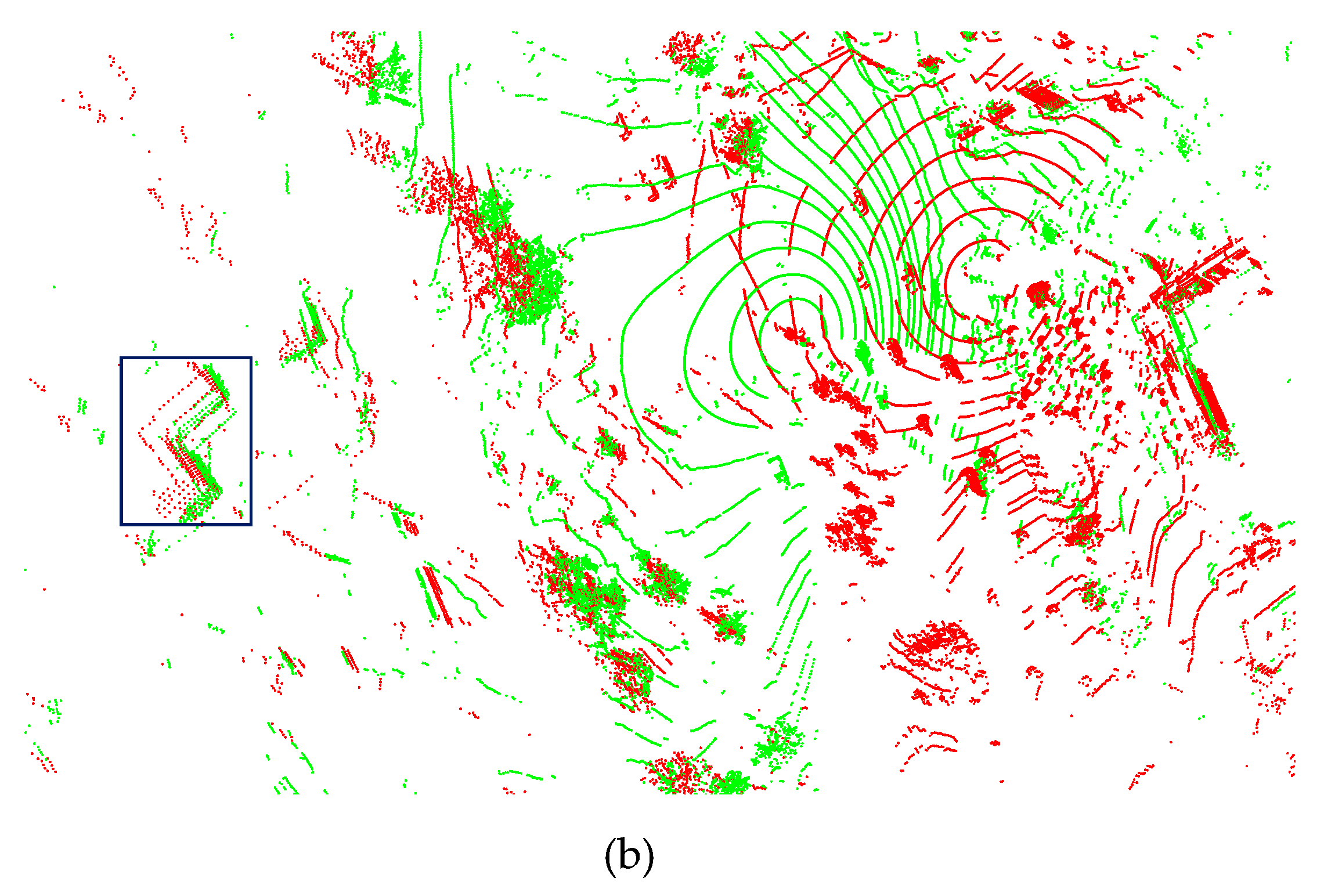
The reference features (points, lines, and planes) used in existing methods still need relatively accurate x, y, and z values of the same feature in two coordinates (overlap points). The high-resolution LiDAR cloud points, such as the ones used for mapping, can provide the required overlaps. For example, the LiDAR points of a building corner from the different stations can provide decent x, y, and z values of the same feature point in different station coordinates for high-resolution LiDAR cloud points. However, it is much more difficult or impossible to find the overlap x, y, and z values of the corresponding reference feature in different coordinates with the roadside sensors. Figure 2 presents the offsets of laser beams of two roadside LiDAR sensors in the z-axis. The two different colors mean the points are from the two different sensors. The points in the rounded rectangular box are of the same building, but the points of the different sensors are at different heights. In other words, the registered two LiDAR datasets may not have overlaps because of the z-axis offsets and the distance between the laser beams. This is the primary reason that the existing algorithms developed for mapping and autonomous sensing systems cannot register the roadside LiDAR data.
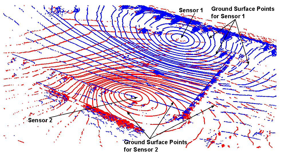
When it was not possible to find the coordinates of a reference feature in the two sensor coordinates, the authors innovatively used the ground surface LiDAR points of two roadside sensors. Though there is no guarantee of a building or object points from two sensors have overlap, there must be overlap points of the ground reflections in the two sensors’ data. The LiDAR points of ground surface are circles with the LiDAR sensor as the center. So, if two LiDAR datasets are correctly registered, the ground surface LiDAR points of the two sensors must have crossing points (overlaps), as shown in Figure 3. The problem of optimizing the linear transformation is that it needs to include an optimization function to minimize z difference of the overlap ground points (best match of the ground surface). With the ground surface points from the two LiDAR datasets, in each iteration, the converted coordinate is zoned into subareas with squares on the x-y surface. All ground surface LiDAR points are projected into the continuous x-y squares based on their x and y values. In each x-y square, the difference between the average z values of projected surface points of sensor 1 and the average z value of projected surface points of Sensor 2 (after the linear transformation) is calculated. If a square has only projected points from one sensor or has no projected points, this square is excluded from consideration. With the z difference calculated for all squares, the average z difference is calculated as an objective function.
The objective function to minimize the z difference of ground points of two sensors is described by Equations (3) and (4).
- F1—Objective function of minimum z difference of ground points of two sensors;
- z_diffi—z Difference of the x-y square i;
- zk_s1_i—z value of LiDAR point k of sensor 1 in square i;
- zl_s2_i—z value of LiDAR point l of sensor 2 (after linear transformation) in square i;
- xi_min—Minimum x boundary value of square i;
- xi_max—Maximum x boundary value of square i;
- yi_min—Minimum y boundary value of square i;
- xi_max—Maximum y boundary value of square i;
- xk_s1_i—x value of LiDAR point k of sensor 1 in square i;
- yk_s1_i—y value of LiDAR point k of sensor 1 in square i;
- xl_s2_i—x value of LiDAR point l of sensor 2 (after linear transformation) in square i;
- yl_s2_i—y value of LiDAR point l of sensor 2 (after linear transformation) in square i.
The test of optimization to minimize z difference of ground points found that the optimization result provided a good match of the ground surface of the two LiDAR datasets. However, this objective function is not sensitive enough to minimize offsets in x-axis and y-axis. For an accurate match in the x-direction and y-direction, two or more reference points are needed in the x-y 2D space.
It is impossible to find accurate coordinates related to the same reference feature in the two sensor datasets because of the z offsets, but x, y values corresponding to the same reference features (overlap points) can be found in the x–y space of the two sensor datasets. It is challenging to find the line or surface features from the two roadside datasets, because the sensors are distant from each other. In addition, when one sensor can detect a line or a surface of a building, the other sensor may not be able to catch the same surface or edge, as trees or obstacles around the two sensors are different. At least coordinates of two reference points in the two LiDAR datasets need to be identified to optimize the linear transformation for accurate registration in the x-axis and y-axis. More reference points can be used, if they are available, to improve the accuracy and reliability of the optimization. A semi-automatic method for the reference points detection can be found in reference [18].
The second objective function is to minimize the offsets of LiDAR points at the same point features in the x-y space. The objective function can be described by Equations (5) and (6).
- F2—The objective function of the minimum difference between the x,y coordinates of Sensor 1 and x,y coordinates of Sensor 2 after transformation at the selected reference point m;
- dm_s1_s2—Distance between the x,y coordinates of Sensor 1 and x,y coordinates of Sensor 2 after transformation at the selected reference point m;
- xm_s1—x value of LiDAR the coordinate of LiDAR Sensor 1 at the reference point m;
- xm_s2—x value of LiDAR the coordinate of LiDAR Sensor 2 at the reference point m (after the linear transformation);
- ym_s1—y value of LiDAR the coordinate of LiDAR Sensor 1 at the reference point m;
- ym_s2—y value of LiDAR the coordinate of LiDAR Sensor 2 at the reference point m (after the linear transformation).
In this multiple-objective optimization problem, the difference of z value of ground points and the difference of x-y coordinates at the reference points are considered to have the same importance, so they have the same weight values.
Therefore, the multi-objective functions for optimizing the linear transformation can be expressed as a single-objective optimization, as shown in Equation (7):
2.2. Procedure to Optimize Linear Transformation
The procedure of determining the linear transformation parameters for registering multiple roadside LiDAR sensor datasets can be described as the following:
Step 1: Extract the cloud points of the ground surface from the LiDAR datasets by defining x, y, and z boundaries (minor non-surface points in the extracted surface clouds do not influence the registration results);
Step 2: Select the reference points and the related coordinates in x–y 2D space from the Sensor 1 dataset and the Sensor 2 dataset (the corner points of buildings or crossing roads are suggested);
Step 3: Optimize the transformation parameter array [offset-in-x, offset-in-y, offset-in-z, rotation-in-x, rotation-in-y, and rotation-in-z] to minimize the objective function F. The optimization starts with an initial transformation parameter array (which is different for the different optimization algorithms);
Step 4: Convert the Sensor 2 dataset into the Sensor 1 coordinate system with the optimized coordinate transformation parameters.
Each optimization iteration includes the following processes:
(1) Calculate the linear transformation matrix A and vector B with the transformation parameter array;
(2) Convert cloud points of Sensor 2 to the coordinate system of Sensor 1 with the transformation matrix A and vector B calculated in (1);
(3) Divide the coordinate space into subareas along the x-y surface, using the x-y square with a side length of 5 cm;
(4) Project the cloud points of Sensor 1 and Sensor 2 into the x-y squares;
(5) Calculate the objective function F with Equations (3)–(7);
(6) Adjust the transformation parameters based on the objective function F. This step is different from the various optimization algorithms.
Since the objective functions have already been defined in Section 2.1, an optimization algorithm is needed to get the solution. It is known that the objective function F has multiple local minimum values, so the global optimization algorithms are ideal to solve this problem. However, global optimization takes a much longer time than the local optimization algorithms and may not be able to deeply search in a local area to identify the actual minimum objective function. Therefore, this study compared the performance of the GA that is a global optimization method and the HC algorithm that is a local optimization method. The initial input to HC was selected manually, and the process is introduced in the later section.
2.2.1. GA Global Optimization
2.2.2. Hill Climbing
Hill Climbing (HC) [38] is a simple search and optimization algorithm for single objective functions F. Hill Climbing algorithms use the current best solution to produce one offspring. If this new individual is better than its parent, it replaces it. The general HC algorithm can be described as Figure 5 [36].
The objective function—Equation (7)—is used to evaluate each individual’s performance. It is known that the Hill Climbing method is a local optimization algorithm, so the initial input is critical. The authors have developed a tool (available at https://nevada.box.com/s/sz45lorntec4rbxyzk06j8s3zstd3m3g) that can quickly adjust the six linear transformation parameters to estimate the parameters. The estimated six parameters were used as the initial input. The number of iterations of hill climbing algorithm was 100, and the stopping criterion was function tolerance 1 × 10⁻¹⁰.
2.3. Method of Performance Evaluation
The collected data were stored in the Cartesian coordinate system. To compare the LiDAR data to their real location, the LiDAR data should be transformed into the world geodetic system (WGS). The transformation required at least four reference points that have coordinate values in both coordinate systems. Normally, the coordinate values in the geodetic coordinate system are represented by BLH (latitude, longitude, and height), and the coordinate values in the Cartesian coordinate system are represented by XYZ. The proposed method includes three major steps: the first step is to convert the BLH values of the reference points into XYZ values, then two different group of coordinate values for the same reference point in the Cartesian coordinate system with two different origins are obtained. The second step is to make the same point in the two coordinate systems coincide via scaling, skewing, rotation, projection, and translation. Thus, a transformation matrix can be available to transform all the points collected by the LiDAR in the Cartesian coordinate system into the WGS (usually WGS-84 system). The LiDAR points can then be shown in GoogleEarth. There were two sensors (A and B); the points in sensor A were mapped onto the Google Earth. Then, points in sensor B were integrated into sensor A. The points in sensor B after integration could be compared with the “ground truth” data in Google Earth.
3. Results
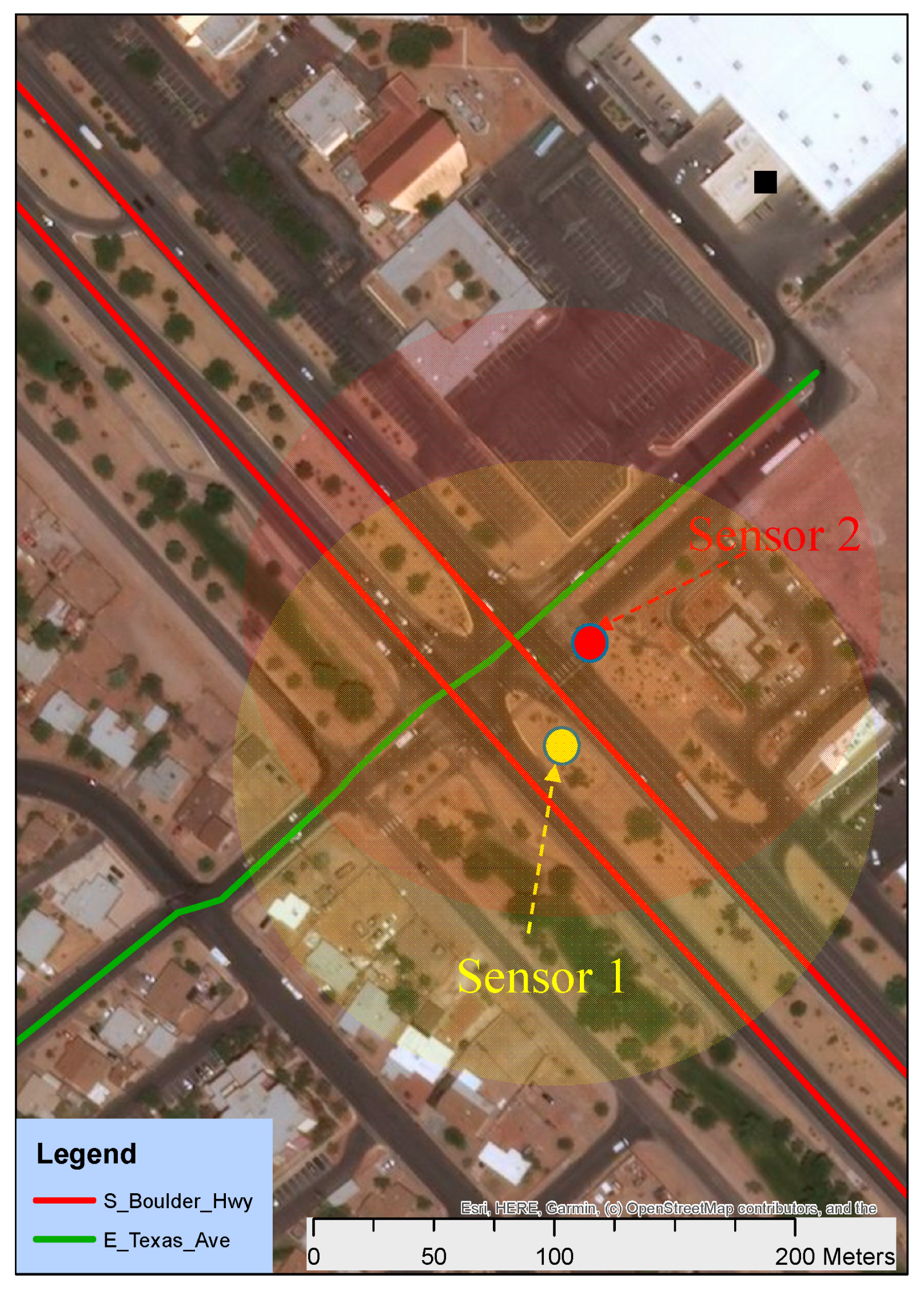
The developed procedure for integrating multiple roadside LiDAR sensor data was evaluated with the LiDAR data collected with two Velodyne VLP-16 LiDAR sensors at the intersection- S Boulder Hwy@ E Texas Ave, as shown in Figure 6. The data were collected to study the behaviors of vehicles/pedestrians/bicycles/skateboarders at the site. The two LiDAR datasets needed to be integrated before extracting the trajectories of the road users.
The VLP-16 LiDAR sensor is a cost-effective 3D LiDAR unit. The LiDAR sensor creates a 360° 3D point cloud with 16 laser beams. The unit inside rapidly spins to scan the surrounding environment with a detection range of 100 m (328 ft). The LiDAR has the rotation frequency in the range of 5–20 Hz. It can generate 600,000 3D points per second. The sensor’s low power consumption (~8w), lightweight (830g), compact footprint, dual return capability, and reasonable price make it ideal for roadside deployment for serving connected vehicles and other traffic engineering applications. Each VLP-16 reports the cloud points’ locations (x, y, and z) in a local coordinate system with the sensor at the origin. The rotation frequency was set as 10 Hz in the data collection. One frame from each LiDAR sensor dataset was extracted for the LiDAR data integration/registration.
For Sensor 1, the boundaries for the ground points extraction were defined as x: −35~35 m, y: −20~10 m, and z: −2~1 m. For Sensor 2, the boundaries for the ground points extraction were defined as x: −20~10 m, y: −35~35 m, and z: −3~2 m. The boundaries need to be selected with consideration of the sensor location, surrounding environment, and terrain. Two reference points at building corners were selected in this test.
3.1. Performance of GA Optimization
The computer was configured with Intel I7-3740QM CPU @ 2.70 GHz and 16 GB memory (RAM). Because of the distance of the LiDAR sensors and different surrounding environments of trees and obstacles, it is difficult to evaluate the results quantitatively, so this paper assessed the accuracy based on the visualization of the registered LiDAR data and checks points of the building surface and a parked vehicle. Figure 7 visualizes the integrated data of two LiDAR sensors with GA optimization. Figure 7a shows minor offsets in x-axis and y-axis of the building edges in the box. Figure 7b shows a mismatch in the z-axis of the LiDAR points of the building edges, as surrounded by the box.
3.2. Performance of HC Optimization
With the visualization tool, the initial parameters that were the input of HC were estimated. The transformation parameters were optimized by the HC method with the objective function. The computation time was 34 s. Figure 8 presents the registration results of HC.
The LiDAR data registration converted the Sensor 2 data into the Sensor 1 coordinate with a relatively accurate match. The boxes in Figure 8a highlight the exact matches of the building edges in 2D and the box in Figure 8b highlights the match of the building edges in 3D. It should be noted that there should be some offsets in z-axis, since the heights of the LiDARs were different.
Based on the testing with the GA method and the HC method, HC can provide more accurate registration of the two datasets. Although the GA method is a global optimization method, it can only give an estimation of the optimization solution. The GA method does not guarantee the minimum objective function to be found, and each run offered different parameters [40]. On the other hand, the HC algorithm is a local optimization algorithm, but it can give actual optimization results with the initial input estimated by the visualization tool. The integrated point clouds can generate the vehicle trajectories with higher accuracy. An example of the integrated vehicle trajectories can be found at https://youtu.be/s5MT1UrabeQ.
3.3. Comparison to ICP
The RGP method was also compared to the existing method—a revised ICP algorithm [35]. To evaluate the results of the two methods quantitatively, the LiDAR points were firstly mapped from the local coordinate system to the World Geodetic System-WGS-84. Figure 9 shows an example of integrated sensor data at one intersection in Reno. Here, the locations of the infrastructures (such as the corner of the buildings) in Google Earth were considered as the “ground truth” data.
The distance (D) between the LiDAR data and the corresponding infrastructure (such as the corner of the building) was manually checked by the authors. The data were collected at four sites: N McCarran @ Evans Ave, S Boulder Hwy @ E Texas Ave, I-80 @ Keystone Avenue, and I-80 @ N McCarran. For each site, an average D was calculated by randomly selecting 10 points. The results of the RGP and the revised ICP are summarized in Table 2. It is clearly shown that the RGP can generate a smaller error than the revised ICP at each site.
4. Discussion
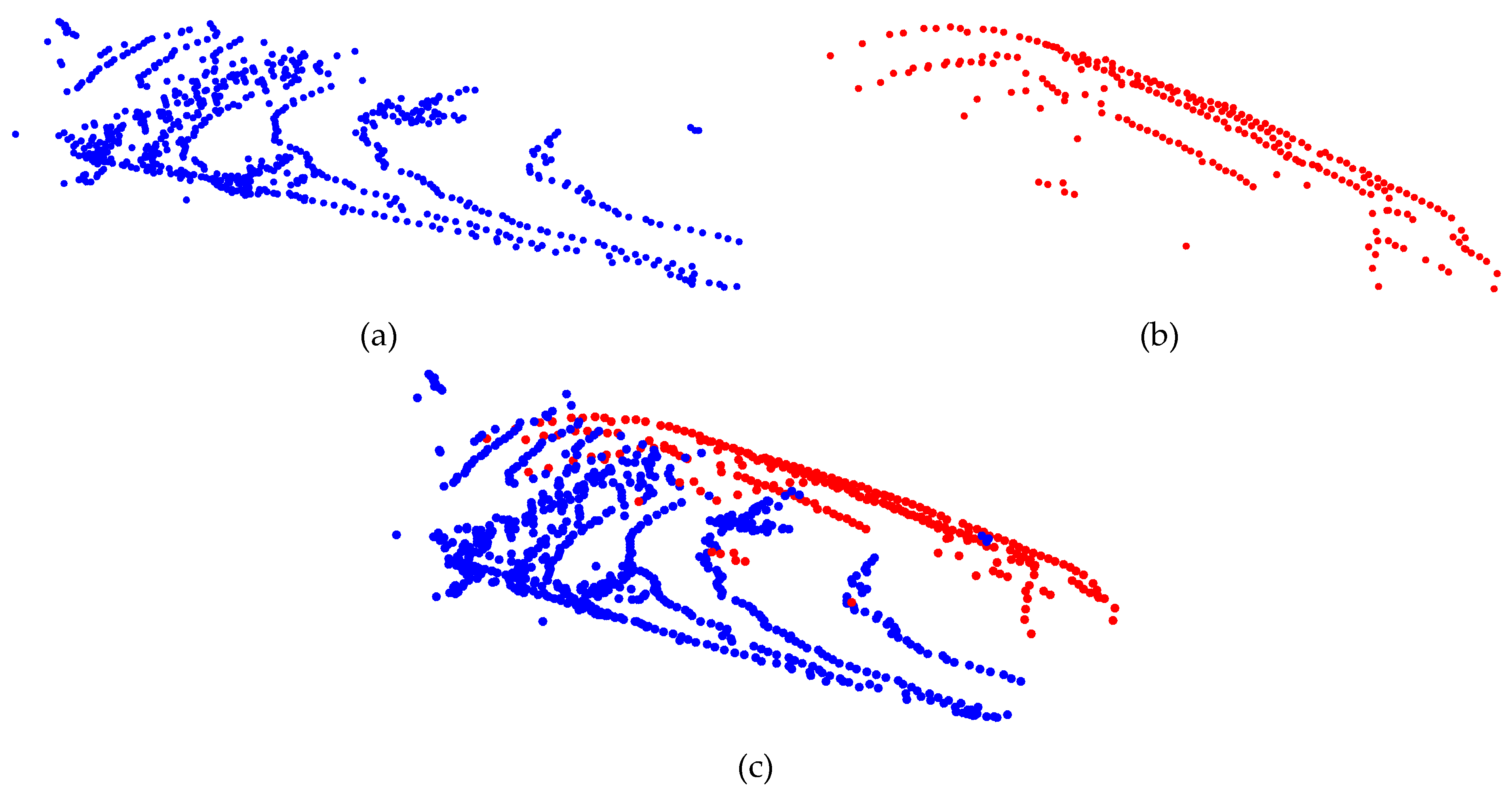
The advantages of LiDAR sensors and the recently reduced unit prices triggered the innovative application of LiDAR sensors at traffic infrastructures, which can uniquely offer high-resolution high-accuracy trajectory data of all traffic users [41,42,43,44]. The deployment of LiDAR sensors provides the data required by connected-vehicle systems and will reform different areas of traffic engineering and research. Integration of multiple roadside LiDAR sensors is significant to the roadside LiDAR application. The integrated point clouds can reduce the influence of occlusion issue (one object is blocked by another object) and improve the shape of road users in the LiDAR data. Figure 10 shows the vehicle shape before-and-after data integration using the proposed RGP method.
It is shown that the proposed RGP method can greatly improve the shape of road users. This paper only evaluates the integration results using two LiDAR sensors. In theory, the method can be used to integrate multiple LiDAR sensors. However, the authors did not validate it since the authors’ team only has two LiDAR sensors now. Another advantage of the proposed method is that the proposed RGP method can integrate the LiDAR data without knowing the GPS positions of the point clouds. Based on the statistical analysis, the proposed RGP method can integrate LiDAR points with a higher accuracy compared to the ICP. Future studies should compare the performance of the RGP method with other methods, such as the generalized-ICP (G-ICP). The future research will be to test the performance of the proposed method at more sites with more sensors. For LiDAR sensors with a long distance between them may not have enough overlaps of the ground surface points, portable LiDAR sensors will be considered as a bridging tool.
5. Conclusions
This article introduces a foundation work to register multiple LiDAR sensors deployed along roadsides into a uniform coordinate. As there are rare overlap points corresponding to reference features (points, lines, and planes) in the roadside LiDAR datasets, the existing methodologies cannot be used for the roadside LiDAR registration. An innovative procedure—RGP—was developed to use the ground surface LiDAR points in 3D space, and reference points in 2D space to generate the coordinate transformation that converts different LiDAR datasets into the same coordinate. The RGP can overcome the challenges caused by the offsets of laser beams between sensors and the low density of LiDAR sensors caused by the extended detection range.
Two optimization methods—the GA method (global optimization) and the HC algorithm (local optimization)—were considered for identifying the optimized transformation parameters for the RGP in this research. It was found that the GA method could not guarantee the minimized objective function. The HC algorithm accurately optimized the parameters with the initial input estimated by a visualization tool. Therefore, the HC algorithm was recommended for the parameters optimization for the RGP.
Author Contributions
Conceptualization, R.Y., H.X., and J.W.; methodology, B.L., R.Y., H.X., J.W., and C.Y.; validation, B.L., R.Y., H.X., J.W., R.S., and C.Y.; writing—original draft preparation, H.X. and J.W.; writing—review and editing, B.L., R.Y., H.X., J.W., R.S., and C.Y.
Funding
This research was supported in part by the Fundamental Research Funds for the Central Universities under Grant (NO.300102238614), in part by the Ministry of education of Humanities and Social Science project under grant (NO.18YJAZH120), in part by the Natural Science Foundation of China under Grant 61463026 and Grant 61463027, in part by Foundation of A Hundred Youth Talents Training Program of Lanzhou Jiaotong University.
Acknowledgments
The authors would like to gratefully acknowledge Zong Tian and Hongchao Liu who provided us the data support.
Conflicts of Interest
The authors declare no conflict of interest.
References
- Gupta, A.; Jha, R.K. A survey of 5G network: Architecture and emerging technologies. IEEE Access 2015, 3, 1206–1232. [Google Scholar] [CrossRef]
- Kenney, J.B. Dedicated short-range communications (DSRC) standards in the United States. Proc. IEEE 2011, 99, 1162–1182. [Google Scholar] [CrossRef]
- Biswas, S.; Tatchikou, R.; Dion, F. Vehicle-to-vehicle wireless communication protocols for enhancing highway traffic safety. IEEE Commun. Mag. 2006, 44, 74–82. [Google Scholar] [CrossRef]
- Wu, J.; Tian, Y.; Xu, H.; Yue, R.; Wang, A.; Song, X. Automatic ground points filtering of roadside LiDAR data using a channel-based filtering algorithm. Opt. Laser Technol. 2019, 115, 374–383. [Google Scholar] [CrossRef]
- Zhao, J.; Xu, H.; Liu, H.; Wu, J.; Zheng, Y.; Wu, D. Detection and tracking of pedestrians and vehicles using roadside LiDAR sensors. Transp. Res. Part C Emerg. Technol. 2019, 100, 68–87. [Google Scholar] [CrossRef]
- Wu, J.; Xu, H.; Zheng, J. Automatic Background Filtering and Lane Identification with Roadside LiDAR Data. In Proceedings of the IEEE 20th International Conference on Intelligent Transportation, Yokohama, Japan, 16–19 October 2017; pp. 1–6. [Google Scholar]
- Sun, Y.; Xu, H.; Wu, J.; Zheng, J.; Dietrich, K. 3-D Data Processing to Extract Vehicle Trajectories from Roadside LiDAR Data. Transp. Res. Rec. 2019, 2672, 14–22. [Google Scholar] [CrossRef]
- Wu, J. An Automatic Procedure for Vehicle Tracking with a Roadside LiDAR Sensor. ITE J. 2018, 88, 32–37. [Google Scholar]
- Zheng, Y.; Xu, H.; Tian, Z.; Wu, J. Design and Implementation of the DSRC Bluetooth Communication and Mobile Application with LiDAR Sensor. In Proceedings of the 97th Transportation Research Board Annual Meeting, Washington, DC, USA, 7–11 January 2018. [Google Scholar]
- Zhao, J.; Xu, H.; Wu, D.; Liu, H. An Artificial Neural Network to Identify Pedestrians and Vehicles from Roadside 360-Degree LiDAR Data. In Proceedings of the 97th Transportation Research Board Annual Meeting, Washington, DC, USA, 7–11 January 2018. [Google Scholar]
- Lv, B.; Xu, H.; Wu, J.; Tian, Y.; Tian, S.; Feng, S. Revolution and rotation-based method for roadside LiDAR data integration. Opt. Laser Technol. 2019, 119, 105571. [Google Scholar] [CrossRef]
- Gebre, B.A.; Men, H.; Pochiraju, K. Remotely operated and autonomous mapping system (ROAMS). In Proceedings of the IEEE International Conference on Technologies for Practical Robot Applications, Woburn, MA, USA, 9–10 November 2009; pp. 173–178. [Google Scholar]
- Liu, S.; Tong, X.; Chen, J.; Liu, X.; Sun, W.; Xie, H.; Chen, P.; Jin, Y.; Ye, Z. A linear feature-based approach for the registration of unmanned aerial vehicle remotely-sensed images and airborne LiDAR data. Remote Sens. 2016, 8, 82. [Google Scholar] [CrossRef]
- Schwarz, B. LIDAR: Mapping the world in 3D. Nat. Photonics 2010, 4, 429–430. [Google Scholar] [CrossRef]
- Chen, J.; Wu, X.; Wang, M.Y.; Li, X. 3D shape modeling using a self-developed hand-held 3D laser scanner and an efficient HT-ICP point cloud registration algorithm. Opt. Laser Technol. 2013, 45, 414–423. [Google Scholar] [CrossRef]
- Jaw, J.; Chuang, T. Feature-based registration of terrestrial lidar point clouds. Int. Arch. Photogramm. Remote Sens. Spat. Inf. Sci. 2008, 37, 303–308. [Google Scholar]
- Besl, P.J.; McKay, N.D. Method for registration of 3-D shapes. In Sensor Fusion IV: Control Paradigms and Data Structures; International Society for Optics and Photonics: Bellingham, DC, USA, 1992; Volume 1611, pp. 586–607. [Google Scholar]
- Wu, J.; Xu, H.; Liu, W. Points Registration for Roadside LiDAR Sensors. Transp. Res. Rec. 2019, in press. [Google Scholar] [CrossRef]
- Turk, G.; Levoy, M. Zippered polygon meshes from range images. In Proceedings of the 21st Annual Conference on Computer Graphics and Interactive Techniques, Orlando, FL, USA, 24–29 July 1994; pp. 311–318. [Google Scholar]
- Masuda, T.; Sakaue, K.; Yokoya, N. Registration and integration of multiple range images for 3-D model construction. In Proceedings of the 13th International Conference on Pattern Recognition, Vienna, Austria, 25–19 August 1996; Volume 1, pp. 879–883. [Google Scholar]
- Godin, G.; Rioux, M.; Baribeau, R. Three-dimensional registration using range and intensity information. In Videometrics III; SPIE: Boston, MA, USA, 1994; Volume 2350, pp. 279–291. [Google Scholar]
- Jost, T.; Hugli, H. A multi-resolution scheme ICP algorithm for fast shape registration. In Proceedings of the First International Symposium on 3D Data Processing Visualization and Transmission, Padova, Italy, 19–21 June 2002; pp. 540–543. [Google Scholar]
- Gelfand, N. Feature Analysis and Registration of Scanned Surfaces; Stanford University: Stanford, CA, USA, 2006. [Google Scholar]
- Stamos, I.; Allen, P.K. Geometry and texture recovery of scenes of large scale. Comput. Vis. Image Underst. 2002, 88, 94–118. [Google Scholar] [CrossRef]
- Stamos, I.; Leordeanu, M. Automated feature-based range registration of urban scenes of large scale. In Proceedings of the IEEE Computer Society Conference on Computer Vision and Pattern Recognition, Madison, WI, USA, 16–22 June 2003; pp. 2–7. [Google Scholar]
- Habib, A.; Ghanma, M.; Morgan, M.; Al-Ruzouq, R. Photogrammetric and LiDAR data registration using linear features. Photogramm. Eng. Remote Sens. 2005, 71, 699–707. [Google Scholar] [CrossRef]
- Akca, D. Full Automatic Registration of Laser Scanner Points Clouds; ETH Zurich: Zurich, Switzerland, 2003. [Google Scholar]
- Rabbani, T.; Dijkman, S.; van den Heuvel, F.; Vosselman, G. An integrated approach for modelling and global registration of point clouds. ISPRS J. Photogramm. Remote Sens. 2007, 61, 355–370. [Google Scholar] [CrossRef]
- Von Hansen, W. Registration of Agia Sanmarina LIDAR data using surface elements. In Proceedings of the ISPRS Workshop on Laser Scanning; ISPRS: Espoo, Finland, 2007; pp. 93–97. [Google Scholar]
- Bodensteiner, C.; Arens, M. Real-time 2D video/3D LiDAR registration. In Proceedings of the 21st International Conference on Pattern Recognition (ICPR2012), Tsukuba, Japan, 11–15 November 2012; pp. 2206–2209. [Google Scholar]
- Giering, M.; Venugopalan, V.; Reddy, K. Multi-modal sensor registration for vehicle perception via deep neural networks. In Proceedings of the IEEE High Performance Extreme Computing Conference (HPEC), Waltham, MA, USA, 15–17 September 2015; pp. 1–6. [Google Scholar]
- Cho, H.; Seo, Y.W.; Kumar, B.V.; Rajkumar, R.R. A multi-sensor fusion system for moving object detection and tracking in urban driving environments. In Proceedings of the IEEE International Conference on Robotics and Automation (ICRA), Hong Kong, China, 31 May–7 June 2014; pp. 1836–1843. [Google Scholar]
- Mertz, C.; Navarro-Serment, L.E.; MacLachlan, R.; Rybski, P.; Steinfeld, A.; Suppé, A.; Urmson, C.; Vandapel, N.; Hebert, M.; Thorpe, C.; et al. Moving object detection with laser scanners. J. Field Robot. 2013, 30, 17–43. [Google Scholar] [CrossRef]
- Wu, J.; Xu, H.; Lv, B.; Yue, R.; Li, Y. Automatic Ground Points Identification Method for Roadside LiDAR Data. Transp. Res. Rec. 2019, 2673. [Google Scholar] [CrossRef]
- Wu, J.; Xu, H.; Zheng, Y.; Tian, Z. A novel method of vehicle-pedestrian near-crash identification with roadside LiDAR data. Accid. Anal. Prev. 2018, 121, 238–249. [Google Scholar] [CrossRef]
- Golberg, D.E. Genetic Algorithms in Search, Optimization, and Machine Learning; Addion Wesley: Reading, MA, USA, 1989; p. 36. [Google Scholar]
- Russell, S.J.; Norvig, P. Artificial Intelligence: A Modern Approach; Pearson Education Limited: Kuala Lumpur, Malaysia, 2016. [Google Scholar]
- Weise, T. Global Optimization Algorithms-Theory and Application. Available online: http://www.it-weise.de/projects/book.pdf (accessed on 7 April 2019).
- Genetic Algorithm and Direct Search Toolbox™ 2 User’s Guide. Available online: https://laboratoriomatematicas.uniandes.edu.co/metodos/contenido/contenido/ag.pdf (accessed on 7 May 2019).
- Houck, C.R.; Joines, J.; Kay, M.G. A genetic algorithm for function optimization: A Matlab implementation. Ncsu-ie tr 1995, 95, 1–10. [Google Scholar]
- Zheng, J.; Yang, S.; Wang, X.; Xia, X.; Xiao, Y.; Li, T. A Decision Tree based Road Recognition Approach using Roadside Fixed 3D LiDAR Sensors. IEEE Access 2019, 7, 53878–53890. [Google Scholar] [CrossRef]
- Cui, Y.; Xu, H.; Wu, J.; Sun, Y.; Zhao, J. Automatic Vehicle Tracking with Roadside LiDAR Data for the Connected-Vehicles System. IEEE Intell. Syst. 2019, in press. [Google Scholar] [CrossRef]
- Chen, J.; Xu, H.; Wu, J.; Yue, R.; Yuan, C.; Wang, L. Deer Crossing Road Detection with Roadside LiDAR Sensor. IEEE Access 2019, 7, 65944–65954. [Google Scholar] [CrossRef]
- Wu, J.; Xu, H.; Sun, Y.; Zheng, J.; Yue, R. Automatic background filtering method for roadside LiDAR data. Transp. Res. Rec. 2018, 2672, 106–114. [Google Scholar] [CrossRef]
Figure 1.
Cloud points from roadside cost-efficient LiDAR sensor. (a) Relative high-density LiDAR cloud points (64 beams). (b) Relative low-density LiDAR cloud points (16 beams).
Figure 1.
Cloud points from roadside cost-efficient LiDAR sensor. (a) Relative high-density LiDAR cloud points (64 beams). (b) Relative low-density LiDAR cloud points (16 beams).
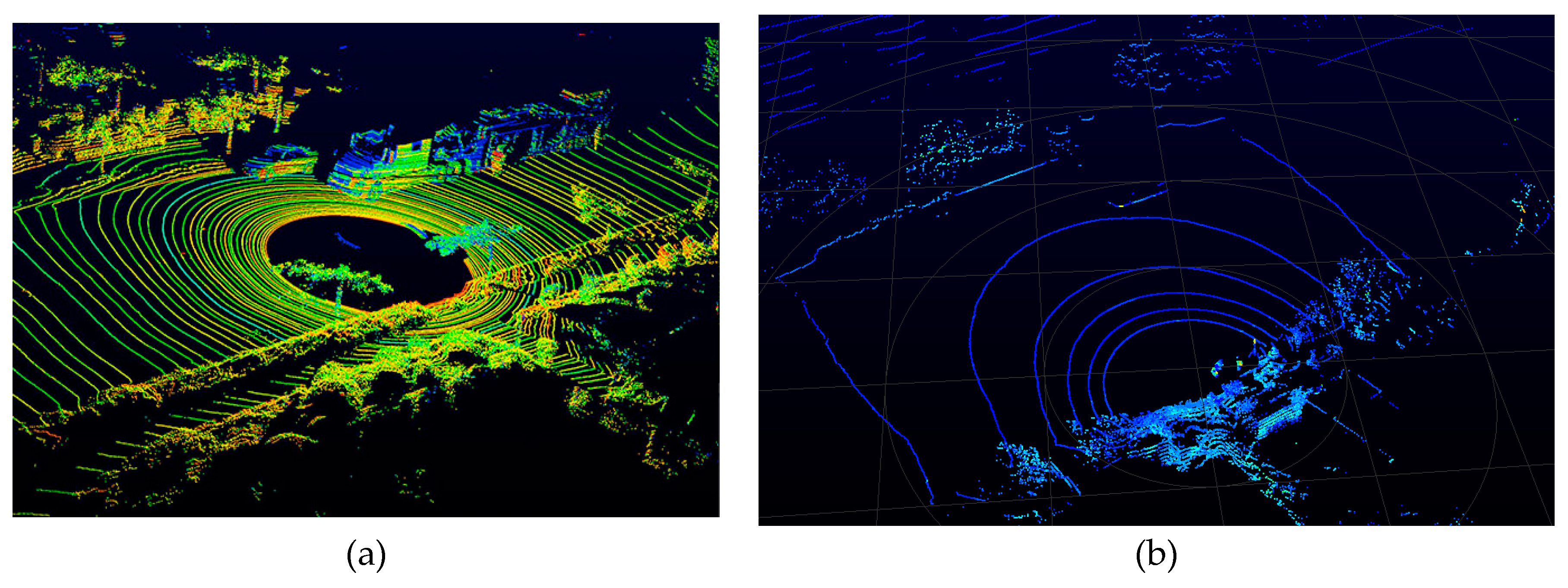
Figure 2.
Example of z-axis offset between two roadside LiDAR datasets.

Figure 3.
Example of ground points overlaps of two LiDAR datasets.
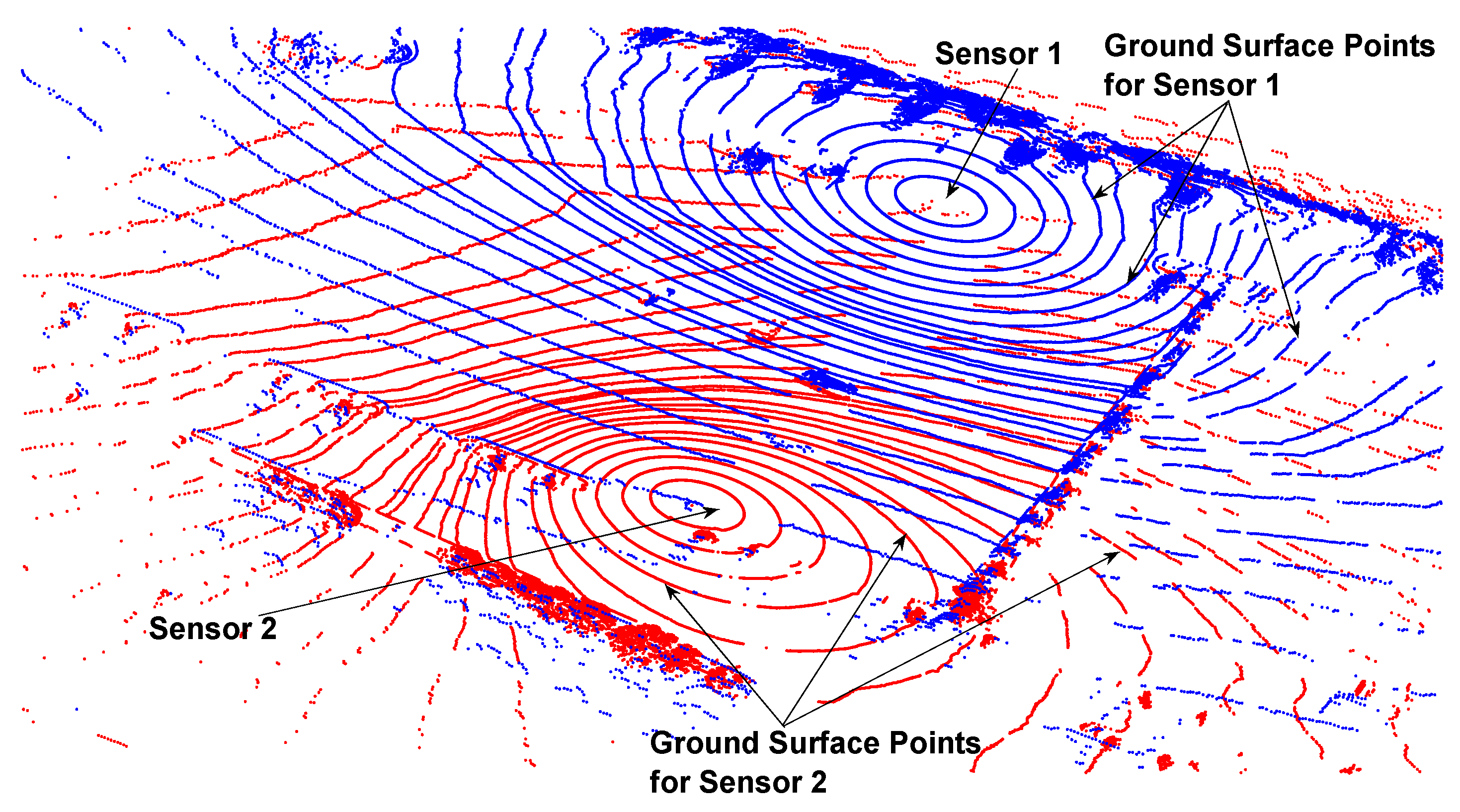
Figure 4.
Genetic algorithm (GA) optimization.

Figure 5.
General procedure of hill climbing (HC) algorithm.

Figure 6.
Field site selected for evaluation.

Figure 7.
LiDAR data registration with the GA. (a) XY Plane. (b) Z-axis.

Figure 8.
LiDAR data registration with the HC. (a) XY Plane. (b) Z-axis.
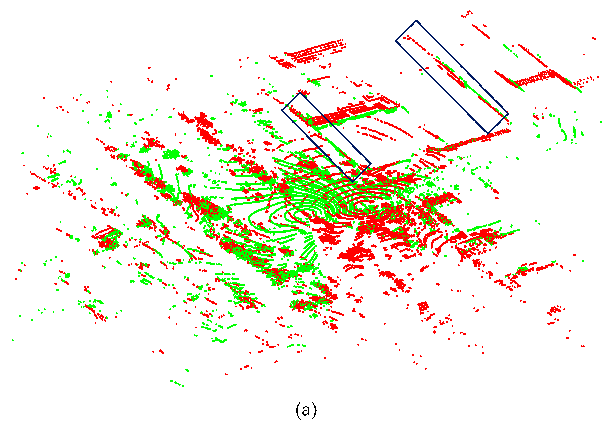

Figure 9.
LiDAR data mapped into Google Earth.

Figure 10.
Before-and-after data integration. (a) Vehicle in Sensor A. (b) Vehicle in Sensor B. (c) Integrated vehicle.
Figure 10.
Before-and-after data integration. (a) Vehicle in Sensor A. (b) Vehicle in Sensor B. (c) Integrated vehicle.


Table 1.
Parameters in GA.
| Parameters | Setting | Note |
|---|---|---|
| Population size | 150 | Number of individuals in each generation |
| Creation function | Uniform function | Random initial population |
| Initial range | [−50, −50, −50, −180, −180, −180; 50, 50, 50, 180, 180, 180] | The offsets along axis are −50 m to 50 m and the rotation angles around axis are −180 degrees to 180 degrees |
| Scaling function | Rank scaling | The raw scores were scaled based on the rank of the individuals |
| Selection function | Stochastic uniform | Parents selection for the next generation |
| Elite count | 0.05 * population size | Number of individuals that are guaranteed to survive to the next generation |
| Crossover fraction | 0.8 (default value) | Fraction of the next generation |
| Crossover function | Scattered crossover | The function that performs the crossover |
| Mutation function | Adaptive feasible | Provides genetic diversity and enables the genetic algorithm to search a broader space |
| Nonlinear constraint | The distance from the converted second sensor coordinate to the coordinate of the first sensor is less than 100 m | Search boundary |
| Stopping criteria | Max generations = 150 Max stall generations = 100 Function tolerance= 1 × 10⁻¹⁰ | Termination thresholds |
Table 2.
Performance evaluation.
| Site | D (meters) | |
|---|---|---|
| RGP | Revised ICP | |
| N McCarran @ Evans Ave | 0.25 | 1.1 |
| S Boulder Hwy @ E Texas Ave | 0.31 | 1.5 |
| I-80 @ Keystone Avenue | 0.24 | 0.9 |
| I-80 @ N McCarran | 0.13 | 0.7 |
© 2019 by the authors. Licensee MDPI, Basel, Switzerland. This article is an open access article distributed under the terms and conditions of the Creative Commons Attribution (CC BY) license (http://creativecommons.org/licenses/by/4.0/).
Share and Cite
MDPI and ACS Style
Yue, R.; Xu, H.; Wu, J.; Sun, R.; Yuan, C. Data Registration with Ground Points for Roadside LiDAR Sensors. Remote Sens. 2019, 11, 1354. https://doi.org/10.3390/rs11111354
AMA Style
Yue R, Xu H, Wu J, Sun R, Yuan C. Data Registration with Ground Points for Roadside LiDAR Sensors. Remote Sensing. 2019; 11(11):1354. https://doi.org/10.3390/rs11111354
Chicago/Turabian StyleYue, Rui, Hao Xu, Jianqing Wu, Renjuan Sun, and Changwei Yuan. 2019. "Data Registration with Ground Points for Roadside LiDAR Sensors" Remote Sensing 11, no. 11: 1354. https://doi.org/10.3390/rs11111354
Note that from the first issue of 2016, this journal uses article numbers instead of page numbers. See further details here.