Parameterization of Urban Sensible Heat Flux from Remotely Sensed Surface Temperature: Effects of Surface Structure

 and
and
Abstract
:1. Introduction
2. Methodology and Data
2.1. TUF-3D
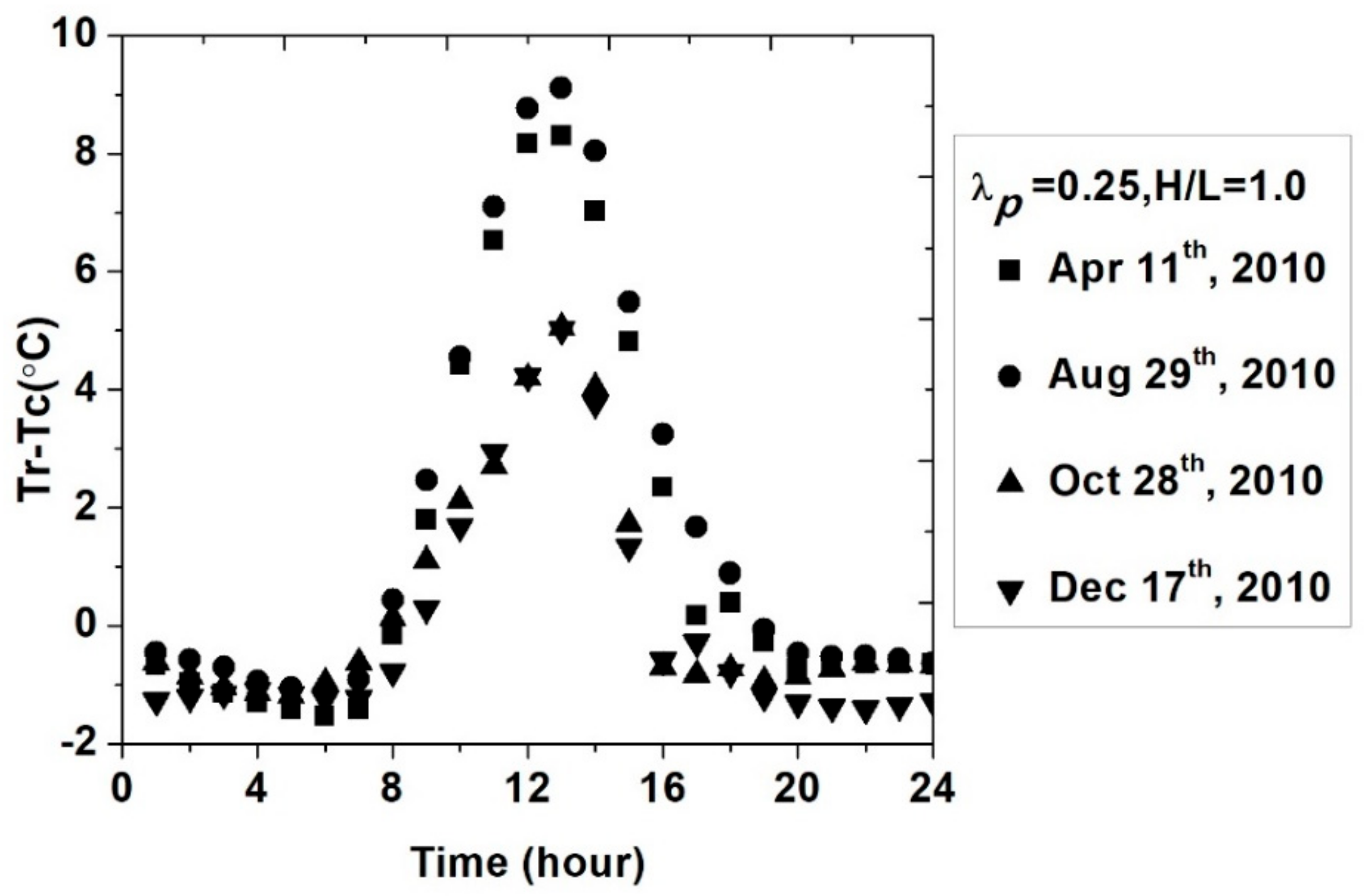
2.2. Complete versus Radiometric Urban Surface Temperature
2.3. Parameterization of Sensible Heat Flux
2.4. Parameterization of Resistance to Heat Transfer
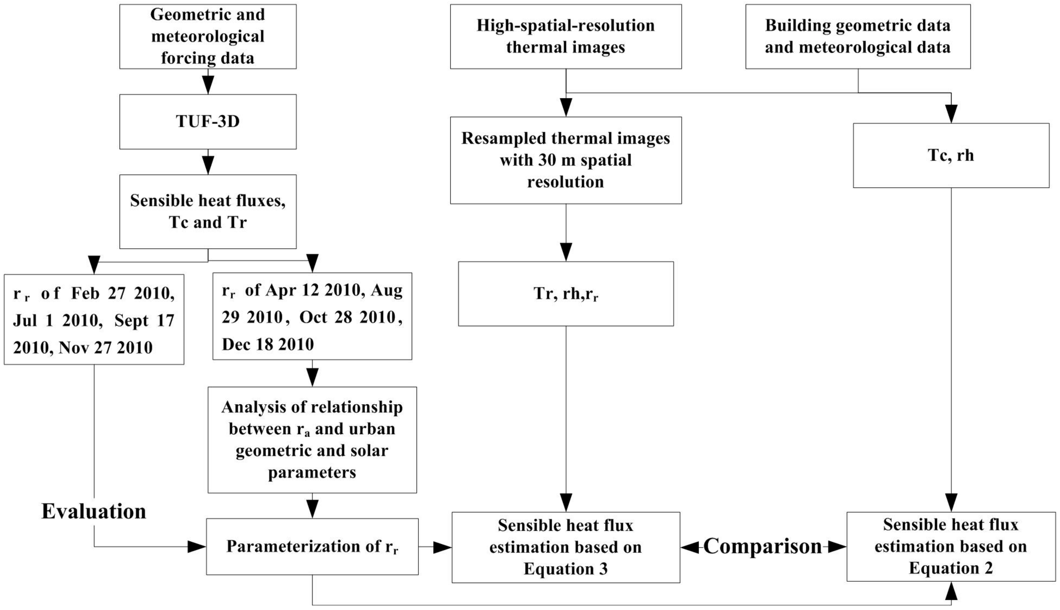
2.5. Experimental Design
2.6. Evaluation of the Parameterizations
3. Results
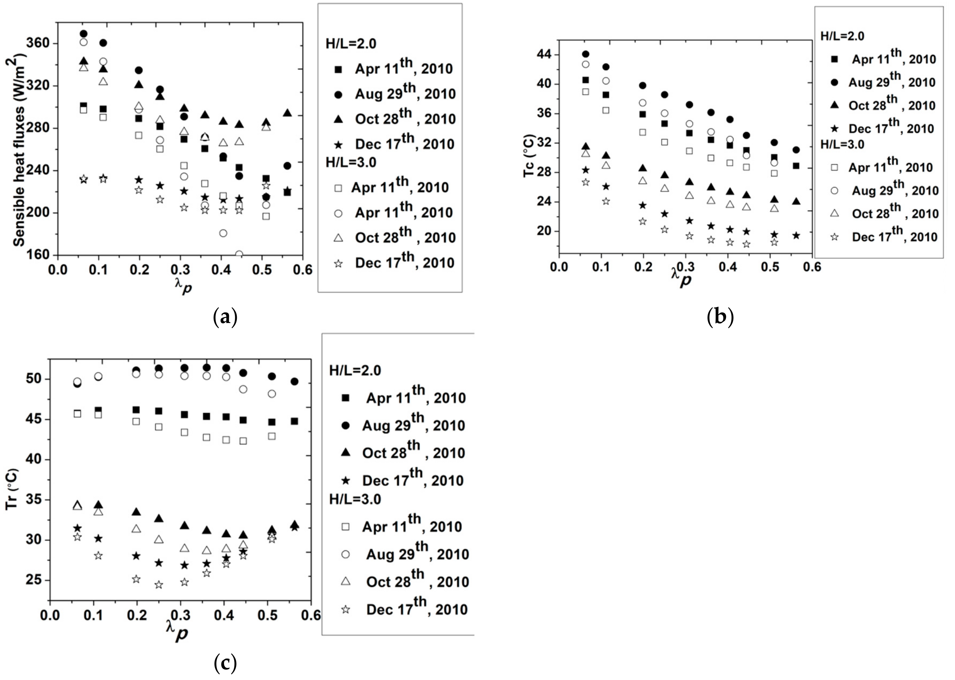
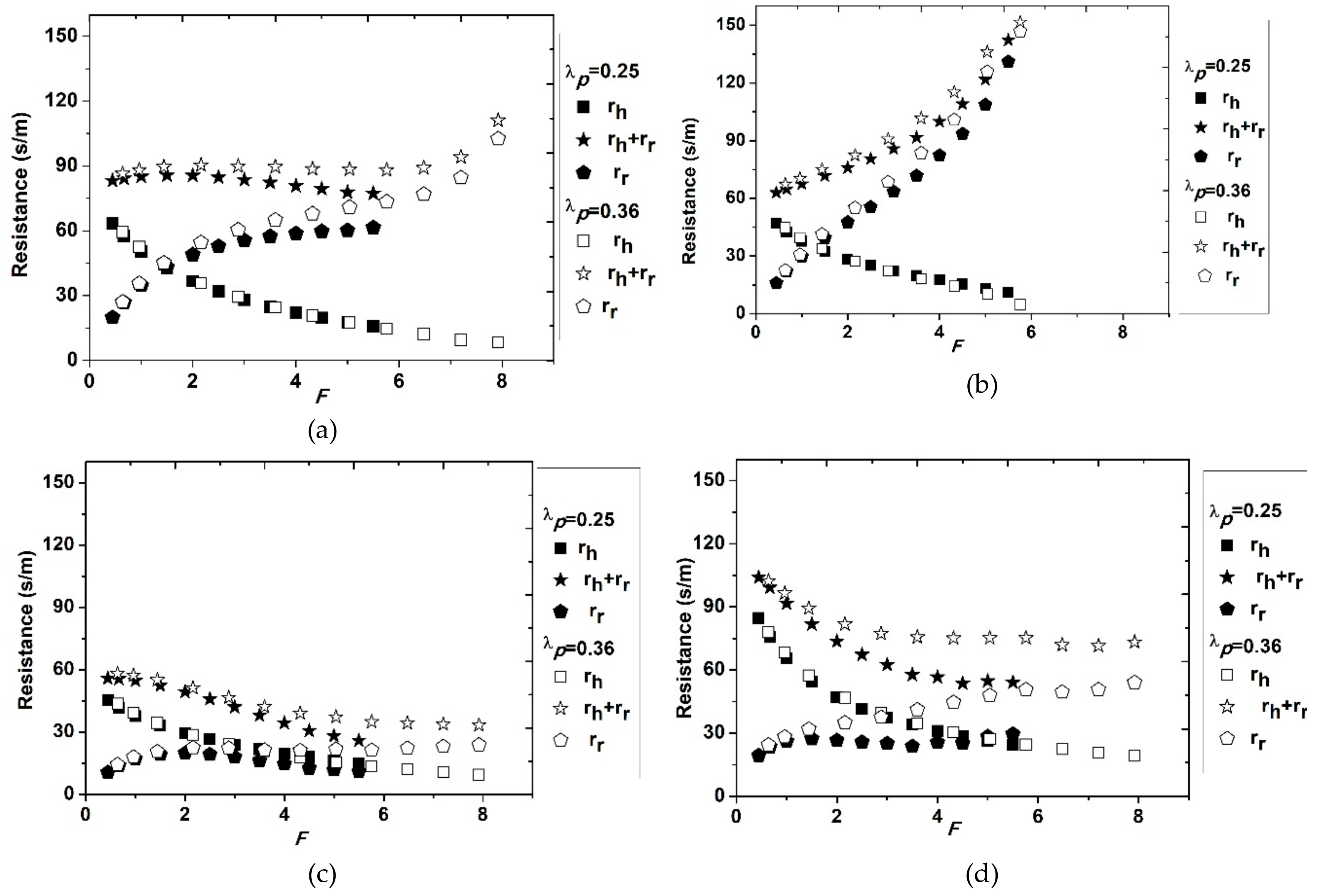
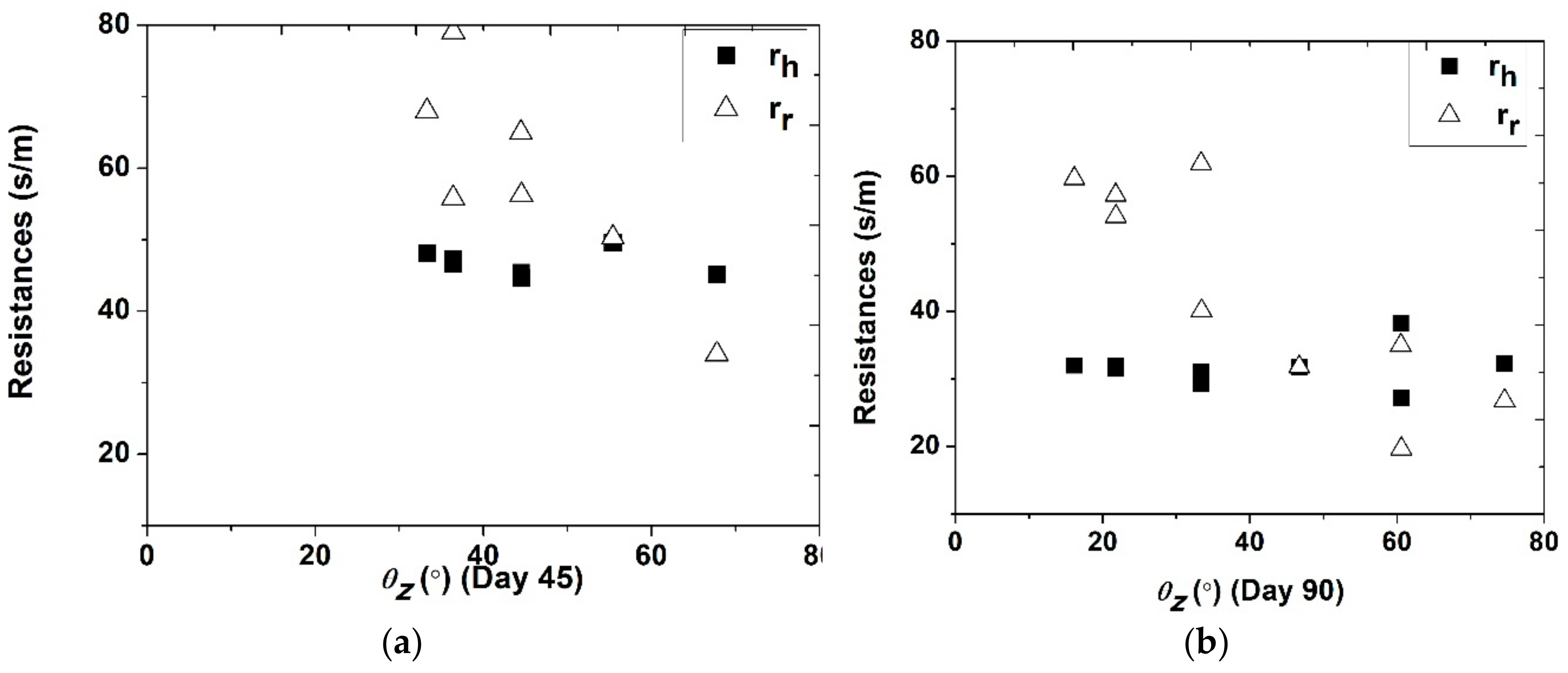
3.1. Sensitivity of and to Urban Geometry and Meteorological Forcing
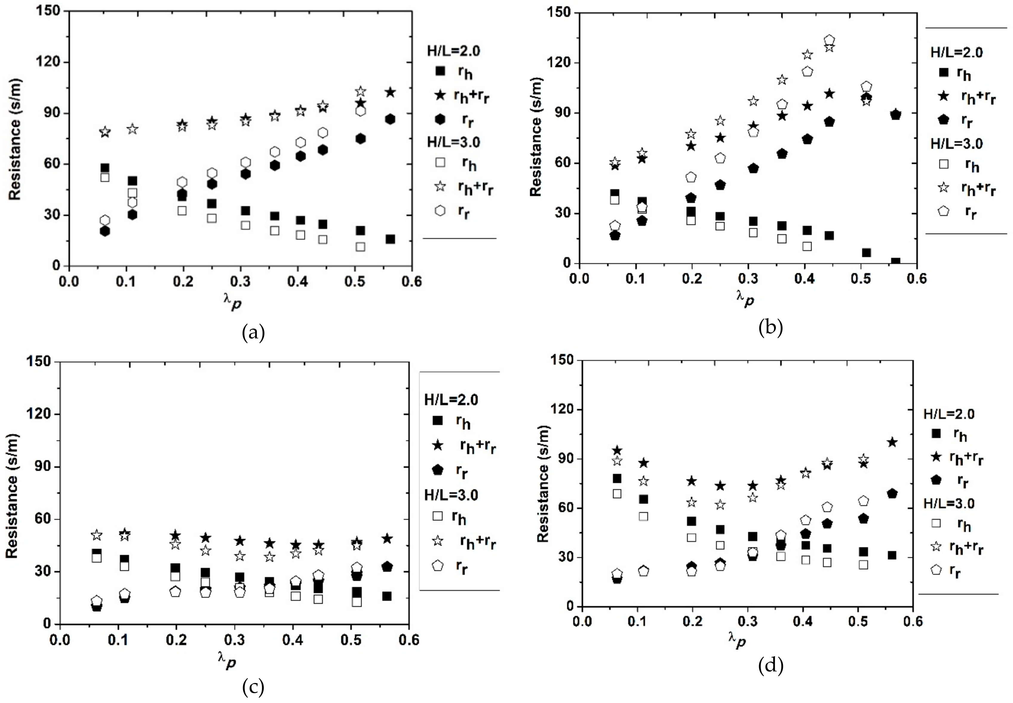
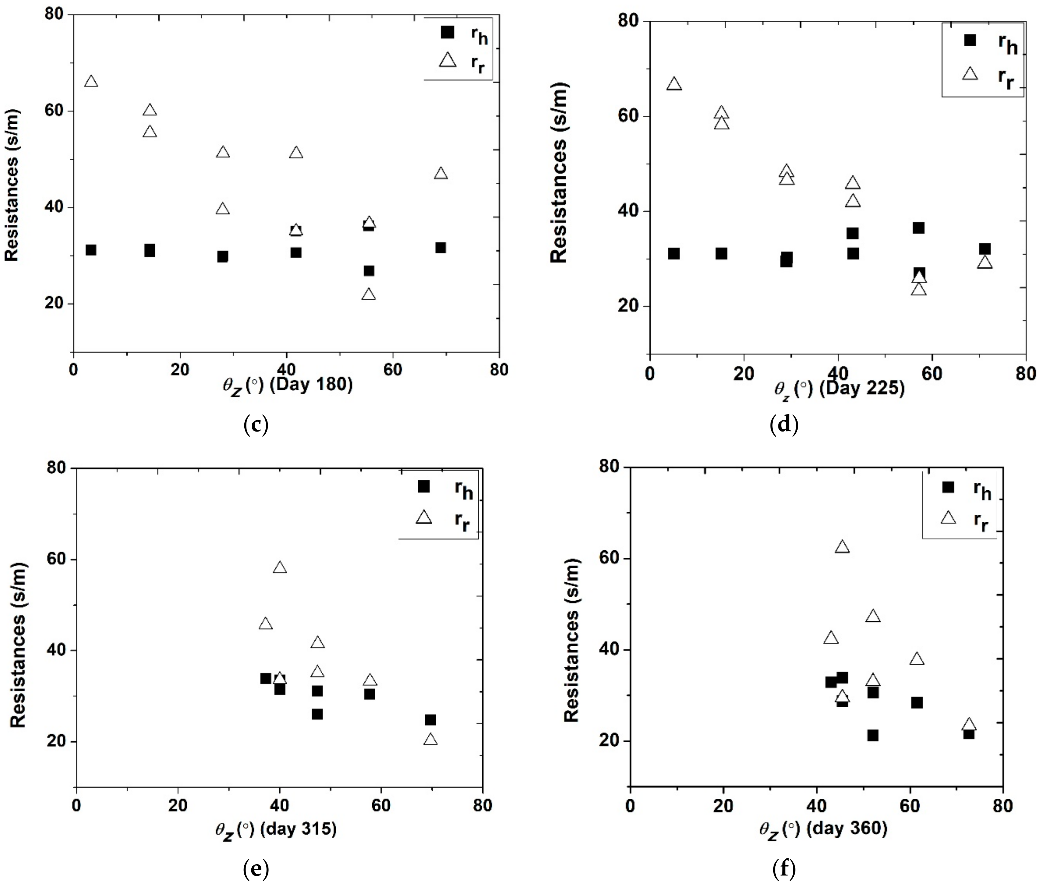
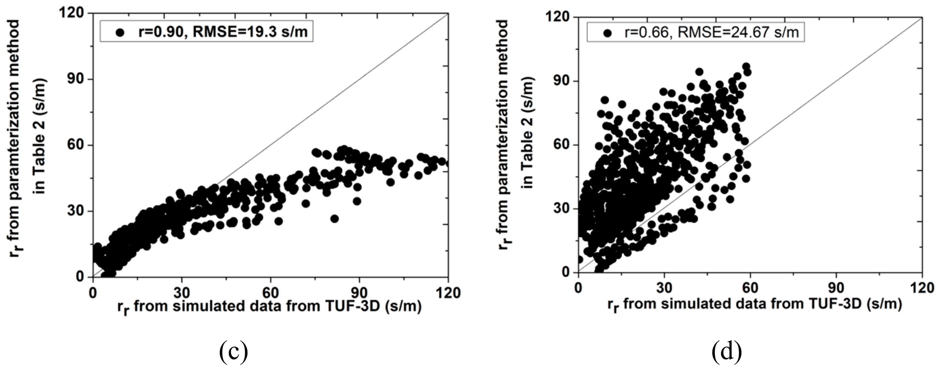
3.2. Parameterization of rr
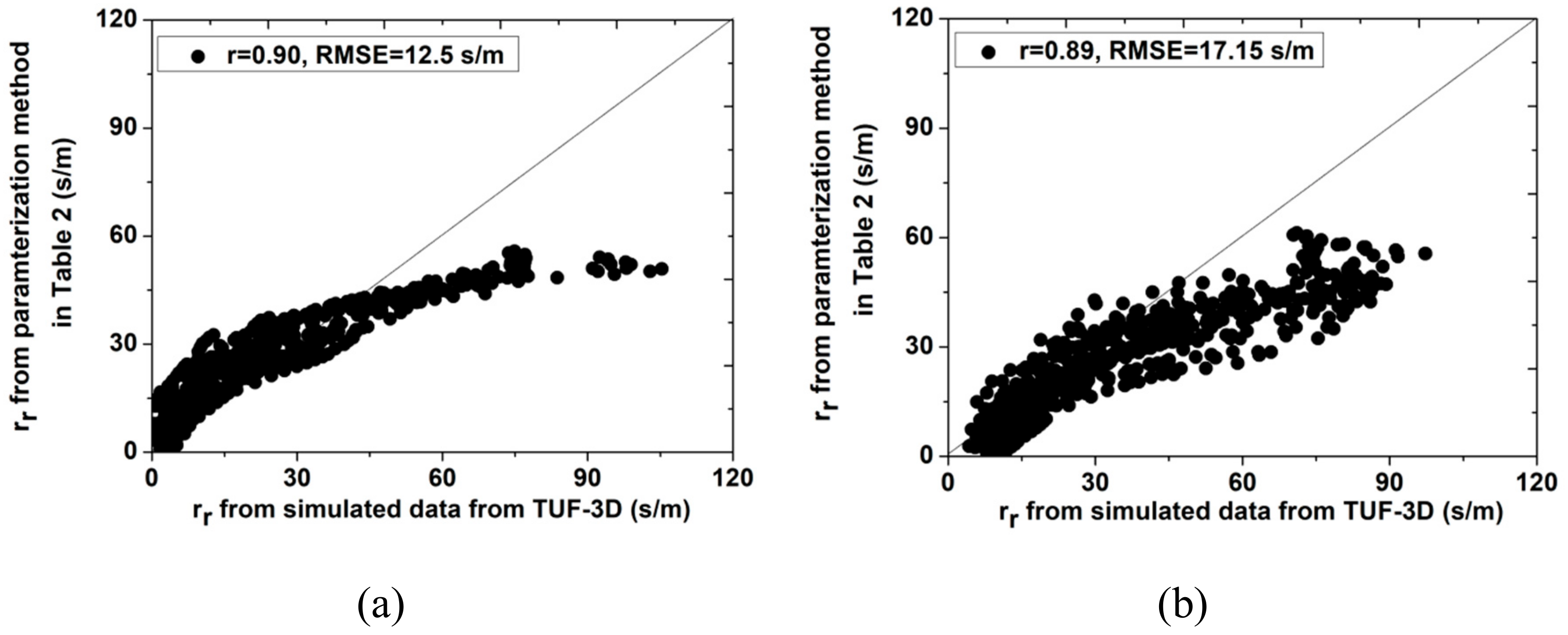
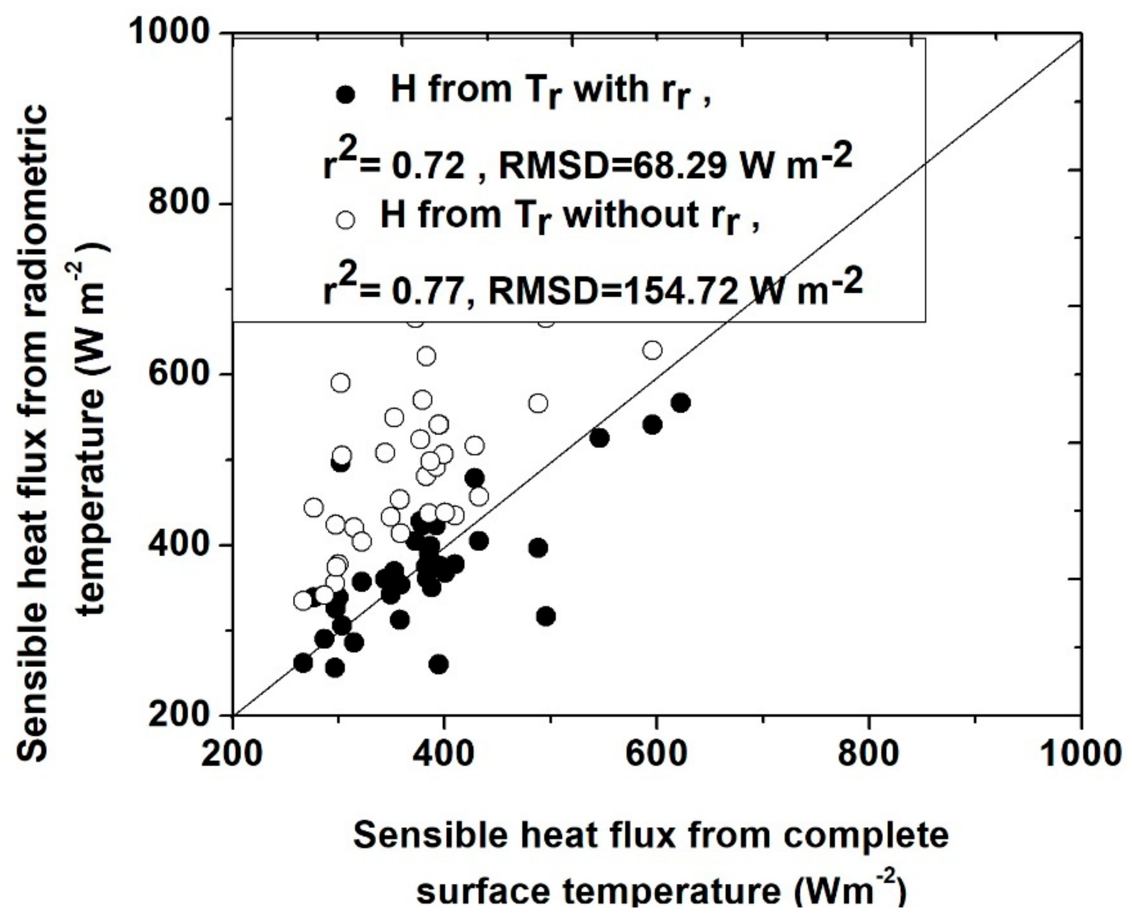
3.3. Evaluation of the Parameterization of
4. Discussion
5. Summary and Conclusions
Author Contributions
Funding
Acknowledgments
Conflicts of Interest
Appendix A

| 11 April 2010 | 29 August 2010 | 28 October 2010 | 17 December 2010 | |
|---|---|---|---|---|
| H/L = 2 | = −78.00 * + 58.68, r = 0.99 | = −75.27 * + 47.16, r = 0.98 | = −47.93 * + 42.17, r = 0.99 | = −84.10 * + 73.53, r = 0.95 |
| = 121.02 * + 16.179, r = 0.99 | = 163.89 * + 7.2, r = 0.97 | = 37.35 * + 9.48, r = 0.97 | = 99.54 * + 6.11, r = 0.96 | |
| H/L = 3 | = −86.01 * + 52.67, r = 0.98 | = −100.17 * + 46.05, r = 0.97 | = −56.39 * + 39.28, r = 0.99 | = −101.49 * + 67.47, r = 0.99 |
| = 132.86 * + 20.86, r = 0.99 | = 237.41 * + 7.72, r = 0.95 | = 36.11 * + 10.49, r = 0.92 | = 110.68 * + 5.40, r = 0.94 |
| 11 April 2010 | 29 August 2010 | 28 October 2010 | 17 December 2010 | |
|---|---|---|---|---|
| = 0.25 | = −19.45 * + 49.39, r = 0.99 | = −14.2 * + 37.13, r = 0.99 | = −12.27 * + 36.96, r = 0.99 | = −24.37 * + 64.90, r = 0.99 |
| = 17.02 * + 35.04, r = 0.99 | = 39.79 * + 32.40, r = 0.92 | = 4.25 * + 15.71, r = 0.88(aspect ratio < 3) | = 2.14 * + 23.86, r = 0.67 | |
| = 0.36 | = −20.83 * + 51.31, r = 0.99 | = −17.48 * + 37.13, r = 0.99 | = −14.09 * + 38.67, r = 0.99 | = −23.68 * + 66.20, r = 0.99 |
| = 24.57 * + 35.59, r = 0.96 | = 52.36 * + 29.56, r= 0.94 | = 2.62 * + 18.06, r = 0.85 | = 11.74 * + 27.88, r = 0.98 |
References
- Oke, T.; Cleugh, H.; Grimmond, C.; Schmid, H.; Roth, M. Evaluation of spatially-averaged fluxes of heat, mass and momentum in the urban boundary layer. Weather Clim. 1989, 9, 14–21. [Google Scholar] [CrossRef]
- Shahmohamadi, P.; Che-Ani, A.I.; Ramly, A.; Maulud, K.N.A.; Mohd-Nor, M.F.I. Reducing urban heat island effects: A systematic review to achieve energy consumption balance. Int. J. Phys. Sci. 2010, 5, 626–636. [Google Scholar]
- Kuang, W.; Dou, Y.; Zhang, C.; Chi, W.; Liu, A.; Liu, Y.; Liu, J. Quantifying the heat flux regulation of metropolitan land use/land cover components by coupling remote sensing modeling with in situ measurement. J. Geophys. Res. Atmos. 2015, 120, 113–130. [Google Scholar] [CrossRef]
- Oke, T.R. The energetic basis of the urban heat island. Q. J. R. Meteorol. Soc. 1982, 108, 1–24. [Google Scholar] [CrossRef]
- Nazarian, N.; Kleissl, J. CFD simulation of an idealized urban environment: Thermal effects of geometrical characteristics and surface materials. Urban Clim. 2015, 12, 141–159. [Google Scholar] [CrossRef]
- Krayenhoff, E.S.; Santiago, J.L.; Martilli, A.; Christen, A.; Oke, T.R. Parametrization of Drag and Turbulence for Urban Neighbourhoods with Trees. Bound. Layer Meteorol. 2015, 1–33. [Google Scholar] [CrossRef]
- Nazarian, N.; Martilli, A.; Norford, L.; Kleissl, J. Impacts of Realistic Urban Heating. Part II: Air Quality and City Breathability. Bound. Layer Meteorol. 2018. [Google Scholar] [CrossRef]
- Masson, V. A physically-based scheme for the urban energy budget in atmospheric models. Bound. Layer Meteorol. 2000, 94, 357–397. [Google Scholar] [CrossRef]
- Kusaka, H.; Kondo, H.; Kikegawa, Y.; Kimura, F. A simple single-layer urban canopy model for atmospheric models: Comparison with multi-layer and slab models. Bound. Layer Meteorol. 2001, 101, 329–358. [Google Scholar] [CrossRef]
- Martilli, A.; Clappier, A.; Rotach, M. An Urban Surface Exchange Parameterisation for Mesoscale Models. Bound. Layer Meteorol. 2002, 104, 261–304. [Google Scholar] [CrossRef]
- Voogt, J.A.; Grimmond, C. Modeling surface sensible heat flux using surface radiative temperatures in a simple urban area. J. Appl. Meteorol. 2000, 39, 1679–1699. [Google Scholar] [CrossRef]
- Xu, W.; Wooster, M.; Grimmond, C. Modelling of urban sensible heat flux at multiple spatial scales: A demonstration using airborne hyperspectral imagery of Shanghai and a temperature–emissivity separation approach. Remote Sens. Environ. 2008, 112, 3493–3510. [Google Scholar] [CrossRef]
- Kanda, M.; Kanega, M.; Kawai, T.; Moriwaki, R.; Sugawara, H. Roughness lengths for momentum and heat derived from outdoor urban scale models. J. Appl. Meteorol. Climatol. 2007, 46, 1067–1079. [Google Scholar] [CrossRef]
- Kastendeuch, P.P.; Najjar, G. Simulation and validation of radiative transfers in urbanised areas. Sol. Energy 2009, 83, 333–341. [Google Scholar] [CrossRef]
- Krayenhoff, E.S. A Multi-Layer Urban Canopy Model for Neighbourhoods with Trees. Ph.D. Thesis, University of British Columbia, Vancouver, BC, Canada, 2014. [Google Scholar]
- Nazarian, N.; Martilli, A.; Kleissl, J. Impacts of Realistic Urban Heating, Part I: Spatial Variability of Mean Flow, Turbulent Exchange and Pollutant Dispersion. Bound. Layer Meteorol. 2018, 166, 367–393. [Google Scholar] [CrossRef]
- Stewart, J.B.; Kustas, W.P.; Humes, K.S.; Nichols, W.D.; Moran, M.S.; De Bruin, H. Sensible heat flux-radiometric surface temperature relationship for eight semiarid areas. J. Appl. Meteorol. 1994, 33, 1110–1117. [Google Scholar] [CrossRef]
- Wang, L.; Li, D.; Gao, Z.; Sun, T.; Guo, X.; Bou-Zeid, E. Turbulent Transport of Momentum and Scalars Above an Urban Canopy. Bound. Layer Meteorol. 2014, 150, 485–511. [Google Scholar] [CrossRef]
- Kanda, M.; Moriwaki, R.; Kasamatsu, F. Spatial Variability of Both Turbulent Fluxes and Temperature Profiles in an Urban Roughness Layer. Bound. Layer Meteorol. 2006, 121, 339–350. [Google Scholar] [CrossRef]
- Kato, S.; Yamaguchi, Y. Estimation of storage heat flux in an urban area using ASTER data. Remote Sens. Environ. 2007, 110, 1–17. [Google Scholar] [CrossRef]
- Zhou, Y.; Weng, Q.; Gurney, K.R.; Shuai, Y.; Hu, X. Estimation of the relationship between remotely sensed anthropogenic heat discharge and building energy use. ISPRS J. Photogramm. Remote Sens. 2012, 67, 65–72. [Google Scholar] [CrossRef] [Green Version]
- Weng, Q.; Hu, X.; Quattrochi, D.A.; Liu, H. Assessing Intra-Urban Surface Energy Fluxes Using Remotely Sensed ASTER Imagery and Routine Meteorological Data: A Case Study in Indianapolis, USA. IEEE J. Sel. Top. Appl. Earth Obs. Remote Sens. 2013, 7, 4046–4057. [Google Scholar] [CrossRef]
- Wong, M.S.; Yang, J.; Nichol, J.; Weng, Q.; Menenti, M.; Chan, P. Modeling of Anthropogenic Heat Flux Using HJ-1B Chinese Small Satellite Image: A Study of Heterogeneous Urbanized Areas in Hong Kong. IEEE Geosci. Remote Sens. Lett. 2015, 12, 1466–1470. [Google Scholar] [CrossRef]
- Yang, J.; Wong, M.S.; Menenti, M. Effects of Urban Geometry on Turbulent Fluxes: A Remote Sensing Perspective. IEEE Geosci. Remote Sens. Lett. 2016, 13, 1767–1771. [Google Scholar] [CrossRef]
- Marconcini, M.; Heldens, W.; Del Frate, F.; Latini, D.; Mitraka, Z.; Lindberg, F. EO-based products in support of urban heat fluxes estimation. In Proceedings of the 2017 Joint Urban Remote Sensing Event (JURSE), Dubai, United Arab Emirates, 6–8 March 2017; pp. 1–4. [Google Scholar]
- Zheng, Y.; Weng, Q. Evaluation of the correlation between remotely sensing-based and GIS-based anthropogenic heat discharge in Los Angeles County, USA. In Proceedings of the 2016 4th International Workshop on Earth Observation and Remote Sensing Applications (EORSA), Guangzhou, China, 4–6 July 2016; pp. 324–328. [Google Scholar]
- Chrysoulakis, N.; Heldens, W.; Gastellu-Etchegorry, J.-P.; Grimmond, S.; Feigenwinter, C.; Lindberg, F.; Del Frate, F.; Klostermann, J.; Mitraka, Z.; Esch, T. A novel approach for anthropogenic heat flux estimation from space. In Proceedings of the 2016 IEEE International Geoscience and Remote Sensing Symposium (IGARSS), Beijing, China, 10–15 July 2016; pp. 6774–6777. [Google Scholar]
- Luo, H.; Liu, C.; Wu, C.; Guo, X. Urban Change Detection Based on Dempster–Shafer Theory for Multitemporal Very High-Resolution Imagery. Remote Sens. 2018, 10, 980. [Google Scholar] [CrossRef]
- Ouyang, X.; Chen, D.; Duan, S.-B.; Lei, Y.; Dou, Y.; Hu, G. Validation and Analysis of Long-Term AATSR Land Surface Temperature Product in the Heihe River Basin, China. Remote Sens. 2017, 9, 152. [Google Scholar] [CrossRef]
- Su, Z. The Surface Energy Balance System (SEBS) for estimation of turbulent heat fluxes. Hydrol. Earth Syst. Sci. 1999, 6, 85–100. [Google Scholar] [CrossRef]
- Voogt, J.A.; Oke, T.R. Complete urban surface temperatures. J. Appl. Meteorol. 1997, 36, 1117–1132. [Google Scholar] [CrossRef]
- Jiang, L.; Zhan, W.; Voogt, J.; Zhao, L.; Gao, L.; Huang, F.; Cai, Z.; Ju, W. Remote estimation of complete urban surface temperature using only directional radiometric temperatures. Build. Environ. 2018, 135, 224–236. [Google Scholar] [CrossRef]
- Yang, J.; Wong, M.S.; Menenti, M.; Nichol, J.; Voogt, J.; Krayenhoff, E.S.; Chan, P.W. Development of an improved urban emissivity model based on sky view factor for retrieving effective emissivity and surface temperature over urban areas. ISPRS J. Photogramm. Remote Sens. 2016, 122, 30–40. [Google Scholar] [CrossRef]
- Shi, Q.; Liu, X.; Huang, X. An Active Relearning Framework for Remote Sensing Image Classification. IEEE Trans. Geosci. Remote Sens. 2018, 56, 3468–3486. [Google Scholar]
- Troufleau, D.; Lhomme, J.P.; Monteny, B.; Vidal, A. Sensible heat flux and radiometric surface temperature over sparse Sahelian vegetation. I. An experimental analysis of the kB−1 parameter. J. Hydrol. 1997, 188, 815–838. [Google Scholar] [CrossRef]
- Zhao, L.; Lee, X.; Suyker, A.; Wen, X. Influence of Leaf Area Index on the Radiometric Resistance to Heat Transfer. Bound. Layer Meteorol. 2015, 1–19. [Google Scholar] [CrossRef]
- Kato, S.; Yamaguchi, Y. Analysis of urban heat-island effect using ASTER and ETM+ Data: Separation of anthropogenic heat discharge and natural heat radiation from sensible heat flux. Remote Sens. Environ. 2005, 99, 44–54. [Google Scholar] [CrossRef]
- Liu, Y.; Shintaro, G.; Zhuang, D.; Kuang, W. Urban surface heat fluxes infrared remote sensing inversion and their relationship with land use types. J. Geogr. Sci. 2012, 22, 699–715. [Google Scholar] [CrossRef]
- Grimmond, C.; Oke, T.R. Aerodynamic properties of urban areas derived from analysis of surface form. J. Appl. Meteorol. 1999, 38, 1262–1292. [Google Scholar] [CrossRef]
- Krayenhoff, E.S.; Voogt, J. A microscale three-dimensional urban energy balance model for studying surface temperatures. Bound. Layer Meteorol. 2007, 123, 433–461. [Google Scholar] [CrossRef]
- Krayenhoff, E.S.; Christen, A.; Martilli, A.; Oke, T.R. A Multi-layer Radiation Model for Urban Neighbourhoods with Trees. Bound. Layer Meteorol. 2014, 151, 139–178. [Google Scholar] [CrossRef]
- Krayenhoff, E.S.; Voogt, J.A. Daytime Thermal Anisotropy of Urban Neighbourhoods: Morphological Causation. Remote Sens. 2016, 8, 108. [Google Scholar] [CrossRef]
- Crawford, B.; Krayenhoff, E.S.; Cordy, P. The urban energy balance of a lightweight low-rise neighborhood in Andacollo, Chile. Theor. Appl. Climatol. 2016, 1–14. [Google Scholar] [CrossRef]
- Becker, F.; Li, Z.L. Surface temperature and emissivity at various scales: Definition, measurement and related problems. Remote Sens. Rev. 1995, 12, 225–253. [Google Scholar] [CrossRef]
- Stewart, I.D.; Oke, T.R.; Krayenhoff, E.S. Evaluation of the ‘local climate zone’ scheme using temperature observations and model simulations. Int. J. Climatol. 2014, 34, 1062–1080. [Google Scholar] [CrossRef]
- Nazarian, N.; Fan, J.; Sin, T.; Norford, L.; Kleissl, J. Predicting outdoor thermal comfort in urban environments: A 3D numerical model for standard effective temperature. Urban Clim. 2017, 20, 251–267. [Google Scholar] [CrossRef]
- Grimmond, C.; Oke, T.R. Turbulent heat fluxes in urban areas: Observations and a local-scale urban meteorological parameterization scheme (LUMPS). J. Appl. Meteorol. 2002, 41, 792–810. [Google Scholar] [CrossRef]


| Parameters | |
|---|---|
| complete surface temperature | |
| radiometric surface temperature observed by remote sensing at a nadir angle | |
| (s/m) is the resistance to heat transfer when the complete surface temperature Tc is used to replace the aerodynamic near-surface air temperature | |
| the extra resistance to correct for the difference between urban radiometric and complete surface temperature | |
| the ratio of a building’s area to the area of a building’s footprint | |
| F | the ratio of the wall area of a building to the area of a building’s footprint |
| H/L | the ratio of building height to length |
| Geometric Range | Dates for Analysis | Dates for Evaluation | Variables |
|---|---|---|---|
| : 0.05~0.60 H/L: 0.5 to 6 | 12 Apr. 2010 (case 1) 29 Aug. 2010 (case 2) 28 Oct. 2010 (case 3) 18 Dec. 2010 (case 4) | 27 Feb. 2010 1 Jul. 2010 17 Sept. 2010 27 Nov. 2010 | solar radiation wind speed air temperature air pressure at ground surface |
| Hs/Rn | R | RMSE (s/m) | |||||||
|---|---|---|---|---|---|---|---|---|---|
| >0.1 | 8.32 | 40.60 | −0.056 | −0.30 | 0.001 | −5.99 | 54.56 | 0.63 | 19.78 |
| >0.2 | 7.64 | 37.30 | −0.033 | −0.25 | 0.013 | −4.81 | 36.02 | 0.73 | 14.3 |
| >0.3 | 6.18 | 31.45 | −0.019 | −0.074 | 0.025 | −3.99 | 14.82 | 0.77 | 10.16 |
| >0.4 | 5.52 | 25.34 | −0.017 | −0.007 | 0.026 | −3.34 | 8.63 | 0.77 | 8.3 |
© 2019 by the authors. Licensee MDPI, Basel, Switzerland. This article is an open access article distributed under the terms and conditions of the Creative Commons Attribution (CC BY) license (http://creativecommons.org/licenses/by/4.0/).
Share and Cite
Yang, J.; Menenti, M.; Krayenhoff, E.S.; Wu, Z.; Shi, Q.; Ouyang, X. Parameterization of Urban Sensible Heat Flux from Remotely Sensed Surface Temperature: Effects of Surface Structure. Remote Sens. 2019, 11, 1347. https://doi.org/10.3390/rs11111347
Yang J, Menenti M, Krayenhoff ES, Wu Z, Shi Q, Ouyang X. Parameterization of Urban Sensible Heat Flux from Remotely Sensed Surface Temperature: Effects of Surface Structure. Remote Sensing. 2019; 11(11):1347. https://doi.org/10.3390/rs11111347
Chicago/Turabian StyleYang, Jinxin, Massimo Menenti, E. Scott Krayenhoff, Zhifeng Wu, Qian Shi, and Xiaoying Ouyang. 2019. "Parameterization of Urban Sensible Heat Flux from Remotely Sensed Surface Temperature: Effects of Surface Structure" Remote Sensing 11, no. 11: 1347. https://doi.org/10.3390/rs11111347