As-Built 3D Heritage City Modelling to Support Numerical Structural Analysis: Application to the Assessment of an Archaeological Remain

Abstract

Terrestrial laser scanning is a widely used technology to digitise archaeological, architectural and cultural heritage. This allows for modelling the assets’ real condition in comparison with traditional data acquisition methods. This paper, based on the case study of the basilica in the Baelo Claudia archaeological ensemble (Tarifa, Spain), justifies the need of accurate heritage modelling against excessively simplified approaches in order to support structural safety analysis. To do this, after validating the 3D meshing process from point cloud data, the semi-automatic digital reconstitution of the basilica columns is performed. Next, a geometric analysis is conducted to calculate the structural alterations of the columns. In order to determine the structural performance, focusing both on the accuracy and suitability of the geometric models, static and modal analyses are carried out by means of the finite element method (FEM) on three different models for the most unfavourable column in terms of structural damage: (1) as-built (2) simplified and (3) ideal model without deformations. Finally, the outcomes show that the as-built modelling enhances the conservation status analysis of the 3D heritage city (in terms of realistic compliance factor values), although further automation still needs to be implemented in the modelling process.

1. Introduction

Terrestrial laser scanning (TLS) [1] is a broadly used remote sensing data source in the scientific literature and in refurbishment works for the digitisation of archaeological, architectural, and cultural heritage. This technology allows the capture of the real condition of those heritage assets to include their structural alterations [2]. Additionally, in recent decades, TLS has been implemented in building information modelling (BIM) to create information models of heritage buildings and sites via the scan-to-BIM approach, but in many cases this is carried out using standard BIM tools and, therefore, not considering their actual characteristics, dimensions, and singularities [3]. Moreover, modelling following traditional data acquisition methods and excessively simplified modelling approaches, as seen in other research works, do not represent the real conservation status of the assets. As a result, the analysis of these assets cannot be accurately performed. Hence, the as-built 3D heritage city modelling, based on precise data from remote sensing and semi-automatic processes, should support reliable, accurate measurements, analyses, and simulations for conservation purposes.

In that sense, the general aim of this research article is to justify the need of modelling heritage assets on a precise basis, analysing the effect of the detailed geometry on the structural response, in terms of the safety compliance level. This is performed on a single case study: the columns of the basilica of the Baelo Claudia archaeological ensemble, in Tarifa, Spain. Thus, the digital reconstitution of the columns and their alterations is undertaken through a semi-automatic procedure. To do this, an accuracy assessment of the 3D meshing from TLS point cloud data is carried out to validate the solid modelling method. Additionally, the most unfavourable column in terms of structural deformations is modelled following three different approaches: (1) as-built (2) simplified, as modelled by means of traditional measurement procedures and (3) the ideal version without deformations and material damage. The results of both the geometric analysis (to calculate the deviation and distortion), and the structural behaviour assessment (via the finite element method (FEM)) reveal the impact of the accurate as-built modelling on the heritage asset preservation. In this sense, the weaknesses of the structural components can be identified and measured by evaluating the extent of their deformations. The effect of geometric precision on the structural assessment is also analysed in this research. Consequently, from a precise geometric reconstruction, the study of the conservation status of 3D heritage cities—architectural, archaeological and cultural heritage assets—could be enhanced.

From the aforementioned, this research firstly defines the general and specific objectives in detail. Secondly, the paper reviews relevant and recent scientific literature on 3D recording and assessment of heritage assets from remote sensing techniques and structural analysis to later describe the case study. Next, the methodology is explained in terms of: (i) digital reconstitution of the columns of the basilica from 3D scanning to meshing, meshing process validation, and modelling hypotheses for subsequent analysis; (ii) geometric analysis of the actual displacements, distortions, and deformations on the modelling approaches with respect to the ideal, vertical axis; and (iii) structural behaviour assessment of the modelling approaches for the most unfavourable column in order to evaluate the impact of the modelling accuracy on the analysis. Finally, the results are presented by following the structure of the methodology and specifically analysed and discussed with a view to provide further conclusions of this work. The sections Supplementary Materials and Appendix A provide further information regarding the geometric analysis of the columns.

Objectives

The main objective of this work is to analyse and rationalise the need of accurate modelling of heritage assets in order to assess their deformations and structural behaviour for conservation purposes. In order to achieve this and to provide a real case for the investigation, the following specific objectives are developed in this work:

• The accurate semi-automatic digital reconstitution of the Baelo Claudia basilica is performed from TLS point cloud data.
• A detailed geometric analysis of the displacement, distortion and deformations in the columns is undertaken, in order to identify the most unfavourable column of the basilica.
• The suitability of different modelling approaches is analysed (on the most unfavourable column) by assessing their structural behaviour.
• The role of realistic and accurate geometric models on safety compliance analyses is obtained.

2. Literature Review

The creation of a 3D model of historic structures from laser scanning and images, including data related to its construction methods, materials, etc. was firstly addressed by Murphy et al. [4], who defined the system as historic building information modelling (HBIM). As described by Thomson and Boehm [5], BIM is a digital data flow based on a 3D parametric model containing information about the assets—whether they are new or historical buildings—but its definition is not clear [6]. As stated by López et al. [7], HBIM comprises the geometry—from remote sensing products—and the identity (information) of the analysed buildings.

According to Volk et al. [8], the capture, processing and creation of as-built BIM models are time-consuming tasks for existing buildings. As a result, there is a research challenge in the automation of those processes, especially when the addressed geometries derive from TLS or any other remote sensing source. Although the work by Thomson and Boehm [5] is not intended for heritage, they firstly review the scientific literature concerning the automation from 3D scanning to 3D parametric modelling in BIM platforms, and then provide a workflow for this purpose. Undoubtedly, heritage assets are more likely to contain complex decorative elements in comparison with new buildings, which makes it necessary to use accurate data capture techniques.

One of TLS uses is reviewed by Mukupa et al. [9] for structural change detection and deformation monitoring. Those authors find important unresolved issues, such as strict calibration procedures, accurate point cloud data registration and geo-referencing, and improvements in deformation analysis. Research on deformation monitoring comprises the work by Vezočnik et al. [10], who propose a methodology based on TLS aided by tacheometry and global navigation satellite system (GNSS) positioning for the long-term accurate evaluation of the point cloud data displacement on non-stable ground. Pesci et al. [11] detect and evaluate the changes of a tower under seismic loading in order to provide accurate data for urgent diagnosis. Additionally, they use TLS at different times and assess the structural behaviour of the building. Barracani et al. [12], due to the complexity of the Modena Cathedral, on the basis of static structural health monitoring (SHM) system and TLS in different stages, develop FEM models to investigate the different factors that have an effect on the structural behaviour. Shen et al. [13] use TLS to capture dense point cloud data to quantify the changes of rock slopes due to water erosion, by carrying out cloud-to-cloud distance calculation and with a range image technique. Xu et al. [14] monitor the deformations of an earth-rock dam in China during different periods by integrating TLS and non-uniform rational B-splines (NURBS) to create the 3D models to be compared. Concerning the use of TLS in archaeological sites, Lerma et al. [15] and Cortés-Sánchez et al. [16], in combination with photogrammetry and 3D optical scanning, respectively, carry out the photo-realistic digitisation of palaeolithic engravings in caves in the Iberian Peninsula (Spain) to produce accurate 3D models and traditional drawings.

It is also worth mentioning publications where BLK360, the TLS device considered in this research, is used. Calantropio et al. [17] discuss the methods and analyse the results of the 3D survey using this portable TLS and a small UAV (unmanned aerial vehicle). The authors also summarise the characteristics and performance of these devices, of which BLK360 proves to be a good solution for digitisation. Sun and Zhang [18] use BLK360 and photogrammetry to create the 3D models in order to assess the accuracy of videogrammetry applied to Chinese architectural heritage.

It is necessary to highlight the importance of using accurate equipment to capture and model structural and surface deformations on an accurate basis. This can be clearly understood through the work by Moisan et al. [19], who evaluate an alternative and recent technique for 3D surveys in confined underwater environments: the Mechanical Sonar Scanning (MSS). Obviously, MSS is aimed at producing point cloud data of, for instance, underwater infrastructure, but its comparison with the accuracy of TLS in the same case study—when no water is present—reveals its crucial role for surface deformations. The evaluation results show that the latter technique is capable of capturing more details than the former, especially when the details are below 4 cm in size, although the MSS results could be improved by placing the scanner closer to the surface. It is possible that specific deformations and features might be neither recorded and modelled nor analysed. Taking into consideration that difference in the point cloud accuracy (standard deviation of 31 mm), its impact on the surface accuracy when modelling heritage assets is clear.

On the other hand, the method proposed in this paper can be applied to assess different heritage building typologies and elements under diverse actions and/or boundary conditions (e.g., static and dynamic loading patterns, erosion, moisture, ageing phenomena and so on). In order to evaluate the benefits and limitations of current methods for seismic assessment, de Felice et al. [20] test and analyse two real-scale masonry models on a shaking table through multi-block dynamics, FEM and DEM (discrete element method), and carry out blind test predictions and simulations of the experimental results obtained. They highlight that the definition of simplified models may cause estimation error, and the analysis of macro FEM models may compromise the results when large rigid body displacements or rotations near collapse exist. Alshawa et al. [21] test the same models by combining FEM and DEM to assess the out-of-plane structural behaviour on masonry buildings. The authors defend the coarse block and element discretisation since these models matched the experimental results. However, rougher modelling approaches might lead to worse results. As it is well known, a mesh sensitivity analysis is always required to guarantee the accuracy of the results, as well as the no-dependence with respect to meshing. Cannizzaro and Lourenço [22] perform shaking table test analysis of masonry models that, far from achieving great accuracy in the shapes, simulate the out-of-plane nonlinear response under the premises of simplified models to reduce the computational efforts. Another example of the relevance of refined discretisation is the work by Mordanova and de Felice [23], who use DEM to analyse the seismic capacity of a Colosseum wall and the arcades of an aqueduct in Rome, taking into account the detailed block masonry pattern in those elements.

Regarding the relevance of as-built models, in a previous work on the Baelo Claudia archaeological ensemble, Pineda and Iranzo [24] predict the damage evolution under dynamic wind loading of the ‘Cardo of the Columns’ using computational fluid dynamics (CFD), where suspended small sand particles have a high erosion potential due to the high-velocity winds. The outcomes of this research are useful for the prediction of stone mass loss. However, although relevant results are obtained from simplified geometries, the use of more detailed geometries could enrich the results. Al Aqtash et al. [25] use FEM to show the effect of moisture in adobe masonry walls under in-plane (lateral) loading. Although shell elements were used to model the walls, the authors highlight that if the length is less than 20 times the thickness, as-built geometries could be applied (also for moisture simulations). Finally, Riveiro et al. [26] address the 3D modelling of an arch in a bridge from photogrammetry and CAD tools to later undertake a FEM mechanical analysis on the models. They highlight the advantages of considering accurate geometries of a less regular nature in the structural analysis results. On the other hand, Castellazzi et al. [27] state that the accuracy of modelling through cross-sectioning and discretisation units of the historical building suffice for global structural analysis, but the resulting jagged geometry differs from the continuity of the wall surfaces and the actual dimensions and proportions of the elements. Notwithstanding, this global approach benefits from a reduction of computational resources in such a large case study, as in the work by Garofano and Lestuzzi [28], who develop a seismic assessment of a massive historical building following a macro-modelling approach. They use the applied element method (AEM) technique combined with nonlinear dynamic analysis instead of using FEM. The authors state that this approach ponders accuracy and efficiency, which is also important in the structural analysis of complex heritage assets.

With a view to close this section, the work by Korumaz et al. [29] is an example of the application of a TLS point cloud for the structural health assessment of historic constructions. This assessment is carried out through (geometric) deviation analysis (DA) and FEM on a severe leaning minaret. As a result, structural alterations are recorded and measured. However, in comparison with the data and parameters considered in the basilica of Baelo Claudia, low-density point cloud data from TLS of the exterior building surface was used to create the 3D solid model of their minaret case study in CAD software, aided by documentary sources to reconstruct the interior. The insufficiency of these as-built geometries, together with the lack of data at the top of the minaret due to its height, complicate the acquisition of accurate full heritage models. Additionally, the DA carried out could be more exhaustive in order to provide more precise alteration measurements.

Finally, from this literature review, it can be highlighted the importance of the as-built modelling of heritage assets in the cities to perform reliable analysis of their conservation status.

3. Case Study: Baelo Claudia Archaeological Ensemble

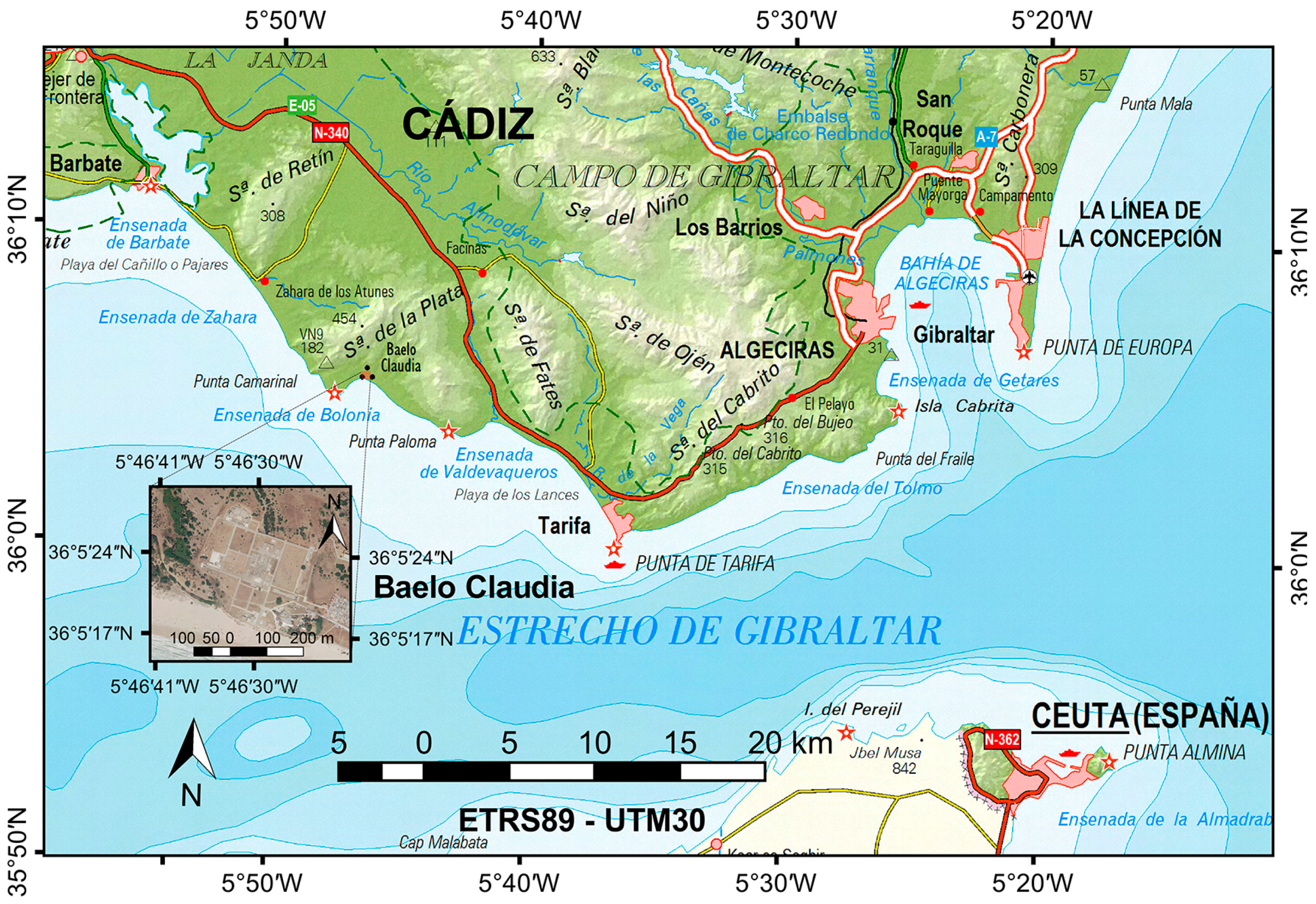
The Archaeological Ensemble of Baelo Claudia is located in the Ensenada de Bolonia (bay) in Tarifa (Cádiz, Spain), near the Strait of Gibraltar. Figure 1 shows the site location within the geographic context of the region.

The oldest archaeological evidence of the pre-Roman settlement in Baelo date from the mid-2nd century BC, prior to its consideration as a Roman municipality [31], when it was named ‘Claudia’ after the Emperor Claudio [24]. The industrial activity in this Hispanic-Roman city was the production of salt-fish, mainly tuna, garum and mixed sauces that have been found in amphorae of the Roman republican period [32,33,34]. This economic development decreased during the second half of the 2nd century AD, but the commercial activities restored the significance of the city from the 3rd to the 4th century. Afterwards, Baelo Claudia began to decline until it was completely neglected in the 7th century [35].

According to Bernal et al. [36], Baelo Claudia is a great example of the implementation of the Roman urban models in the south of Hispania, the Iberian Peninsula. The archaeological and architectural diversity in Baelo Claudia is evidenced by the existence of multiple buildings and infrastructure such as a theatre, a basilica, temples, thermal baths, macellum, factory, roads, etc.

Baelo Claudia is located in an area with a low-moderate seismic hazard, but which was affected by energetic earthquakes such as the earthquakes in Lisbon (1755) and in Cape St. Vincent (1969) [37,38].

The Archaeological Zone of Baelo Claudia and its environment were listed as a National Historic Monument in 1925 and delimited in 1991 [39]. It was constituted as the institution ‘Archaeological Ensemble of Baelo Claudia’ in 1989 by the regional government [40].

The judicial basilica of Baelo Claudia is the case study of this research. This courthouse is located in the central area of the Archaeological Ensemble, beside the decumanus maximus—the main road crossing the city southeast to southwest [41]—and between cardo 3 and cardo 4, which are the roads facing northeast, and perpendicular to the aforementioned road. There are 18 columns in the basilica—out of 20 that constituted the building in the past—standing aligned, forming a rectangle of approximately 23.3 m × 10 m, with a maximum column height of 5.5 m from ground level.

4. Methodology

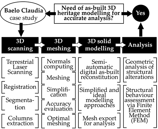
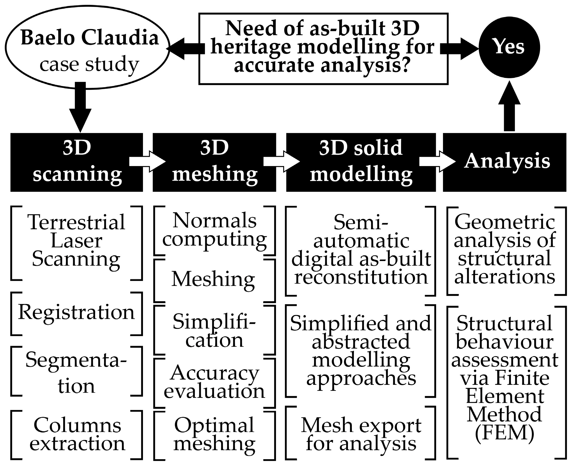
As previously stated, the methodology of this paper firstly addresses the as-built digital reconstitution of the columns of the basilica in the Baelo Claudia archaeological ensemble. The modelling methods here presented allow to obtain accurate measurements to be used in the geometric analysis (displacement, distortion and deformations of the columns and their parts), as well as for assessing the structural behaviour. Figure 2 summarises the research methodology.

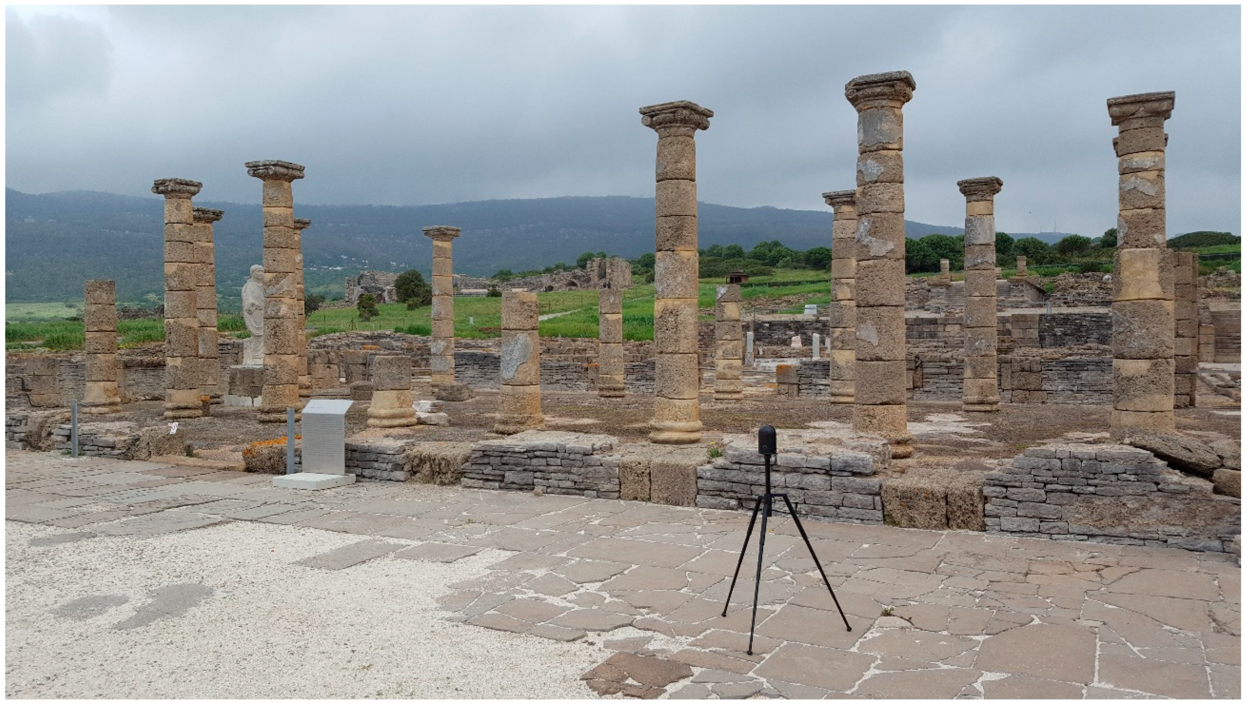
4.1. 3D Scanning

Given the dimensions and the characteristics of the basilica, the terrestrial laser scanning (TLS) technique was used to capture the geometry of the columns (Figure 3).

The device used was the BLK360 3D scanner by Leica Geosystems [42], which has a maximum range of 120 m (60 m radius), a point measurement rate of 360,000 points per second, and the accuracy of 4 mm at 10 m when the highest resolution configuration profile is selected. High dynamic range (HDR) images were also taken in the scanning to map the point cloud and the subsequent 3D meshes of the columns, although further combination of TLS with photogrammetry would enhance the digitisation of the site when high-quality texture mapping is necessary [15].

No targets were used in the survey for the 19 positions of the scanner, which were strategically defined to ease the alignment, given the sufficient overlap between those positions; i.e., the same columns were captured from different angles. An itinerary as regular as possible was established to minimise errors and point cloud quality decrease [43], in order to ensure the complete geometry capture of the columns, thus avoiding shadows in the lateral column surface due to the occlusion of the laser beam [44]. In the 3D survey, due to technical issues, both the inertial measurement unit (IMU) as tilt sensor integrated into the BLK360 laser scanner and the automatic cloud-to-cloud matching were chosen against GNSS ground control points (GCP) to create the levelled coordinate system. The different scans were imported into Leica Cyclone REGISTER 360 software [45] on a laptop computer through the Wi-Fi network of the scanner so that the alignment of those scans into the same coordinate system could be automatically performed [18]. 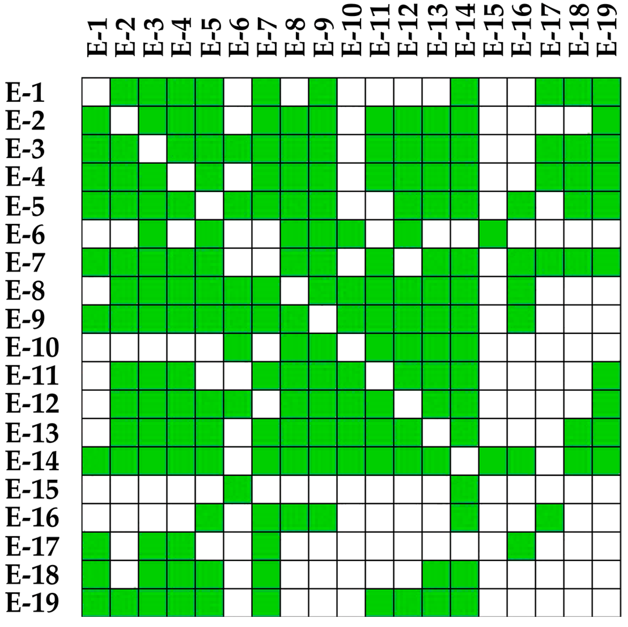This registration process [46], carried out using the auto-alignment feature in the software, automatically produced 101 scan links or connections between the different clouds (data from the different scan positions or stations). Certain registration errors were solved by performing automatic cloud-to-cloud matching. The average values in the final scan report of the survey were 81% strength, 54% overlap and 0.006 m bundle or scan group error in the global registration. Figure 4 shows the scan links automatically produced by Leica Cyclone REGISTER 360 to connect the 19 stations (scans) or scanner positions (E-× labels) appearing in the subsequent Figure 5.

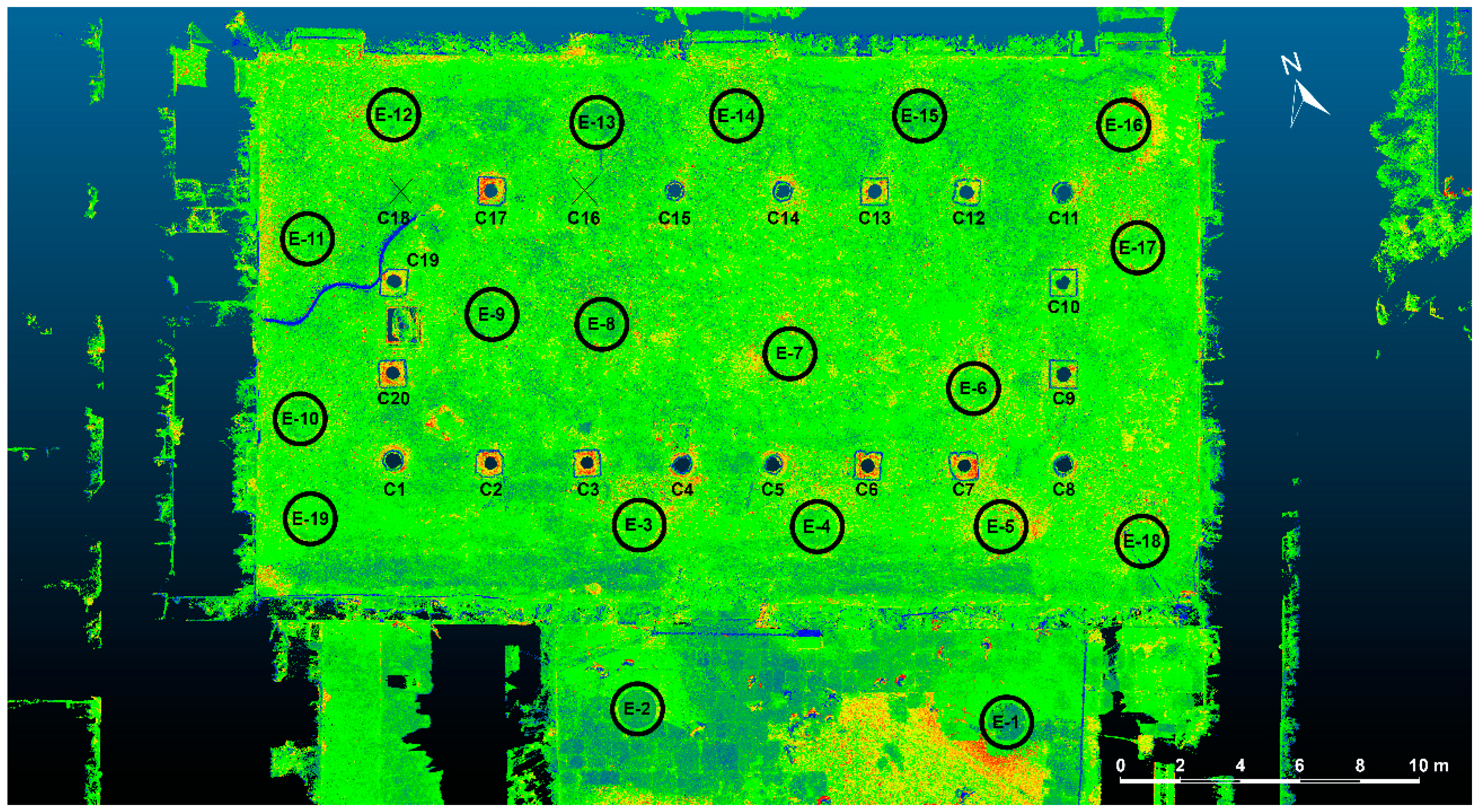
The result of this process was a massive point cloud containing approximately 426 million points for a total file size of 18.27 GB in PTS format. Figure 5 shows the numbered columns (Cx labels) and scan positions (E-x labels) within a top view of the point cloud of the basilica of Baelo Claudia and its surroundings enhanced with intensities. Naming the columns is essential for the subsequent 3D modelling and analyses addressed in this paper. It is worth saying that columns C16 and C18 are missing, as described above, but their number will be taken into account to maintain a rigorous order in this research. In Figure 5, the distances between the scan positions and the columns can be measured using the graphical scale.

Given the amount of information produced, it was necessary to perform the segmentation [47] of the global point cloud in order to reduce the number of points according to the needs of this research and then select the desired area to study, which was the group of columns in the basilica. For this task, a polygon fence was manually created on the top view to remove the surroundings of the basilica. CloudCompare [48] v2.91 for 64-bit Microsoft Windows was used to perform this manual segmentation. The resulting point cloud contained nearly 160 million points for 12.85 GB, including the ground around the columns. The cloth simulation filter (CSF) [49], integrated into CloudCompare as a plug-in, is a filtering method to detach the ground from LiDAR (light detection and ranging) data. Nevertheless, the lower parts of the column bases in the basilica were also removed with the ground data when using this algorithm. For this reason, further manual segmentation was required to remove the ground, given the fact that both its irregularity and the different levels of the columns’ bottom also made it difficult to set elevation thresholds for removal. New fences enclosing the columns allowed their extraction from the global point cloud of the basilica, thus conserving their current coordinates with a view to model and analyse them within their original context.

4.2. 3D Meshing Process and Validation Test

Once the point clouds of the columns have been segmented separately, they must be converted into triangle meshes so as to produce the 3D models for subsequent analyses. It is necessary to distinguish between these meshes—this article refers to them as 3D meshes—and FEM meshes that will be built for the structural analysis. To achieve the 3D meshing, CloudCompare software requires computing the normal vectors [50] of the point clouds. While most of the point clouds provided suitable results in normal orientation, the complexity and noise of some of them may have caused incoherent orientation in this process. In order to produce correct meshes fitting the point clouds, the normals should point outwards from the object’s volume [51], thus avoiding inverted normals (inwards). This required modifying the parameters of the computation. The optimal settings were selected by experimentally checking the suitable results of the point cloud orientation. The Plane mode was selected, with the ‘Orientation’ checkbox activated and six neighbours for each point determined.

At this point, the 3D meshing process takes place. The screened Poisson surface reconstruction by Kazhdan and Hoppe [52], which is included in CloudCompare as a plug-in, generates watertight meshes from oriented point sets (point clouds with computed normal vectors). This Poisson algorithm is chosen in this paper against other meshing algorithms, such as Marching Cubes [53], included in MeshLab software [54] as a plug-in, since the latter produced an open mesh from a sample point cloud of a column base and excessive noise to build the surface. Moreover, Marching Cubes needed significant time to conduct the meshing in comparison with Poisson (229 s against 29 s for the mesh quality considered in this research), which has greater impact on the entire digital reconstitution of the basilica of Baelo Claudia. The watertight meshing is suitable for the purpose of this research, since the absence of holes in the meshes allows the subsequent creation of closed polysurfaces (3D solids) for the as-built modelling of the columns of the basilica, described in Section 4.3. In the Poisson plug-in, different values of the Octree Depth parameter can be selected; these values entail diverse mesh quality results and number of triangles. Therefore, these aspects are qualitatively and quantitatively assessed in this research to validate the optimal 3D meshing process. High values of Octree Depth produce meshes accurately fitting the point clouds, but this may cause an excessive relief when there is noise in the point sets, which does not represent the actual geometry of the columns. The reason for this can be errors in the registration, where two or more scans overlap with insufficient fit, or caused by the laser beam error, thus producing inaccurate surfaces. In contrast, meshes configured at lower values of this parameter fit the point clouds to a lesser extent, which simplifies the discretisation excessively—the geometry becomes smoother. Nevertheless, although the achievement of mesh accuracy is the aim of this research, a certain degree of simplification is considered to decrease the number of faces (triangles) in order to enhance the processing time and reduce computational efforts in subsequent 3D modelling operations. The mesh simplification consists of reducing the number of triangles in them using specific software, such as Artec Studio 10 Professional [55]. The difference between the simplified 3D meshes is qualitatively shown in Figure 6.

With a view to validate the 3D meshing process and decide the extent of smoothening or simplification, a test is carried out for column C1 meshes, which were produced through the method by Kazhdan and Hoppe [52] in CloudCompare. To do this, a quantitative analysis of the meshing accuracy firstly compares the main features of the meshes: (i) number of vertexes (points of the clouds/meshes); (ii) number of faces (triangles, polygons); (iii) surface (area) of the meshes; (iv) average surface of their triangles; (v) volume of the meshes; and (vi) standard deviation. Secondly, it is studied the deviation between the meshes or clouds corresponding to the different simplification degrees. As a result, the optimal parameters of the 3D meshing process can be set. The results of this validation test are gathered and explained in Section 5. Results.

3D Mesh Treatment

Apart from reaching the simplification extent as described above, Artec Studio is used to optimise the 3D meshes by performing the following processes:

• Manual removal of polygons out of context, including sectors whose deformations will not be analysed, such as the remaining ground surrounding the column bases.
• Automatic watertight close of meshes with holes as a result of the aforementioned task.
• Checking of mesh defects due to triangulation errors (for instance, duplicate points and faces, naked edges, inverted normals, etc.).
• Manual brushing of visible imperfections such as bridges connecting opposite surfaces or sharp shapes. This may be caused by heterogeneous density of points in the cloud prior to meshing.

Finally, although the remeshing produces an isotropic mesh, i.e., the size and distribution of the triangles become more homogeneous, it was discarded from this research in favour of the original (simplified) meshes. The reason for this are the significant processing time that is required, the increase in the number of triangles, the consequent smoothening and, therefore, the loss of geometry relief despite that increase.

4.3. Digital Reconstitution: Solid Modelling

The aforementioned geometric analysis objective implies the need of working with separate drums and joints between them. Dealing with solid models rather than 3D meshes eases the use of Boolean operations to divide the original one-piece column into different parts. To achieve this, two processes of the semi-automatic modelling procedure as described by Antón et al. [3] within the environment of Rhinoceros V5 software [56] are firstly conducted: (1) check the integrity of the meshes, although there should not be any inconsistency, since this was already tested in Artec Studio when producing the optimal meshes; and (2) convert the watertight meshes into closed polysurfaces (solid objects).

Secondly, this paper includes manual and automatic processes to divide the complete solid column for the subsequent detailed analyses. The division of these polysurfaces is carried out by creating cutting surfaces from points inserted by the upper and lower bases of each drum near the joints. 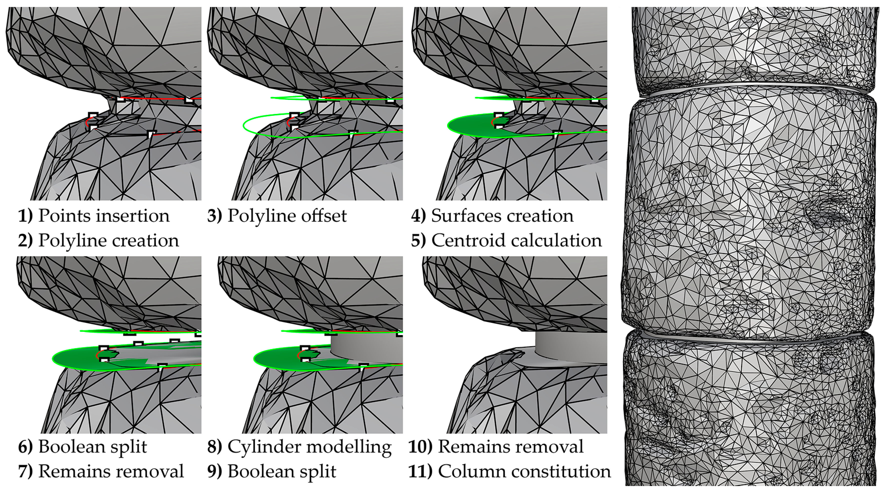Concerning the joints between drums, the capture of their geometry was not possible in the 3D survey, since the level of the scanner was lower than that of the joints hidden between higher drums, causing shadows in the point cloud [44]. Hence, it is decided to define the volume of the joints considering the cutting surfaces previously modelled and a cylinder between them. The centre of this cylinder is the centroid calculated from the surfaces. Then, it is necessary to subtract from the cylinder the volume intersecting the drums, which is performed through the Boolean split operation. Figure 7 shows the process to obtain separate drums and model joints as explained above —the six detailed figures focus the same area by the northern side of the third mortar joint of column C1 (lower joint of the right image in Figure 7).

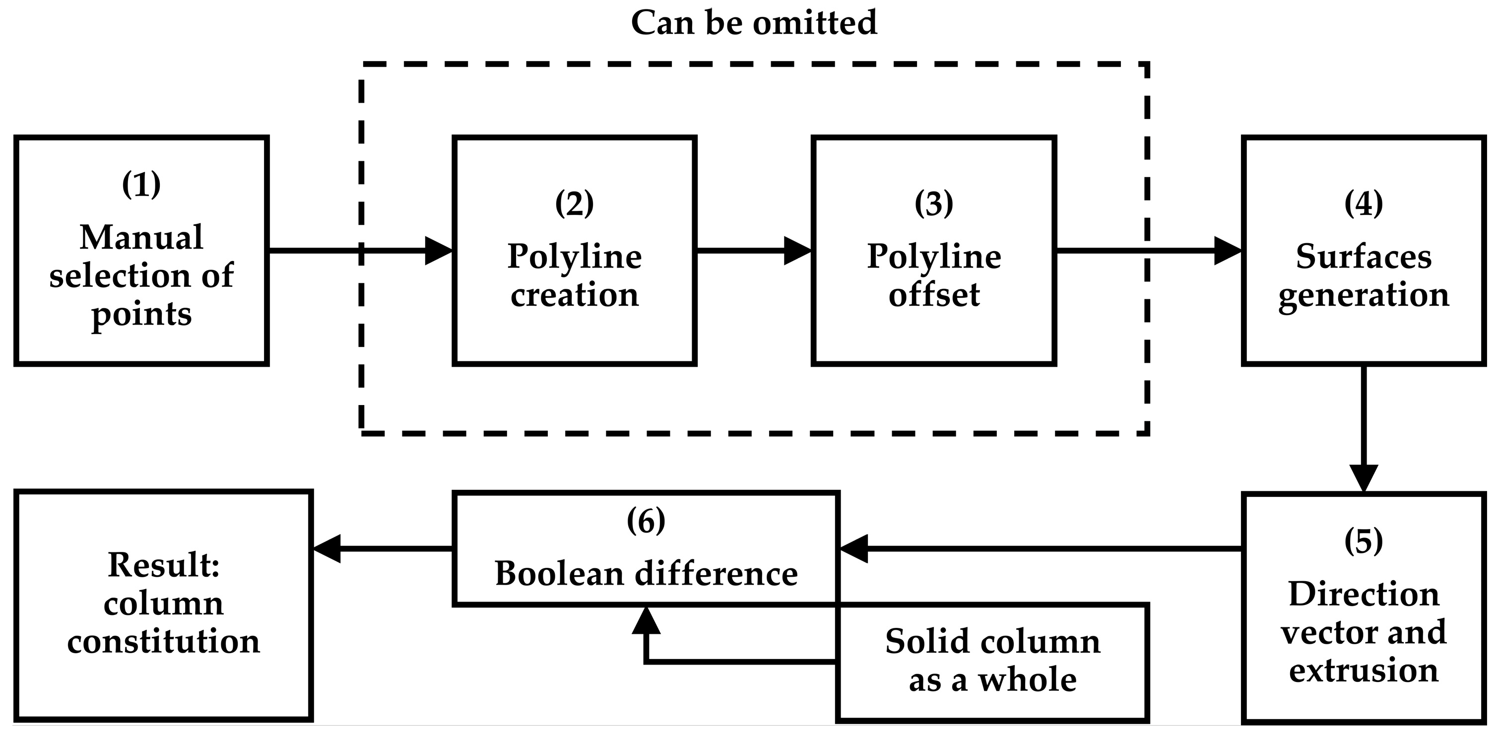
This drum splitting process can be semi-automated using a simple script within Grasshopper [57] (build 0.9.0076) environment. Grasshopper, a visual programming language for Rhinoceros 5, is a plug-in that allows intuitively creating algorithms, based on the workspace of Rhinoceros to operate the 3D model in real-time. The following script (shown as a diagram in Figure 8) was created ad hoc in this research to reproduce the processes explained above, conducted to divide the columns into parts (drums).

The script performs the following semi-automatic algorithm: (1) selection of points manually inserted on the drum edges near the joints; (2) polyline creation from those points; (3) polyline offset; (4) drum base surfaces generation; (5) surface extrusion along a given direction; and (6) Boolean difference (subtraction) operations from the entire solid column with the extrusion as an operator. Steps 2 and 3 can be omitted, since the points in step 1 can be ‘patched’ as well to produce surfaces. In order to complete the splitting process for the rest of drums, it is necessary to select the rest of the points on the drum bases and repeat the steps. The application of this script to all the columns of the basilica should save significant time in their digital reconstitution.

In this paper, it is assumed that modelling minor elements such as the joints between drums as simplified entities should not have great impact on the structural simulation, when compared to the actual geometry of the joints on site. It is also worth noting that the use of Boolean operations produces uniform and accurate contact surfaces connecting the parts, which is essential for the structural behaviour assessment [58].

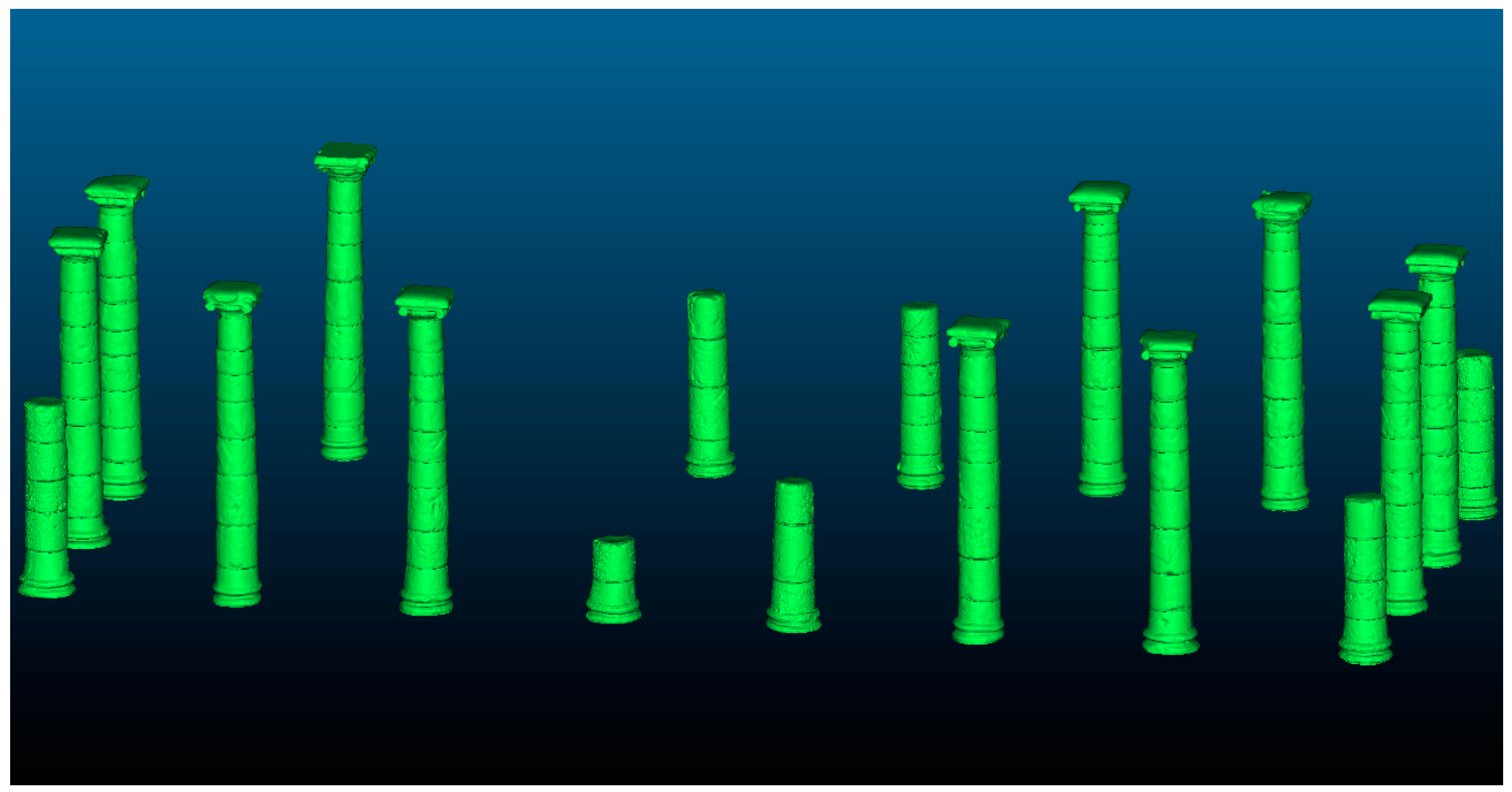
Once all the processes for the 3D meshing and solid modelling of the columns and their deformations are completed, the digital reconstitution of the basilica through as-built models can be displayed (Figure 9).

Additionally, additional modelling methods in Rhinoceros are presented to achieve the third specific objective of this research, which is to evaluate the suitability of different modelling approaches by assessing their structural behaviour. These approaches are implemented for the most unfavourable column (C19) (see Figure 5 to locate the column). The enquiry into which column is the one with greater displacements and distortions is based on the methods described in Section 4.4. Geometric Analysis. The complete results are gathered in Table S1: Displacements and distortions in columns in Supplementary Materials.

Prior to undertaking the modelling processes, it is necessary to calculate the centroids of the drum bases in the as-built model in order to maintain the exact position of the drums and the joints in both simplified and ideal models. To do this, these bases (surfaces) must be extracted from the drums. Subsequently, the base centroids needed are calculated form those surfaces.

On the one hand, the simplified approach is described. This method considers horizontal joints and drum displacements with respect to the vertical axis of the column, following traditional measurements:

• To generate three horizontal sections of the drum: one in the middle of its height to extract its general diameter; two for its lower and upper bases, respectively, to represent the diameter reduction and produce horizontal joints.
• To insert multiple points in the curves (divide the curves).
• To automatically draw a circumference fitting those points.
• To clone the middle section (circumference) to where the diameter changes with respect to the general diameter of the drum, so that the drum can be modelled as following traditional measurements.
• To match the direction of all circumferences to establish a coherent set of curves.
• To create an open fitting transition with automatic seam point orientation, straight sections, and 10 control points, selecting the circumferences at the top, bottom and the two curves where the diameter varies (four circumferences in total).
• To close the transition by covering the holes at the bottom and the top of the drums with planar surfaces to obtain closed polysurfaces (solid objects).
• To create cylinders in the joints as for the standard joint modelling method presented above, taking the base centroids as the cylinders’ centres, and their height larger than the space in the joint. To perform Boolean subtractions to remove the volume that exceeds the bases and intersects the drums.
• To section the original column capital to extract the average dimensions of the top (rectangle), middle part and bottom (circumferences), and model using primitive geometries accordingly. To perform Boolean subtraction to remove part of the volume that is missing in the capital.

On the other hand, the ideal approach without displacements is explained:

• To create three equidistant horizontal sections dividing the height of the drum into four parts.
• To generate the average/characteristic section (curve) from the three curves above two by two, matching the original ones.
• To insert multiple points in the curve (divide the curve).
• To automatically draw a circumference fitting those points.
• To create a planar surface from that circumference.
• To extrude the surface towards the base centroids to obtain the height of each drum, thus producing horizontal joints between them.
• To create cylinders in the joints, taking the base centroids as the cylinder’s centres, and their height larger than the space in the joint. Perform Boolean subtractions to remove the volume exceeding the bases.
• To section the original column capital to extract the average dimensions of the top (rectangle), middle part and bottom (circumferences) and model using primitive geometries accordingly.

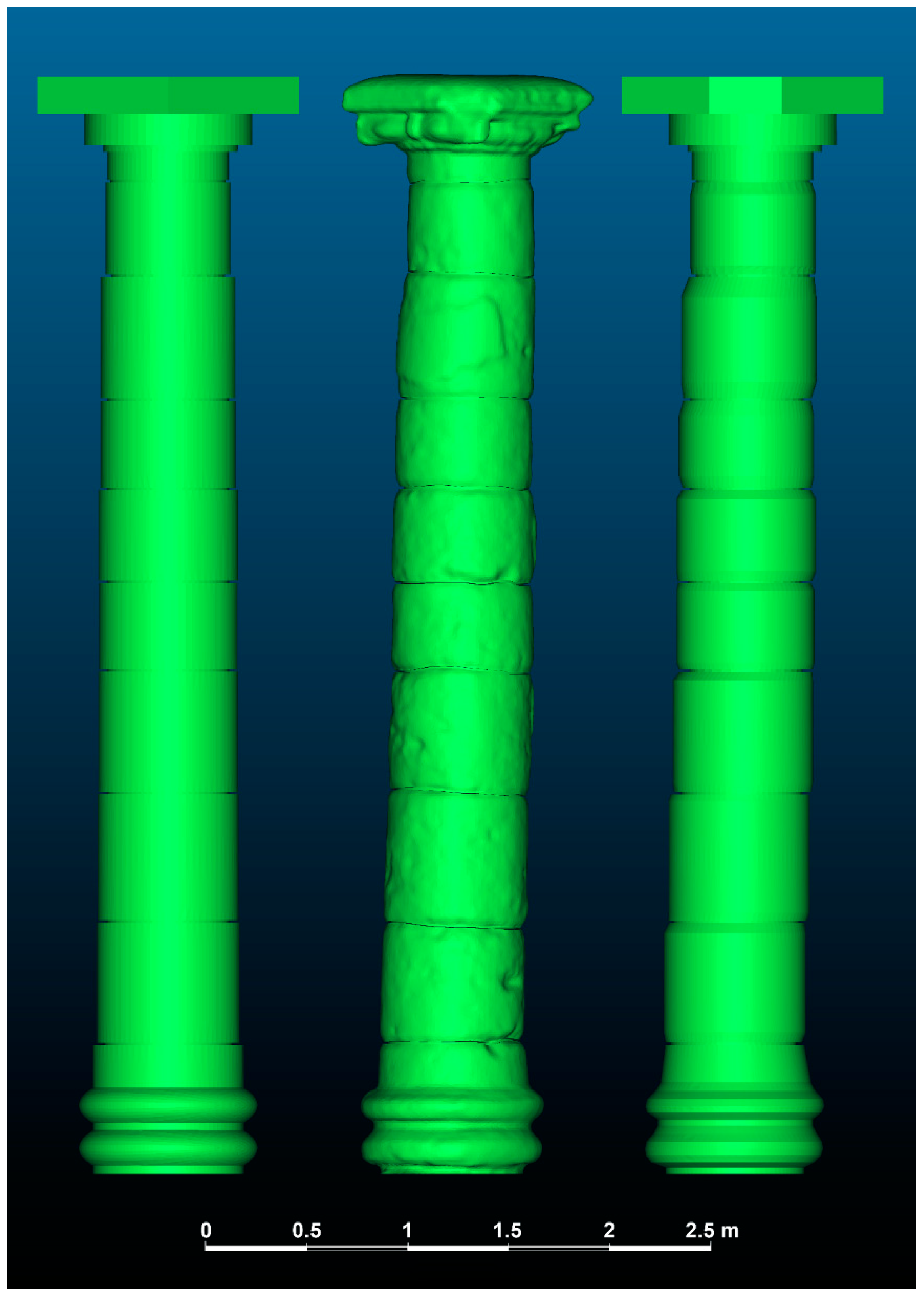
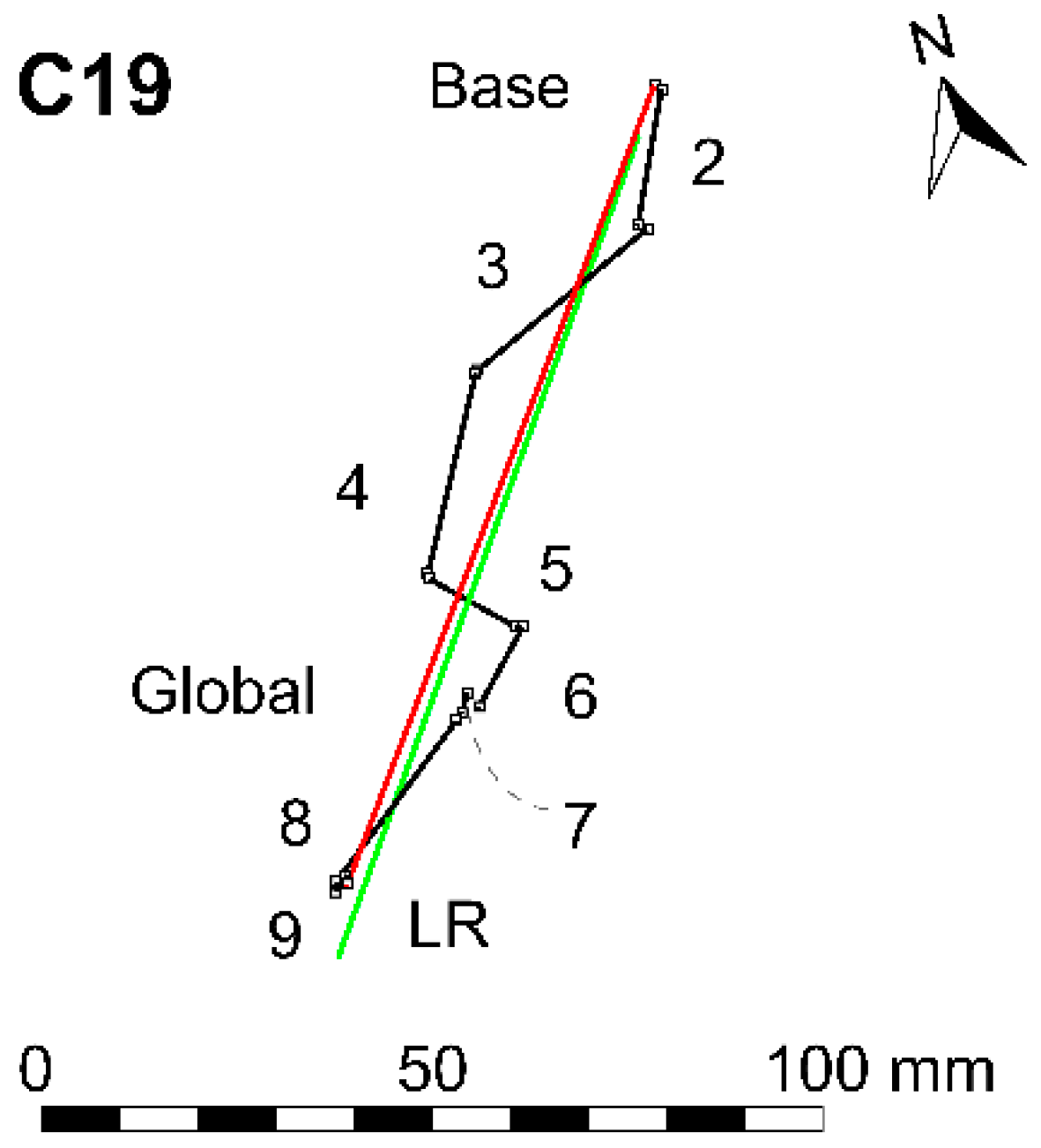
Figure 10 shows the unfavourable column (C19) modelled following different approaches: (i) the as-built column through the semi-automatic procedure proposed; (ii) the simplified model using sections by the base centroids to create transitions; and (iii) the ideal column built with transitions along the vertical axis.

Finally, the drums and joints are separately exported as STL 3D mesh format for subsequent import into ANSYS ICEM CFD 18.0 [59] to produce the FEM mesh in order to perform the structural analysis on the columns. As abovementioned—in Section 4.1. 3D Scanning—by following the proposed modelling procedure, each individual object maintains its coordinates within the same system. That eases the import procedure, since the location of the elements is automatically defined.

4.4. Geometric Analysis

This section is intended to achieve the second objective of this paper about analysing the displacement, distortion and deformations of the columns. Although the methods to extract these geometric data from the as-built models are described throughout this section, Grasshopper was also used for the calculation of the distance between the points (centroids) analysed in the drums. The Euclidean distances [60] between these points are calculated in vector space R² and gathered in Table S1 (Supplementary Materials). 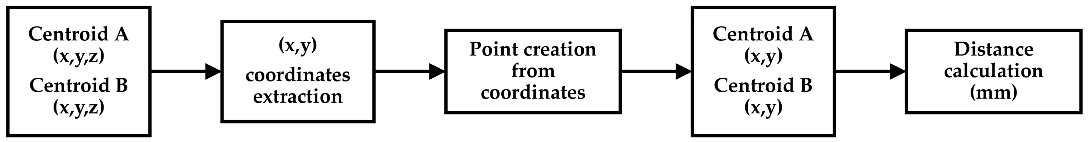The ensuing Grasshopper script (shown as a diagram in Figure 11) automates the calculation of the Euclidean distance:

This simple script was also created ad hoc in this research to measure the displacement and distortions in the drum bases and their volume centroids, respectively, in order to geometrically analyse the columns. Being intended to avoid the time-consuming manual task of measuring the distances one by one, the script performs the following semi-automatic algorithm: (1) point selection (manual); (2) extraction of X and Y coordinates; (3) creation of subsequent points on the XY plane; (4) Euclidean distance calculation; and (5) result. Basically, this procedure avoids the Z coordinate to compute the distance between those two points translated to the XY plane, given the fact that the displacements and distortions are measured in the top view.

Finally, it is also worth mentioning that the accurate modelling of the columns in the basilica allows the calculation of the surface of the 3D meshes and their average triangle area, as well as the volume of all the drums. Considering the density of the materials, the volume is essential to calculate the mass of the different drums by following Equation (1):

m = dV,

(1)

where m is the mass of the element in kg, d accounts for the density in kg/m³, and V is the volume in m³.

The surface and volume of all the drums are gathered in Table S2 (Supplementary Materials).

The specific approaches to perform the geometric analysis are described in the following Sections.

4.4.1. Displacements of Columns and Drums

The global displacement of the columns is calculated considering the centroids of the upper side of the column base and the lower base of the column capital. This procedure provides the displacement of the column axis at the top—the extent the column capital shifts from the base. Therefore, given the fact that the columns without capitals (C1, C4, C5, etc.) are not complete since they lack several drums, the general displacement calculation is not addressed in these cases. In addition, the particular displacement between the upper and lower bases of each drum is determined considering their respective base centroids.

Following a non-algorithmic measurement method as in the script (Section 4.4), the displacement could be calculated either mathematically using the coordinates of the centroids—this is essentially the aim of the script, measuring the distance between them on the horizontal plane—or geometrically by creating a vertical axis from the first centroid and measuring the distance perpendicular to it from the second point.

4.4.2. Distortions of Drums

The geometric analysis also comprises the distortion calculation of drums with respect to the vertical axis of the ideal column without deformations. To do this, both as-built and ideal columns are aligned by taking the column bases’ upper base centroids as a reference. In this way, the two column versions are placed in the same coordinate system. The developed Grasshopper script can also be applied to calculate the distance (distortion) by selecting the specific centroid and any point in that axis as a reference. Similarly, the mathematical and geometric approaches are able to measure the distance perpendicular to the ideal axis from each centroid, thus calculating their distortions. However, the drum distortion of the column capitals was not considered, given the impossibility of capturing their upper base with TLS and, therefore, of modelling them accurately. In this way, calculating the volume centroid of the capitals would entail significant errors. The distortion measurement of their lower bases is approximated instead.

In addition, it is worth considering the distortions of the drums in relation to the drums that are located below, which constitutes the eccentricity of these parts. The calculation using the script is simple, since it only requires selecting the volume centroid of each drum to display the distance between them on the XY plane. This provides a direct insight into which drums shift the most from each other.

4.4.3. Deformations of Drums

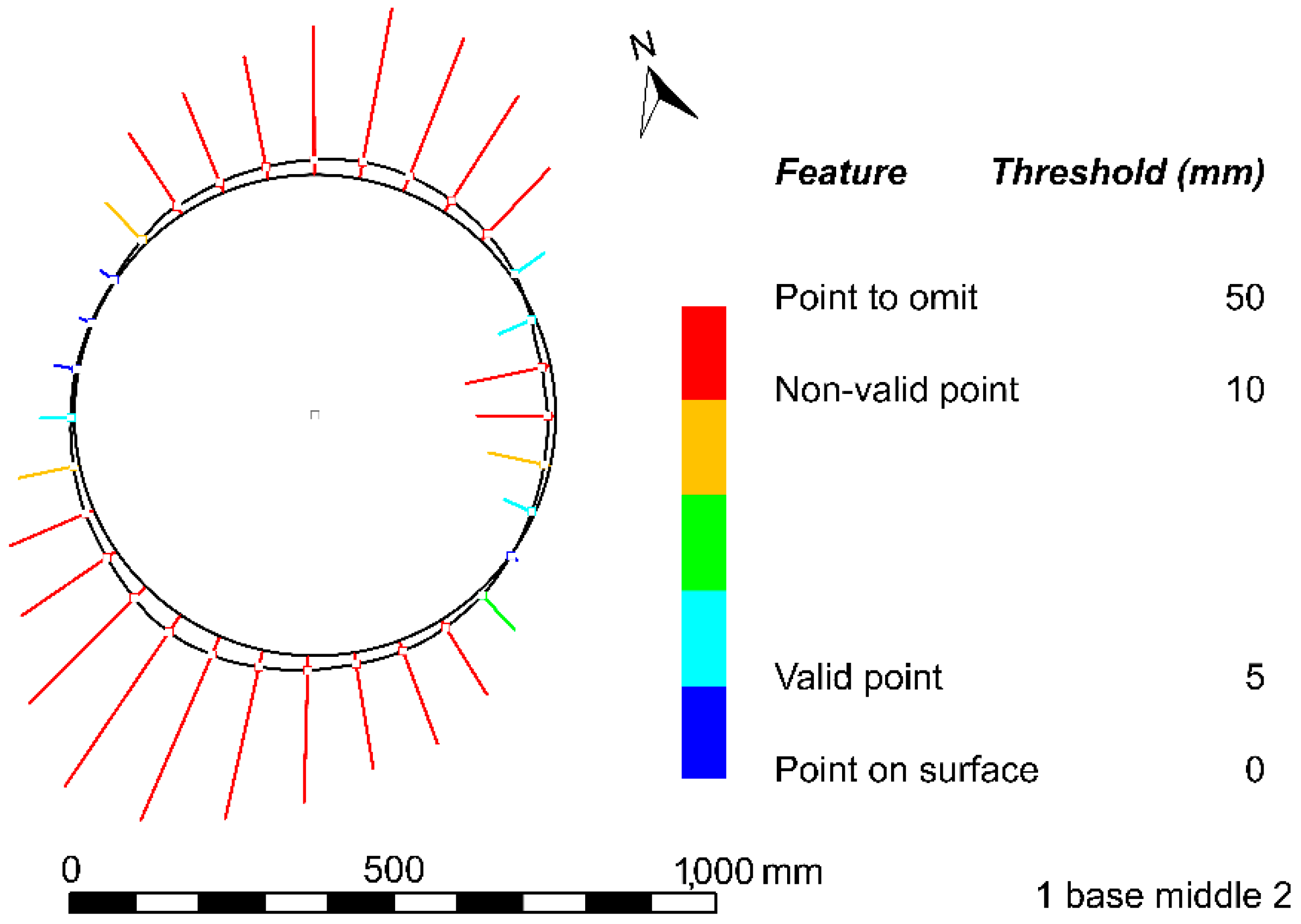
The surface deformations of the drums are also quantitatively analysed. This is carried out for the unfavourable column C19, which is studied in detail. As seen in Figure 10, the as-built models take into account the deformations of the columns, whereas the ideal modelling approach considers surfaces based on primitive geometries but containing their overall dimensions. In this way, the analysis of different sections of both models for each drum provides an insight of the irregularities of the as-built surface and, thus, allows the identification of parts to be restored. To do this, both models need to be aligned. The proposed methodology for the digital reconstitution guarantees that all the elements of the basilica maintain their original position within the same coordinate system. The alignment of the as-built drums is then automatically performed. However, the ideal modelling was conducted separately to ease the workflow. Therefore, it is necessary to align the ideal drums with the as-built components drum by drum, as if there is no distortion with respect to the vertical axis. The volume centroids of the as-built drums and the centre of the ideal sections (circumferences) are aligned. The horizontal sections of the drums are created in three levels—lower, middle, and upper—and named accordingly, but in the case of the more complex column bases, for which a second middle section is given. The deviation of points within the curves (sections) is analysed. These points can be directly extracted from the polysurfaces (solids), but it is considered that the insertion of 32 points on the as-built sections allows a clear interpretation of the deformations. These points, numbered and aligned with the quadrant of the ideal sections, ease the identification of weak parts in the drums.

Subsequently, the distance between the sections aligned is measured. These curves intersect with each other, because the as-built sections are not regular. With a view to distinguish between areas where the points in the as-built section are located either under the ideal section—negative distances (x < 0) are considered—or over it—positive distances (x > 0)—it is worth splitting the as-built curve with the ideal one. Then, the minimum and maximum distances between them, respectively, are computed.

In addition, the general deviation between both sections is calculated in Rhinoceros. The distances from the points inserted in the as-built curve to the ideal curve (circumference) are analysed in order to obtain statistical measurements on the drum deformations, such as the average, the median and the standard deviation.

The deformation analysis of all the sections in column C19 are collected in Figure S2 (Supplementary Materials).

4.5. Structural Modelling and Analysis

In order to determine the column structural performance, focusing both on the accuracy and suitability of the geometric model, static and modal analyses are carried out on the 3D models by means of FEM. The numerical meshes are generated with the software ANSYS-ICEM v.14 [59] and the finite element software ANSYS [61] is used to build the numerical models and to analyse the structural performance.

These numerical analyses are prior and crucial steps aimed at controlling the structural response, and they allow for:

• Understanding the general structural behaviour;
• Detecting structural weaknesses;
• Obtaining the main dynamic properties;
• Determining the accuracy level of the different geometric models.

4.5.1. 3D FEM Mesh Generation

For the objective of FEM modelling, column C19 has been meshed with hexahedral elements with the software ANSYS-ICEM CFD hexa [59]. The geometry in STL format has been imported from the output of Rhino software, as described in Section 4.3.

As explained for Figure 10 in Section 4.3, three different geometries have been modelled (their names have been adapted to the common structural terminology):

• As-built model: the real geometry as obtained with the laser measuring system (Figure 10, centre).
• Simplified model: the geometry as can be measured by conventional measuring methods (Figure 10, right, where leaning is accounted for, but neither distortion nor geometry imperfections).
• Ideal model: the geometry representing an ideal column, without any damage, distortion or leaning (Figure 10, left).

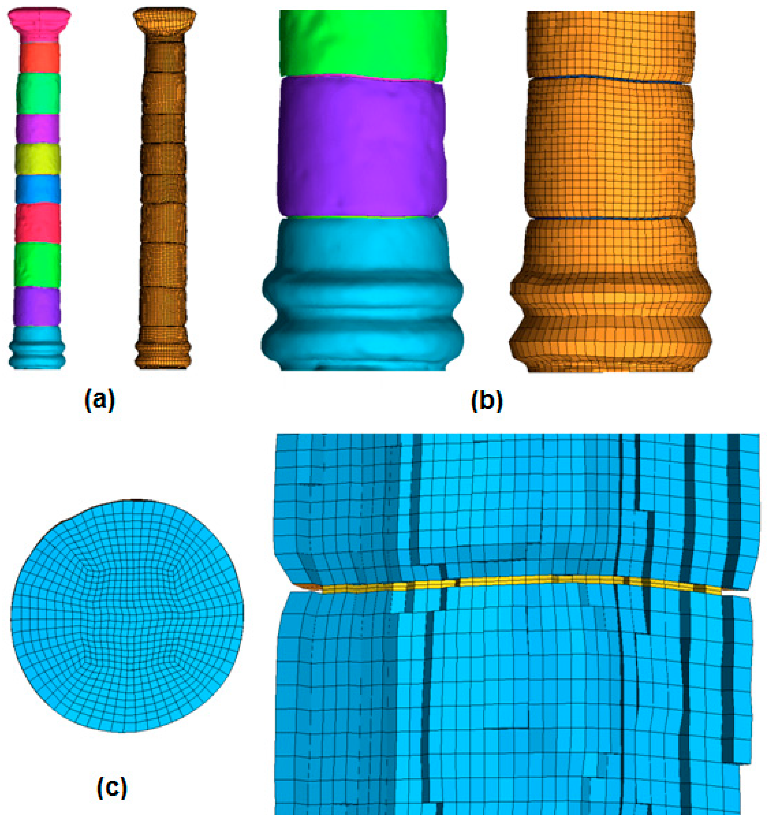
Regarding the as-built model, a general view of the imported geometry and resulting surface mesh is depicted in Figure 12a, with a detailed view in Figure 12b. Figure 12c presents the internal 3D mesh (slice plane and detail of a front view). The O-grid topology was used to correctly mesh the cylindrically-shaped geometry with an appropriate mesh quality (see Figure 12c).

Column C19 has been meshed with a total of 174,360 hexahedral elements (153,284 nodes). The number of mesh elements in the height of each drum is 20, as well as in the capital and base. Two elements were used for the height of the mortar joint thickness, where the average height of the mortar thickness is 12 mm. The average hexahedral element face angle is above 75°, but due to the complexity of the capital (in particular in the as-built geometry), a few elements with smaller angles are present, featuring a minimum value of 18º. The minimum aspect ratio of the mesh elements (size of the minimum element edge divided by the size of the maximum element edge) is 0.05, and the minimum skewness is 0.15. Highest mesh expansion factor is 45. The average mesh resolution (Δ_x) is 3 mm, which is ensuring an appropriate mesh refinement for the structure under analysis. It must be considered that the mesh resolution is having an impact on the FEM results and, thus, a mesh independence study is generally required for ensuring accurate FEM results. All three geometries were meshed with the same parameters and, therefore, the number of elements and nodes, and the overall mesh resolution are the same for all the modelled geometries.

4.5.2. 3D FEM Structural Modelling and Analysis

After modelling the three 3D FEM mesh (as-built, simplified and ideal), 3D FEM structural models are built, and the three column models are numerically tested and compared.

Three-dimensional eight-node solid elements, SOLID 65, are implemented within the mesh. The SOLID 65 element comprises eight nodes, having three degrees of freedom at each node: translations in the nodal x, y, and z directions.

The structural numerical analyses are carried out under gravity loading. The structural performance is analysed in the linear range, focusing on the ultimate limit state verification. Although, the nonlinear approach is the reference analysis for comprehensive safety assessments, the linear range makes possible to obtain significant data from both a qualitative and a general quantitative perspective [62,63]. Additionally, the linear analyses are the preliminary and necessary steps for future comprehensive assessments under dynamic loading and aging phenomena [64]. Taking into account the main scope of this work, the data provided by the linear range are of special interest.

A macro-model with homogenized properties is implemented into the mathematical formulation. A smeared model is assumed, considering that the structural materials are initially isotropic until either one of the tensile or the compressive strength are exceeded. Thus, stone units, mortar and interfaces are smeared out in the continuum, and the damage pattern is inserted in the model by adjusting the stress-strain matrix.

The material control parameters of the 3D-solid models are determined on the basis of the material properties that were obtained in previous research [24,65]. The structural materials are calcarenite stone (capital, base and drums) and lime mortar (joints). From the aforementioned, the specific weight w is equal to 21,000 N/m³, the Young modulus E is equal to 2 × 10⁹ N/m², and the Poisson ratio ν is equal to 0.2.

As far as boundary conditions are concerned, the base of the C19 column is completely constrained.

In order to verify the ultimate limit states, static analyses are performed, following the Eurocode prescriptions [66]. In addition, modal (eigenvalue) analyses are also carried out in order to obtain the dynamic properties—natural frequencies, ω_n, and modal shapes, ζ_n.

After performing the numerical analyses via FEM, the compliance factor α is obtained. With that factor, the resistance or the deformation capacity (related to the ultimate limit state, in correspondence to the compressive strength values) is proportioned to the gravity loading effects (α = R/D). If the compliance factor α reaches a value larger than or equal to one, the safety requirements are completely fulfilled.

In addition, the stress-strain gradients are compared, as well as the maximum value variations (in terms of stress-displacement fields) among the models. The α factor and the comparative analyses provide valuable data both on the accuracy and suitability of each model.

5. Results

The outcomes deriving from the different sections containing quantitative data are presented here by following the structure of the methodology: (i) 3D meshing and its evaluation; (ii) geometric analysis, comprising the calculation of displacements, distortions and deformations of columns and drums; and (iii) structural behaviour assessment of the three modelling approaches for the most unfavourable column.

5.1. 3D Meshing Process Validation Test

The validation test of the 3D meshing process explained in Section 4.2 constitute a quantitative analysis of the features of the original column meshes—those produced directly from the point cloud—the meshes simplified to diverse degrees, and the original point cloud (

Table 1. Quantitative analysis of the meshing accuracy in column C1.

Object	Octree Depth	Number of Points	Number of Faces	Mesh Surface (m2)	Average Triangle Surface (m2)	Mesh Volume (m3)	Standard Deviation (Points)
Mesh 0	8	62,520	125,040	12.163	9.727 × 10−5	1.582	136.895
Mesh 1	9	257,188	514,392	12.693	2.468 × 10−5	1.612	4432.056
Mesh 2	9 simplified	49,992	100,000	12.655	1.265 × 10−4	1.612	239.839
Mesh 3	9 simplified	24,992	50,000	12.617	2.523 × 10−4	1.611	57.926
Mesh 4	9 simplified	9992	20,000	12.535	6.268 × 10−4	1.607	10.639
PointCloud	--	2,013,465	--	--	--	--	--

).

The mesh features gathered in Table 1 are calculated using CloudCompare, except for the standard deviation, which accounts for the dispersion of points with respect to the distance intervals in the subsequent Figure 13, Figure 14 and Figure 15. From the table, given the significant geometry loss in terms of surface and volume of meshes 0 and 4, these degrees of smoothening and simplification, respectively, are dismissed. The digital reconstitution of the basilica according to those parameters would produce columns with excessive simplification. On the other hand, higher Octree Depths such as level 10 onwards produced an excessive number of triangles and vertexes—level 11 created more points than those existing in the original point cloud—as well as noise on the column surface, thus reducing the mesh quality as the same time as the computational resources demand in processing, subsequent modelling and FEM meshing, and visualisation increases. For this reason, it is worth presenting the meshing accuracy of mesh 1 approach (Octree Depth 9), which is used in this research to produce the meshes to be later slightly simplified with a view to reduce the computational effort during the digital reconstitution. This is calculated using the cloud-to-mesh feature in CloudCompare to determine the deviation between the original point cloud and mesh 1 for the sample column C1 (Figure 13).

In addition, the deviation between points of the simplified meshes 2 and 3 is respectively analysed in relation to the original mesh (1) (Figure 14 and Figure 15).

The abscissa axis in these graphs represents the point deviation between the 3D meshes (or between meshes and point clouds) divided into intervals. The ordinate axis shows the number of points or vertexes contained in those intervals. The high number of points in the central value (zero) indicates the null distance between homologous points of both meshes (or comparing a point cloud and a mesh), which means that the 3D objects compared are similar. Additionally, as explained by Antón et al. [3], lower values of the standard deviation mean less similarity between the compared and the reference meshes, whereas higher values account for greater similarity. The deviation graphs complement the standard deviation to show the location of the majority of points (zero value). The standard deviation, as a dispersion measurement statistical tool, is considered valid in this research to evaluate the similarity between the 3D objects since the compared simplified meshes derive from the reference meshes (or original point cloud as for mesh 0), given the simplification process required to produce the meshes (or smoothening through different Octree level). On the one hand, in order to analyse the meshing accuracy in this research, both the geometric features in Table 1 and the highest standard deviation of mesh 1 from the original point cloud (4432.056 points) in comparison with mesh 0 (Octree Depth 8) indicate the suitability of the former meshing approach. Moreover, the geometric features of mesh 0 are poorer than those of mesh 2 (mesh 1 simplified). On the other hand, meshes 2 and 3 are compared. The scale is constant in both graphs to ease comprehension. A higher similarity between meshes is more evident in Figure 14, since the points in Figure 15 are more dispersed; in the former (mesh 2), the standard deviation is 202.23 points when interpolating the zero value in the intervals, while in the latter (mesh 3), the standard deviation decreases to 49.23 points. In addition, considering the extreme intervals in both cases, the highest deviation of mesh 2 (maximum distance between the compare and reference meshes) is 0.89 mm, while mesh 3 reaches 1.49 mm in relation to the original mesh 1. These results show the inaccuracy of mesh 3, which is not considered for modelling in this work. It is also worth noting the difference between the point-cloud-to-mesh (Figure 13) and mesh-to-mesh (Figure 14) deviation graphs. There are more points in the intervals surrounding the zero value in the point cloud meshing (mesh 1 from point cloud, in Figure 13) than in those of the mesh simplification (mesh 2 from mesh 1, in Figure 14). Finally, taking into consideration the outcomes from this 3D meshing process validation test, it can be stated that the simplification degree for mesh 2 (from Octree Depth level 9) is optimal to model the deformations and the columns in the basilica, although the number of points should be proportionally defined according to the number of drums in the columns. In the case of C1, which has 5 drums, the total of 100,000 triangles per column leads to set a simplification threshold at 20,000 triangles per drum for accurate column modelling in the case study.

5.2. Geometric Analysis

5.2.1. Displacements and Distortions of Columns and Drums

The results of the geometric analysis regarding displacements and distortions calculation of all the columns and their drums as in Section 4.4.1. and Section 4.4.2. are gathered in Table S1 (Supplementary Materials). A colour scale is jointly applied to the displacement and distortion values of all the columns and drums, so that the greatest centroid deviations—the greatest drum alterations—can be individually, easily identified within the whole context of the basilica. The outcomes of the enquiry into the displacements and distortions of the as-built models reveal the unfavourable column (C19), to which both the deformations analysis and structural behaviour assessment are addressed. The global displacement of this column and the average distortion of its drums are calculated and given in

Table 2. Displacement analysis.

Column	Part/Drum	Displacement (mm)
C19	1 base	--
	2	17.56
	3	28.19
	4	26.41
	5	12.54
	6	11.70
	7	2.53
	8	25.73
	9	2.33
	10 capital	--
	Global	109.65

and

Table 3. Distortion analysis in column C19.

Drum	Centroid	Distortion (mm)
	Inferior	1.06
2	Volume centroid	8.53
	Superior	17.96
	Inferior	18.42
3	Volume centroid	26.54
	Superior	42.88
	Inferior	43.42
4	Volume centroid	55.48
	Superior	68.98
	Inferior	69.53
5	Volume centroid	71.69
	Superior	71.59
	Inferior	71.35
6	Volume centroid	78.35
	Superior	82.70
	Inferior	81.40
7	Volume centroid	84.08
	Superior	83.93
	Inferior	85.26
8	Volume centroid	92.65
	Superior	109.86
	Inferior	111.10
9	Volume centroid	113.37
	Superior	108.82
---	Average	66.62

.

The results of the eccentricity analysis of drums—distortion of the drums in relation to the parts below—are also given (

Table 4. Eccentricity analysis in column C19.

Drum	Element	Distortion Below (mm)
2	Volume centroid	14.28
3	Volume centroid	19.30
4	Volume centroid	29.24
5	Volume centroid	19.00
6	Volume centroid	7.81
7	Volume centroid	5.85
8	Volume centroid	10.80
9	Volume centroid	23.91
---	Average	109.65

).

On the other hand, the top-view representation of the complete as-built columns—those with capital—enables the displacement analysis. The as-built columns’ tilt is calculated against the ideal, vertical axis. The considered centroids are the same as in the calculation of the global (red line) and particular displacements (black lines): the upper side of the column base, each drum base (numbers), and the lower base of the column capital (see Figure 16).

The representation of the displacements of all the complete columns and their drums as in Figure 16 are gathered in Figure S1 (Supplementary Materials).

Selecting all these points (base centroids) in the column, it is possible to calculate the graphical linear regression (‘LR’ green segment in Figure 16) from them in Rhinoceros. This provides an approximated insight into the direction of column leaning. On this basis, according to the orientation of the archaeological site given by Fincker et al. [41], the azimuth of the global leaning of the columns with capitals can be calculated taking the south direction as a reference. This is shown in

Table 5. Leaning orientation of columns.

Column	Orientation	Azimuth (from South) (°)	Global Displacement (mm)
2	Southwest	−26.99	71.94
3	Southwest	−7.75	38.54
6	Southeast	14.99	20.11
7	Southwest	−21.24	45.22
9	Southeast	44.80	19.89
10	Southeast	62.40	25.22
12	Southwest	−43.54	17.25
13	Southeast	58.00	13.18
17	Southeast	41.49	66.64
19	Southwest	−39.64	109.65
20	Southwest	−37.14	92.18

.

It is worth noting that all the considered columns lean towards the coast, six of them especially to the southwest, whereas five lean southeast.

5.2.2. Deformations of Columns

Concerning the drum deformations, the results of the Section 4.4.3 are shown in Figure 17, focusing on a representative section in column C19. The deformation analysis of all the sections in column C19 are collected in Figure S2 (Supplementary Materials).

The extension of the colour scale depends on threshold values to be set according to the criteria of the specialists. In this research, considering the width or diameter of the columns, the mean and median distance, as well as the standard deviation obtained from the deformation analysis in Rhinoceros, the thresholds are set to 5 mm and 10 mm for the valid and non-valid points in the as-built sections, respectively. The points beyond the 50 mm limit are not considered in this analysis.

The statistics for the deviation analysis of the points in the real drum sections in relation to the ideal curves (deformation analysis) are given in

Table 6. Deviation analysis of as-built and ideal drum sections in column C19.

Drum	Section	Minimum Distance (mm)	Maximum Distance (mm)	Points over Surface (units)	Points under Surface (units)	Mean Distance (mm)	Median Distance (mm)	Standard Deviation (mm)
	Lower	−15.57	13.42	18	14	7.03	6.46	4.06
1.Base	Middle1	−14.68	33.20	27	5	14.85	14.60	8.77
	Middle2	−36.19	29.21	17	15	12.69	12.23	7.77
	Upper	−23.75	10.96	8	24	11.38	12.42	7.22
	Lower	−2.60	10.18	24	8	4.68	4.77	2.95
2	Middle	−28.07	7.40	17	15	4.35	3.46	4.98
	Upper	−13.47	7.98	12	20	4.78	4.12	2.83
	Lower	−7.54	9.36	19	13	3.64	3.01	2.54
3	Middle	−7.70	10.30	15	17	3.10	2.41	2.50
	Upper	−11.56	16.22	14	18	4.55	3.08	4.00
	Lower	−11.59	16.42	21	11	6.73	5.94	4.77
4	Middle	−8.93	14.74	18	14	4.95	4.16	3.26
	Upper	−10.70	20.01	20	12	5.95	5.28	5.00
	Lower	−7.45	10.38	23	9	4.33	4.11	3.28
5	Middle	−12.13	8.48	14	18	3.83	3.16	2.42
	Upper	−10.36	6.48	11	21	3.89	3.67	2.91
	Lower	−6.15	16.75	21	11	4.30	2.92	3.64
6	Middle	−4.64	16.90	18	14	2.94	1.38	4.06
	Upper	−6.33	16.40	9	23	3.19	2.36	3.37
	Lower	−10.84	11.46	18	14	4.32	4.10	3.00
7	Middle	−9.41	9.09	20	12	4.66	4.92	2.42
	Upper	−11.56	7.28	14	18	4.59	4.21	3.12
	Lower	−15.72	20.83	13	19	8.26	5.52	6.28
8	Middle	−13.97	14.15	19	13	6.56	6.57	3.75
	Upper	−15.87	18.84	7	25	7.73	6.71	4.78
	Lower	−6.51	8.77	14	18	2.68	1.64	2.49
9	Middle	−5.59	10.53	14	18	4.08	3.05	2.94
	Upper	−9.70	10.31	10	22	5.15	5.14	2.75

. This analysis is carried out in the drums of column C19, including the base and excluding the capital.

The performed analysis to obtain Figure 17 and Table 6, together with the colour scales depending on the values, indicate the specific deformations of the drums in an intuitive way. Here, the standard deviation in mm accounts for the traditional dispersion measurement of the points in relation to the ideal or ideal drum sections (Figure 17). According to the results from Table 6, considering the median distance, and the standard deviation, as well as the minimum and maximum distance from the ideal sections, both the middle and upper sections of the base of column C19 are the areas with greatest alterations in their surface/shape, especially in their north and south faces.

Finally, as stated in Section 4.4, the area of the 3D meshes and their average triangles, as well as the volume of the drums are calculated and gathered in Table S2 (Supplementary Materials).

5.3. Structural Performance

Figure 18 summarises the main results from the static analyses, providing the maximum values of the stress and displacement fields. Those results are essential in order to:

• Assess the structural response, determining areas that are prone to undergo local or global collapse;
• Identify the strongest and weakest structural directions.
• Determine the confidence threshold of each numerical model in terms of compliance factor.

In the displacement field (Figure 19), the column tilt, which is taken into account in the as-built and simplified models, causes the main differences. In the ideal model, the maximum displacement is in the vertical axis (0.0017 m u_z), but in the simplified and as-built models the highest values are located in the horizontal axis y (0.0092 m and 0.0082 m, respectively). It is worth noting that the differences between the simplified and as-built models are more relevant in the stress field than in the displacement field (8% u_x decrease, 6% u_y decrease and 6% u_z decrease, considering the simplified model as the reference).

From the static numerical results, it may be observed that although the maximum compressive levels are reached in the base area, as expected, the stress distribution and values are different (Figure 20). Obviously, the column tilt yields significant variations between the ideal model (maximum compressive level, 0.535 × 10⁷ N/m², is reached in the base), and the as-built and simplified ones (maximum levels, 0.101 × 10⁸ N/m² and 0.896 × 10⁷ N/m² are located in the joints). The lean also has a strong effect on the stress distributions, being more unfavourable those of the as-built and simplified models. Focusing on the aforementioned FEM models, although the principal stress S3 distributions are almost equal, the as-built based model exhibits higher values than the simplified one (13% increase in the maximum S3 with respect to the simplified one).

Regarding shear stresses, significant differences are obtained. The maximum values, which are quite similar for the most realistic models (1.6 × 10⁶ N/m² for the simplified one and 1.4 × 10⁶ N/m² in the as-built model), are provided by the Syz. However, the most remarkable result is the Sxz variation between the simplified and the as-built model (50% increase in the as-built model, as shown in Figure 21). That variation could be highly significant, in terms of safety compliance, under dynamic loading.

Focusing on the modal analysis results, the values of the main periods are quite similar, as shown in

Table 7. Modal results: Main periods.

	Period T (s)
Mode No	Ideal	Simplified	As-built
1	1.01390	1.02190	1.02350
2	1.01290	1.02060	1.01420
3	0.18056	0.18888	0.18261
4	0.18033	0.18846	0.18020
5	0.11966	0.11905	0.11822
6	0.07204	0.07268	0.07230
7	0.07063	0.07207	0.07054
8	0.07051	0.07161	0.06967
9	0.04297	0.04302	0.04269
10	0.03989	0.04060	0.03962
11	0.03973	0.04023	0.03928
12	0.02649	0.02697	0.02625
13	0.02635	0.02666	0.02608
14	0.02516	0.02546	0.02523
15	0.02500	0.02532	0.02469
16	0.01943	0.01978	0.01919
17	0.01931	0.01947	0.01907
18	0.01728	0.01747	0.01706
19	0.01544	0.01558	0.01529
20	0.01520	0.01541	0.01491

. Neither the stiffness degradation—due to the lack of material—nor the geometric imperfections—leaning and distortions—have provoked a significant period increase. Indeed, in the 1st mode, the period of the as-built model is almost equal to that of the ideal one (only 0.79% increase).

In

Table 8. Modal results: Effective masses (the highest values are highlighted).

Effective Masses, Meff (%)
	Ideal			Simplified			As-built
Mode No	x-Direction	y-Direction	z-Direction	x-Direction	y-Direction	z-Direction	x-Direction	y-Direction	z-Direction
1	13.26	42.31	0.00	52.75	2.73	0.01	47.14	9.13	0.00
2	42.32	13.25	0.00	2.74	52.72	0.03	9.12	47.04	0.03
3	0.03	19.21	0.00	15.76	3.77	0.02	16.26	2.98	0.00
4	19.21	0.03	0.00	3.79	15.74	0.02	2.96	16.36	0.04
5	0.00	0.00	0.00	0.00	0.00	0.00	0.01	0.00	0.00
6	0.01	0.03	75.47	0.04	1.12	68.54	0.08	0.85	70.57
7	0.30	7.30	0.23	4.87	2.61	0.52	6.85	0.47	3.02
8	7.32	0.29	0.13	2.77	4.01	6.45	0.67	6.41	2.59
9	0.00	0.00	0.00	0.03	0.04	0.00	0.06	0.01	0.00
10	0.03	4.38	0.00	2.54	1.98	0.02	3.16	1.24	0.01
11	4.41	0.03	0.00	1.97	2.51	0.04	1.27	3.19	0.02
12	0.01	2.94	0.02	1.42	1.47	0.06	2.57	0.30	0.13
13	2.95	0.01	0.02	1.42	1.44	0.36	0.30	2.59	0.10
14	0.00	0.01	9.72	0.07	0.01	9.98	0.03	0.02	9.70
15	0.00	0.00	0.00	0.00	0.00	0.01	0.00	0.00	0.00
16	0.01	2.12	0.00	1.04	1.12	0.02	1.82	0.28	0.01
17	2.12	0.01	0.00	1.13	1.05	0.02	0.27	1.79	0.01
18	0.00	0.00	0.00	0.00	0.00	0.00	0.00	0.00	0.00
19	0.02	0.08	3.85	0.31	0.04	2.98	0.04	0.02	3.92
20	0.04	1.40	0.17	0.38	0.76	0.65	1.33	0.09	0.06

, the effective masses are provided. Those mass values allow for distinguishing among the most significant modal shapes, which are those with the highest mass contribution. The most remarkable difference among values, is that, as expected, the leaning leads to a minimum effective mass redistribution among the horizontal axis x and y, being modes nos. 1 and 2 the most relevant. It is worth noting that in spite of the differences in the axis distribution, the structural response that can be assumed from those results is almost equivalent. Additionally, those results perfectly match the expected behaviour from the geometric features of the models, as the modal shape describes the configuration into which the column will naturally displace. In the three models, the first four modal shapes provide the highest mass contribution in the x and y directions. In the vertical direction, the highest value is obtained in the 14th mode.

The modal shapes are provided in Figure 22. In those shapes, the sum of the effective modal masses is more than the 90% of the total column mass. The 1st, 2nd and 4th modes involve global bending, and the modes that display torsional response are not representative (e.g., around 0.01% effective mass contribution in mode no. 15). The 3rd modal shapes provide significant out-of-plane deformations. The 6th and 14th modal shapes provide bending and translation in the vertical direction. The most representative shapes are characterized by a high global monolithic behaviour among drums and capital, and the highest stiffness is in the base area. It is worth noting that at higher frequencies (e.g., mode no. 16) the capital seems to be vulnerable, but in those cases the mass contribution is quite low.

Finally, Figure 23 shows the maximum stress and displacement variations, being the simplified model the reference.

That figure also depicts the compliance factor values in terms of ultimate limit state. The α values of the ideal and simplified models are satisfactory (1.68 and 1, respectively). However, the value of the as-built model (0.89) is under the confidence level. It is worth noting that under a structural framework, the compliance factor is a key element in order to determine if strengthening or retrofitting works are required. Indeed, that value measures up to which level the safety requirements are accomplished. As aforementioned, for the simplified and ideal models the safety requirements are completely fulfilled. But, as for the as-built model the compliance factor is less than one, the safety requirements are fulfilled only partially. In that case, the necessity of strengthening or retrofitting measures should be clarified on the basis of risk-based decision criteria.

6. Discussion

Concerning the survey and the modelling stages of this research,

Table 9. 3D scanning errors and accuracies.

3D Survey			Registration
Laser Beam Error at 3.5 m (mm)	Tilt Error (º)	Accuracy at 10 m (mm)	Bundle Error (mm)	Scan Linking Strength (%)	Overlap (%)
0.60	0.0385	4	6	81	54

and

Table 10. 3D meshing accuracies and features.

Point Cloud Fitting		Mesh Simplification
Octree Depth (level)	Accuracy (Standard Deviation) (points)	Minimum Total of Faces per Drum (units)	Average Face Surface (mm2)	Accuracy (Standard Deviation) (points)
9	4432.06	20,000	33.28	239.84

quantitatively show the errors and accuracies achieved.

The quality of the column modelling is directly related to the suitability of the remote sensing technology. In this case, the Leica BLK360 laser scanner proves to be valid for that purpose, especially considering the reduced errors and high accuracy achieved in the 3D scanning. The scanner’s resolution and accuracy are taken from the technical specifications, and the registration data derives from the scanning report. The point cloud produced consists of a total of approximately 56 million points after the segmentation process for the columns. The laser beam error is calculated as standard deviation from sample points extracted from the point cloud of the basilica. Concerning the tilt error (levelling accuracy), both the laser scanner’s tilt sensor and the cloud-to-cloud registration minimise errors in the creation of a coordinate system without control points. The tilt error is calculated by comparing the slope of a plane from three points recorded using GNSS (Leica GS18 receiver and Leica CS20 data logger) and the plane from those three points located in a BLK360 sample point cloud. The tilt accuracy obtained (0.0385° or 2′18.5”) allows to calculate the structural alterations of the basilica.

Regarding the point cloud 3D meshing, the Octree depth selected (level 9) provides a higher accuracy (considered as standard deviation) in comparison with other levels and a high number of triangles in the drums, which allows to represent the surface deformations in detail. Apart from the difference in the geometric features of the meshes (Table 1), the greater standard deviation of mesh 2 (level 9 simplified) in comparison with mesh 0 (level 8) reveals that it is more convenient—in terms of preserving geometry—to simplify the meshes (pure triangle reduction) than increase the smoothening of the meshes (worse point cloud fitting through Octree level reduction). 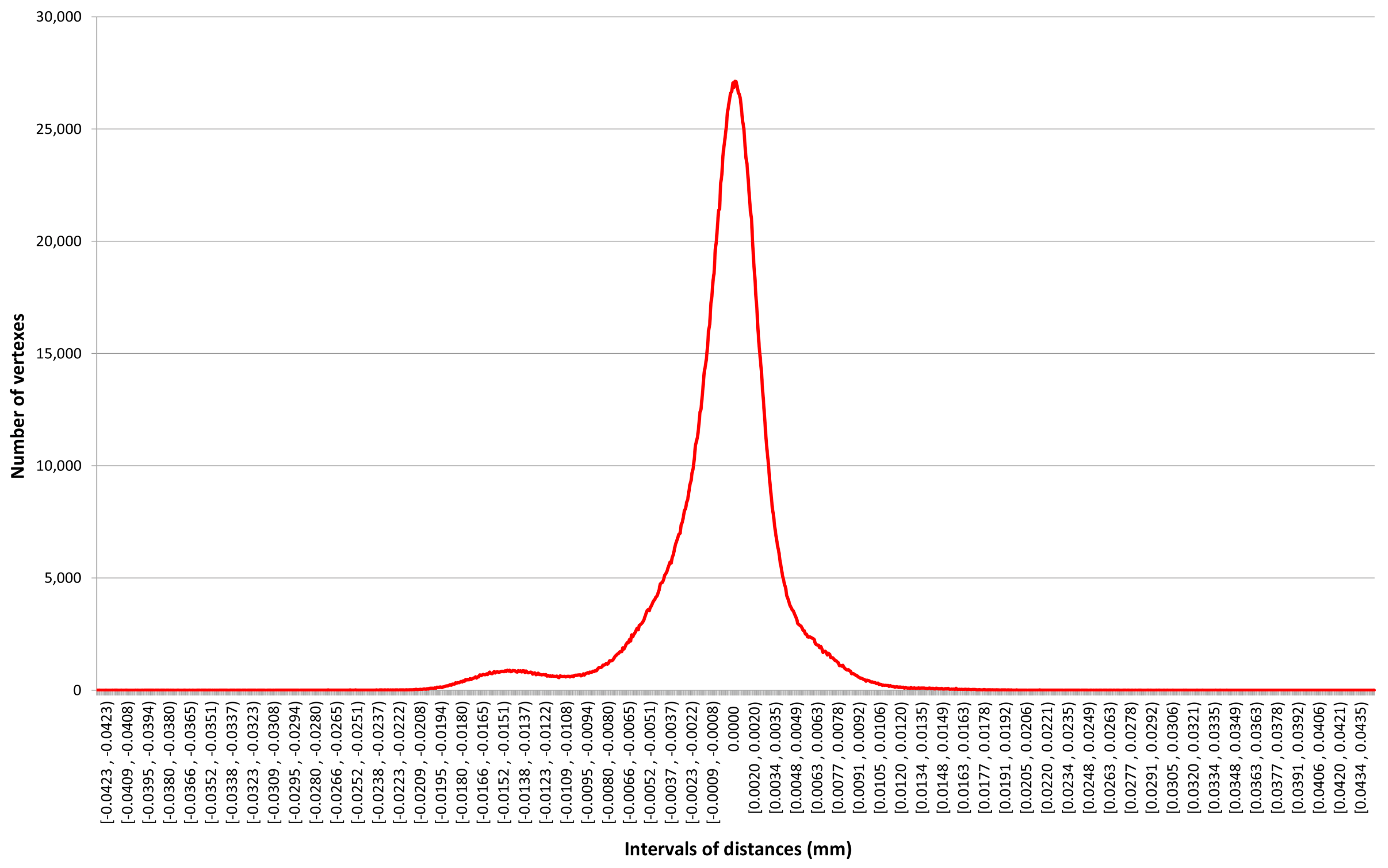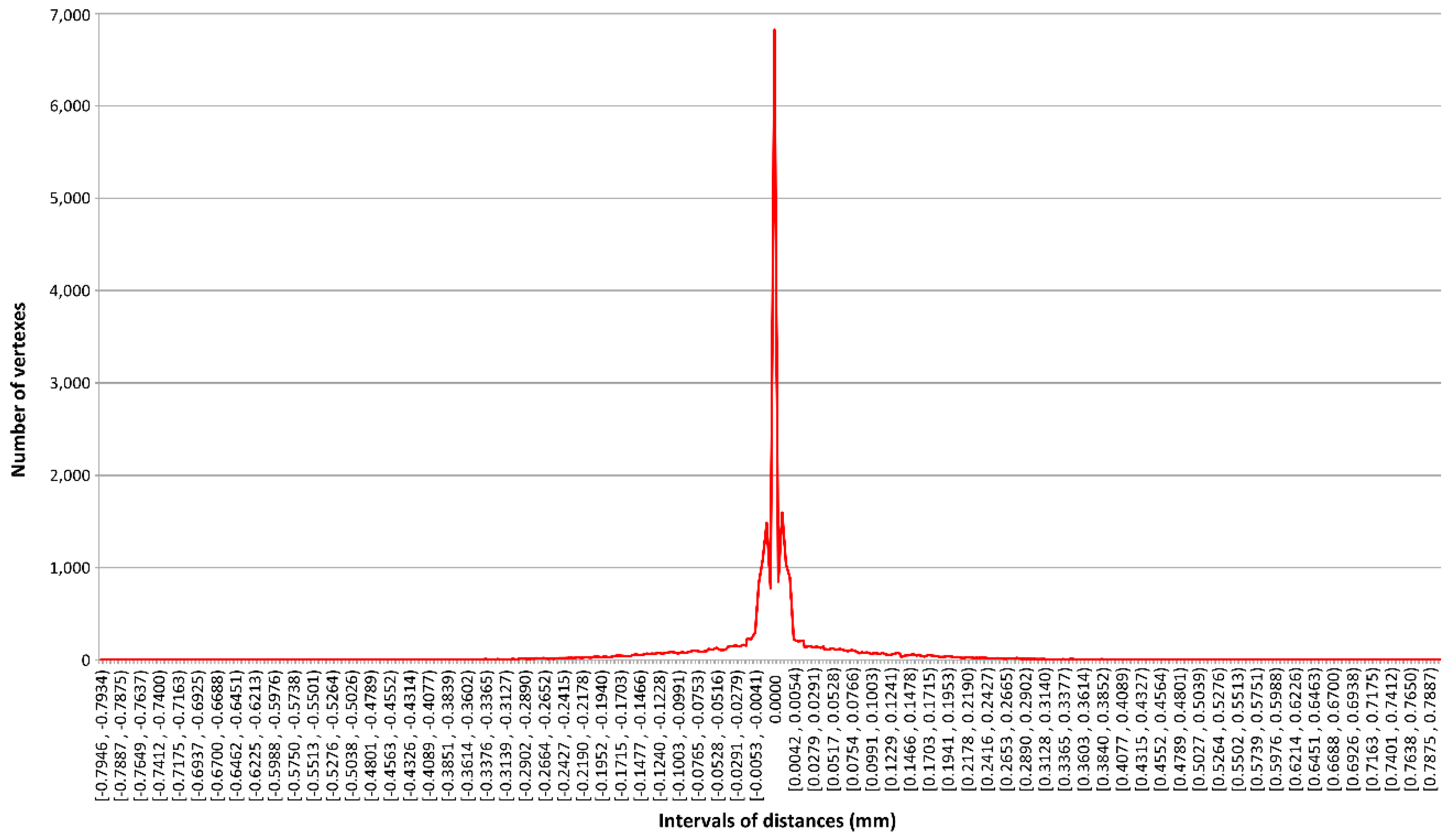This can be observed in Section 5.1, where the difference between the point-cloud-to-mesh (Figure 13) and mesh-to-mesh (Figure 14) deviation graphs is analysed. A greater number of points exist in the intervals surrounding the zero value in the point cloud meshing (mesh 1 from the original point cloud, in Figure 13) than in those of the mesh simplification (mesh 2 from mesh 1, in Figure 14). This could be due to the way the mesh is produced from the reference object—original point cloud or mesh—it is revealed that the smoothening to reduce the number of triangles is not as accurate as the simplification. Therefore, the smoothening level and the simplification degree considered in this research proves to be suitable for the digital reconstitution of the basilica. The simplification of these geometries according to the optimal parameters obtained from the 3D meshing validation test eases the data processing and modelling in comparison with original (non-simplified) complex meshes. In this research, the threshold of 20,000 faces per drum is established, but the minimum triangle quantity achieved in a drum is even higher (29,232 faces in drum 3, column C5). These data are gathered in Table S1 (Supplementary Materials). The geometry accuracy achieved is represented in Table 10 as both the standard deviation of the meshing accuracy and the mesh simplification, and as average triangle surface from all the columns, which is weighted according to the total of triangles in drums per column. As calculated in Table S2 (Supplementary Materials), the total of faces obtained in the basilica is approximately 8 million, the total column surface is 269.688 m² and the total volume is 29.697 m³. From the aforementioned, it is necessary to refer to the work by Korumaz et al. [29], given the fact that they also use TLS for geometry capture, mesh and solid modelling for FEM analysis. In their case, the original and simplified point clouds have 7 and 3 million points, which constitutes a significant reduction in comparison with the dense point cloud of the columns in the basilica of Baelo Claudia (56 million), despite the great dimensions of their case study (minaret). In addition, the Octree depth 12 is suitable for the simplified point cloud data of the minaret, whereas it generates noise in denser point clouds as in the basilica.

Focusing on the physical features of the solid models (see Figure 10) for the column C19, created through the three different modelling approaches, it is worth describing the differences and similarities they involve. Concerning the as-built model, the surface deformations of the drums and their joints become evident: neither the relief is homogeneous, nor the joints are horizontal. The distortion of the drums and the general displacement of the column at the top are also clear. In contrast with Korumaz et al. [29] and most of the research works gathered in Section 2 in this paper of the Baelo Claudia case study, CAD software is not used to create some parts of the columns from documentary sources. Moreover, the geometric analysis in the columns of the basilica provides full measurements of displacements, distortions and deformations on the top view instead of in one axis of tilt. Consequently, the analyses carried out are based on scanned geometry, considering the deformations of the columns surface, which is useful to identify particular geometry alterations for subsequent restoration works.

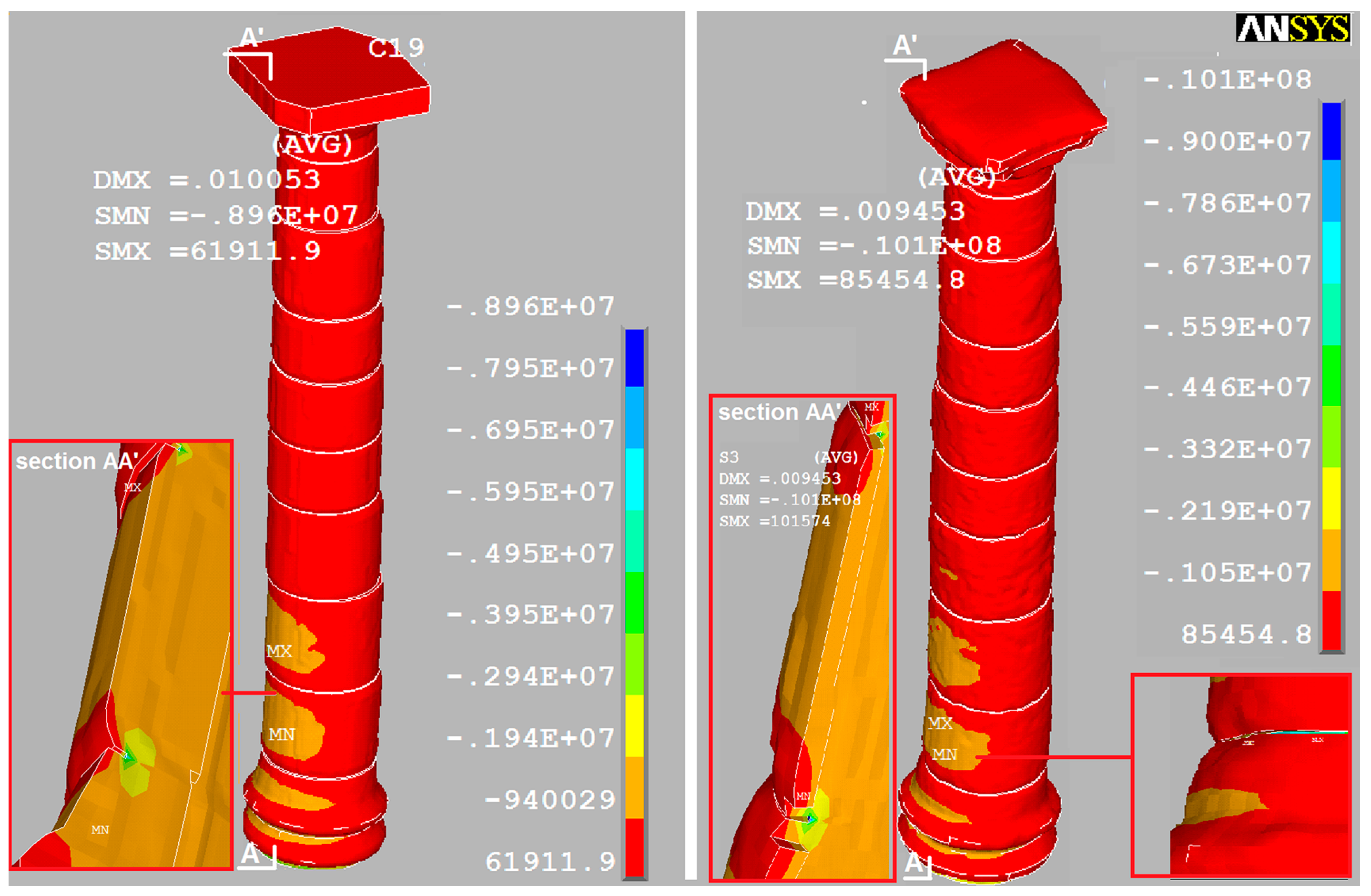
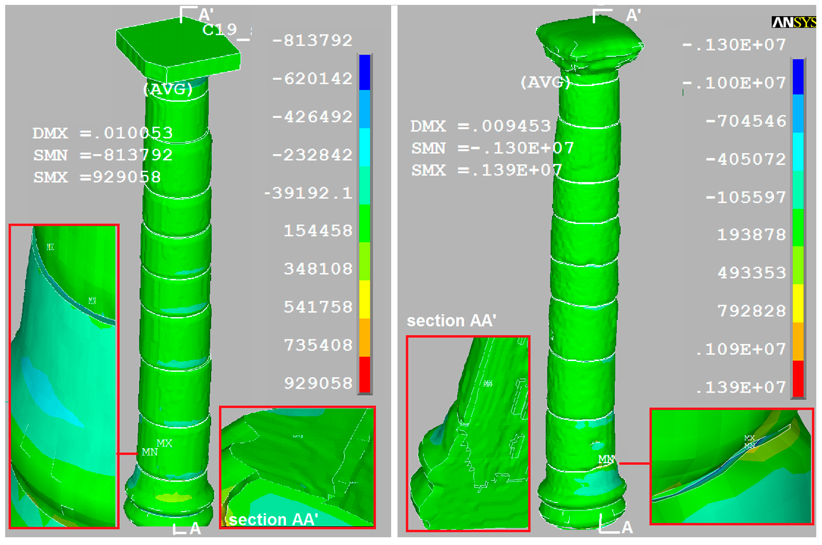
In relation to the structural behaviour assessment, the as-built modelling approach has great impact on the results of the analysis in terms of compliance factor accomplishment—especially when both the axial ultimate limit state and the shear stress field are analysed. The simplified model maintains the distortion and displacement of the drums and the column, respectively, but it avoids the deformation of the drums surface and their joints. Concerning the ideal model, it only considers the average diameter and the actual height of the drums, but using primitive geometries (cylinders); the base centroids remain invariable in relation to the other approaches. The regular geometry of the ideal model, as shown in the structural analysis results, implies minor structural deformations and stresses as well as a significant stress redistribution (especially in the compressive stresses) as expected. As explained in Section 5.3, the differences between the as-built and the simplified model, which reproduce the most realistic geometries, are more significant in the stress field than in the displacement field. Thus, the maximum Sxz shear stress undergoes 50% increase in the as-built model. That could represent the unfulfillment of the shear ultimate limit state under dynamic loading. Additionally, the maximum principal stress S3 exhibit 13% increase when the as-built model is compared to the simplified one. However, as far as the eigenvalue analysis is concerned, the differences among models are no relevant. Indeed, it is worth highlighting that neither the stiffness degradation nor the geometric imperfections yield a period increase. However, the most crucial difference that is provided from the structural assessment is the value of the compliance factor, which is of fundamental interest within structural safety assessment. The axial ultimate limit state compliance factor is accomplished in the ideal and simplified models, but in the as-built model is less than the accepted limit value of 1.0. Those divergent values represent the difference between deciding whether strengthening and/or retrofitting works are necessary or unnecessary.

The as-built modelling allows the accurate measurement of the geometrical alterations and the structural behaviour assessment on the columns in the basilica of Baelo Claudia. The potential of the proposed methods is clear, since their application to different archaeological and architectural heritage assets in the cities would enrich the analyses of their physical status for conservation purposes. The quantitative data to study the displacement, distortions and deformations of the elements, as well as the volume and surface of columns and drums gathered in Table S2, can be used by the specialists to both assess the refurbishment needs in accordance with technical and scientific criteria and conduct health monitoring from changes in their geometry. In addition, the geometric analysis can be implemented for other shapes of archaeological or architectural heritage models from TLS, whether they are based on pure parametric objects (using basic shapes such as circumference, arc, rectangle, etc.) or using closed polysurfaces (solids) from meshes as the as-built models in this paper. In this way, although this research article focuses on the analysis of columns, other element typologies can be geometrically assessed within their reference coordinate system. The analysis of diverse structural components—foundations, walls, beams, rafters, etc.—through, e.g., cross-sections or centroids displacement, and the deformation calculation due to tilt, bulges, deflections, etc., reveal their conservation status.

It is also worth noting that, although this research has not considered specific BIM software yet, the outcomes of this case study (the columns of the basilica of Baelo Claudia and the analysis data obtained) could be considered a HBIM, since the accurate 3D modelling of archaeological heritage sites supported by TLS point cloud data is achieved. According to Azhar [67], BIM goes beyond software; it is considered a process or a methodology rather than the mere use of certain programmes. The as-built models of this paper can be easily transferred as IFC (industry foundation classes) format to interoperate with BIM and later insert data, such as the geometric and FEM analyses results.

Concerning the limitations of this research, the 3D scanning was carried out within a user coordinate system. The global point cloud was not geo-referenced using GNSS due to technical issues during the survey. For this reason, the orientation of the basilica at the geometric analysis stage was established according to the site map provided by Fincker et al. [41]. The model geo-referencing would entail more accuracy in the results of the column leaning orientation. However, from Table 9, the low tilt error achieved is considered valid to calculate the displacements, distortions and deformations of columns and drums and, therefore, suitable for the purpose of this research, which is to rationalise the need of creating as-built models to support analyses more accurate than those performed utilising non-deformed heritage 3D models.

The capture of the joints between drums at a higher position was not possible due to the limitation of the scanning survey itself, since the device is placed on the ground level, surrounding the columns. Consequently, the joints’ geometry was simplified as described in this paper.

In addition, it should be said that the semi-automatic procedure and algorithm to subdivide the columns into different parts entail the manual insertion of points on the drum edges near the joints. Further improvements of this process could consist on the implementation of artificial intelligence (AI) by pattern recognition to set the points, which define the (patch) surfaces to split the columns. The AI could be also implemented for ground removal (point cloud segmentation) to extract the columns.

Other future research works will consist of a thoroughgoing assessment of the available meshing algorithms in terms of accuracy to produce as-built 3D heritage models, since the structural analyses on these assets could benefit from more precise geometries.

7. Conclusions

The results of this research derive from the geometric analysis and the structural behaviour assessment of the as-built models produced by using terrestrial laser scanning, semi-automatic modelling methods and algorithms. The as-built solid models of the columns in the basilica are created in different stages: (1) from TLS with a 0.0385° tilt error and 4 mm point accuracy at 10 m; (2) point cloud 3D meshing with an accuracy of 4,432.06 points (standard deviation in comparison with the original point cloud); (3) mesh simplification degree with an accuracy of 239.84 points (standard deviation in comparison with the original mesh); and (4) an average triangle resolution of 33.28 mm² and the weighted value of 64,037.56 faces per drum, which is higher than the modelling simplification threshold of 20,000 triangles per drum set in this research to achieve accurate geometry in columns.

In order to provide quantitative results from the geometric analysis, the following findings are highlighted:

• Focusing on the global column displacements gathered in Table S1. Displacements and distortions in columns (Supplementary Materials), four out of 11 columns have capital present values above 65 mm, whereas only three have displacements below 20 mm.
• It is revealed the poor conservation status of columns C3, C7, C2, C17, C19 and C20 in terms of structural alterations, the last four having the highest values of both displacement and distortion when compared to the ideal model: their joint mean values are 85.10 mm and 46.97 mm, respectively.
• The global displacement of column C19 is 132% higher than the average displacement (47.26 mm) of the columns with capitals. In relation to C19′s distortions, the value accounting for the vertical ideal axis is 235% greater than the average distortion of all the columns (19.92 mm), and the distortion with respect to the drums below is 80% higher than the mean (9.06 mm). Thus, as seen throughout this paper, C19 is the most unfavourable column and, therefore, constitutes a suitable sample for the structural analysis.

On the other hand, the following conclusions are obtained from the numerical structural assessment:

• The modal results are quite similar among models, and neither the stiffness degradation nor the geometric imperfections (leaning and distortions) provoke a significant period increase. The only difference is that the leaning leads to an effective mass redistribution in the horizontal axis, but maintaining the modal shape nature.
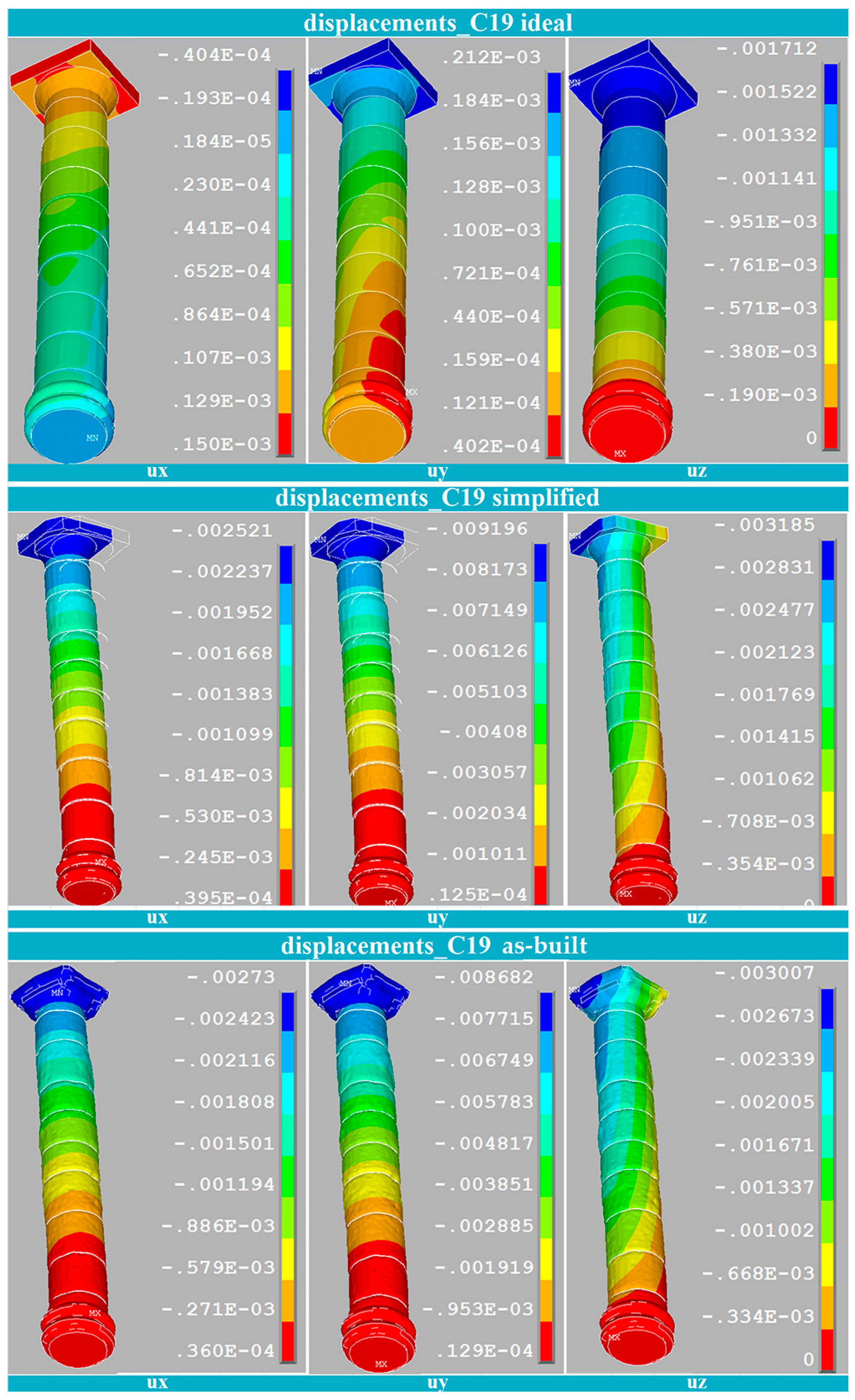
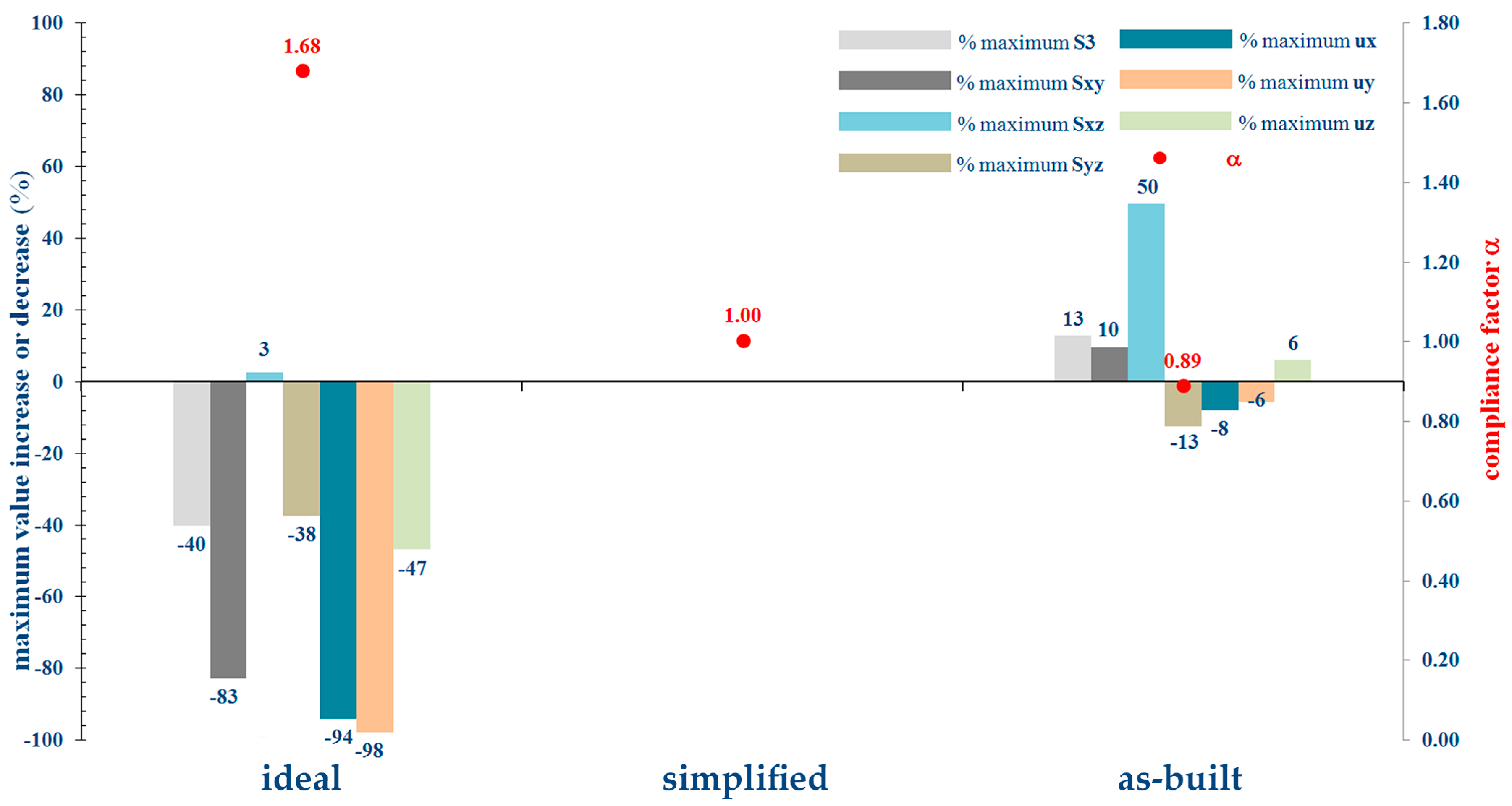
• The maximum displacement and stress values exhibit significant differences among models: (i) In the displacement field, the column tilt provokes relevant variations between the ideal model and the most realistic ones (simplified and as-built), as expected. Taking the simplified one as the reference, the u_y displacement decreases 98% in the ideal model and 6% in the as-built one. (ii) In the stress field, considering the simplified model as the reference, the stresses values present an important decrease in the ideal model (e.g., 40% in the maximum compressive value, S3, and 83% in the shear stress, Sxy). The differences in the shear stress values between the simplified and the as-built models are also remarkable, as the obtained variation (50% increase in the as-built model) could represent the unfulfillment of the shear ultimate limit state under dynamic loading.
• The most important difference is the compliance factor value. The axial ultimate limit state compliance factor is accomplished in the ideal and simplified models (1.68 and 1.00, respectively), but in the as-built is not completely fulfilled (0.89). Those divergences actually make the difference between deciding whether strengthening and/or retrofitting works are necessary or unnecessary. From those results, the necessity of strengthening or retrofitting measures should be clarified on the basis of risk-based decision criteria. In any case, the requirement for an accurate representation of the real geometry when assessing structural performance is demonstrated, as it has been achieved within the methodology proposed in this work.

Therefore, this paper highlights the relevance of modelling the archaeological and architectural heritage accurately from remote sensing. Here, the simulations and geometric analysis become a direct application of the integration of point cloud data into the as-built modelling of heritage. In this sense, the implementation of the methods described into other sites leads to achieve the as-built 3D heritage city modelling in order to contribute to the conservation of these assets for the future.