Characterizing the Variability of the Structure Parameter in the PROSPECT Leaf Optical Properties Model

Abstract

Radiative transfer model (RTM) inversion allows for the quantitative estimation of vegetation biochemical composition from satellite sensor data, but large uncertainties associated with inversion make accurate estimation difficult. The leaf structure parameter (N_s) is one of the largest sources of uncertainty in inversion of the widely used leaf-level PROSPECT model, since it is the only parameter that cannot be directly measured. In this study, we characterize N_s as a function of phenology by collecting an extensive dataset of leaf measurements from samples of three dicotyledon species (hard red wheat, soft white wheat, and upland rice) and one monocotyledon (soy), grown under controlled conditions over two full growth seasons. A total of 230 samples were collected: measured leaf reflectance and transmittance were used to estimate N_s from each sample. These experimental data were used to investigate whether N_s depends on phenological stages (early/mid/late), and/or irrigation regime (irrigation at 85%, 75%, 60% of the initial saturated tray weight, and pre-/post-irrigation). The results, supported by the extensive experimental data set, indicate a significant difference between N_s estimated on monocotyledon and dicotyledon plants, and a significant difference between N_s estimated at different phenological stages. Different irrigation regimes did not result in significant N_s differences for either monocotyledon or dicotyledon plant types. To our knowledge, this study provides the first systematic record of N_s as a function of phenology for common crop species.

1. Introduction

Terrestrial biogeochemical cycles are primarily driven by plant physiological and ecological processes involving the exchange of matter and energy, such as photosynthesis and evapotranspiration [1,2,3]. Knowledge of plant canopy biochemical composition provides critical information towards understanding and predicting the flow of energy and matter within terrestrial biogeochemical cycles [4,5]. However, generalizing field measured plant or canopy biochemical processes, albeit locally accurate, is not a feasible method for inferring larger landscape ecosystem processes.

Spaceborne radiometric remote sensing measurements of solar electromagnetic radiation, reflected by the Earth’s surface, can be used to monitor physical interactions between leaf properties and canopy structure, thereby delivering valuable information relevant to terrestrial biogeochemical cycles [6,7,8]. Empirical methods, which rely on statistical relationships of observed phenomena with remote sensing measurements, are widely applied as being simple and computationally efficient. Typically, with this approach, multispectral reflectances are combined into vegetation indices, designed to maximize the sensitivity to parameters of interest while minimizing the influence of unrelated factors, including soil or atmospheric effects [9,10]. The vegetation indices are subsequently correlated to biochemical variables such as photosynthetically active pigments, water, and biomass.

The systematic application of vegetation indices for quantitative biochemical component estimation, however, is hampered by large uncertainties. Spectral indices are inevitably sensitive to multiple biochemical and structural characteristics of vegetative canopy systems, and are constrained by the representativeness of the training data needed by this approach [11,12,13]. Alternatively, physical-based approaches may be applied to overcome transferability problems that arise during systemic application [14].

Physical-based approaches are used to estimate canopy biochemical and structural characteristics through radiative transfer modeling by simulating the interactions of electromagnetic energy with leaf and canopy surfaces based on the laws of physics [15,16]. Among these, leaf optical spectral properties are critical indicators of plant physiology [17,18,19], which affect other functional processes up to ecosystem levels [3]. Leaves also act as the primary scattering and absorbing elements of plant canopy systems [20,21].

The leaf Propriétés Spectrales radiative transfer model (PROSPECT), which simulates hemispherical reflectance and transmittance of a leaf in reflective wavelengths in the 400–2500 nm spectral region [22], is one of the most widely applied physical-based models for leaf trait estimation [23,24]. The model has been successfully used to estimate leaf biochemical components by inverting leaf reflectance measurements [13,24,25].

PROSPECT is based on the plate theory model [26], where a leaf is conceptualized as one or multiple compact absorbing plates with rough surfaces. The model calculates the radiative transfer of energy at the surface and inside the leaf as a function of: (1) the angle of incidence of incoming radiation α, (2) the refractive index n(λ), (3) a dimensionless leaf structural parameter that represents the number of homogenous layers (or plates) N_s, and airspaces N_s − 1, specifying the number of cell wall/air space interfaces within the plant leaf mesophyll, and (4) the contents of biochemical components per leaf area Cspe, multiplied by the corresponding absorption coefficients k_spe(λ).

Several versions of the model have been published since first introduced in 1990 [12,22,27,28]: the most recent version being PROSPECT-5 [29] and PROSPECT-D [30]. The biochemical components used in PROSPECT-5 are presented in

Table 1. Biochemical parameters used by the PROSPECT-5 model.

Symbol	Biochemical Parameter	Units
Ccab	Leaf chlorophyll content	µg cm−2
Ccar	Leaf carotenoid content	µg cm−2
Cw	Equivalent water thickness	g cm−2
Cm	Dry matter content	g cm−2

.

In the PROSPECT-5 version of the model, the incidence of incoming radiation α, refractive index n(λ), and specific absorption coefficients k_spe(λ) have been estimated and fixed in the model [29]. Therefore, the estimation of a single leaf’s reflectance and transmittance in PROSPECT-5 is driven by user inputs: The N_s parameter and contents of the biochemical components per leaf area C_spe. The spectral absorption coefficient k(λ) is estimated as:

$$k\left(\lambda \right)=\frac{\left(C_{cab}\ast k_{cab}\left(\lambda \right)\right)+\left(C_{car} \ast k_{car}\left(\lambda \right)\right)+\left(C_m\ast k_m\left(\lambda \right)\right)+\left(C_w\ast k_w\left(\lambda \right)\right)}{N_s},$$

(1)

Leaf transmittance τ(λ) and reflectance ρ(λ) are subsequently derived from the spectral absorption coefficient k(λ), angle of incidence of incoming radiation α, refractive index n(λ), and number of airspaces N_s − 1 following the methods introduced by Jacquemoud and Baret [22].

The inversion of a model for the retrieval of biophysical variables is inherently an “ill-posed” problem [31]: in many cases, it is likely that more than one set of values of the variables would satisfy the inversion. Combal et al. [31] recommended the use of a priori information to address the “ill-posed” nature of the problem by constraining the range of biophysical values resulting from the inversion, thereby eliminating unrealistic solutions. Several studies have reported significant improvements to biophysical parameter retrieval by using a priori information to constrain the inversion [32,33,34]. There is still a need, however, to advance our knowledge of the range of key biophysical variables and of associated uncertainties [31,35,36].

The N_s parameter is a major source of uncertainty in the inversion of the PROSPECT model as it is the only parameter that is based on a conceptual quantity (i.e., number of plates) rather than a measurable physiological trait. Theoretically, N_s is connected to leaf characteristics such as thickness and intercellular properties, including fraction of airspace and mesophyll cell structural dimensions [22,37]. The internal structural properties and cell types (i.e., epidermis, palisade, and spongy mesophyll) of leaves play a key role in regulating internal light for maximizing photosynthetic activity, especially with regard to energy not easily absorbed at the leaf surface [38,39]. For example, upper epidermis cell shape (spherical vs elliptical) dictates the distribution of intercepted energy within the leaf while palisade mesophyll cells act as a conduit for photons to enter the spongy mesophyll. Spongy mesophyll cells and interior air spaces (many air–water interfaces) induce a scattering effect to maximize absorption by chloroplasts. Since the visible (400–750 nm) and mid-infrared (> 1400 nm) regions are governed by the two primary absorbers in leaf tissue (pigments and water, respectively), the NIR wavelengths (750–1400 nm) represents the region in which leaves are most optically transparent and is primarily influenced by leaf structural properties [40]. In PROSPECT, these intercellular characteristics are lumped into the N_s parameter. Previous approaches to link N_s with physical traits, like specific leaf area (SLA), are based on empirical relationships that are difficult to transfer [41]. As a result of the simplification of leaf structural properties, N_s cannot be easily connected to any corresponding physical traits [40].

The sensitivity analysis conducted by Ceccato et al. [41] demonstrated that N_s is a key parameter within PROSPECT. When applying the model in direct mode to estimate leaf reflectance at 1600 nm, N_s has the greatest influence on the uncertainty of the model output (41.1%), as compared to leaf water content (36.4%) and dry matter content (22.5%). Consequently, when applying the model in inverse mode, constraining the range of possible N_s values would greatly reduce the uncertainty in estimating other biophysical variables of interest.

Jacquemoud and Baret [22] indicated that the different structural properties of monocotyledon and dicotyledon species cause differences in estimated N_s values, with monocotyledon leaves ranging between 1 and 1.5 and the thicker and structurally more complex leaves of dicotyledon leaves resulting in N_s values between 1.5 and 2.5. Processes driven by leaf growth are also important when considering the scattering of energy. Demarez [42] observed seasonal variation of N_s in select temperate deciduous forest species and linked the change of N_s throughout time to the development of the leaves. In that study, N_s increased gradually during leaf tissue development in the initial growth stages, plateaued during most of the summer months, then rapidly increased during senescence. The rapid increase of N_s at the end of the study period was linked with an amplified scattering effect caused from degradation of leaf structural features resulting from the reduction of leaf water content. This link was made because, as leaves approach fully turgid or wilted states, leaf cell size, shape, and distribution are altered resulting in changes in scattering properties [43]. Despite this, we are not aware of any studies that examine the effect of water stress on N_s, regardless of the fact that several studies used PROSPECT inversion to estimate vegetation water content [41,44,45,46,47].

A few studies exist that examine the variation of N_s as a function of vegetation physiological status (i.e., water stress) and phenology [13,22,27,42], but no prior study presents a comprehensive analysis of this relationship. Zhang et al. [13] established an indirect relationship between leaf reflectance and copper stress through the N_s parameter in two crop species at two vegetative growth stages. Jacquemoud and Baret [22] used a limited set of greenhouse measurements to state that a difference exists between estimated N_s in monocotyledon and dicotyledon leaves; Jacquemoud et al. [27] found that this difference might not be observed on leaves grown outdoors, but neither study took phenology into consideration. Finally, Demarez [42] reported estimated N_s from leaves at various stages throughout leaf development, but this study was limited to temperate tree species grown in a deciduous forest under the same environmental conditions. Furthermore, to the best of our knowledge, no published dataset reports reference N_s values of common monocotyledon and dicotyledon crop species throughout the growing season.

The present study is designed to assess whether there is a statistically significant variation in N_s as a function of phenology and irrigation, and to provide reference values of N_s to be used as a priori information for the inversion of PROSPECT in future research.

The present study involved three main components: (1) a large data collection experiment was performed over two growing seasons to collect a comprehensive dataset of leaf optical spectral measurements for use in N_s estimation; (2) PROSPECT-5 was inverted to estimate N_s using the leaf optical spectral dataset; (3) the distribution of estimated N_s values was analyzed statistically as a function of phenological class and irrigation regime.

2. Materials and Methods

2.1. Data Collection

An extensive experiment was conducted in which plants (monocotyledon and dicotyledon) were grown under controlled conditions to collect a representative dataset of leaf optical spectral measurements over a period of 90 days, to cover the full phenological cycle of the plants. Additionally, the plants were subjected to different irrigation regimes to create controlled water stress conditions. Measurements were performed throughout the entire growing season. The phenological stages of the plants grown were aggregated into three main phenological classes, defined to delimit periods in which plants are most temperature and water sensitive.

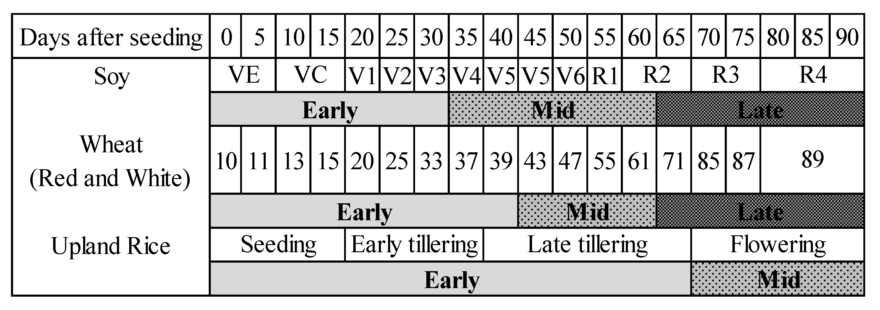
2.1.1. Experimental Design

Pitkin’s forest research nursery during the summers of 2015 and 2016 contained three monocotyledons (hard red wheat—Triticum durum Desf., soft white wheat—Triticum aestivum L., and upland rice—Oryza sativa L.) and one dicotyledon (soy—Glycine max L.). All four were grown in 2015, and two were also grown in 2016 (hard red wheat and soy). The plants were grown outdoors in 45-well foam trays. Watering was controlled, following the procedures detailed below. Other environmental variables, such as temperature, sunlight, and exposure to wind were not controlled.

Each tray contained 45 plants of the same species (one plant for each well); 2–3 seeds per well were initially planted. After plant emergence, if more than one seed had germinated in the same well, the additional plants were removed to ensure one seedling per well. Plants were watered through sub-irrigation methods, allowing for direct control over the amount of water administered while limiting tissue disease. The water for sub-irrigation contained a mixture of starter fertilizer to obtain a nitrogen content of 50 ppm. To water a tray, an 18-gallon bin was filled with approximately 3 gallons of the nitrogen starter mixture. The tray was placed in the bin to allow the starter mixture to soak the tray up from the bottom. The tray would remain in the starter mixture for 30 minutes before being removed. To determine whether sub-irrigation was necessary, each tray was weighed every day. The tray was irrigated only if on that day its weight had dropped below a given percentage of the initial tray saturation weight.

Plant extraction for performing the measurements began approximately 27 days after planting to allow the plants to establish. For the plants grown in 2015, plant extraction and leaf optical measurements occurred regularly once a week and three plants were removed from each tray during the extraction. In 2016, plant extraction and measurements were dependent on watering frequency. Two plants were extracted and sampled immediately before watering occurred and again 24 h after watering occurred.

The life cycle stages of the plants were aggregated into three main phenological classes (early, mid, late), reported in Figure 1.

These three phenological classes were defined based on the sensitivity to drought (water deficit) and temperature of each growth stage for each crop. The ‘early’ class was defined to include the vegetative periods, where extreme temperatures and water deficit have consequences that slow or stop development and reduce yield in later life cycle stages [51]. The ‘mid’ and ‘late’ classes encompass the flowering and yield formation phases of the crop’s life cycle, respectively. In terms of successful yield, these periods are the most sensitive to water and temperature extremes [51]. The crops used in this study are less susceptible to drought or extreme temperatures when full maturity is achieved. Therefore, life cycle stages after the ‘late’ phenological class were not considered, and plants were no longer sampled.

Since the plants were grown outdoors, the samples were subjected to the same temperature and sunlight conditions. The upland rice plants did not grow past the flowering growth stages as the local outdoor conditions slowed development in the early and mid-phenological classes. As the experiment ended after 90 days, before the upland rice plants reached the ripening growth phase, the upland rice samples were aggregated into two phenological classes only (early and mid).

In 2015, plants were separated into three separate irrigation regimes resulting in three groups of four trays (four species)—for a total of 12 trays. The trays were weighed daily at approximately the same time of day to determine if watering should occur. Irrigation occurred when the tray reached 85%, 75%, and 60% of the initial saturated weight measured at the beginning of the growing season for regimes 1, 2, and 3, respectively.

In 2016, all plants were watered following the same regime, hence only one tray per species was grown. As in the 2015 experiment, the trays were weighed daily at approximately the same time of day to determine if irrigation would occur. Irrigation occurred when the tray reached 60% of the initial saturated weight measured at the beginning of the growing season.

2.1.2. Measurement Protocol

Extraction occurred by cutting the plant at the base, just above the soil line, and immediately placing it in a plastic bag to minimize water loss. Bags were put in a cooler until processing in the lab approximately an hour after extraction. Leaf sample water loss was assumed to be minimal during transportation to the lab for measurements. Extraction and leaf measurements occurred at approximately the same time each day.

Leaf bidirectional reflectance factor (ρ_BRFλ) [dimensionless] and transflectance [dimensionless] were measured with a PSR-3500 field spectroradiometer (Spectral Evolution, Inc). The instrument collects measurements on a full spectral range of wavelengths, from 350 nm to 2500 nm, with a spectral resolution of 3 nm at 700 nm, 8 nm at 1500 nm, and 6 nm at 2100 nm. All data were interpolated to 1 nm sampling interval before further processing, resulting in 2151 bands. The field spectroradiometer was equipped with a pistol-grip contact probe with leaf clip, using a 5-watt tungsten halogen source at 12-degree incidence zenith to the target for spectral measurements. The leaf clip attachment for the contact probe includes a two-sided reversible plate that holds the leaf sample during measurement and excludes ambient direct and scattered light from the sensor. One side of the plate is a near 100% reflective Lambertian Spectralon panel (Labsphere Inc., North Sutton, NH) and the opposite side is a black surface with near 0% reflectance. Radiance measurements were calibrated using the Spectralon panel before scanning each leaf. The instrument was set to acquire and average 10 spectra per scan to reduce noise and was considered the optimal compromise between time required for spectra collection and noise reduction. Measurements were performed on five points of the leaf and subsequently averaged. The black plate was used to measure ρ_BRFλ as it ensures that only electromagnetic radiation directly reflected by the leaf is measured by the sensor, as any radiation transmitted through the leaf is absorbed by the plate. The white plate was used as the background to measure leaf transflectance, defined as the sum of leaf reflectance and double transmittance: The spectroradiometer acquires the energy directly reflected by the leaf, plus the energy that is transmitted through the leaf, reflected by the Spectralon panel, and transmitted through the leaf a second time [52]. While leaves from all plants sampled after the 27-day establishment period were measured with the leaf clip, only leaves that fully covered the leaf clip field of view area were considered in the present study.

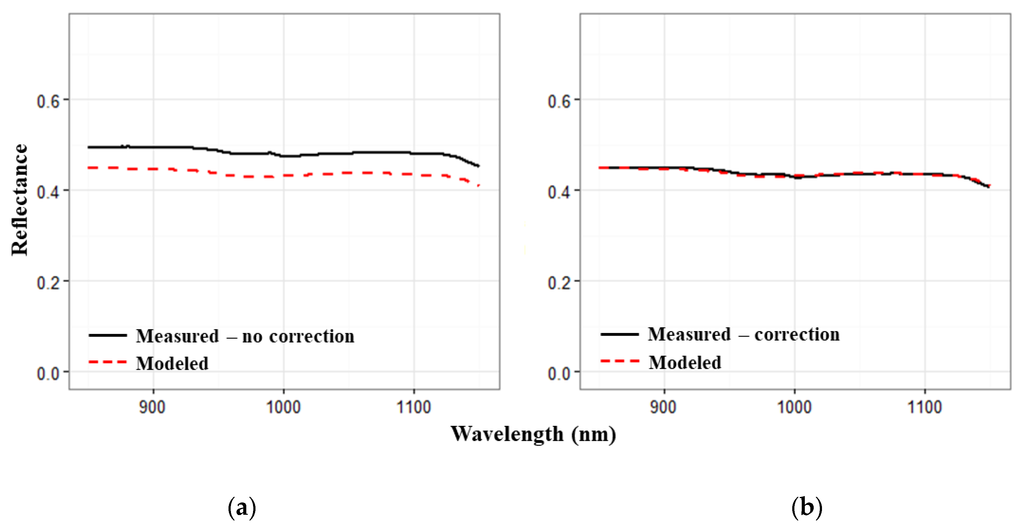
2.1.3. Spectral Data Processing

A function based on the Kubelka-Munk theory of light scattering and absorption was applied to measured leaf transflectance to estimate leaf transmittance (τ_λ) [dimensionless]:

$${\tau }_{\lambda }=\sqrt{\left({\rho }_{TF\lambda }-{\rho }_{BRF\lambda }\right)(\frac{1}{{\rho }_{w\lambda }}-{\rho }_{BRF\lambda })},$$

(2)

where ${\tau }_{\lambda }$ is the estimated transmittance, ${\rho }_{TF\lambda }$ is the measured transflectance of the leaf using the white plate background, ${\rho }_{BRF\lambda }$ is the measured reflectance of the leaf using the black plate background, and ${\rho }_{w\lambda }$ is the measured reflectance of the white plate. Transmittance estimated from Equation (2) has been used in PROSPECT inversion problems with success in previous research [53] and is used in the estimation of N_s for this study due to the unavailability of an integrating sphere for collecting the spectral measurements.

Since the PROSPECT models were originally calibrated on directional hemispherical reflectance spectra (ρ_DHRFλ) measured with an integrating sphere [22,29], inverting the PROSPECT-5 model using leaf clip ρ_BRFλ measurements would not be appropriate [54].

Both ρ_BRFλ and ρ_DHRFλ result from the combination of a leaf surface reflectance component, which accounts for the electromagnetic radiation that does not penetrate the leaf and is directly reflected, and a diffuse reflectance component, which is the result of intercellular physical and biochemical constituents [55]. By separating surface reflectance from the diffuse reflectance, it is possible to correct, prior to the radiative transfer model (RTM) inversion, ρ_BRFλ measured with a leaf clip [56]. Bousquet et al. [55] and Jay et al. [54] summarized and demonstrated the principles, which connect integrating sphere measured ρ_DHRFλ and leaf clip measured ρ_BRFλ, assuming a small incidence zenith, resulting in the characterization of the surface component, which can be used to account for the differences in physical properties between ρ_DHRFλ and ρ_BRFλ:

$${\rho }_{BRF\lambda } -{\rho }_{BRFsur\lambda }={\rho }_{DHRF\lambda } -{\rho }_{DHRFsur\lambda },$$

(3)

At a wavelength of 445 nm, where strong absorption of leaf pigments occurs, it is possible to assume only direct reflectance to occur at the leaf surface [57], thus estimating a simple function, known as PROREF [56], is used to correct the ρ_BRFλ measurement of each leaf sample:

$${\rho }_{meas\lambda }^{\prime }={\rho }_{BRF\lambda } -({\rho }_{BRF445}-{\rho }_{mod445}),$$

(4)

where ${\rho }_{meas\lambda }^{\prime }$ is the adjusted spectral reflectance, and ρ_BRF445, and ρ_mod445 are the measured and modeled leaf reflectance at 445 nm. ρ_mod445 was generated and Equation (4) was computed with each iteration of the N_s inversion step described in Section 2.2, with constant values set for Cc_ab and Cc_ar at 47.28 µg cm⁻² and 10.31 µg cm⁻², respectively, and the N_s value from the iteration. The solution to Equation (5) was computed with each iteration of N_s inversion until minimization was reached. The method for minimization is described in more detail in Section 2.2.

The pigment parameter values were determined by taking the average of Cc_ab and Cc_ar from all of the leaves in the LOPEX leaf dataset [58]. Using only pigment values from soybean and rice leaf, LOPEX samples did not significantly change ρ_mod445 (less than a tenth of a percent). Similarly, the difference in ρ_mod445 generated with N_s = 1 and N_s = 3 was less than a half percent. An example of the PROREF function being applied in the NIR region of measured mature soy leaf spectra is presented in Figure 2.

2.2. Data Analysis

The PROSPECT-5 model was inverted to estimate N_s for each leaf sample, using the three-wavelength inversion method proposed by Féret et al. [29]. The method uses reflectance and transmittances measured at three wavelengths in the NIR plateau, where the leaf spectral response is more sensitive to the N_s parameter, rather than to the concentration of the biochemical components. The three wavelengths are identified based on the measured reflectance and transmittance of each leaf sample in the 800–1300 nm range, as:

• λ₁: Wavelength of minimum absorbance (i.e., the maximum of the sum of measured transmittance and reflectance).
• λ₂: Wavelength of maximum measured reflectance.
• λ₃: Wavelength of maximum measured transmittance.

The approximate location of these three wavelengths are illustrated in Figure 3 on the same example spectra as Figure 2.

The inversion is performed by minimizing a merit function, defined as:

$$J\left(N_s,k_i\left({\lambda }_i\right)\right)= {{\displaystyle \sum }}_{i=1}^3{({\rho }_{mes}\left({\lambda }_i\right)-{\rho }_{mod}\left(N_s,k\left({\lambda }_i\right)\right))}^2+{({\tau }_{mes}\left({\lambda }_i\right)-{\tau }_{mod}\left(N_s,k\left({\lambda }_i\right)\right))}^2,$$

(5)

where λ_i = (λ₁, λ₂, λ₃) are the three wavelengths defined above, ρ_mes (λ_i) and τ_mes (λ_i) are the measured reflectance and transmittance, ρ_mod (λ_i) and τ_mod (λ_i) are the reflectance and transmittance simulated by applying the model in forward mode, and k(λ_i) is the absorption coefficient of an elementary layer N_s at the three wavelengths. The function J was minimized using the Nelder-Mead downhill simplex method [59], setting an arbitrary starting value for the numerator of Equation (1) and N_s, and iteratively searching in the parameter space for the solution resulting in the minimum difference between modeled and measured leaf spectra.

The population of N_s resulting from inversion of the measurements of each leaf sample was analyzed through an ANOVA test to determine whether the range of variation of N_s can be explained by considering plant type (monocotyledon vs. dicotyledon), phenological class (early/mid/late), and irrigation regime (irrigation at 85%, 75%, and 60% of the initial saturated weight, and pre-/post-irrigation). The statistical analysis was conducted as follows:

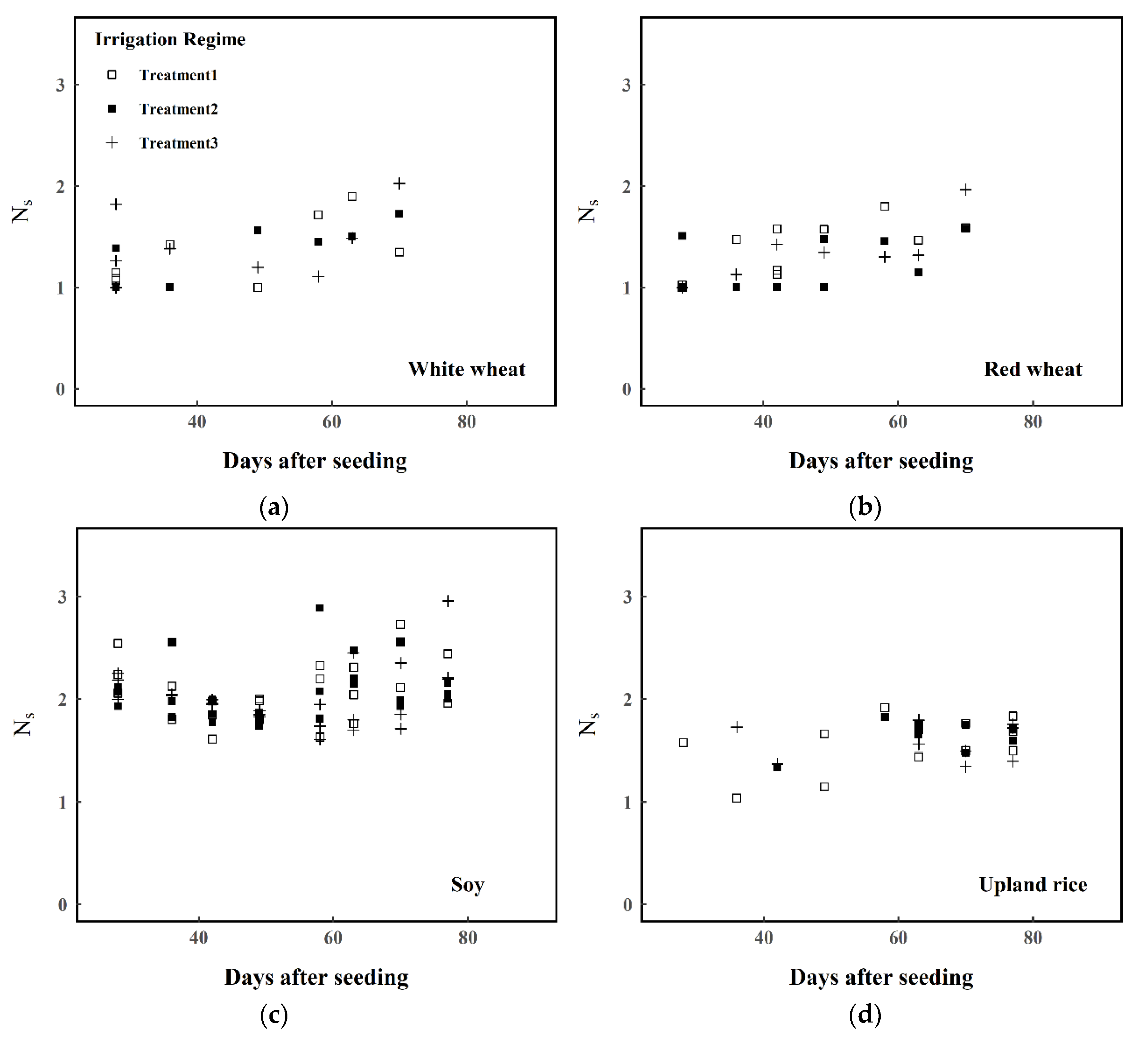
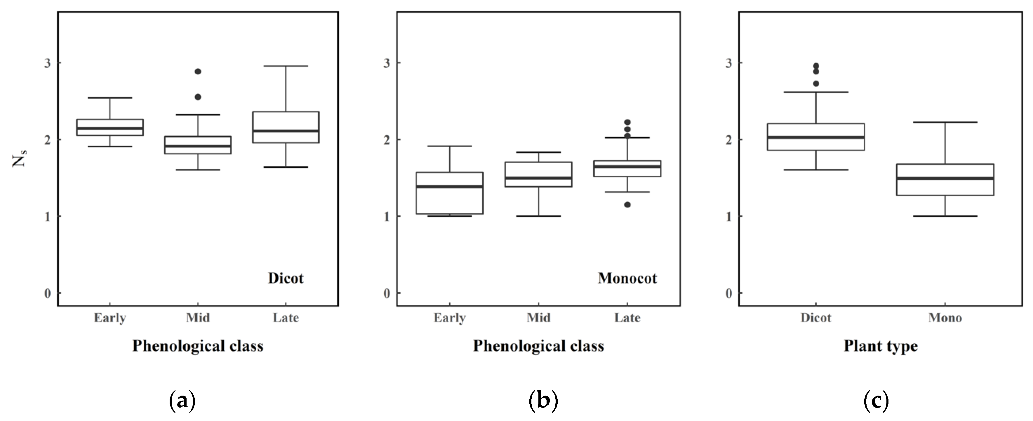
• The population of estimated N_s values was stratified into sub-populations according to the criteria defined in Section 2.1.
• A Welch’s two-sample t-test was performed to determine if the estimated means of monocotyledon and dicotyledon N_s differed significantly from one another.
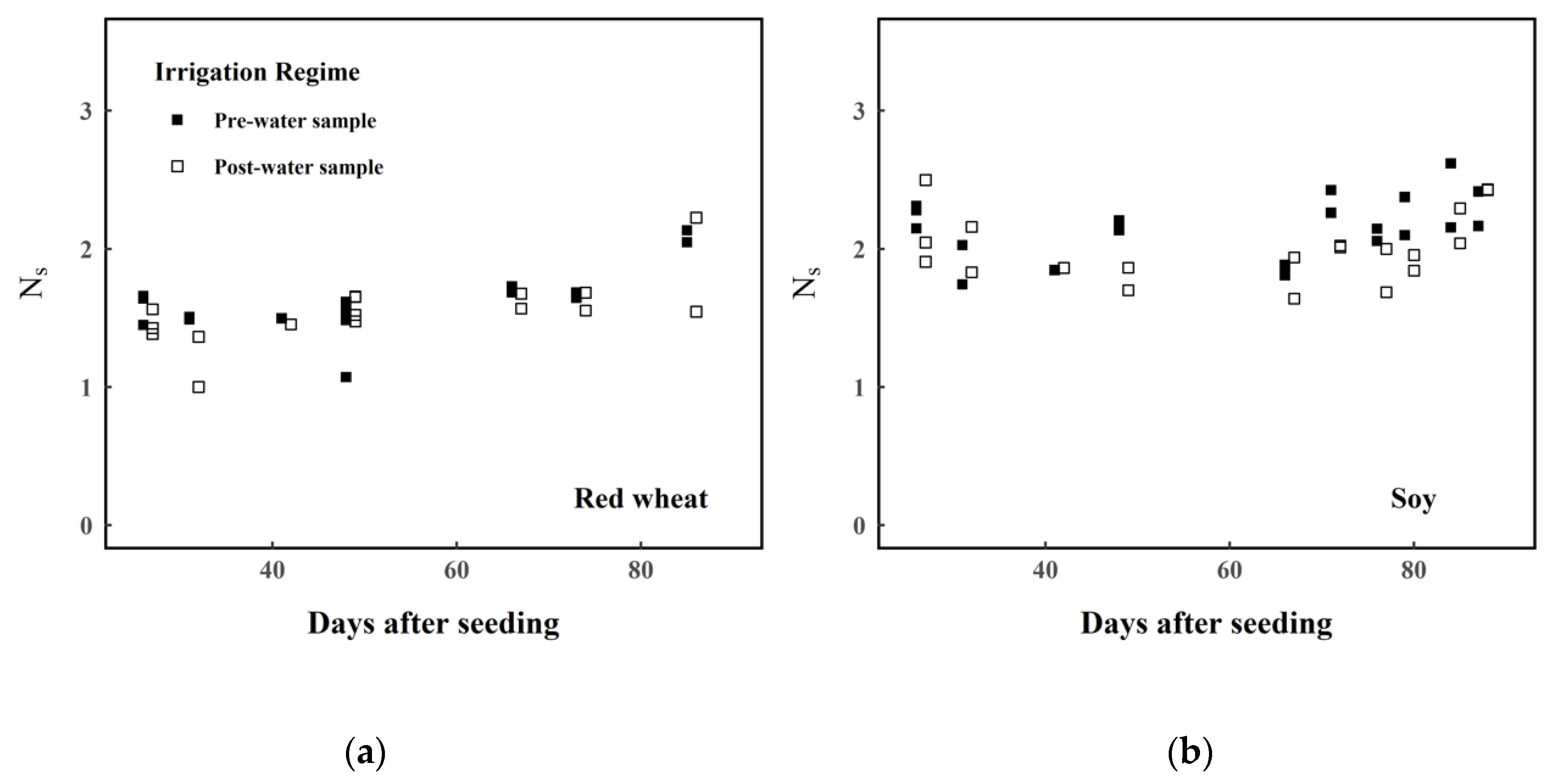
• A Welch’s two-sample t-test was run to determine whether there was a significant difference between the estimated means of pre- and post-irrigation N_s for each plant type.
• Welch’s one-way ANOVA tests were run to test whether the variation of N_s in each plant type can be explained by phenological class (early/mid/late) and irrigation regime (irrigation at 85%, 75%, and 60% of the initial saturated weight)
• If the ANOVA test was significant at P ≤ 0.05, then Welch’s two-sample t-tests were carried out to compare the means of classes within the sub-population of the plant type. For example, if phenological class returned a significant result as an explanatory variable for N_s in the sampled monocotyledon leaves, then the means of ‘early’, ‘mid’, and ‘late’ monocotyledon N_s would be compared.

3. Results

In total, 230 independent estimates of N_s were retrieved from the spectral measurements: 158 from the 2015 experiment and 72 from the 2016 experiment. The timeseries of estimated N_s from the 2015 and 2016 nursery experiments are presented in Figure 4 and Figure 5, respectively. A summary of the estimated N_s, stratified by plant type and phenological class, is presented in

Table 2. Summary of leaf structure parameter (N_s) metrics ¹.

Plant Type	Total	Early	Mid	Late
Monocotyledon (n = 118)
µ	1.46	1.35	1.5	1.66
σ	0.29	0.28	0.23	0.25
Max/Min	2.23/1.00	1.92/1.00	1.84/1.00	2.23/1.15
Upper/Lower IQ	1.68/1.27	1.57/1.03	1.70/1.39	1.73/1.52
Dicotyledon (n = 112)
µ	2.07	2.17	1.96	2.14
σ	0.27	0.19	0.25	0.29
Max/Min	2.96/1.61	2.54/1.91	2.89/1.61	2.96/1.64
Upper/Lower IQ	2.21/1.86	2.26/2.05	2.04/1.81	2.36/1.96

¹ Stratified by species and phenological class. The 75th and 25th percentiles are the upper and lower interquartile (IQ) limits, respectively.

.

The summary in Table 2 illustrates monocotyledon N_s values primarily fit within the range 1.3–1.7 (µ = 1.46, σ = 0.29) and dicotyledon N_s values exhibited a distribution primarily between 1.9 and 2.2 (µ = 2.07, σ = 0.27). Overall, a pattern of N_s increasing with days after seeding was observed with the sampled monocotyledon plants, with lower values in the ‘early’ stage (µ =1.35, σ = 0.28) and higher values in the ‘mid’ and ‘late’ stages: (µ = 1.50, σ = 0.23) and (µ = 1.66, σ = 0.25), respectively. Soy began with higher estimated values of N_s (µ = 2.17, σ = 0.19), lower ‘mid’ stage (µ = 1.96, σ = 0.25), and finally increased during the ‘late’ stage (µ = 2.14, σ = 0.29). The progression of distributions for each plant type over time is illustrated in the box plots of Figure 6, again illustrating the high-low-high pattern for dicotyledon soy and increase over time for the monocotyledon plants. The results from statistical analyses described in Section 2.2 are presented in

Table 3. Welch’s two-sample t-test and analysis of variance ¹.

Data	Independent Variable	F-Value	T-Statistic
All	Species		10.93 (< 0.001)
Monocotyledon	Season period	10.227 (< 0.001)
	2015 Irrigation regime	0.896 (0.413)
	2016 Irrigation regime		−1.122 (0.271)
Dicotyledon	Season period	4.46 (0.017)
	2015 Irrigation regime	2.422 (0.101)
	2016 Irrigation regime		−1.251 (0.22)

¹ Welch’s two-sample t-test and analysis of variance for species, phenological class, and irrigation regime sub-populations. ANOVA results are presented in the first two columns after the independent variable column. Two-sample t-test results are presented in the last two columns. The independent variable name is asterisked if the difference between population means are significant (P < 0.05).

.

The Welch’s two-sample t-test run for the whole dataset (‘all’) comparing N_s means by plant type shows a significant difference (P < 0.001) between the means of monocotyledon and dicotyledon. It was also determined that phenological classes influence the variation of estimated N_s within each plant type, with F(2,115) = 13.40, P < 0.001 for monocotyledon phenological classes and F(2,109) = 7.10, P = 0.001 for dicotyledon phenological classes. Finally, no significant differences were observed between the irrigation regime N_s means for either 2015 or 2016.

Since it was determined that phenological classes were a significant source of variance in estimated N_s, Welch’s two-sample t-tests were run to intercompare the phenological classes sub-population means of N_s (early/mid/late) within each plant type. The results from those analyses are presented in

Table 4. Welch’s two-sample t-test ¹.

Population	Independent Variable	T-Value	df	Probability of > T
Monocotyledon	Early vs Mid	−2.486	88	0.015
	Mid vs Late	−2.626	58	0.011
	Early vs Late	−4.912	84	<0.001
Dicotyledon	Early vs Mid	3.002	59	0.004
	Mid vs Late	−3.3	95	0.001
	Early vs Late	0.373	64	0.71

¹ Results from Welch’s two-sample t-test. The independent variable name is asterisked if the difference between population means are significant (P < 0.05).

. Significant differences between sub-population means of N_s in every consecutive phenological class were observed.

4. Discussion

Our analysis relied on an extensive experimental dataset, collected over two growing seasons with a rigorous data collection protocol. The distribution of estimated N_s was consistent with expected values for monocotyledon and dicotyledon plant types: monocotyledon N_s primarily ranged between values of 1.0–1.5, and dicotyledon N_s primarily ranged between values of 1.5 and 2.5 [27]. The statistical analysis performed on the population of estimated N_s indicated that there was a significant difference between plant types, and that there was a significant difference by broad phenological class. There was instead no significant difference between N_s estimated from plants subject to different irrigation regimes.

The results align with previous literature reporting that structural changes, driven by growth and maturation, influence N_s [23,42]. In particular, we observed a pronounced increase of N_s over time in monocotyledon leaves and a less pronounced dicotyledon seasonality, with higher N_s in the early and late phases, than in the mid growing phase. While the monocotyledon seasonality is in line with previous results derived from measurements on broadleaved plants [42], to the best of our knowledge, the reduced sensitivity of N_s to phenology in certain dicotyledon leaves has not been reported in the available literature. Higher mean N_s in the ‘early’ phenological stages of the dicotyledon plants may be attributed to a change of leaf properties as the leaves begin to mature, i.e., leaf thickness decreasing or the wider spatial distribution of trichomes per unit leaf area as the leaves mature, which affect the transmission of NIR energy. A more detailed investigation of N_s as a function of phenology in dicotyledon species, which will examine a wider variety of species, will be conducted in the future. For monocotyledon N_s, while samples were rejected if the leaf material did not cover the full leaf clip field of view, the strong variation in data points derived from measurements performed less than 60 days after seeding may be attributed to errors with the leaves sampled during the early tillering stages, when in some cases the leaves were still too small for a reliable spectral measurement.

The irrigation regime did not explain the variation estimated N_s. The presence of water either has a direct influence on the spectral signal of leaves, through the rotation-vibration features of water in the mid-infrared region, or an indirect influence, through the structural and physiological biochemical responses of leaves to hydration or dehydration. The result that irrigation regime did not influence the estimation of N_s is consistent with the fact that the estimation of N_s is independent of both direct (i.e., mid-infrared absorption characteristics of water) and most indirect (i.e., changing pigment content) water content influences. Leaf wilting does influence the estimation of N_s, but only when water loss has developed sufficiently enough to result in severe leaf dehydration, causing a significant response in the NIR spectral region [60]. Although the irrigation regime did not have a significant influence over the variance of the N_s parameter in our study, water still has the potential to affect the structural components of leaves and should be considered on an individual species and ecosystem basis along with other environmental factors, such as toxicity, nutrient availability, and disease. Future studies, which examine the influence of wilting or fully turgid cellular properties on the estimation of N_s in more extreme cases, will need to account for irrigation regimes on an individual species basis. Notwithstanding these limitations, the finding that the irrigation regimes used in the current study do not significantly influence N_s has particular relevance as it implies that a priori N_s values, tabulated solely as a function of plant type and phenology (i.e., Table 2), can be used to constrain the inversion of PROSPECT. A common use of PROSPECT is the estimation of canopy water content, and in such case the leaf water content is evidently unavailable to inform the a priori selection of N_s.

A few caveats should be considered if using a priori N_s values, estimated in this study through leaf-level inversions, for canopy level studies. First, the heterogeneity of the canopy should be considered, as different plant types and different phenological stages might be present. Second, N_s may vary within a single species depending on other factors besides phenology, such as environmental conditions [13] and illumination (sun vs shade) [42]. Future research will be focused on coupled radiative transfer model inversion for estimating canopy traits in an agricultural setting where species, environmental conditions, illumination, and phenology are relatively uniform, and on the evaluation of the reduction of canopy water content uncertainty that can be attained by constraining the range of variation of N_s.

5. Conclusions

This paper presents the results of an extensive experiment aimed at the assessment of the PROSPECT radiative transfer model leaf parameter (N_s) as a function of phenological class, and whether water content would indirectly influence the estimation of the N_s parameter. While several datasets of leaf spectral and biophysical properties are available [29,58,61,62], our results, obtained over the full extent of the growing season and accounting for a range of irrigation regimes, provide the first detailed phenology dependent record of N_s values for two common crop species. The results indicate a significant difference between N_s estimated on the considered monocotyledon and dicotyledon plants, and new findings of a significant difference between N_s estimated at different phenological stages. The results also indicate other new findings, namely that irrigation regimes did not result in significant N_s differences for either monocotyledon or dicotyledon plant types. Since only four plant species (three monocotyledons and one dicotyledon) were considered in this study, further research will be needed to assess whether these results can be generalized to different species. A second priority for future research will be on the quantitative assessment of the reduction of uncertainty in estimating plant biophysical variables when applying a priori N_s values in PROSPECT inversions and whether constraining the range of variation of N_s can reduce the uncertainty of retrieving certain canopy variables in coupled radiative transfer model inversion.

References

1. Bonan, G.B. Forests and climate change: Forcings, feedbacks, and the climate benefits of forests. Science 2008, 320, 1444–1449. [Google Scholar] [CrossRef]
2. Running, S.W.; Coughlan, J.C. A general model of forest ecosystem processes for regional applications I. Hydrologic balance, canopy gas exchange and primary production processes. Ecol. Model. 1988, 42, 125–154. [Google Scholar] [CrossRef]
3. Reichstein, M.; Bahn, M.; Mahecha, M.D.; Kattge, J.; Baldocchi, D.D. Linking plant and ecosystem functional biogeography. Proc. Natl. Acad. Sci. USA 2014, 111, 13697–13702. [Google Scholar] [CrossRef] [PubMed] [Green Version]
4. Schimel, D.S.; Kittel, T.G.; Parton, W.J. Terrestrial biogeochemical cycles: Global interactions with the atmosphere and hydrology. Tellus B 1991, 43, 188–203. [Google Scholar] [CrossRef]
5. Trumbore, S. Carbon respired by terrestrial ecosystems–recent progress and challenges. Glob. Chang. Biol. 2006, 12, 141–153. [Google Scholar] [CrossRef]
6. Running, S.W.; Nemani, R.R.; Heinsch, F.A.; Zhao, M.; Reeves, M.; Hashimoto, H. A continuous satellite-derived measure of global terrestrial primary production. AIBS Bull. 2004, 54, 547–560. [Google Scholar] [CrossRef]
7. Justice, C.O.; Vermote, E.; Townshend, J.R.; Defries, R.; Roy, D.P.; Hall, D.K.; Salomonson, V.V.; Privette, J.L.; Riggs, G.; Strahler, A. The Moderate Resolution Imaging Spectroradiometer (MODIS): Land remote sensing for global change research. IEEE Trans. Geosci. Remote Sens. 1998, 36, 1228–1249. [Google Scholar] [CrossRef]
8. Ustin, S.L.; Roberts, D.A.; Gamon, J.A.; Asner, G.P.; Green, R.O. Using imaging spectroscopy to study ecosystem processes and properties. AIBS Bull. 2004, 54, 523–534. [Google Scholar] [CrossRef]
9. Baret, F.; Guyot, G. Potentials and limits of vegetation indices for LAI and APAR assessment. Remote Sens. Environ. 1991, 35, 161–173. [Google Scholar] [CrossRef]
10. Pinty, B.; Verstraete, M.M. Extracting information on surface properties from bidirectional reflectance measurements. J. Geophys. Res. Atmos. 1991, 96, 2865–2874. [Google Scholar] [CrossRef]
11. Baret, F.; Buis, S. Estimating canopy characteristics from remote sensing observations. Review of methods and associated problems. In Advances in Land Remote Sensing: System, Modeling, Inversion and Application; Springer: Dordrecht, The Netherlands, 2008; pp. 173–201. [Google Scholar]
12. Jacquemoud, S.; Bacour, C.; Poilve, H.; Frangi, J.-P. Comparison of four radiative transfer models to simulate plant canopies reflectance: Direct and inverse mode. Remote Sens. Environ. 2000, 74, 471–481. [Google Scholar] [CrossRef]
13. Zhang, C.; Ren, H.; Liang, Y.; Liu, S.; Qin, Q.; Ersoy, O.K. Advancing the PROSPECT-5 Model to Simulate the Spectral Reflectance of Copper-Stressed Leaves. Remote Sens. 2017, 9, 1191. [Google Scholar] [CrossRef]
14. Darvishzadeh, R.; Atzberger, C.; Skidmore, A.; Schlerf, M. Mapping grassland leaf area index with airborne hyperspectral imagery: A comparison study of statistical approaches and inversion of radiative transfer models. ISPRS J. Photogramm. Remote Sens. 2011, 66, 894–906. [Google Scholar] [CrossRef]
15. Jacquemoud, S.; Baret, F. Estimating vegetation biophysical parameters by inversion of a reflectance model on high spectral resolution data. In Crop Structure and Light Microclimate: Characterization and Applications; Varlet-Grancher, C., Bonhomme, R., Sinoquet, H., Eds.; Institut National De La Recherche Agronomique: Versailles, France, 1993; pp. 339–350. [Google Scholar]
16. Goel, N.S. Models of vegetation canopy reflectance and their use in estimation of biophysical parameters from reflectance data. Remote Sens. Rev. 1988, 4, 1–212. [Google Scholar] [CrossRef]
17. Serbin, S.P.; Dillaway, D.N.; Kruger, E.L.; Townsend, P.A. Leaf optical properties reflect variation in photosynthetic metabolism and its sensitivity to temperature. J. Exp. Bot. 2011, 63, 489–502. [Google Scholar] [CrossRef] [PubMed] [Green Version]
18. Carter, G.A.; Knapp, A.K. Leaf optical properties in higher plants: Linking spectral characteristics to stress and chlorophyll concentration. Am. J. Bot. 2001, 88, 677–684. [Google Scholar] [CrossRef]
19. Ustin, S.L.; Gitelson, A.A.; Jacquemoud, S.; Schaepman, M.; Asner, G.P.; Gamon, J.A.; Zarco-Tejada, P. Retrieval of foliar information about plant pigment systems from high resolution spectroscopy. Remote Sens. Environ. 2009, 113, S67–S77. [Google Scholar] [CrossRef] [Green Version]
20. Govaerts, Y.; Verstraete, M.M. Evaluation of the capability of BRDF models to retrieve structural information on the observed target as described by a three-dimensional ray tracing code. In Proceedings of the European Symposium on Satellite Remote Sensing, Rome, Italy, 26–30 September 1994; pp. 9–20. [Google Scholar]
21. Baret, F.; Vanderbilt, V.C.; Steven, M.D.; Jacquemoud, S. Use of spectral analogy to evaluate canopy reflectance sensitivity to leaf optical properties. Remote Sens. Environ. 1994, 48, 253–260. [Google Scholar] [CrossRef]
22. Jacquemoud, S.; Baret, F. PROSPECT: A model of leaf optical properties spectra. Remote Sens. Environ. 1990, 34, 75–91. [Google Scholar] [CrossRef]
23. Jacquemoud, S.; Verhoef, W.; Baret, F.; Bacour, C.; Zarco-Tejada, P.J.; Asner, G.P.; François, C.; Ustin, S.L. PROSPECT+ SAIL models: A review of use for vegetation characterization. Remote Sens. Environ. 2009, 113, S56–S66. [Google Scholar] [CrossRef]
24. Sun, J.; Shi, S.; Yang, J.; Du, L.; Gong, W.; Chen, B.; Song, S. Analyzing the performance of PROSPECT model inversion based on different spectral information for leaf biochemical properties retrieval. ISPRS J. Photogramm. Remote Sens. 2018, 135, 74–83. [Google Scholar] [CrossRef]
25. Zhao, F.; Guo, Y.; Huang, Y.; Reddy, K.N.; Lee, M.A.; Fletcher, R.S.; Thomson, S.J. Early detection of crop injury from herbicide glyphosate by leaf biochemical parameter inversion. Int. J. Appl. Earth Obs. Geoinf. 2014, 31, 78–85. [Google Scholar] [CrossRef]
26. Allen, W.A.; Gausman, H.W.; Richardson, A.J.; Thomas, J.R. Interaction of isotropic light with a compact plant leaf. JOSA 1969, 59, 1376–1379. [Google Scholar] [CrossRef]
27. Jacquemoud, S.; Ustin, S.; Verdebout, J.; Schmuck, G.; Andreoli, G.; Hosgood, B. Estimating leaf biochemistry using the PROSPECT leaf optical properties model. Remote Sens. Environ. 1996, 56, 194–202. [Google Scholar] [CrossRef]
28. Le Maire, G.; Francois, C.; Dufrene, E. Towards universal broad leaf chlorophyll indices using PROSPECT simulated database and hyperspectral reflectance measurements. Remote Sens. Environ. 2004, 89, 1–28. [Google Scholar] [CrossRef]
29. Féret, J.-B.; François, C.; Asner, G.P.; Gitelson, A.A.; Martin, R.E.; Bidel, L.P.; Ustin, S.L.; Le Maire, G.; Jacquemoud, S. PROSPECT-4 and 5: Advances in the leaf optical properties model separating photosynthetic pigments. Remote Sens. Environ. 2008, 112, 3030–3043. [Google Scholar] [CrossRef]
30. Féret, J.-B.; Gitelson, A.; Noble, S.; Jacquemoud, S. PROSPECT-D: Towards modeling leaf optical properties through a complete lifecycle. Remote Sens. Environ. 2017, 193, 204–215. [Google Scholar] [CrossRef] [Green Version]
31. Combal, B.; Baret, F.; Weiss, M.; Trubuil, A.; Mace, D.; Pragnere, A.; Myneni, R.; Knyazikhin, Y.; Wang, L. Retrieval of canopy biophysical variables from bidirectional reflectance: Using prior information to solve the ill-posed inverse problem. Remote Sens. Environ. 2003, 84, 1–15. [Google Scholar] [CrossRef]
32. Koetz, B.; Baret, F.; Poilvé, H.; Hill, J. Use of coupled canopy structure dynamic and radiative transfer models to estimate biophysical canopy characteristics. Remote Sens. Environ. 2005, 95, 115–124. [Google Scholar] [CrossRef]
33. Lavergne, T.; Kaminski, T.; Pinty, B.; Taberner, M.; Gobron, N.; Verstraete, M.M.; Vossbeck, M.; Widlowski, J.-L.; Giering, R. Application to MISR land products of an RPV model inversion package using adjoint and Hessian codes. Remote Sens. Environ. 2007, 107, 362–375. [Google Scholar] [CrossRef]
34. Danson, F.; Bowyer, P. Estimating live fuel moisture content from remotely sensed reflectance. Remote Sens. Environ. 2004, 92, 309–321. [Google Scholar] [CrossRef]
35. Qu, Y.; Wang, J.; Wan, H.; Li, X.; Zhou, G. A Bayesian network algorithm for retrieving the characterization of land surface vegetation. Remote Sens. Environ. 2008, 112, 613–622. [Google Scholar] [CrossRef]
36. Laurent, V.C.; Schaepman, M.E.; Verhoef, W.; Weyermann, J.; Chávez, R.O. Bayesian object-based estimation of LAI and chlorophyll from a simulated Sentinel-2 top-of-atmosphere radiance image. Remote Sens. Environ. 2014, 140, 318–329. [Google Scholar] [CrossRef]
37. Govaerts, Y.M.; Jacquemoud, S.; Verstraete, M.M.; Ustin, S.L. Three-dimensional radiation transfer modeling in a dicotyledon leaf. Appl. Opt. 1996, 35, 6585–6598. [Google Scholar] [CrossRef] [PubMed] [Green Version]
38. Smith, W.K.; Vogelmann, T.C.; DeLucia, E.H.; Bell, D.T.; Shepherd, K.A. Leaf form and photosynthesis. Bioscience 1997, 47, 785–793. [Google Scholar] [CrossRef]
39. Oguchi, R.; Onoda, Y.; Terashima, I.; Tholen, D. Leaf Anatomy and Function. In The Leaf: A Platform for Performing Photosynthesis; Springer: Cham, Switzerland, 2018; pp. 97–139. [Google Scholar]
40. Ollinger, S. Sources of variability in canopy reflectance and the convergent properties of plants. New Phytol. 2011, 189, 375–394. [Google Scholar] [CrossRef] [PubMed]
41. Ceccato, P.; Flasse, S.; Tarantola, S.; Jacquemoud, S.; Grégoire, J.-M. Detecting vegetation leaf water content using reflectance in the optical domain. Remote Sens. Environ. 2001, 77, 22–33. [Google Scholar] [CrossRef]
42. Demarez, V. Seasonal variation of leaf chlorophyll content of a temperate forest. Inversion of the PROSPECT model. Int. J. Remote Sens. 1999, 20, 879–894. [Google Scholar] [CrossRef]
43. Gausman, H.; Allen, W.; Myers, V.; Cardenas, R. Reflectance and Internal Structure of Cotton Leaves, Gossypium hirsutum L. 1. Agron. J. 1969, 61, 374–376. [Google Scholar] [CrossRef]
44. Zarco-Tejada, P.J.; Rueda, C.; Ustin, S. Water content estimation in vegetation with MODIS reflectance data and model inversion methods. Remote Sens. Environ. 2003, 85, 109–124. [Google Scholar] [CrossRef]
45. Gerber, F.; Marion, R.; Olioso, A.; Jacquemoud, S.; Da Luz, B.R.; Fabre, S. Modeling directional–hemispherical reflectance and transmittance of fresh and dry leaves from 0.4 μm to 5.7 μm with the PROSPECT-VISIR model. Remote Sens. Environ. 2011, 115, 404–414. [Google Scholar] [CrossRef]
46. Jurdao, S.; Yebra, M.; Guerschman, J.P.; Chuvieco, E. Regional estimation of woodland moisture content by inverting radiative transfer models. Remote Sens. Environ. 2013, 132, 59–70. [Google Scholar] [CrossRef]
47. Baret, F.; Fourty, T. Estimation of leaf water content and specific leaf weight from reflectance and transmittance measurements. Agronomie 1997, 17, 455–464. [Google Scholar] [CrossRef] [Green Version]
48. Arraudeau, M.; Vergara, B.S. A Farmer’s Primer on Growing Upland Rice; International Rice Research Institute: Los Baños, Philippines, 1988. [Google Scholar]
49. Pedersen, P.; Kumudini, S.; Board, J.; Conley, S. Soybean Growth and Development; Iowa State University, University Extension: Ames, IA, USA, 2004. [Google Scholar]
50. Zadoks, J.C.; Chang, T.T.; Konzak, C.F. A decimal code for the growth stages of cereals. Weed Res. 1974, 14, 415–421. [Google Scholar] [CrossRef]
51. Doorenbos, J.; Kassam, A. Yield response to water. Irrig. Drain. Pap. 1979, 33, 257. [Google Scholar]
52. Lam, H.; Rotman, S. Performance Verification of NIR Spectrophotometers. In Practical Approaches to Method Validation and Essential Instrument Qualification; Wiley: Hoboken, NJ, USA, 2010; pp. 177–199. [Google Scholar]
53. Arellano, P.; Tansey, K.; Balzter, H.; Boyd, D.S. Field spectroscopy and radiative transfer modelling to assess impacts of petroleum pollution on biophysical and biochemical parameters of the Amazon rainforest. Environ. Earth Sci. 2017, 76, 217. [Google Scholar] [CrossRef] [Green Version]
54. Jay, S.; Bendoula, R.; Hadoux, X.; Féret, J.-B.; Gorretta, N. A physically-based model for retrieving foliar biochemistry and leaf orientation using close-range imaging spectroscopy. Remote Sens. Environ. 2016, 177, 220–236. [Google Scholar] [CrossRef] [Green Version]
55. Bousquet, L.; Lachérade, S.; Jacquemoud, S.; Moya, I. Leaf BRDF measurements and model for specular and diffuse components differentiation. Remote Sens. Environ. 2005, 98, 201–211. [Google Scholar] [CrossRef]
56. Li, D.; Cheng, T.; Jia, M.; Zhou, K.; Lu, N.; Yao, X.; Tian, Y.; Zhu, Y.; Cao, W. PROCWT: Coupling PROSPECT with continuous wavelet transform to improve the retrieval of foliar chemistry from leaf bidirectional reflectance spectra. Remote Sens. Environ. 2018, 206, 1–14. [Google Scholar] [CrossRef]
57. Sims, D.A.; Gamon, J.A. Relationships between leaf pigment content and spectral reflectance across a wide range of species, leaf structures and developmental stages. Remote Sens. Environ. 2002, 81, 337–354. [Google Scholar] [CrossRef]
58. Hosgood, B.; Jacquemoud, S.; Andreoli, G.; Verdebout, J.; Pedrini, G.; Schmuck, G. Leaf Optical Properties Experiment 93 (LOPEX93); European Commission, Joint Research Centre Institute of Remote Sensing Applications: Luxembourg, 1995. [Google Scholar]
59. Nelder, J.A.; Mead, R. A simplex method for function minimization. Comput. J. 1965, 7, 308–313. [Google Scholar] [CrossRef]
60. Suplick-Ploense, M.; Alshammary, S.; Qian, Y. Spectral reflectance response of three turfgrasses to leaf dehydration. Asian J. Plant Sci. 2011, 10, 67. [Google Scholar]
61. Gitelson, A.; Merzlyak, M.N. Spectral reflectance changes associated with autumn senescence of Aesculus hippocastanum L. and Acer platanoides L. leaves. Spectral features and relation to chlorophyll estimation. J. Plant Physiol. 1994, 143, 286–292. [Google Scholar] [CrossRef]
62. Richardson, A.D.; Duigan, S.P.; Berlyn, G.P. An evaluation of noninvasive methods to estimate foliar chlorophyll content. New Phytol. 2002, 153, 185–194. [Google Scholar] [CrossRef] [Green Version]
Figure 1. Phenological aggregation into three classes for the species considered in this study. For each species, the top line reports the observed crop growth stage recorded using commonly used growth stage identification protocols. Growth phases and durations, outlined by Arraudeau and Vergara [48], were used for identifying phenological stages of upland rice. The soy was identified using the protocol outlined by Pedersen et al. [49]. Both red and white varieties of wheat followed the Zadok’s code [50]. The bottom row of each species row reports the phenological aggregation.
Remotesensing 11 01236 g001
Figure 2. Comparison between measured and modeled leaf spectra in the NIR region (850–1150 nm): (a) before PROREF adjustment; (b) after PROREF adjustment. The dashed red line represents the modeled leaf spectra as output from PROSPECT-5. The solid black line represents the measured wheat leaf spectra. The modeled leaf spectra were generated for this example figure with the biochemical input parameters measured from a wheat leaf sample: Cw = 0.016, Cm = 0.004, and N = 1.38.
Remotesensing 11 01236 g002
Figure 3. Comparison between measured reflectance and transmittance, and estimated absorptance (absolute difference between reflectance and transmittance) in the NIR region (850–1150 nm) of the wheat leaf from Figure 1. The black ‘X’s mark the approximate locations of maximum reflectance (λ1 = 880 nm) and transmittance (λ2 = 1071 nm), and minimum absorptance (λ3 = 853 nm) in the NIR region.
Remotesensing 11 01236 g003
Figure 4. Estimated Ns for the entire sample of the four species grown in the 2015 experiment: (a) white wheat; (b) red wheat; (c) soy; (d) upland rice. In all four plots, the symbol indicates the three different irrigation regimes: Treatments 1, 2, and 3 indicate respectively watering when the plant tray reached 85%, 75%, and 60% of the initial saturated weight.
Remotesensing 11 01236 g004
Figure 5. Estimated Ns for the entire sample of the two species grown in the 2016 experiment: (a) red wheat; (b) soy. In each plot, the symbol indicates the two different irrigation regimes: Pre-water samples indicate estimated Ns before the trays were watered and post-water samples indicate estimated Ns 24-h after the plants were watered.
Remotesensing 11 01236 g005
Figure 6. Box plots of the distribution of Ns as a function of plant type and phenological class: (a) dicotyledon soy during the 2015 and 2016 experiments for each phenological class; (b) monocotyledon wheat (hard red, soft white) and upland rice during the 2015 and 2016 experiments for each phenological class; (c) both dicotyledon and monocotyledon plant types during both 2015 and 2016 experiments for the entire season period. The box plots report median, interquartile range (IQR), whiskers (defined by: Q3 + 1.5 *IQR and Q1-1.5*IQR), and outliers (dots).
Remotesensing 11 01236 g006