Next Article in Journal
Moving Target Detection with Modified Logarithm Background Subtraction and Its Application to the GF-3 Spotlight Mode
Next Article in Special Issue
Uncertainty Characterization and Propagation in the Community Long-Term Infrared Microwave Combined Atmospheric Product System (CLIMCAPS)
Previous Article in Journal
Non-Rigid Vehicle-Borne LiDAR-Assisted Aerotriangulation
Previous Article in Special Issue
Towards a Traceable Climate Service: Assessment of Quality and Usability of Essential Climate Variables
 
 
Correction published on 7 March 2020, see Remote Sens. 2020, 12(5), 861.
Article

Recalibration of over 35 Years of Infrared and Water Vapor Channel Radiances of the JMA Geostationary Satellites

1
Japan Meteorological Agency, 1-3-4 Otemachi, Chiyoda-ku, Tokyo 100-8122, Japan
2
EUMETSAT, Eumetsat Allee 1, 64295 Darmstadt, Germany
*
Author to whom correspondence should be addressed.
Remote Sens. 2019, 11(10), 1189; https://doi.org/10.3390/rs11101189
Submission received: 29 March 2019 / Revised: 15 May 2019 / Accepted: 15 May 2019 / Published: 18 May 2019
(This article belongs to the Special Issue Assessment of Quality and Usability of Climate Data Records)

Abstract

:
Infrared sounding measurements of the Infrared Atmospheric Sounding Interferometer (IASI), Atmospheric Infrared Sounder (AIRS), and High-resolution Infrared Radiation Sounder/2 (HIRS/2) instruments are used to recalibrate infrared (IR; ~11 µm) channels and water vapor (WV; ~6 µm) channels of the Visible and Infrared Spin Scan Radiometer (VISSR), Japanese Advanced Meteorological Imager (JAMI), and IMAGER instruments onboard the historical geostationary satellites of the Japan Meteorological Agency (JMA). The recalibration was performed using a common recalibration method developed by European Organization for the Exploitation of Meteorological Satellites (EUMETSAT), which can be applied to the historical geostationary satellites to produce Fundamental Climate Data Records (FCDR). Pseudo geostationary imager radiances were computed from the infrared sounding measurements and regressed against the radiances from the geostationary satellites. Recalibration factors were computed from these pseudo imager radiance pairs. This paper presents and evaluates the result of recalibration of longtime-series of IR (1978–2016) and WV (1995–2016) measurements from JMA’s historical geostationary satellites. For the IR data of the earlier satellites (Geostationary Metrological Satellite (GMS) to GMS-4) significant seasonal variations in radiometric biases were observed. This suggests that the sensors on GMS to GMS-4 were strongly affected by seasonal variations in solar illumination. The amplitudes of these seasonal variations range from 3 K for the earlier satellites to <0.4 K for the recent satellites (GMS-5, Geostationary Operational Environmental Satellite-9 (GOES-9), Multi-functional Transport Satellite-1R (MTSAT-1R) and MTSAT-2). For the WV data of GOES-9, MTSAT-1R and MTSAT-2, no seasonal variations in radiometric biases were observed. However, for GMS-5, the amplitude of seasonal variation in bias was about 0.5 K. Overall, the magnitude of the biases for GMS-5, MTSAT-1R and MTSAT-2 were smaller than 0.3 K. Finally, our analysis confirms the existence of errors due to atmospheric absorption contamination in the operational Spectral Response Function (SRF) of the WV channel of GMS-5. The method used in this study is based on the principles developed within Global Space-based Inter-calibration System (GSICS). Moreover, presented results contribute to the Inter-calibration of imager observations from time-series of geostationary satellites (IOGEO) project under the umbrella of the World Meteorological Organization (WMO) initiative Sustained and Coordinated Processing of Environmental Satellite data for Climate Monitoring (SCOPE-CM).

Graphical Abstract

1. Introduction

Geostationary meteorological satellites have been observing the Earth for more than 40 years. Initially, the measurements of these satellites were intended for qualitative analysis. However, with time the need for using these measurements quantitatively has increased. Due to their long observation period and their good temporal sampling and spatial coverage, these measurements are of tremendous value for climate studies and climate monitoring [1,2]. Using satellite observations in climate monitoring applications, such as reanalysis, requires these observations to be quantitative, stable in time, accurate, and (or at least) provide quantitative information on the changes in the characteristics of sensors that were operated on the different satellites.
In the literature some methods are presented for the recalibration of measurements from passive imagers. One of the methods is to recalibrate radiances of one instrument (also referred to as the monitored instrument) with radiances of superior instruments operated on another satellite or on an aircraft (also referred to as the reference instrument) using Simultaneous Nadir Overpass (SNO) observations [3,4,5]. Comparing SNO observations of a monitored and a reference instrument enables estimation of the quantitative bias between both instruments [6]. When the accuracy of the measurements of the reference instrument is superior to the accuracy of the monitored instrument, it is meaningful to recalibrate the monitored instrument taking into account differences in the instrument’s spectral response and spatial resolution, as well as temporal and spatial uncertainties of the SNOs.
There are several international initiatives that aim to tackle the issues related to recalibration of passive imager satellite data in a collaborative manner. In 2005 the Global Space-based Inter-calibration System (GSICS) was established. GSICS is an international collaborative effort of the major space agencies (including the Japan Meteorological Agency (JMA) and European Organization for the Exploitation of Meteorological Satellites (EUMETSAT)), which aims at ensuring consistent accuracy among space-based observations worldwide for climate monitoring, weather forecasting and environmental applications [7]. Although GSICS aims to provide users with high-quality and recalibrated measurements of current and past satellites, it so far mainly focused on recalibrating measurements of current operational satellites.
JMA has been operating several geostationary meteorological satellites since 1978, collecting observations of the full Earth disk at least every six hours. Okuyama et al. [8] recalibrated visible channel data of Geostationary Metrological Satellite-5 (GMS-5)/Visible and Infrared Spin Scan Radiometer (VISSR) by using a radiative transfer simulation package with the Japanese 25-year Reanalysis (JRA-25) data, ground observation and MODIS data. On the other hand, only few attempts were made to recalibrate data from infrared (IR) and water vapor (WV) channels onboard JMA’s historical geostationary satellites so far. For instance, Sasaki [9] evaluated the operational calibration tables of the infrared channel onboard GMS-2 and GMS-3. He found that those data had large biases, 1–2 K during non-eclipse period and up to 6 K around midnight during eclipse period. Unfortunately, the telemetry information and the recalibration coefficients, which were used in his study, are missing. Furthermore, his work considered each satellite separately and therefore inter-satellite homogeneity is not guaranteed. To date, the time-series of measurements of IR and WV channels onboard JMA’s historical geostationary satellites were not recalibrated by JMA so as to produce a temporally homogenous data record for climate studies.
This paper presents the results of the recalibration of over 35 years of IR and WV channel measurements of JMA’s historical geostationary satellite, covering the period 1978–2016. The recalibration is done using the method proposed by John et al. [10]. Their method is based on the principles developed within GSICS. The latter uses high-quality radiance data of the Infrared Atmospheric Sounding Interferometer (IASI) hyper-spectral sensor onboard the Metop satellites for the inter-calibration of observations of geostationary satellites [11]. In order to recalibrate long time-series of IR and WV observations of heritage geostationary satellites dating back to times when IASI observations were not available, the GSICS method needed to be adapted. John et al. [10] developed a novel SNO based approach that uses observations of polar orbiting infrared sounders to recalibrate the IR and WV observations on geostationary satellites. To cover the entire time-series of JMA’s historical geostationary satellites, polar orbiting data of three series of infrared sounders are used, i.e., High-resolution Infrared Radiation Sounder/2 (HIRS/2), Atmospheric Infrared Sounder (AIRS), and IASI. As the HIRS/2 and AIRS do no fully cover the infrared and water vapor spectrum, as is done by IASI, an important part of the method developed by John et al. [10] is the handling of differences in spectral response functions (SRFs) between the geostationary imagers and polar orbiting sounders. The recalibration of IR and WV measurements of the VISSR onboard GMS series and the Japanese Advanced Meteorological Imager (JAMI) or IMAGER onboard the Multi-functional Transport Satellite (MTSAT) series resulted in a homogeneous time-series of recalibrated IR and WV radiances covering 1978–2016. The fact that the same recalibration method is applied to both of historical JMA and EUMETSAT satellites helps to create homogenous time-series of satellite data in space and time.
The work described in this paper contributes to the Inter-calibration of imager observations from time-series of geostationary satellites (IOGEO) project under the umbrella of the World Meteorological Organization (WMO) initiative Sustained and Coordinated Processing of Environmental Satellite data for Climate Monitoring (SCOPE-CM), which was established in 2008 [12]. This project is also an international collaborative effort of the major space agencies (including JMA and EUMETSAT) and operators of environmental satellite systems, which aims to coordinate and facilitate international activities to generate Climate Data Records (CDR) from multi-agency satellite data. IOGEO aims at establishing spatially and temporally homogeneous radiance data from all historical geostationary meteorological satellites.
The outline of this paper is as follows. Section 2 introduces the monitored satellite datasets and the three reference datasets used in this study. Section 3 briefly describes the methods used within this recalibration activity. The results are presented in Section 4. Section 5 discusses the choice of the spectral response functions used for the recalibration of GMS-5 WV channel and the variations in diurnal measurement biases. A summary of our study and conclusions are presented in Section 6.

2. Data

In this section we present the monitored datasets, i.e., JMA geostationary satellites, and reference datasets that are used in this paper.

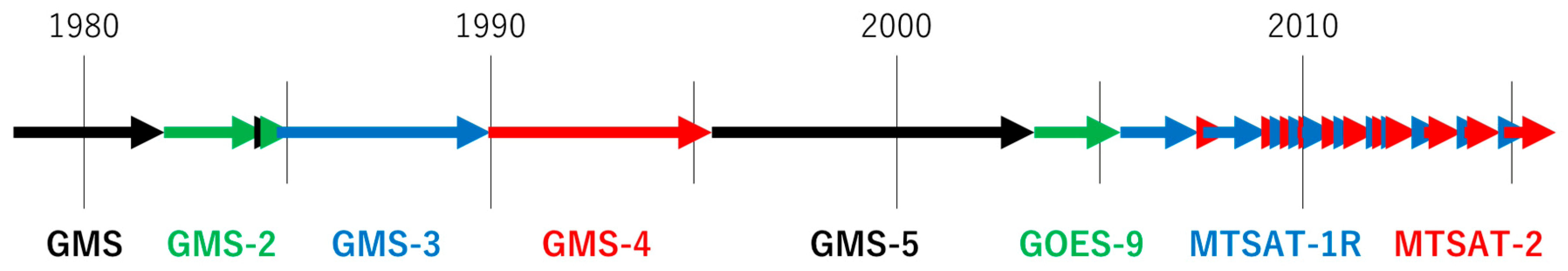
2.1. Monitored Datasets: JMA Geostationary Satellites

Since 1978, JMA has been operating nine geostationary satellites [13]. The GMS series (see Table 1) consists of five satellites: GMS, GMS-2, GMS-3, GMS-4 and GMS-5. They are spin stabilized satellites that carried the VISSR instrument and were positioned at a sub-satellite longitude of 140° E. Before 5 January 1989 (while GMS-3 was operational), they scanned the complete disk of the Earth every 3 hours [13]. Since that date, they scanned the complete disk of the Earth every hour. GMS, GMS-2, GMS-3 and GMS-4 operated one visible channel (0.50–0.70 μm) and one infrared channel (10.5–12.5 μm). GMS-5 was equipped with one visible channel (0.55–0.90 μm) and three infrared channels (6.5–7.0, 10.5–11.5 and 11.5–12.5 μm). The nadir spatial sampling resolution of VISSR data from the GMS series was 1.25 × 1.25 km for the visible channel, and 5.0 × 5.0 km for the infrared channels. The data were archived in VISSR format, which comprise level 1.0 equivalent data (non-rectified images) with calibration tables that are not fixed.
The MTSAT series (see Table 1) consists of two three-axis stabilized satellites, i.e., MTSAT-1R and MTSAT-2 [13]. MTSAT-1R carried the JAMI instrument and was positioned at sub-satellite longitudes 140° E. MTSAT-2 carried the IMAGER instrument and was positioned at sub-satellite longitudes 145° E. Those instruments scanned the complete disk of the Earth once per hour and operate one visible channel (0.55–0.90 μm) and four infrared channels (3.5–4.0, 6.5–7.0, 10.3–11.3 and 11.5–12.5 μm). The nadir spatial resolution of JAMI and IMAGER data were 1.0 × 1.0 km for the visible channel, and 4.0 × 4.0 km for the IR channels. Observed data were archived in High Rate Information Transmission (HRIT) format, which is level 1.5-equivalent data (rectified images) with fixed calibration tables. Hereinafter, the GMS and MTSAT series are referred to as JMA’s historical geostationary satellites.
On 15 November 1999, MTSAT was lost during launch due to vehicle failure. In order to secure coverage over East Asia and the Western Pacific during 2003–2005, the National Oceanic and Atmospheric Administration (NOAA) repositioned its three-axis stabilized Geostationary Operational Environmental Satellite-9 (GOES-9) satellite to sub-satellite longitudes 155° E and subsequently operated it jointly with JMA. The Imager instrument onboard NOAA GOES-9 carried one visible channel and four infrared channels [14,15], of which JMA archived the visible channel (0.55–0.75 μm) and three infrared channels (6.5–7.0, 10.2–11.2 and 11.5–12.5 μm). The nadir spatial resolution of the visible channel was 1.0 × 1.0 km, 8.0 × 8.0 km for WV channel (6.5–7.0 μm) and 4.0 × 4.0 km for the other channels. The original format of GOES-9 data is GOES Variable Format (GVAR). However, the data were archived in VISSR format with fixed calibration tables in JMA. The header part of the VISSR files comprises a minimum amount of information. Information, such as sensor temperature, was not stored. The reason why GOES-9 data were converted and stored in VISSR format was that its operation had to be taken over by JMA in a very short timeframe and VISSR format data was easy to use for JMA’s internal system and other Medium-scale Data Utilization Stations (MDUS) and Small-scale Data Utilization Stations (SDUS) users. Although GOES-9 is not JMA’s satellite, it is treated as JMA’s historical satellite during the backup period in this study.
This study only focuses on the recalibration of the IR (~11 μm) and WV (~7 μm) channels on JMA’s historical geostationary satellites. Currently, Himawari-8 is the operational satellite and Himawari-9 is the on-orbit-stand-by satellite operated by JMA. Note, that Himawari-8 and Himawari-9 are not considered in this study. Table 1 summarizes the observation period, sensor name, archived data format, channels recalibrated, manner of treating the calibration table, bit depth, and notes for each historical satellite. A graphical representation of the operational periods is presented in Figure 1.
All sensors on JMA’s historical geostationary satellites carried a blackbody for onboard calibration of WV and IR channels. Blackbody calibration reduces the effect of sensor temperature variance for the operational calibration. These onboard blackbodies were used for making the operational calibration tables.
Figure 2 shows the structure of VISSR onboard GMS-4. Five thermometers were attached on the sensor. When the sensor did not observe the Earth, a shutter appeared in front of a detector and the detector observed its radiance. This shutter functioned as a blackbody. When the detector observed the blackbody, radiance of other parts of the sensor also reached the detector. Considering those effects, the effective blackbody temperature was calculated as follows:
T E = T S + 0.120   ( T S T S M ) + 0.042   (   T S T P M ) + 0.130   (   T S T B F ) + 0.118   (   T S T B A ) 0.2 ,
where TE is the effective blackbody temperature, TS is the shutter temperature, TSM is the secondary mirror temperature, TPM is the primary mirror temperature, TBF is the baffle forward temperature and TBA is the baffle after temperature, respectively. This equation and corresponding coefficients were determined by the ground test [16].
Figure 3 shows the temperatures observed by the five thermometers on the GMS-4/VISSR instrument. During eclipse seasons (around 21 March and 21 September) diurnal variations were observed in the instrument temperatures. The observations of these five thermometers were used to calculate the effective blackbody temperature and to create the operational calibration tables for each full disk observation (slot). These tables were used to significantly reduce biases on observed temperatures caused by diurnal variations in sensor temperature.
Table 2 summarizes the operational calibration updating for GMS series satellites. Note that the data gap around 1980 is due to the lack of archived GMS data in JMA. Before March 1987, during the operations of GMS-3, the operational calibration coefficients were not updated for each slot. Some parameters (see Table 2) were calculated based on the black body and the deep space observations. The means and variances of those parameters in a day are compared with previous ones. If those were significantly different from previous ones (i.e., t-test, a 95% confidence limit), the calibration coefficients were updated based on those new parameters [9,17]. Although the effective blackbody temperature was calculated for each slot, the operational calibration tables were updated only once per day or even less frequently. Therefore, the operational IR and WV channel data probably contained a diurnally varying bias especially during eclipse seasons before March 1987. As written in Section 1, Sasaki [9] estimated the operational calibration table of the IR channel onboard GMS-2 and GMS-3 and revealed diurnal variations of the bias of 6 K at the maximum during eclipse season. Unfortunately, because the recalibration coefficients and parameters which he used are missing, we cannot remove these biases before March 1987. Furthermore, his study did not focus on GMS. As the structure of the satellite and sensor of GMS is similar to those of GMS-2 and GMS-3, the diurnal variations of the IR brightness temperature from VISSR onboard GMS is probably also similar.

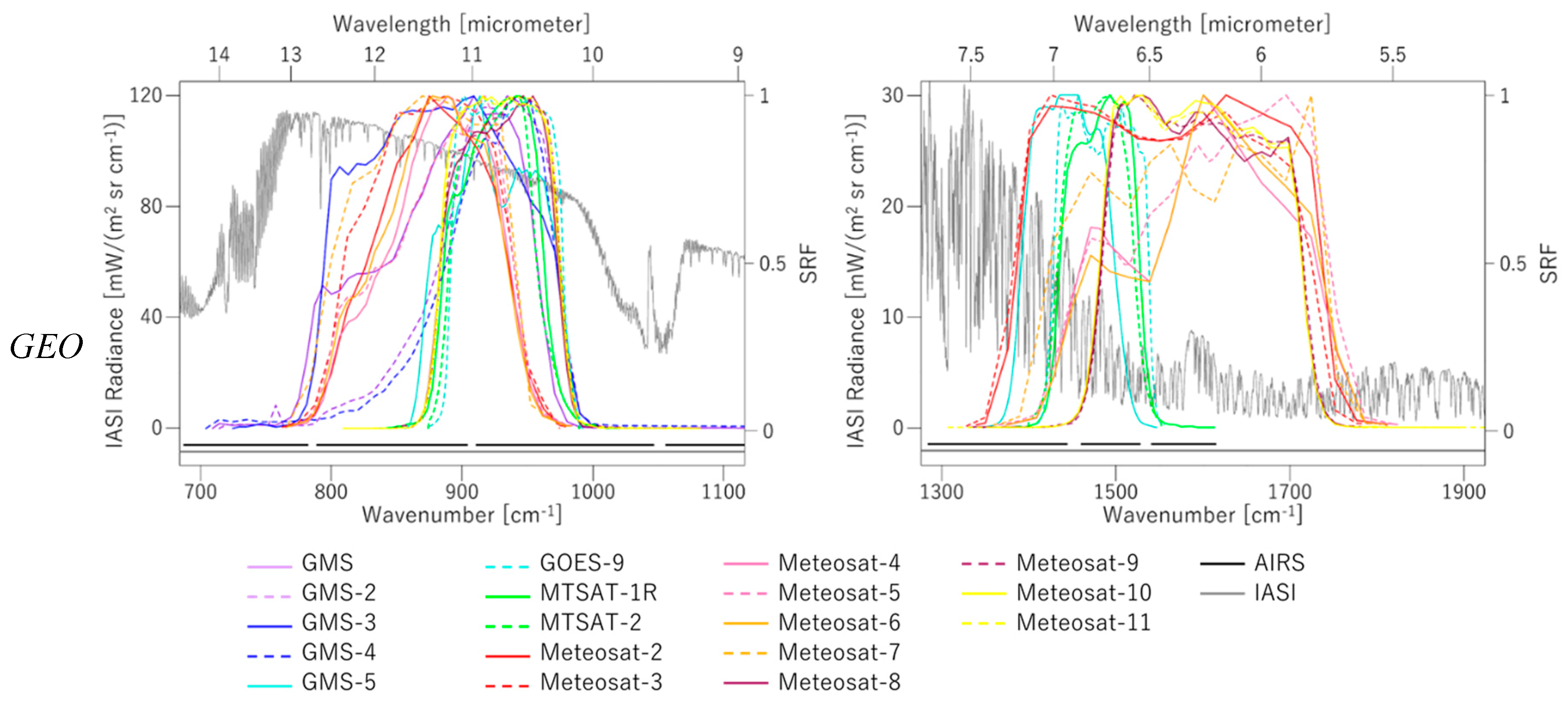
2.2. Spectral Response Functions (SRFs) of Monitored and Reference Instrument

Figure 4 illustrates the instruments’ spectral response functions (SRFs) relative to spectra as observed by AIRS and IASI. In Figure 4, the top panels show SRFs of IR and WV channels of JMA’s geostationary satellites. The corresponding channels from EUMETSAT’s geostationary satellites are shown as well for a comparison. The upper right panel suggests that the SRFs of the WV channel on JMA’s historical satellites are narrower than those on EUMETSAT’s geostationary satellites. The bottom panels in Figure 4 show the SRFs of channel 8 and 12 on HIRS that are used as reference for the recalibration of the IR and WV channel on the monitored satellites, respectively. To illustrate the difference between SRFs on HIRS/2, HIRS/3, and HIRS/4 all of SRFs are shown in the same graph. The lower right panel shows that the SRFs of HIRS/3 and 4 are narrower than those of HIRS/2 and overlap less with SRFs of the JMA’s and EUMETSAT’s geostationary satellites. John et al. [10] found that observations of HIRS/2 channel 12 correlate better with those of JMA’s and EUMETSAT’s geostationary satellites than observations of channel 12 on HIRS/3 or HIRS/4. The latter have a narrower SRF and a different central wavelength. For these reasons HIRS/2 is selected as reference instrument. The details are discussed by John et al. [10].

2.3. Reference Datasets

Table 3 lists the reference datasets used in this study. The HIRS/2 instrument is a 20-channel infrared scanning radiometer designed for atmospheric sounding. The first 12 channels operate in the longwave infrared frequencies and channels 13–19 operate in the shortwave infrared frequencies. Channel 20 is a visible channel. The instantaneous field of view (IFOV) is 20.4 km at nadir. It was operated on the TIROS-N, NOAA-6, 7, 8, 9, 10, 11, 12 and 14 satellites. The data are available from 1978 till 2006. The AIRS instrument is a sounder with 2378 spectral channels, which measures simultaneously in time and space, with an IFOV of 13.5 km at nadir. An AIRS spectrum almost covers the spectral range of the IR window channel on JMA’s geostationary satellites. However, due to several gaps in the AIRS spectrum, the spectral range of the WV channel on JMA’s geostationary satellites is only covered partly. Data are collected from 2002 till date. The IASI is an interferometer with 8461 channels with an IFOV of 12 km at nadir. It is operated on Metop-A and B satellites. The data are collected available from 2006 till date. The IASI spectrum covers the spectral range of the IR and WV channel on JMA’s geostationary satellites completely. More details on these reference instruments can be found in John et al. [10].
Instruments onboard low earth orbit satellites are adequate as reference because they have a superior calibration quality relative to that of the instruments operated onboard historical geostationary satellites [11]. The measurements from the HIRS/2 instruments onboard TIROS-N, and NOAA-6, 7, 8, 9, 10, 11, 12, 14 (1978–2006) are used as reference datasets because their operational period, which starts in 1978, overlaps with the instruments onboard GMS satellites. The hyper spectral sounder measurements from AIRS onboard Aqua (2002–date) and IASI onboard Metop-A and Metop-B (2006–date) are used because these can be convolved to make more adequate reference data, and because these can complement the time-series after the end of HIRS/2 in 2006. The combination of those reference instruments (HIRS/2, AIRS and IASI) cover the whole period of historical JMA’s satellites.

3. Methods

3.1. Principles of Common Recalibration Method

The recalibration method used in this paper was developed by John et al. [10], but briefly described here for an easy read of the paper. The method uses collocations between geostationary (GEO) and low earth orbit (LEO) observations for the recalibration of GEO IR/WV channel data. The LEO observations are used as reference data. As the IR and WV channels of historical GEO satellites have different SRFs than those of the reference instruments, Spectral Band Adjustment Factors (SBAFs) need to be applied for making data comparable. Hereto, pseudo-GEO radiances from reference instruments (HIRS/2, AIRS and IASI) were created. Linear regression coefficients, multiple linear regression coefficients, and direct convolution into GEO SRF were applied into HIRS/2, AIRS and IASI for creating pseudo-GEO radiance, respectively. The measurements for the IASI hyper spectral sounder instrument have full spectral coverage for the IR and WV channels of the target GEO satellites in this study. Therefore, the IASI radiances can be directly convolved into GEO SRFs. HIRS/2 is the broadband instruments and the measurements are not easy to be converted into the pseudo GEO radiance. The 200,000 observed IASI spectra are converted into pseudo GEO and pseudo HIRS/2 measurements. Those pairs of pseudo measurements give the coefficients for the conversion from actual HIRS/2 measurements into pseudo GEO measurements by a linear regression. The AIRS is the hyper spectral hyperspectral sounder, but does not have full spectral coverage for the IR and WV channels of the target GEO satellites in this study. Same as HIRS/2, the 200,000 IASI spectra are converted into pseudo GEO measurements and pseudo AIRS spectra. Those pairs of pseudo measurements give the coefficients for the conversion from actual AIRS spectra into pseudo GEO measurements by a multiple linear regression. Note that performing spectral band adjustment does not only mean adjustment from one broad-band sensor (e.g., GEO IR/WV channel) to another broad-band sensor, but can also mean adjustment from a hyper spectral band sensor (e.g., IASI) to a broad-band sensor.

3.2. Application of Common Recalibration Method to JMA Satellites

The adjustments needed to use the method presented by John et al. [10] for JMA satellites can be broken down into four steps. The first step is to determine and apply the SBAFs for JMA satellites. The second step is to select GEO-LEO collocations. The third step is to estimate the biases between the different reference satellites/sensors (HIRS/2, AIRS and IASI). The fourth step is to fill the bias of reference instrument by following “Prime Reference Correction.” Data from the most reliable reference instrument (Metop-A/IASI in our study) are considered as “prime reference” data. Biases between the “prime reference” and the other reference satellites/sensors (Metop-B/IASI, HIRS/2 and AIRS) need to be estimated and applied to the result of recalibration of GEO satellites. In this paper we call this correction “Prime Reference Correction.”

3.2.1. Adjusting for Spectral Band Differences

John et al. [10] used about 200,000 real IASI spectra to create SBAFs for the sensors on historical geostationary satellites relative to HIRS/2 channel 8 for the IR channel and relative to channel 12 for the WV channel. HIRS/2 channel 8 (central wavelength 11.1 µm) is a window channel, sensing the surface and the lower atmosphere, while HIRS/2 channel 12 (central wavelength 6.7 µm) is an upper tropospheric water vapor channel. Similarly, 200,000 IASI spectra were used to derive the SBAFs to convert radiances from one heritage JMA satellite to another heritage JMA satellite. The SBAFs are given in Appendix A. The SBAFs are expressed in linear function of observed radiance. The SBAF adjusted radiance ( R a d p s e u d o ) is calculated as follows:
R a d p s e u d o = o f f s e t S B A F   + s l o p e S B A F   R a d o b s ,
where the offset ( o f f s e t S B A F ) and the slope ( s l o p e S B A F ) are calculated with variances ( v a r ( o f f s e t S B A F ) ) and ( v a r ( s l o p e S B A F ) ), and a covariance ( c o v ( s l o p e S B A F , o f f s e t S B A F ) ). The uncertainties of R a d p s e u d o derived from SBAFs can be calculated by using those values.

3.2.2. GEO-LEO Collocations

SNO comparisons require the selection of observations from both instruments that represent similar viewing conditions, fields of view and observation times. In this study, we applied time check, satellite zenith angle check, environmental uniformity check and normality check to find GEO-LEO match-up that could be used for the recalibration.

Time Check

The time check defines the maximum difference in observation time between a pair of collocated pixels from LEO and GEO satellites. The thresholds used for MaxTime are listed in Table 4.
| O b s T i m e G E O O b s T i m e L E O | < M a x T i m e .

Satellite Zenith Angle Check

The satellite zenith angle (SZA) check defines the maximum difference of atmospheric path length for a collocated pixel between the LEO and GEO observation. The thresholds used for MaxZen are listed in Table 4.
| cos ( S Z A G E O ) cos ( S Z A L E O ) 1 | < M a x Z e n .

Environment Uniformity Check

In case the radiances around a collocated pixel pair have large variations (e.g., at the edge of a cloud), small image navigation errors in the GEO or LEO data can cause large differences between the observed GEO and LEO radiances. The uniformity of GEO radiance data over an EnvBox is checked with the following condition:
S t d ( E n v B o x R A D G E O ) < M a x S t d .
The thresholds used for MaxStd are listed in Table 4.
Hereto EnvLength is defined. This value represents the number of pixels for a side of EnvBox and defined in the following equation:
E n v L e n g t h = 3 × o v e r f l o o r ( N a d i r R e s o l u t i o n L E O N a d i r R e s o l u t i o n G E O ) ,
where the overfloor function derives the minimum integer which exceeds the argument. For instance, the nadir resolution of AIRS is 13.5 × 13.5 km and that of VISSR IR channel is 5 × 5 km, i.e., E n v L e g n t h = 3 × o v e r f l o o r ( 13.5 k m × 13.5 k m 5 k m × 5 k m ) = 9 . Therefore, the EnvBox of VISSR IR channel observation against AIRS is 9 × 9 pixels. The conceptual diagram of the EnvBox is shown in Figure 5.

Normality Check

In this study the observations of the used LEO instruments have a larger spatial resolution than corresponding observations of the historical GEO instruments. In order to make the LEO and GEO observations comparable, the GEO radiance data are averaged over a Field of View Box (FovBox) of the size of LEO pixels. The representativeness of the GEO radiances of the FovBox in the EnvBox is checked. The thresholds used for Gaussian values are listed in Table 4.
| M e a n ( F o v B o x R a d G E O ) M e a n ( E n v B o x R a d G E O ) | × F o v L e n g t h S t d ( E n v B o x R a d G E O ) < G a u s s i a n ,
where the FovLength (a side of FovBox) is defined as a third of EnvLength (a side of EnvBox). The conceptual diagram of the EnvBox is shown in Figure 5.

Values of Each Threshold

The checking items were taken from JMA’s GSICS study [18]. The thresholds of the above checks are listed in Table 4. The thresholds differ between the GEO satellites but also for different weather conditions. In this work we distinguish between cloudy and cloud free weather condition. If the brightness temperature of the IR channel of the GEO data at the collocated point exceeds 275 K, the scene condition is categorized as clear otherwise it is categorized as cloudy. The used thresholds are equal to the ones used within JMA’s GSICS study with considering SRF difference.
The MaxStd thresholds of the environment uniformity check slightly change between satellites, depending on SRFs. For GMS, GMS-2 and GMS-3 these thresholds are about two times higher than those of other sensors. As shown in Section 2.1, the observation frequency was small before early 1989 (mid of GMS-3). Relaxing this threshold helps to get enough colocations to calculate recalibration coefficients. Figure 6 shows the bias between the GMS/VISSR IR channel and the TIROS-N/HIRS2 channel 8. The black dots show the result when using the threshold of the IR channels from GMS-4 to MTSAT-2. The green dots show the results when using two times higher thresholds, as is done in this study. The red dots show the results when no threshold for MaxStd is used. This figure shows that doubling these thresholds helps to increase the number of collocations, and consequently the number of days for which biases (recalibration coefficients) can be estimated, and has little impact on these biases (less than 0.1 K). Using no threshold for MaxStd, on the other hand, leads to larger differences between the LEO-GEO SNOs (up to 1.0 K).

3.3. Using Operational Radiance for Linear Fit Instead of Count

The approach suggested by John et al. [10] is to calculate new calibration coefficients by linearly fitting GEO count values against LEO radiance values that have been adjusted for spectral band differences. A disadvantage of this approach is that it cannot detect diurnal or more short-term bias variations. This is because the local time of the passing reference LEO satellite is almost fixed. As written in Section 2.1, especially during the eclipse season, the operational radiance data since March 1987 contains information on variations in diurnal biases. If we used GEO count values for recalibration, the information on variations in diurnal biases, which are estimated by the blackbody calibration, could not be used. For this reason, we chose to use the operational GEO radiance data for the recalibration of JMA’s historical geostationary satellites.
Figure 7 illustrates how the correction factors are calculated. Over a period of 5 days (t – 2 days to t + 2 days), collocated data pairs (operational radiance of monitored instrument averaged over FovBox against radiance of reference instrument with SBAF applied) are linearly regressed on a day by day basis. The slope ( s l o p e c o r   ( L E O ) ) and offset ( o f f s e t c o r ( L E O ) ) of the regression line are taken as correction factors. Plots, such as the one shown in Figure 7, have uncertainties in the x-axis and y-axis. The uncertainty in the x-axis is defined as the standard deviation of operational GEO radiance over the FovBox (see Section 3.2.2). The uncertainty in the y-axis is calculated from the uncertainty of parameters of SBAFs and NEdT of each reference instruments. The linear regression line is weighted by those uncertainties of each point. The variance and covariance of the slope and offset of the regression line are also calculated considering these uncertainties. The operational calibration coefficients are consisting of slope ( s l o p e o r g ) and offset ( o f f s e t o r g ). The corrected GEO radiance ( R A D G E O ( L E O ) ) is calculated as:
R A D G E O ( L E O ) = s l o p e c o r ( L E O ) ( s l o p e o r g   D N + o f f s e t o r g ) + o f f s e t c o r ( L E O ) ,
where DN is the digital count value of the monitored instrument. Uncertainties of R A D G E O ( L E O ) can also be calculated by considering variance and covariance of s l o p e c o r ( L E O ) and o f f s e t c o r ( L E O ) . These uncertainties correspond to the uncertainties of the fit between operational GEO observations and reference instrument observations (after SBAF correction, see Equation (2)). Note that R A D G E O ( L E O ) represents the corrected GEO radiance value before prime reference correction. The prime reference correction method is explained in Section 3.4.

3.4. Route towards Applying Prime Reference Corrections

The prime reference correction method developed is described in [10]. The observations of the reference instruments are subject to differences caused by differences in their SRFs and by uncertainties in their measurements. The differences in SRFs can be corrected by performing spectral band adjustment. It is known to have systematic biases in the HIRS measurements and the aim of applying prime reference corrections is to remove the systematic biases between different reference instruments (LEO satellites) by anchoring the observations of these instruments to a pre-defined prime reference. In our study IASI on Metop-A is taken as the prime reference. The observations of the other reference instruments are adjusted to this prime reference by using the monitored satellites (GEO satellites) as a “bridge.” It is assumed that the biases between the reference instruments remain constant in time. In order to correct for SRF differences, the measurements of the two reference instruments are adjusted to the SRF of the geostationary satellite. The double difference is derived from collocated pairs of monitored and reference satellite pixel radiances collected during overlapping periods of the two reference satellites, i.e., radiance pairs of (i) R A D G E O   &   R A D L E O 1 and (ii) R A D G E O   &   R A D L E O 2 . After adjusting the radiances of both reference satellites to the spectral response of the monitored satellites, the correction coefficients can be determined using linear regression (see Figure 7). Subsequently, the corrected radiance of the monitored instrument can be computed relative to the reference satellite 1 ( R A D G E O ( L E O 1 ) ) and relative to the reference satellite 2 ( R A D G E O ( L E O 2 ) ) as follows:
R A D G E O ( L E O 1 ) = s l o p e c o r ( L E O 1 ) ( R A D G E O ) + o f f s e t c o r ( L E O 1 ) ,
R A D G E O ( L E O 2 ) = s l o p e c o r ( L E O 2 ) ( R A D G E O ) + o f f s e t c o r ( L E O 2 ) .
If measurements of both reference satellites would be perfectly unbiased, R A D G E O ( L E O 1 ) and R A D G E O ( L E O 2 ) would be equal. However, as explained above, systematic biases exist between the reference instruments. The “prime” corrections relate the radiances of the “prime” reference satellite to the radiances of another reference satellite as follows:
R A D G E O ( L E O 2 ) = s l o p e p r i m e   R A D G E O ( L E O 1 ) + o f f s e t p r i m e .
The correction slopes and offsets of Equations (9) and (10) can be used to derive the “prime” correction slope ( s l o p e p r i m e ) and offset ( o f f s e t p r i m e ) using:
s l o p e p r i m e   = s l o p e c o r ( L E O 2 ) s l o p e c o r ( L E O 1 ) ,
o f f s e t p r i m e = o f f s e t c o r ( L E O 2 ) s l o p e c o r ( L E O 2 ) s l o p e c o r ( L E O 1 ) o f f s e t c o r ( L E O 1 ) .
In this paper the “prime” corrections are derived in two steps. Firstly, the “prime” slope and the “prime” offset, including variance and covariance, are calculated on a day-by-day basis during the overlapping period of two reference satellites. Secondly, the day-by-day slopes and offsets are averaged over the overlapping period. Those day-by-day slopes and offsets are also used to calculate the variance and covariance of the averaged slope and offset.
Once the corrections between the “prime” reference instrument (Metop-A/IASI) and the second reference instrument (AIRS) are determined, the “prime” corrections can be propagated further to the earlier reference satellites. Hereto, these corrections are used to adjust the second reference instrument to the “prime” reference, referred to as pseudo “prime” reference. The “prime” corrections for the third reference instrument can be derived from pairs of pseudo “prime” reference (i.e., second reference) and monitored instrument radiances, and pairs of third reference and monitored instrument radiances collected for their overlapping period, i.e., apply Equations (9)–(13). This process is repeated till “prime” corrections have been derived for the entire series of reference instruments. The variances and covariances are propagated back in time. As a result, variances and covariances will be largest for the early reference instruments.

4. Results

4.1. Standard Radiance

In order to determine the biases of operational GEO radiance, we follow the GSICS approach, which needs information of a reference radiance, i.e., the standard radiance. The standard radiance is defined as the radiance value observed by the satellite instrument for one reference target. The value of the standard radiance depends on the instrument’s SRF, and thus differs from instrument to instrument. The standard radiances of the historical JMA satellites were calculated for each channel using RTTOV-11 with the 1976 US Standard Atmosphere for nadir condition in clear sky at night over an ocean surface with a Sea Surface Temperature (SST) of 288.15 K and a wind speed of 7 m/s. These values are similar to those used in JMA’s GSICS framework for Himawari-8 [18]. Table 5 lists the standard radiance values and associated brightness temperatures for each JMA historical satellite. The differences of those values are caused by differences in their SRFs. The conversion between radiance and brightness temperature uses Sensor Planck Function, which is calculated by Tahara [19] (see Appendix B).

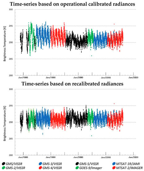
4.2. Evaluation of Time-Series of Recalibrated Data before Prime Reference Correction

The calibration tables of the IR and WV channels onboard historical JMA’s geostationary satellites are re-created using the common recalibration method adopted for all JMA satellites. In this paper, the radiance based on the operational calibration table is referred to as the operational radiance, and the radiance based on this re-created calibration table is referred to as the corrected radiance. For easy understanding, biases are shown in brightness temperature.
As a first step, we evaluated the bias of operational radiance against each LEO reference radiance observation. The SBAFs are applied to convert the radiances of the LEO reference instrument to radiances of the GEO monitored instrument, but no prime reference correction was applied. Figure 8 shows the biases of the operational radiance of IR and WV channels onboard JMA’s historical satellites against the LEO radiances at standard radiance. Note that each data point in those figures has uncertainty bars (1σ), which are calculated from uncertainty of the linear regression of LEO radiance and GEO operational radiances as discussed in Section 3.3. However, those values are very small. The average of uncertainty for GMS-5/VISSR WV channel against NOAA11/HIRS/2 ch12 is 0.01 K. Others are smaller than this. The figures reveal that the biases with the reference instruments are generally smaller than 2 K for the IR and WV channels. During the era of GMS/GMS-2/GMS-3/GMS-4 the biases tend to show strong seasonal cycles. During the GMS-5/GOES-9/MTSAT-1R/MTSAT-2 era these seasonal variations are an order of magnitude smaller. In addition, these figures show that there are steady differences between biases estimated by HIRS/2 and those by Aqua/AIRS. A typical example is the biases of the GOES-9 WV channel (deep green lines and light green lines in the bottom panel). However, those steady differences would be eliminated by the prime reference correction. The large variation in the biases of GMS-5/VISSR WV channel against NOAA-14/HIRS/2 ch12 is caused by the difference between their SRFs. Note that the data gap around 1980 is due to the lack of archived GMS data.

4.3. Evaluation of Time-Series of Recalibrated Data after Prime Reference Correction

As a second step, the prime reference correction is applied to remove the bias of the LEO satellite instruments against the prime reference (Metop-A/IASI). The parameter of the prime reference correction is introduced by the double difference method discussed in Section 3.4. The prime reference correction parameters are shown in Appendix C. If several LEO satellites are collocated with a GEO satellite at one day, the several pairs of recalibration coefficients based on each reference sensors after the prime reference correction are merged into one pair of the coefficients based on the uncertainties of those coefficients.
Figure 9 shows the difference between the operational and corrected radiances after applying the prime reference correction. Similar to Figure 8, each bias in these panels is provided with an uncertainty bar (1σ). For the IR channel, Figure 9 (upper panel) reveals significant seasonal changes in radiometric biases for the operational radiances of GMS to GMS-4. The amplitudes of the biases are 2 K for GMS, 3 K for GMS-2, 2 K for GMS-3 and 1 K for GMS-4. All satellites have a positive bias in winter time and a negative bias in summer time. It is suggested that these biases are related to variations in the sensor temperature. As shown in Section 2.1, the effective blackbody temperature of the VISSR instrument is calculated from the shutter (blackbody) temperature and from the temperatures of other parts of the instrument. The north-south asymmetry of the satellites shape attributes to gradients in temperature at each part of the VISSR instrument caused by seasonal changes in the position of the sun relative to the satellite or diurnal changes in the satellite illumination. These changes lead to seasonal or diurnal variations in the calibration bias. On GMS-4 the number of thermometers, the positions of the thermometers, and the equation for calculating the effective blackbody temperature were improved as compared to GMS/GMS-2/GMS-3 [16]. Although these improvements reduced the amplitude of radiometric bias of GMS-4 from about 2 K to about 1 K, the overall magnitude of the biases remained similar, with about –0.5 K for GMS, 0.0 K for GMS-2, 0.7 K for GMS-3 and 0.5 K for GMS-4.
For GMS-5, the number of thermometers, the positions of the thermometers, and the equation for the effective the blackbody temperature were further improved [20]. Moreover, the structure of observing blackbody changed. Before GMS-4, a shutter appearing in front of the detector behaved as a blackbody. Instead of using a blackbody shutter, GMS-5 and the later satellites used mirrors that appeared in front of the detector. These mirrors reflect the radiation emitted by the blackbody, which is attached inside the instrument on those satellites and the radiation reaches the detecting elements of those instruments [21]. These improvements resulted in a significant reduction of the amplitude of biases for the operational radiances. The operational IR radiances of GMS-5 and GOES-9 reveal half yearly variations in radiometric biases, with amplitudes of about 0.2 and 0.1 K, respectively. These variations may also be related to variations in sensor temperature during the eclipse season. The radiometric bias of GMS-5 has a magnitude of about −0.7 K. A small jump of the radiometric bias is found in GOES-9 in December 2003, with a radiometric bias of −0.2 K before the jump and 0.0 K after the jump. For MTSAT-1R and MTSAT-2, small seasonal cycles in radiometric biases are found, with amplitudes smaller than 0.1 K for both satellites. However, before 2007, the amplitudes of the radiometric biases on MTSAT-1R were larger, about 0.4 K. The radiometric biases of MTSAT-1R and MTSAT-2 are −0.3 and 0.1 K, respectively.
For the WV channel, Figure 9 (bottom panel) did not reveal significant seasonal changes in radiometric biases for GOES-9/MTSAT-1R/MTSAT-2. For GMS-5, the amplitude of the seasonal variation in biases is about 0.5 K. The radiometric biases of GMS-5, MTSAT-1R and MTSAT-2 have a magnitude of about −0.3, 0.3 and −0.2 K, respectively. Similar to the IR channel, a large jump in the radiometric bias of GOES-9 is observed in December 2003, with a radiometric bias of −0.1 K before the jump and 0.6 K after the jump. Till August 2002, the GMS-5 biases show large variations because HIRS/2 is the only reference instrument. The SRFs of the WV channel onboard historical JMA satellites, such as GMS-5, differ considerably from those of HIRS/2 ch12 (see Figure 4). This mismatch explains part of the uncertainty in the recalibrated radiances. On the other hand, from August 2002 onwards, Aqua/AIRS was also used as reference instrument. The conclusive recalibration coefficients are weighted averages of recalibration coefficients derived from each reference instrument. The weights depend on the uncertainties of recalibration coefficients derived from each reference instrument. As the uncertainties of recalibration coefficients derived from AIRS are much smaller than those from HIRS/2, the conclusive recalibration coefficients are almost the same as those derived from AIRS alone and the uncertainties are also small from August 2002 onwards.
Figure 10 shows the average of uncertainty bars (1σ) of each GEO instrument shown in Figure 9. The large uncertainties for the old GEO instruments are due to multiple uncertainties of SBAFs from one GEO instrument to another GEO instrument and uncertainties of double difference for estimating the bias of one LEO instrument against another LEO instrument.

4.4. Applying Recalibration Coefficients to Actual Data

Recalibrated coefficients are applied to actual observation data. Herein, two terms, sensor equivalent radiance and baseline sensor normalized radiance, are defined. Sensor equivalent radiance is the radiance based on the SRFs of each observing sensor. As discussed in Section 4.1, the difference between instrument SRFs explains the differences in radiances that are observed for same target. This is why it is difficult to spot temporal trends over target areas by just analyzing time-series of observations from different instruments. Baseline sensor normalized radiances are radiances that are adjusted to the SRF of a common sensor (the baseline sensor) by SBAFs. The SRF of MTSAT-2/IMAGER is selected as the common baseline sensor for the normalized radiance in this paper.
Figure 11 and Figure 12 show, for JMA’s geostationary satellites, time-series of daily average clear sky radiances for sub-satellite area (−30° < latitude < 30°, sub_satellite_longitude −30° < longitude < sub_satellite_longitude +30°) in brightness temperature units (K) for the IR and WV channel, respectively. These figures present the operational (Figure 11) and recalibrated (Figure 12) time-series. The data points represent daily brightness temperatures that are derived from 6 hourly radiance averages. If the brightness temperature of a pixel of the IR channel exceeds 275 K, the target pixel is considered clear. The shaded areas in the lower panel represent the 1 sigma uncertainty due to the recalibration.
For the IR channel, the top and bottom graph represents the operational (not-recalibrated) and recalibrated brightness temperature in baseline sensor normalized radiance, respectively. The comparison between those graphs shows the impact of the recalibration with using LEO (reference) instruments. In the top graph, there are bigger seasonal variations of observed brightness temperature till GMS-4 as compared to later satellites. Furthermore, for GMS-5 the operational brightness temperature is relatively low. However, the annual variability of the recalibrated brightness temperature till GMS-4 are almost the same as for GMS-5 or later. The temporal average of the observed brightness temperature for GMS-5 is almost the same as for the other instruments. The large uncertainties for the old GEO instruments are due to different sources of uncertainties in the SBAFs and the double difference approach.
A similar impact can be discussed for the WV channel. The comparison of both graphs in Figure 12 shows that the temporal averages of observed brightness temperature from each instrument became more equal by recalibration. The observed brightness temperature by of GMS-5 is slightly lower than that of GOES-9 in the top graph, but almost the same in the bottom graph.
Table 6 summarizes the statistics for the baseline sensor normalized brightness temperatures based on the radiances. This table suggests that the recalibration helped to reduce the temporal noise of the GEO observation and to reduce the bias between different GEO instrument observations.

5. Discussion

5.1. SRF of GMS5/VISSR WV Channel

Bréon et al. [22] pointed out that the operational SRF of the GMS-5/VISSR WV channel provided by the satellite sensor vendor had been contaminated by atmospheric absorption, and suggested corrected SRF (shown in Figure 13). They collect the information about the condition (the air temperature, the humidity and the distance between the light sources and the instrument) for the ground testing of the instrument’s SRF. An atmospheric transmission model with this information and the operational SRF enabled to create the expected SRF without the contamination by atmospheric absorption.
Kobayashi et al. [23] used RTTOV-10 to evaluate the corrected SRFs, and found that the erroneous SRF causes a bias of about 0.6 K in brightness temperature at typical atmospheric conditions in mid-latitudes. In this study we applied another approach to evaluate the correctness of the corrected SRF, using pseudo GMS-5/VISSR brightness temperatures based on Aqua/AIRS observations. The method to produce pseudo GMS-5/VISSR WV radiances from Aqua/AIRS was developed by John et al. [10]. Pseudo GMS-5/VISSR brightness temperatures were calculated for all collocations between Aqua/AIRS and GMS-5/VISSR during the period August 2002 till May 2003 (all overlap period between GMS-5 and Aqua). Figure 14 shows the difference between observed GMS-5/VISSR brightness temperatures and pseudo GMS-5/VISSR brightness temperatures converted from Aqua/AIRS observations for all collocations. The left panel of Figure 14 shows the relationship between pseudo GMS-5 WV radiances calculated with the operational SRF and GMS-5 observed radiances. The right panel of Figure 14 shows the relationship between pseudo GMS-5 WV radiances calculated with the corrected SRF suggested by Bréon et al., and GMS-5 observed radiances. This result suggests that the corrected SRF is more consistent with AIRS (more reliable) observations than the operational SRF. The average of biases on the left panel and the right panel of Figure 14 are 1.03 and 0.25 K, respectively. The difference between them is about 0.78 K, which is consistent with the evaluation by Kobayashi et al. [23]. This result made us decide to use, instead of operational SRF, the corrected SRF suggested by Bréon et al., for recalibration of GMS-5/VISSR WV channel presented in this study.

5.2. Variations in Diurnal Biases

The GOES-9, MTSAT-1R and MTSAT-2 satellites are three-axis stabilized satellites (see Section 2.1). The sensors onboard these types of satellites are subject to diurnal variations in temperature, which results in diurnal variations in the measurement biases. Figure 15 shows the measurement biases of MTSAT-1R/JAMI at each time of days for both of the IR and WV channels. This figure shows that the measurement biases correlate with the observation times. The measurement biases are calculated relative to the measurements of two reference satellites, using collocations collected during the month December 2009. This month is outside the eclipse season. It is expected that the diurnal biases get bigger during the eclipse season.
Similar to Figure 15, the left panel of Figure 16 shows the measurement biases for the IR channel of GMS-4/VISSR calculated from collocations with HIRS/2 during December 1992. Although the GMS-4 is a spin stabilized satellite, it also shows diurnal variations in the measurement biases. The right panel of Figure 16 shows, for the five thermometers that are used to calculate the effective blackbody temperature, the differences between period averaged thermometer temperature and instantaneous thermometer temperature. This panel confirms that the measurements of IR channel of GSM-4/VISSR are subject to diurnal variations due to diurnal variations in the temperatures of the five thermometers. In this study, such diurnal biases are not considered for the prime reference correction. Further studies are necessary for the removal of those diurnal biases and for taking account of them for the prime reference correction.

6. Conclusions

A common recalibration approach was applied to the IR and WV channels of the VISSR, JAMI, and IMAGER instruments from the JMA’s historical geostationary satellites. Data from the IASI, AIRS and HIRS/2 instruments were used as reference for recalibration. The recalibrated IR data from the old JMA satellites (GMS to GMS-4) reveal significant seasonal changes in radiometric biases during their 17 years of operation (1978-1995). This suggests that the sensors on the old JMA satellites were strongly affected by seasonal variations in solar illumination. The amplitude of the biases differs from satellite to satellite, and tends to be smaller for more recent satellites (from 3 to 1 K). From GMS-5 till MTSAT-2 the biases are smaller than 0.7 K and the seasonal variations have a relatively small amplitude, i.e., smaller than 0.4 K. Apart from GMS-5, the time-series of recalibrated WV channel radiances does not reveal seasonal variations. The seasonal variations in the WV channel of GMS-5 have an amplitude of about 0.5 K. The biases for GMS-5, MTSAT-1R and MTSAT-2 are smaller than 0.3 K. In December 2003, a large jump was observed in the radiometric bias of the IR and WV channel on GOES-9, with the bias jumping from −0.2 to 0.0 K for the IR channel and from −0.1 to 0.6 K for the WV channel. This jump was caused by the update of ground processing modules.
The comparison of the operational calibrated and recalibrated time-series of the baseline sensor normalized radiances confirms that the recalibration based on the method from John et al. [10] resulted in a time-series with significantly smaller sensor-to-sensor jumps and comparable annual variations for each sensor. This conclusion applies to both the IR and WV channel time-series.
Note that the method in this study cannot correct for variations in diurnal biases, which are especially problematic for data that were archived before March 1987. The operational calibration coefficients of those data were updated once a day or less. Since March 1987, the sensor temperature was used to update the operational calibration table for every slot. As a result, the radiometric biases of those operational data showed less diurnal variations.
This study also confirms the validity of the corrected SRF of the GMS-5/VISSR WV channel as suggested by Bréon et al. [22]. The operational SRF contains an error due to atmospheric absorption contamination.
This research contributes to the WMO initiative Sustained and Coordinated Processing of Environmental Satellite data for Climate Monitoring (SCOPE-CM) project No. 6: Inter-calibration of imager observations from time-series of geostationary satellites (IOGEO), which aims at establishing spatially and temporally homogeneous radiance data of all geostationary satellites. The Fundamental Climate Data Records (FCDR) presented in this paper is a contribution to the SCOPE-CM IOGEO project. In this project, the recalibration of the visible channel is also a target, developing and applying a common method to the visible channel onboard JMA’s and EUMETSAT’s historical satellites is future work.

Author Contributions

Conceptualization, all authors.; data curation, T.T. and V.O.J.; formal analysis, T.T., V.O.J. and R.A.R.; investigation, T.T. and V.O.J.; methodology, all authors; project administration, J.S. and R.A.R.; software, V.O.J. and T.T.; supervision, V.O.J., R.A.R., T.H. and J.S.; validation, T.T. and V.O.J.; visualization, T.T.; writing—original draft preparation, T.T. and R.A.R., writing—review & editing, all authors.

Funding

This research was carried out under collaboration between JMA and EUMETSAT through a visiting scientist activity at EUMETSAT and was funded by a Fellowship Program by the Ministry of Education, Culture, Sports, Science and Technology of the Japanese Government.

Acknowledgments

The authors would like to thank P. Brunel for creating the coefficients for calculating the standard radiance of sensors on JMA’s historical satellites with RTTOV based on JMA’s request. The authors also would like to thank University of Wisconsin for archiving GMS/VISSR data and providing them to JMA. The authors also would like to show their appreciation to JMA’s technical staffs, M. Takahashi and A. Okuyama for advising related to GSICS techniques, K. Date for giving the information about historical JMA’s satellite format and their onboard processes, and S. Kobayashi advancing from the side of climate dataset user. We are also grateful to the referees for useful comments.

Conflicts of Interest

The authors declare no conflict of interest.

Abbreviations

The following abbreviations are used in this manuscript:
AIRSAtmospheric Infrared Sounder
CDRClimate Data Records
DDDouble Difference
EUMETSATEuropean Organization for the Exploitation of Meteorological Satellites
FCDRFundamental Climate Data Records
FoVField of View
GEOGeostationary
GMSGeostationary Metrological Satellite
GOESGeostationary Operational Environmental Satellite
GSICSGlobal Space-based Inter-calibration System
GVARGOES Variable Format
HIRSHigh-Resolution Infrared Radiation Sounder
HRITHigh Rate Information Transmission
IASIInfrared Atmospheric Sounding Interferometer
IFOVInstantaneous field of view
IOGEOInter-calibration of imager observations from time-series of geostationary satellites
IRInfrared
JAMIJapanese Advanced Meteorological Imager
JMAJapan Meteorological Agency
JRA-25Japanese 25-year Reanalysis
LEOLow earth orbit
MDUSMedium-scale Data Utilization Stations
MTSATMulti-functional Transport Satellite
NOAANational Oceanic and Atmospheric Administration
SBAFSpectral Band Adjustment Factor
SCOPE-CMSustained and Coordinated Processing of Environmental Satellite data for Climate Monitoring
SDUSSmall-scale Data Utilization Stations
SNOSimultaneous Nadir Overpass
SRFSpectral Response Function
SSTSea Surface Temperature
SZASatellite zenith angle
VISSRVisible and Infrared Spin Scan Radiometer
WMOWorld Meteorological Organization
WVWater Vapor

Appendix A. Spectral Adjustment Factors (SBAFs) for Historical JMA’s Satellites and HIRS2

The Spectral Adjustment Factors (SBAFs) are used to convert radiances from one instrument to another instrument.
The SBAFs are applied as in the following equation
R a d p s e u d o = o f f s e t S B A F   + s l o p e S B A F   R a d o b s .
The uncertainties of SBAFs are given by the following equation
v a r ( R A D p s e u d o ) = v a r ( o f f s e t S B A F ) + v a r ( s l o p e S B A F )   R A D o b s 2 + 2   c o v ( o f f s e t S B A F , s l o p e S B A F )   R A D o b s .
The parameters for each instrument are listed in the following tables
Table A1. SBAFs for the IR channel radiances from channel 8 on HIRS2 to those of the IR channel on the historical JMA’s satellites (unit: mW/(m2 sr cm−1)).
Sensor to
GMS/VISSRGMS-2/VISSRGMS-3/VISSRGMS-4/VISSRGMS-5/VISSRGOES-9/ImagerMTSAT-1R/JAMIMTSAT-2/IMAGER
Sensor fromTIROS-N/HIRS2offsetSBAF1.91388 × 1001.76601 × 10−12.01927 × 1003.41112 × 10−1−4.77384 × 10⁻¹−7.68048 × 10⁻¹−6.33724 × 10⁻¹−6.92769 × 10⁻¹
slopeSBAF9.90390 × 10−19.66809 × 10−19.93578 × 10−19.55282 × 10−19.67450 × 10−19.57915 × 10−19.67629 × 10−19.68974 × 10⁻¹
var(offsetSBAF)1.69848 × 10−42.66605 × 10−42.39072 × 10−43.55870 × 10−44.51932 × 10−48.54050 × 10−45.15838 × 10−45.37767 × 10−4
var(slopeSBAF)1.78400 × 10−82.80028 × 10−82.51108 × 10−83.73787 × 10−84.74685 × 10−88.97049 × 10−85.41809 × 10−85.64841 × 10−8
cov(offsetSBAF,slopeSBAF)−1.68816 × 10⁻⁶−2.64985 × 10⁻⁶−2.37619 × 10⁻⁶−3.53707 × 10⁻⁶−4.49185 × 10⁻⁶−8.48861 × 10⁻⁶−5.12704 × 10⁻⁶−5.34499 × 10⁻⁶
NOAA06/HIRS2offsetSBAF2.02750 × 1002.82410 × 10−12.13380 × 1004.45310 × 10−1−3.72665 × 10⁻¹−6.65897 × 10⁻¹−5.29343 × 10⁻¹−5.88399 × 10⁻¹
slopeSBAF9.87999 × 10−19.64529 × 10−19.91174 × 10−19.53033 × 10−19.65181 × 10−19.55685 × 10−19.65363 × 10−19.66707 × 10⁻¹
var(offsetSBAF)2.29125 × 10−42.21170 × 10−43.10005 × 10−43.04405 × 10−43.82866 × 10−47.55096 × 10−44.39502 × 10−44.58042 × 10−4
var(slopeSBAF)2.40049 × 10−82.31714 × 10−83.24785 × 10−83.18917 × 10−84.01118 × 10−87.91094 × 10−84.60455 × 10−84.79879 × 10−8
cov(offsetSBAF,slopeSBAF)−2.27427 × 10⁻⁶−2.19531 × 10⁻⁶−3.07708 × 10⁻⁶−3.02149 × 10⁻⁶−3.80028 × 10⁻⁶−7.49500 × 10⁻⁶−4.36245 × 10⁻⁶−4.54647 × 10⁻⁶
NOAA07/HIRS2offsetSBAF1.87218 × 1001.39050 × 10−11.97705 × 1003.04381 × 10−1−5.14368 × 10⁻¹−8.03609 × 10⁻¹−6.70530 × 10⁻¹−7.29586 × 10⁻¹
slopeSBAF9.86798 × 10−19.63269 × 10−19.89978 × 10−19.51780 × 10−19.63902 × 10−19.54391 × 10−19.64078 × 10−19.65417 × 10⁻¹
var(offsetSBAF)1.52417 × 10−43.13191 × 10−42.13905 × 10−44.08756 × 10−45.10545 × 10−49.32785 × 10−45.78235 × 10−46.01147 × 10−4
var(slopeSBAF)1.58798 × 10−83.26304 × 10−82.22860 × 10−84.25870 × 10−85.31920 × 10−89.71839 × 10−86.02444 × 10−86.26316 × 10−8
cov(offsetSBAF,slopeSBAF)−1.50882 × 10⁻⁶−3.10037 × 10⁻⁶−2.11750 × 10⁻⁶−4.04640 × 10⁻⁶−5.05403 × 10⁻⁶−9.23391 × 10⁻⁶−5.72412 × 10⁻⁶−5.95093 × 10⁻⁶
NOAA08/HIRS2offsetSBAF1.97461 × 1002.33758 × 10−12.08041 × 1003.97508 × 10−1−4.20725 × 10⁻¹−7.12543 × 10⁻¹−5.77219 × 10⁻¹−6.36274 × 10⁻¹
slopeSBAF9.87304 × 10−19.63819 × 10−19.90480 × 10−19.52329 × 10−19.64464 × 10−19.54965 × 10−19.64644 × 10−19.65986 × 10⁻¹
var(offsetSBAF)1.99938 × 10−42.52768 × 10−42.73774 × 10−43.40659 × 10−44.27128 × 10−48.17494 × 10−44.87692 × 10−45.07741 × 10−4
var(slopeSBAF)2.08953 × 10−82.64165 × 10−82.86118 × 10−83.56019 × 10−84.46386 × 10−88.54353 × 10−85.09680 × 10−85.30634 × 10−8
cov(offsetSBAF,slopeSBAF)−1.98218 × 10⁻⁶−2.50593 × 10⁻⁶−2.71419 × 10⁻⁶−3.37728 × 10⁻⁶−4.23452 × 10⁻⁶−8.10459 × 10⁻⁶−4.83495 × 10⁻⁶−5.03372 × 10⁻⁶
NOAA09/HIRS2offsetSBAF1.91769 × 1001.81067 × 10−12.02298 × 1003.45683 × 10−1−4.72833 × 10⁻¹−7.63243 × 10⁻¹−6.29145 × 10⁻¹−6.88200 × 10⁻¹
slopeSBAF9.87255 × 10−19.63741 × 10−19.90435 × 10−19.52249 × 10−19.64379 × 10−19.54872 × 10−19.64557 × 10−19.65898 × 10⁻¹
var(offsetSBAF)1.72326 × 10−42.83934 × 10−42.39477 × 10−43.75907 × 10−44.70900 × 10−48.78543 × 10−45.35377 × 10−45.57029 × 10−4
var(slopeSBAF)1.79872 × 10−82.96367 × 10−82.49963 × 10−83.92367 × 10−84.91520 × 10−89.17013 × 10−85.58820 × 10−85.81420 × 10−8
cov(offsetSBAF,slopeSBAF)−1.70743 × 10⁻⁶−2.81325 × 10⁻⁶−2.37277 × 10⁻⁶−3.72453 × 10⁻⁶−4.66574 × 10⁻⁶−8.70472 × 10⁻⁶−5.30459 × 10⁻⁶−5.51911 × 10⁻⁶
NOAA10/HIRS2offsetSBAF1.94652 × 1002.07778 × 10−12.05207 × 1003.71955 × 10−1−4.46412 × 10⁻¹−7.37530 × 10⁻¹−6.02814 × 10⁻¹−6.61868 × 10⁻¹
slopeSBAF9.87366 × 10−19.63865 × 10−19.90544 × 10−19.52372 × 10−19.64506 × 10−19.55002 × 10−19.64685 × 10−19.66026 × 10⁻¹
var(offsetSBAF)1.85616 × 10−42.67878 × 10−42.56116 × 10−43.57780 × 10−44.48570 × 10−48.47561 × 10−45.11096 × 10−45.31964 × 10−4
var(slopeSBAF)1.93900 × 10−82.79833 × 10−82.67546 × 10−83.73747 × 10−84.68588 × 10−88.85386 × 10−85.33905 × 10−85.55705 × 10−8
cov(offsetSBAF,slopeSBAF)−1.83982 × 10⁻⁶−2.65519 × 10⁻⁶−2.53861 × 10⁻⁶−3.54629 × 10⁻⁶−4.44619 × 10⁻⁶−8.40097 × 10⁻⁶−5.06596 × 10⁻⁶−5.27280 × 10⁻⁶
NOAA11/HIRS2offsetSBAF2.03568 × 1002.89736 × 10−12.14209 × 1004.52470 × 10−1−3.65458 × 10⁻¹−6.58983 × 10⁻¹−5.22169 × 10⁻¹−5.81224 × 10⁻¹
slopeSBAF9.88776 × 10−19.65294 × 10−19.91952 × 10−19.53790 × 10−19.65948 × 10−19.56447 × 10−19.66131 × 10−19.67475 × 10⁻¹
var(offsetSBAF)2.33900 × 10−42.12582 × 10−43.16437 × 10−42.94454 × 10−43.71777 × 10−47.39774 × 10−44.27684 × 10−44.46036 × 10−4
var(slopeSBAF)2.45477 × 10−82.23104 × 10−83.32099 × 10−83.09028 × 10−83.90178 × 10−87.76388 × 10−84.48852 × 10−84.68112 × 10−8
cov(offsetSBAF,slopeSBAF)−2.32367 × 10⁻⁶−2.11189 × 10⁻⁶−3.14363 × 10⁻⁶−2.92524 × 10⁻⁶−3.69340 × 10⁻⁶−7.34925 × 10⁻⁶−4.24881 × 10⁻⁶−4.43112 × 10⁻⁶
NOAA12/HIRS2offsetSBAF1.95577 × 1002.16297 × 10−12.06140 × 1003.80329 × 10−1−4.37996 × 10⁻¹−7.29355 × 10⁻¹−5.94429 × 10⁻¹−6.53484 × 10⁻¹
slopeSBAF9.87367 × 10−19.63871 × 10−19.90545 × 10−19.52379 × 10−19.64514 × 10−19.55011 × 10−19.64693 × 10−19.66034 × 10⁻¹
var(offsetSBAF)1.90436 × 10−42.62360 × 10−42.62127 × 10−43.51532 × 10−44.40846 × 10−48.36786 × 10−45.02700 × 10−45.23283 × 10−4
var(slopeSBAF)1.98972 × 10−82.74120 × 10−82.73877 × 10−83.67290 × 10−84.60607 × 10−88.74295 × 10−85.25234 × 10−85.46739 × 10−8
cov(offsetSBAF,slopeSBAF)−1.88776 × 10⁻⁶−2.60072 × 10⁻⁶−2.59842 × 10⁻⁶−3.48467 × 10⁻⁶−4.37003 × 10⁻⁶−8.29491 × 10⁻⁶−4.98318 × 10⁻⁶−5.18721 × 10⁻⁶
NOAA14/HIRS2offsetSBAF1.94430 × 1002.05639 × 10−12.04984 × 1003.69835 × 10−1−4.48538 × 10⁻¹−7.39631 × 10⁻¹−6.04935 × 10⁻¹−6.63989 × 10⁻¹
slopeSBAF9.87541 × 10−19.64035 × 10−19.90719 × 10−19.52540 × 10−19.64676 × 10−19.55170 × 10−19.64855 × 10−19.66197 × 10⁻¹
var(offsetSBAF)1.84538 × 10−42.67504 × 10−42.55042 × 10−43.57283 × 10−44.48473 × 10−48.47573 × 10−45.11111 × 10−45.32036 × 10−4
var(slopeSBAF)1.92833 × 10−82.79528 × 10−82.66507 × 10−83.73343 × 10−84.68632 × 10−88.85673 × 10−85.34086 × 10−85.55951 × 10−8
cov(offsetSBAF,slopeSBAF)−1.82941 × 10⁻⁶−2.65189 × 10⁻⁶−2.52836 × 10⁻⁶−3.54192 × 10⁻⁶−4.44593 × 10⁻⁶−8.40241 × 10⁻⁶−5.06689 × 10⁻⁶−5.27433 × 10⁻⁶
Table A2. SBAFs for the WV channel radiances from channel 12 on HIRS2 to those of the WV channel on the historical JMA’s satellites (unit: mW/(m2 sr cm−1)).
Sensor to
GMS-5/VISSRGOES-9/ImagerMTSAT-1R/JAMIMTSAT-2/IMAGER
Sensor fromTIROS-N/HIRS2offsetSBAF−1.85938 × 10−11.97179 × 10−21.62528 × 10⁻²−3.78720 × 10⁻²
slopeSBAF1.47261 × 1001.01202 × 1001.00164 × 1001.06814 × 100
var(offsetSBAF)1.61247 × 10−45.55424 × 10−79.81323 × 10−82.31180 × 10−6
var(slopeSBAF)4.42476 × 10−61.52413 × 10−82.69283 × 10−96.34377 × 10−8
cov(offsetSBAF,slopeSBAF)−2.59555 × 10⁻⁵−8.94052 × 10⁻⁸−1.57961 × 10⁻⁸−3.72124 × 10⁻⁷
NOAA06/HIRS2offsetSBAF−1.79486 × 10−13.45212 × 10−23.14738 × 10⁻²−2.32147 × 10⁻²
slopeSBAF1.43619 × 1009.85265 × 10−19.75072 × 10−11.04007 × 100
var(offsetSBAF)1.31121 × 10−45.20833 × 10−83.32831 × 10−74.29153 × 10−7
var(slopeSBAF)3.42645 × 10−61.36104 × 10−98.69753 × 10−91.12146 × 10−8
cov(offsetSBAF,slopeSBAF)−2.05938 × 10⁻⁵−8.18016 × 10⁻⁹−5.22742 × 10⁻⁸−6.74024 × 10⁻⁸
NOAA07/HIRS2offsetSBAF−1.95631 × 10−11.11726 × 10−27.69606 × 10⁻³−4.66388 × 10⁻²
slopeSBAF1.49000 × 1001.02430 × 1001.01381 × 1001.08106 × 100
var(offsetSBAF)1.67300 × 10−47.71710 × 10−71.82324 × 10−72.90173 × 10−6
var(slopeSBAF)4.69017 × 10−62.16345 × 10−85.11136 × 10−98.13486 × 10−8
cov(offsetSBAF,slopeSBAF)−2.72218 × 10⁻⁵−1.25567 × 10⁻⁷−2.96664 × 10⁻⁸−4.72149 × 10⁻⁷
NOAA08/HIRS2offsetSBAF−1.83629 × 10−12.35588 × 10−22.01779 × 10⁻²−3.39961 × 10⁻²
slopeSBAF1.46758 × 1001.00818 × 1009.97822 × 10−11.06412 × 100
var(offsetSBAF)1.54375 × 10−43.14121 × 10−72.01207 × 10−81.79865 × 10−6
var(slopeSBAF)4.20920 × 10−68.56486 × 10−95.48615 × 10−104.90421 × 10⁻⁸
cov(offsetSBAF,slopeSBAF)−2.47691 × 10⁻⁵−5.04001 × 10⁻⁸−3.22834 × 10⁻⁹−2.88590 × 10⁻⁷
NOAA09/HIRS2offsetSBAF−2.02944 × 10−11.15862 × 10−28.40899 × 10⁻³−4.66915 × 10⁻²
slopeSBAF1.47493 × 1001.01301 × 1001.00259 × 1001.06923 × 100
var(offsetSBAF)1.51153 × 10−41.92885 × 10−73.47610 × 10−91.58942 × 10−6
var(slopeSBAF)4.14514 × 10−65.28958 × 10−99.53267 × 10−114.35874 × 10⁻⁸
cov(offsetSBAF,slopeSBAF)−2.43248 × 10⁻⁵−3.10407 × 10⁻⁸−5.59403 × 10⁻¹⁰−2.55783 × 10⁻⁷
NOAA10/HIRS2offsetSBAF−1.82509 × 10−12.41579 × 10−22.07615 × 10⁻²−3.33496 × 10⁻²
slopeSBAF1.46885 × 1001.00908 × 1009.98713 × 10−11.06507 × 100
var(offsetSBAF)1.54845 × 10−43.29542 × 10−72.33612 × 10−81.83479 × 10−6
var(slopeSBAF)4.23036 × 10−69.00309 × 10−96.38228 × 10−105.01265 × 10⁻⁸
cov(offsetSBAF,slopeSBAF)−2.48689 × 10⁻⁵−5.29263 × 10⁻⁸−3.75194 × 10⁻⁹−2.94678 × 10⁻⁷
NOAA11/HIRS2offsetSBAF−1.79038 × 10−12.60182 × 10−22.25676 × 10⁻²−3.14329 × 10⁻²
slopeSBAF1.44894 × 1009.95486 × 10−19.85269 × 10−11.05073 × 100
var(offsetSBAF)1.56431 × 10−44.44147 × 10−79.09365 × 10−81.89794 × 10−6
var(slopeSBAF)4.16184 × 10−61.18165 × 10−82.41936 × 10−95.04946 × 10−8
cov(offsetSBAF,slopeSBAF)−2.47924 × 10⁻⁵−7.03916 × 10⁻⁸−1.44123 × 10⁻⁸−3.00800 × 10⁻⁷
NOAA12/HIRS2offsetSBAF−1.56940 × 10−15.16489 × 10−24.85065 × 10⁻²−5.33506 × 10⁻³
slopeSBAF1.41891 × 1009.73136 × 10−19.63054 × 10−11.02730 × 100
var(offsetSBAF)1.26062 × 10−41.38418 × 10−75.20223 × 10−72.51211 × 10−7
var(slopeSBAF)3.23127 × 10−63.54796 × 10−91.33345 × 10−86.43910 × 10−9
cov(offsetSBAF,slopeSBAF)−1.96059 × 10⁻⁵−2.15274 × 10⁻⁸−8.09078 × 10⁻⁸−3.90696 × 10⁻⁸
NOAA14/HIRS2offsetSBAF−1.75782 × 10−12.48681 × 10−22.12420 × 10⁻²−3.23335 × 10⁻²
slopeSBAF1.46146 × 1001.00466 × 1009.94383 × 10−11.06036 × 100
var(offsetSBAF)1.66607 × 10−48.48391 × 10−72.47918 × 10−72.77531 × 10−6
var(slopeSBAF)4.51304 × 10−62.29811 × 10−86.71557 × 10−97.51772 × 10−8
cov(offsetSBAF,slopeSBAF)−2.66441 × 10⁻⁵−1.35676 × 10⁻⁷−3.96474 × 10⁻⁸−4.43832 × 10⁻⁷
Table A3. SBAFs for converting IR channel radiances between different historical JMA satellites (unit: mW/(m2 sr cm−1)).
Sensor to
GMS/VISSR GMS−2/VISSRGMS−3/VISSRGMS−4/VISSRGMS−5/VISSRGOES−9/ImagerMTSAT−1R/JAMIMTSAT−2/IMAGER
Sensor fromGMS/VISSRoffsetSBAF −1.66220 × 1009.63162 × 10−2−1.47425 × 100−2.31028 × 100−2.46489 × 100−2.52568 × 100−2.57439 × 100
slopeSBAF 9.75882 × 10−11.00325 × 1009.64230 × 10−19.76454 × 10−19.76613 × 10−19.77962 × 10−19.66742 × 10−1
var(offsetSBAF) 7.08338 × 10−41.01058 × 10−58.21350 × 10−41.04627 × 10−31.15493 × 10−31.19574 × 10−31.62344 × 10⁻³
var(slopeSBAF) 7.30167 × 10−81.04172 × 10−98.46661 × 10−81.07851 × 10−71.19052 × 10−71.23258 × 10−71.67347 × 10⁻⁷
cov(offsetSBAF,slopeSBAF) −6.98278 × 10⁻⁶−9.96223 × 10⁻⁸−8.09684 × 10⁻⁶−1.03140 × 10⁻⁵−1.13853 × 10⁻⁵−1.17875 × 10⁻⁵−1.60038 × 10⁻⁵
GMS−2/VISSRoffsetSBAF1.77343 × 100 1.88287 × 1001.62233 × 10−1−6.61716 × 10⁻¹−9.63550 × 10⁻¹−8.20166 × 10⁻¹−8.80016 × 10⁻¹
slopeSBAF1.02395 × 100 1.02720 × 1009.88125 × 10−11.00075 × 1009.91025 × 10−11.00095 × 1001.00235 × 100
var(offsetSBAF)7.17986 × 10⁻⁴ 8.83589 × 10−49.28503 × 10−63.32474 × 10−51.87663 × 10−45.56705 × 10−56.54543 × 10−5
var(slopeSBAF)8.03867 × 10⁻⁸ 9.89278 × 10−81.03956 × 10−93.72242 × 10−92.10110 × 10−86.23294 × 10−97.32835 × 10−9
cov(offsetSBAF,slopeSBAF)−7.36856 × 10⁻⁶ −9.06812 × 10⁻⁶−9.52905 × 10⁻⁸−3.41212 × 10⁻⁷−1.92596 × 10⁻⁶−5.71336 × 10⁻⁷−6.71746 × 10⁻⁷
GMS−3/VISSRoffsetSBAF−9.50385 × 10−2−1.74765 × 100 −1.55785 × 100−2.39430 × 100−2.65522 × 100−2.54847 × 100−2.60922 × 100
slopeSBAF9.96751 × 10−19.72635 × 10⁻¹ 9.61014 × 10−19.73190 × 10−19.63486 × 10−19.73344 × 10−19.74687 × 10⁻¹
var(offsetSBAF)1.00592 × 10−58.67701 × 10−4 9.93763 × 10−41.23638 × 10−31.85833 × 10−31.35457 × 10−31.39921 × 10⁻³
var(slopeSBAF)1.02827 × 10−98.86975 × 10−8 1.01584 × 10−71.26385 × 10−71.89961 × 10−71.38466 × 10−71.43029 × 10⁻⁷
cov(offsetSBAF,slopeSBAF)−9.87545 × 10⁻⁸−8.51849 × 10⁻⁶ −9.75607 × 10⁻⁶−1.21379 × 10⁻⁵−1.82438 × 10⁻⁵−1.32982 × 10⁻⁵−1.37365 × 10⁻⁵
GMS−4/VISSRoffsetSBAF1.61239 × 100−1.63229 × 10−11.72216 × 100 −8.26073 × 10⁻¹−1.12834 × 100−9.84821 × 10⁻¹−1.04497 × 100
slopeSBAF1.03618 × 1001.01201 × 1001.03945 × 100 1.01277 × 1001.00296 × 1001.01299 × 1001.01440 × 100
var(offsetSBAF)8.55527 × 10−49.54143 × 10−61.03990 × 10⁻³ 2.27494 × 10−51.37519 × 10−43.99740 × 10−54.83457 × 10−5
var(slopeSBAF)9.77723 × 10−81.09042 × 10−91.18843 × 10⁻⁷ 2.59988 × 10−91.57161 × 10−84.56835 × 10−95.52509 × 10−9
cov(offsetSBAF,slopeSBAF)−8.87162 × 10⁻⁶−9.89425 × 10⁻⁸−1.07836 × 10⁻⁵ −2.35907 × 10⁻⁷−1.42604 × 10⁻⁶−4.14522 × 10⁻⁷−5.01334 × 10⁻⁷
GMS−5/VISSRoffsetSBAF2.46871 × 1006.64519 × 10−12.58182 × 1008.17876 × 10−1 −3.12631 × 10⁻¹−1.59229 × 10⁻¹−2.18470 × 10⁻¹
slopeSBAF1.02299 × 1009.99218 × 10−11.02621 × 1009.87363 × 10−1 9.90334 × 10−11.00022 × 1001.00162 × 100
var(offsetSBAF)1.04454 × 10−33.27466 × 10−51.24006 × 10−32.18046 × 10−5 6.69374 × 10−53.90236 × 10−67.15730 × 10⁻⁶
var(slopeSBAF)1.18374 × 10−73.71107 × 10−91.40532 × 10−72.47105 × 10−9 7.58580 × 10−94.42242 × 10−108.11113 × 10⁻¹⁰
cov(offsetSBAF,slopeSBAF)−1.07804 × 10⁻⁵−3.37969 × 10⁻⁷−1.27983 × 10⁻⁵−2.25040 × 10⁻⁷ −6.90844 × 10⁻⁷−4.02752 × 10⁻⁸−7.38686 × 10⁻⁸
GOES−9/ImageroffsetSBAF2.82493 × 1009.91183 × 10−12.94154 × 1001.13866 × 1003.22524 × 10−1 1.62101 × 10−11.02914 × 10−1
slopeSBAF1.03260 × 1001.00885 × 1001.03583 × 1009.96899 × 10−11.00968 × 100 1.00992 × 1001.01134 × 100
var(offsetSBAF)1.64157 × 10−31.87209 × 10−41.88778 × 10−31.33499 × 10−46.77966 × 10⁻⁵ 4.66295 × 10−54.21352 × 10−5
var(slopeSBAF)1.90924 × 10−72.17735 × 10−82.19560 × 10−71.55267 × 10−87.88514 × 10⁻⁹ 5.42328 × 10−94.90057 × 10−9
cov(offsetSBAF,slopeSBAF)−1.71598 × 10⁻⁵−1.95695 × 10⁻⁶−1.97335 × 10⁻⁵−1.39551 × 10⁻⁶−7.08698 × 10⁻⁷ −4.87432 × 10⁻⁷−4.40452 × 10⁻⁷
MTSAT−1R/JAMIoffsetSBAF2.63706 × 1008.24893 × 10−12.75116 × 1009.76090 × 10−11.59586 × 10⁻¹−1.55842 × 10⁻¹ −5.91505 × 10⁻²
slopeSBAF1.02270 × 1009.98986 × 10−11.02592 × 1009.87137 × 10−19.99778 × 10−19.90128 × 10−1 1.00140 × 100
var(offsetSBAF)1.14873 × 10−35.46277 × 10−51.35354 × 10−33.81712 × 10−53.88782 × 10−64.58671 × 10−5 6.09307 × 10⁻⁷
var(slopeSBAF)1.30554 × 10−76.20846 × 10−91.53830 × 10−74.33817 × 10−94.41853 × 10−105.21282 × 10⁻⁹ 6.92481 × 10⁻¹¹
cov(offsetSBAF,slopeSBAF)−1.18715 × 10⁻⁵−5.64543 × 10⁻⁷−1.39880 × 10⁻⁵−3.94475 × 10⁻⁷−4.01782 × 10⁻⁸−4.74008 × 10⁻⁷ −6.29681 × 10⁻⁹
MTSAT−2/IMAGERoffsetSBAF2.69933 × 1008.84406 × 10−12.81379 × 1001.03483 × 1002.18833 × 10−1−9.75581 × 10−25.91289 × 10−2
slopeSBAF1.02125 × 1009.97584 × 10−11.02447 × 1009.85752 × 10−19.98378 × 10−19.88745 × 10−19.98601 × 10⁻¹
var(offsetSBAF)1.18455 × 10−36.39705 × 10−51.39253 × 10−34.59800 × 10−57.10202 × 10−64.12799 × 10−56.06862 × 10⁻⁷
var(slopeSBAF)1.34412 × 10−77.25881 × 10−91.58013 × 10−75.21741 × 10−98.05876 × 10−104.68409 × 10−96.88614 × 10−11
cov(offsetSBAF,slopeSBAF)−1.22314 × 10⁻⁵−6.60548 × 10⁻⁷−1.43791 × 10⁻⁵−4.74781 × 10⁻⁷−7.33342 × 10⁻⁸−4.26249 × 10⁻⁷−6.26635 × 10⁻⁹
Table A4. SBAFs for converting WV channel radiances between different historical JMA satellites (unit: mW/(m2 sr cm−1)).
Sensor to
GMS−5/VISSRGOES−9/ImagerMTSAT−1R/JAMIMTSAT−2/IMAGER
Sensor fromGMS−5/VISSRoffsetSBAF 2.51467 × 10−12.51298 × 10−11.97006 × 10⁻¹
slopeSBAF 6.74926 × 10−16.67337 × 10−17.13507 × 10⁻¹
var(offsetSBAF) 5.93108 × 10−56.46618 × 10−55.48872 × 10⁻⁵
var(slopeSBAF) 7.81048 × 10−78.51513 × 10−77.22795 × 10⁻⁷
cov(offsetSBAF,slopeSBAF) −6.60171 × 10⁻⁶−7.19731 × 10⁻⁶−6.10933 × 10⁻⁶
GOES−9/ImageroffsetSBAF−2.27524 × 10−1 −2.75796 × 10⁻³−5.94034 × 10⁻²
slopeSBAF1.45729 × 100 9.89665 × 10−11.05558 × 100
var(offsetSBAF)1.36760 × 10⁻⁴ 1.98141 × 10−77.20279 × 10−7
var(slopeSBAF)3.64130 × 10⁻⁶ 5.27559 × 10−91.91778 × 10−8
cov(offsetSBAF,slopeSBAF)−2.16883 × 10⁻⁵ −3.14224 × 10⁻⁸−1.14227 × 10⁻⁷
MTSAT−1R//JAMIoffsetSBAF−2.15036 × 10−13.09930 × 10−3 −5.56419 × 10⁻²
slopeSBAF1.47108 × 1001.01039 × 100 1.06646 × 100
var(offsetSBAF)1.52078 × 10−42.02101 × 10−7 1.61356 × 10⁻⁶
var(slopeSBAF)4.13782 × 10−65.49885 × 10−9 4.39024 × 10⁻⁸
cov(offsetSBAF,slopeSBAF)−2.43795 × 10⁻⁵−3.23986 × 10⁻⁸ −2.58668 × 10⁻⁷
MTSAT−2/IMAGERoffsetSBAF−1.56969 × 10−15.72652 × 10−25.43706 × 10⁻²
slopeSBAF1.38240 × 1009.47188 × 10−19.37326 × 10⁻¹
var(offsetSBAF)1.11529 × 10−46.34735 × 10−71.39406 × 10⁻⁶
var(slopeSBAF)2.71321 × 10−61.54415 × 10−83.39138 × 10⁻⁸
cov(offsetSBAF,slopeSBAF)−1.68974 × 10⁻⁵−9.61669 × 10⁻⁸−2.11210 × 10⁻⁷

Appendix B. Sensor Planck Functions for IR and WV Channels on Old JMA Satellites

The Planck function and sensor spectral response functions are used to compute brightness temperature (K) from radiance (mW/(m2 sr cm−1)) and vice-versa. In general, approximation equations called sensor Planck functions, which are generated for IR and WV channel of old JMA satellites, are used to facilitate computation. The equations and coefficients for the sensor Planck functions are shown as follows.
Brightness temperature to radianceRadiance to brightness temperature
R = a 1 e x p ( a 2 T e ) 1 T b = c 0 +   c 1 T e + c 2 T e 2
wherewhere
T e = b 0 +   b 1 T b + b 2 T b 2 T e = a 2 l n ( a 1 R + 1 )
Table A5. The parameters of the Sensor Planck Functions for IR and WV channels on old JMA satellites.
Satellite/SensorChannelBand Correction Coefficient
a1a2b0b1b2
c0c1c2
GMS/
VISSR
IR8255.3989526 1273.2972334 2.27570220.98843181.1793267 × 10−5
−2.29926851.0117148−1.2013300 × 10⁻⁵
GMS–2/
VISSR
IR9214.2439210 1320.7998423 1.74289460.99114869.4229928 × 10−6
−1.75650931.0089361−9.5518013 × 10⁻⁶
GMS–3/
VISSR
IR8186.0813819 1269.7234079 2.22310540.98907611.0258679 × 10−5
−2.24534301.0110581−1.0452023 × 10⁻⁵
GMS–4/
VISSR
IR9317.0102296 1325.6919859 2.20925200.98900981.1306309 × 10−5
−2.23098161.0111233−1.1504885 × 10⁻⁵
GMS–5/
VISSR
IR9436.1509182 1331.3188041 0.73657810.99655053.0927987 × 10−6
−0.73892031.0034631−3.1116802 × 10⁻⁶
WV35,926.6023447 2078.8468183 0.55685130.99840687.5627042 × 10−7
−0.55772771.0015964−7.5910270 × 10⁻⁷
GOES–9/
Imager
IR9718.2592835 1344.4560220 0.51309800.99762262.1068265 × 10−6
−0.51422471.0023838−2.1157521 × 10⁻⁶
WV38,729.0279165 2131.5521983 0.52283480.99853896.7751021 × 10−7
−0.52359001.0014638−6.7985173 × 10⁻⁷
MTSAT–1R/
JAMI
IR9475.9080697 1333.1859242 0.49122930.99769212.0915292 × 10−6
−0.49227101.0023139−2.0999958 × 10⁻⁶
WV38,784.1056187 2132.5621676 0.41654520.99881136.0328185 × 10−7
−0.41703321.0011905−6.0493393 × 10⁻⁷
MTSAT–2/
IMAGER
IR9471.3339906 1332.9715704 0.40368950.99811731.6749284 × 10−6
−0.40439031.0018867−1.6805293 × 10⁻⁶
WV38,352.6325483 2124.6247169 0.40067640.99885675.7395127 × 10−7
−0.40112791.0011449−5.7546785 × 10⁻⁷

Appendix C. Prime Reference Correction Parameters

The double difference method introduces the parameters to quantify the bias of measurements between two LEO measurements. Repeating the double difference method introduces the correction parameters to quantify the bias of each LEO instrument against one prime reference instrument. Metop-A/IASI is considered the prime reference in this study and prime reference correction means that the bias of each LEO instrument is propagated back to Metop-A/IASI as discussed in Section 3.4.
The following equation is used to apply the prime reference correction:
R A D p r i m e = s l o p e p r i m e   R A D c o r r ( L E O )     +   o f f s e t p r i m e ,
where R A D c o r r ( L E O ) is the corrected GEO radiance by using one LEO as a reference and R A D p r i m e is the corrected GEO radiance after the prime reference correction. The uncertainties of R A D L E O _ p r i m e are given by the following equation:
v a r ( R A D p r i m e ) = v a r ( o f f s e t p r i m e ) + v a r ( s l o p e p r i m e )   R A D c o r r ( L E O ) 2 + 2   c o v ( o f f s e t p r i m e , s l o p e p r i m e )   R A D c o r r ( L E O )           + v a r ( R A D c o r r ( L E O ) ) s l o p e p r i m e 2 .
The parameters for each instrument are listed in following tables. Additionally, the amount of correction by the prime reference correction and corresponding uncertainties at the standard radiance are listed in the tables for showing the typical value of them in temperature unit. These show that the variances and covariances are propagated back in time.
Note that the prime reference correction is applied to the corrected GEO radiances by using LEO measurements as a reference, i.e., the parameters of the prime reference correction depends on the SRFs of both the target GEO instrument and the reference LEO instrument.
Table A6. Parameters of the prime reference correction for the IR channel (unit: mW/(m2 sr cm−1)).
LEO InstrumentSRF of GEOoffsetprimeslopeprimevar
(offsetprime)
var
(slopeprime)
cov(offsetprime,slopeprime)corr. vol. at Standard Radiance [K]corr. uncert. at Standard Radiance [K]
Metop−B/IASIMTSAT−2/IMAGER0.080570 0.999441 0.063794 0.000007 −0.000563 0.02 0.08
MTSAT−1R/JAMI0.144507 0.998699 0.114078 0.000009 −0.000970 0.02 0.07
Aqua/AIRSMTSAT−2/IMAGER−0.121095 1.002002 0.061224 0.000006 −0.000522 0.04 0.08
MTSAT−1R/JAMI−0.292163 1.002461 0.090412 0.000009 −0.000767 −0.05 0.11
GOES−9/Imager−0.284225 1.002409 0.088484 0.000009 −0.000759 −0.05 0.11
GMS−5/VISSR−0.292097 1.002457 0.090624 0.000009 −0.000768 −0.05 0.11
NOAA−14/HIRSMTSAT−1R/JAMI−0.734200 1.005595 0.271737 0.000027 −0.002280 −0.15 0.19
GOES−9/Imager−1.034351 1.006135 0.312382 0.000029 −0.002546 −0.33 0.20
GMS−5/VISSR−1.124275 1.006135 0.181406 0.000018 −0.001529 −0.38 0.16
GMS−4/VISSR−1.112169 1.006103 0.179381 0.000018 −0.001525 −0.38 0.15
NOAA−12/HIRSGMS−5/VISSR−1.311274 1.008521 0.285484 0.000029 −0.002467 −0.36 0.19
GMS−4/VISSR−1.401261 1.010117 0.368249 0.000039 −0.003387 −0.33 0.18
NOAA−11/HIRSGMS−5/VISSR−1.111511 1.006030 0.325626 0.000032 −0.002699 −0.38 0.21
GMS−4/VISSR−1.263044 1.007409 0.530304 0.000057 −0.004964 −0.40 0.22
GMS−3/VISSR−1.207011 1.006175 0.592163 0.000058 −0.005270 −0.40 0.22
NOAA−10/HIRSGMS−4/VISSR−1.202206 1.007659 0.713625 0.000078 −0.006757 −0.34 0.25
GMS−3/VISSR−1.251572 1.008905 0.909150 0.000090 −0.007954 −0.25 0.30
NOAA−09/HIRSGMS−3/VISSR−1.355845 1.006734 1.559957 0.000146 −0.013390 −0.46 0.38
NOAA−08/HIRSGMS−2/VISSR−1.522800 1.011568 3.940222 0.000419 −0.035527 −0.31 0.65
GMS/VISSR−1.951627 1.016254 3.261468 0.000311 −0.027537 −0.25 0.61
NOAA−07/HIRSGMS−3/VISSR−2.082845 1.015993 2.371047 0.000210 −0.018764 −0.35 0.55
GMS−2/VISSR−2.019434 1.016222 2.181436 0.000210 −0.017886 −0.36 0.55
GMS/VISSR−2.084215 1.016094 2.352383 0.000210 −0.018685 −0.35 0.55
NOAA−06/HIRSGMS−2/VISSR−2.113411 1.015869 3.515013 0.000352 −0.029636 −0.44 0.69
GMS/VISSR−2.106854 1.016738 3.321103 0.000291 −0.026619 −0.32 0.62
TIROS−N/HIRSGMS/VISSR−2.297130 1.017590 4.171134 0.000366 −0.034199 −0.39 0.65
Table A7. Parameters of the prime reference correction for the WV channel (unit: mW/(m2 sr cm−1)).
LEO InstrumentSRF of GEOoffsetprimeslopeprimevar
(offsetprime)
var
(slopeprime)
cov(offsetprime,slopeprime)corr. vol. at Standard Radiance [K]corr. uncert. at Standard Radiance [K]
Metop−B/IASIMTSAT−2/IMAGER0.003085 0.999110 0.000377 0.000007 −0.000043 −0.01 0.05
MTSAT−1R/JAMI0.003887 0.999501 0.000466 0.000007 −0.000053 0.01 0.06
Aqua/AIRSMTSAT−2/IMAGER−0.018678 1.000531 0.000447 0.000007 −0.000044 −0.08 0.07
MTSAT−1R/JAMI−0.035988 1.000722 0.000592 0.000011 −0.000068 −0.17 0.07
GOES−9/Imager−0.036051 1.000669 0.000605 0.000011 −0.000069 −0.17 0.07
GMS−5/VISSR0.101970 0.982413 0.001490 0.000014 −0.000126 −0.10 0.08
NOAA−14/HIRSMTSAT−1R/JAMI0.016325 1.024467 0.002230 0.000050 −0.000298 0.73 0.12
GOES−9/Imager−0.044988 1.033843 0.002244 0.000056 −0.000313 0.66 0.12
GMS−5/VISSR0.171770 0.981978 0.027306 0.000332 −0.002588 0.17 0.34
NOAA−12/HIRSGMS−5/VISSR0.116263 0.984391 0.062003 0.000778 −0.006282 0.02 0.44
NOAA−11/HIRSGMS−5/VISSR0.076281 0.989298 0.075076 0.000847 −0.007161 0.00 0.50

References

  1. Yang, J.; Gong, P.; Fu, R.; Zhang, M.; Chen, J.; Liang, S.; Xu, B.; Shi, J.; Dickinson, R. The role of satellite remote sensing in climate change studies. Nat. Clim. Chang. 2013, 3, 875–883. [Google Scholar] [CrossRef]
  2. Dowell, M.; Lecomte, P.; Husband, R.; Schulz, J.; Mohr, T.; Tahara, Y.; Eckman, R.; Lindstrom, E.; Wooldridge, C.; Hilding, S.; et al. Strategy Towards an Architecture for Climate Monitoring from Space. 2013. Available online: http://www.wmo.int/pages/prog/sat/documents/ARCH_strategy-climate-architecture-space.pdf (accessed on 1 March 2019).
  3. Meirink, J.F.; Roebeling, R.A.; Stammes, P. Inter-calibration of polar imager solar channels using SEVIRI. Atmos. Meas. Tech. 2013, 6, 2495–2508. [Google Scholar] [CrossRef] [Green Version]
  4. Cao, C.; Xiong, X.; Wu, A.; Wu, X. Assessing the consistency of AVHRR and MODIS L1B reflectance for generating fundamental climate data records. J. Geophys. Res. 2008, 113. [Google Scholar] [CrossRef]
  5. Wang, L.; Cao, C.; Ciren, P. Assessing NOAA-16 HIRS Radiance Accuracy Using Simultaneous Nadir Overpass Observations from AIRS. J. Atmos. Ocean. Technol. 2007, 24. [Google Scholar] [CrossRef]
  6. Cao, C.; Weinreb, M.; Xu, H. Predicting simultaneous nadir overpasses among polar-orbiting meteorological satellites for the intersatellite calibration of radiometers. J. Atmos. Ocean. Technol. 2004, 21, 537–542. [Google Scholar] [CrossRef]
  7. Goldberg, M.; Ohring, G.; Butler, J.; Cao, C.; Datla, R.; Doelling, D.; Gaertner, V.; Hewison, T.; Iacovazzi, B.; Kim, D.; et al. The global space-based inter-calibration system (GSICS). Bull. Am. Meteorol. Soc. 2011, 92, 468–475. [Google Scholar] [CrossRef]
  8. Okuyama, A.; Hashimoto, T.; Nakayama, R.; Tahara, Y.; Kurino, T.; Takenaka, H.; Fukuda, S.; Nakajima, T.Y.; Higurashi, A.; Sekiguchi, M.; et al. Geostationary Imager Visible Channel Recalibration. In Proceedings of the 2009 Eumetsat Meteorological Satellite Conference, Session 6, Bath, UK, 21–25 September 2009; Monitoring Climate and Understanding Climate Processes with Satellites. ISBN 978-92-9110-086-6. [Google Scholar]
  9. Sasaki, H. Reproduction of GMS IR calibration table. Meteorol. Satell. Center Tech. Note 1988, 17, 9–13. [Google Scholar]
  10. John, V.O.; Tabata, T.; Rüthrich, F.; Roebeling, R.; Hewison, T.; Stöckli, R.; Schulz, J. On the Methods for Recalibrating Geostationary Longwave Channels Using Polar Orbiting Infrared Sounders. Remote Sens. 2019, 11, 1171. [Google Scholar] [CrossRef]
  11. Hewison, T.J.; Wu, X.; Yu, F.; Tahara, Y.; Hu, X.; Kim, D.; Koenig, M. GSICS Inter-Calibration of Infrared Channels of Geostationary Imagers Using Metop/IASI. IEEE Trans. Geosci. Remote Sens. 2013, 51, 1160–1170. [Google Scholar] [CrossRef]
  12. SCOPE-CM. SCOPE-CM Phase 2 Implementation Plan. Version 1.0. 2012. Available online: http://www.scope-cm.org/wpcms/wp-content/uploads/2014/01/SCOPE-CM_Phase-2-Implementation-Plan.pdf (accessed on 8 August 2018).
  13. JMA. The History of Meteorological Satellites at JMA. Available online: https://www.jma.go.jp/jma/jma-eng/satellite/introduction/history.html (accessed on 28 August 2018).
  14. NOAA. GOES Imager Instrument. Available online: http://noaasis.noaa.gov/NOAASIS/ml/imager.html (accessed on 28 August 2018).
  15. Space Systems Loral. GOES I-M DataBook. 31 August 1996. Available online: https://goes.gsfc.nasa.gov/text/databook/databook.pdf (accessed on 28 August 2018).
  16. Shirakawa, Y.; Sasaki, M. Characteristics of GMS-4 VISSR. Meteorol. Satell. Center Tech. Note 1990, 21, 1–10. (In Japanese) [Google Scholar]
  17. Uchiyama, A. GMS Operational Calibration Procedure and Status. Meteorol. Satell. Center Tech. Note 1984, 10, 85–92. [Google Scholar]
  18. JMA. 2017: Algorithm Theoretical Basis Document (ATBD) for GSICS Infrared Inter-Calibration of Imagers on MTSAT-1R/-2 and Himawari-8/-9 using AIRS and IASI Hyperspectral Observations. Dec. 2017, Ver. 1.1. Available online: https://www.data.jma.go.jp/mscweb/data/monitoring/gsics/ir/ATBD_for_JMA_Demonstration_GSICS_Inter-Calibration_of_MTSAT_Himawari-AIRSIASI.pdf (accessed on 8 August 2018).
  19. Tahara, Y. Central Wavelengths and Wavenumbers and Sensor Planck Functions of the GMS and MTSAT Infrared Channels. Meteorol. Satell. Center Tech. Note 2008, 50, 51–59. (In Japanese) [Google Scholar]
  20. Meteorological Satellite Center, Japan Meteorological Agency. THE GMS USER’S GUIDE Third Edition. Available online: https://www.data.jma.go.jp/mscweb/en/operation/docs/GMS_Users_Guide_3rd_Edition_Rev1.pdf (accessed on 5 November 2013).
  21. Tsuchiya, K.; Tokuno, M.; Itaya, H.; Sasaki, H. Calibration of GMS-VISSR, features of MOS-VTIR and Landsat MSS. Adv. Space Res. 1996, 17, 1–10. [Google Scholar] [CrossRef]
  22. Bréon, F.M.; Jackson, D. Evidence of Atmospheric Contamination on the Measurement of the Spectral Response of the GMS-5 Water Vapor Channel. J. Atmos. Oceanic. Technol. 1999, 16, 1851–1853. [Google Scholar] [CrossRef]
  23. Kobayashi, S.; Oyama, R.; Shimoji, K.; Uesawa, D.; Imai, T.; Okuyama, A.; Harada, Y.; Moriya, M.; Yasui, S.; Onogi, K.; et al. Slides for the 4th World Climate Research Program International Conference on Reanalyzes. Available online: https://www.wcrp-climate.org/ICR4/ppts/Kobayashi.pdf (accessed on 5 November 2013).
Figure 1. Graphical representation of operational periods of JMA’s historical geostationary satellites and sensors.
Remotesensing 11 01189 g001
Figure 2. Visible and Infrared Spin Scan Radiometer (VISSR) onboard Geostationary Metrological Satellite-4 (GMS-4) and attachment place of thermometers. (Modified from Figure 7 in [16]).
Remotesensing 11 01189 g002
Figure 3. The temperatures observed by thermometers on GMS-4/VISSR, see text for details.
Remotesensing 11 01189 g003
Figure 4. Spectral Response Functions (SRFs) of infrared (IR, left panel) and water vapor (WV, right panel) channels on geostationary (GEO) satellites and those of channel 8 and channel 12 of High-resolution Infrared Radiation Sounder (HIRS) instruments. The bottom grey and black line in those four figures represents spectral coverage of each channel of Infrared Atmospheric Sounding Interferometer (IASI) and Atmospheric Infrared Sounder (AIRS), respectively. Those lines show that AIRS has some gap-channels in the range of SRFs of GEO IR and WV channel, whereas IASI has no gap-channels. The background line in those four panels is typical radiance of each spectrum (the left y axis, unit: mW/(m2 sr cm−1).
Remotesensing 11 01189 g004aRemotesensing 11 01189 g004b
Figure 5. Conceptual diagram of FovBox and EnvBox.
Remotesensing 11 01189 g005
Figure 6. Time series of biases of GMS/VISSR IR channel against TIROS-N/HIRS/2 channel 8 with different MaxStd thresholds.
Remotesensing 11 01189 g006
Figure 7. Conceptual diagram to get calibration coefficients (slopecor(LEO) and offsetcor(LEO)). These are derived from the linear regression between radiances from the reference and monitored instrument. The x and y values of each plot are the averages of monitored and reference radiances in the FovBox.
Remotesensing 11 01189 g007
Figure 8. Time series of biases at standard radiance (before prime reference correction) for operational GEO radiances against low earth orbit (LEO) (HIRS, or IASI, or AIRS) radiance. For convenience the biases are presented as brightness temperatures. The conversion between radiance and brightness temperature uses Sensor Planck Function suggested by Tahara [19].
Remotesensing 11 01189 g008
Figure 9. Time series of biases at standard radiance (after prime reference correction) for operational radiances against corrected radiances. For convenience the biases are presented as brightness temperatures. The shaded areas represent the uncertainties (1σ) of the biases.
Remotesensing 11 01189 g009
Figure 10. Average of uncertainties of corrected radiance (K) for the IR and WV channel.
Remotesensing 11 01189 g010
Figure 11. Time-series of baseline sensor normalized GMS, GMS-2, GMS-3, GMS-4, GMS-5, GOES-9, MTSAT-1R and MTSAT-2 clear sky radiances (presented as brightness temperatures) for the IR channel, taking MTSAT-2 as the baseline sensor. The upper panel presents the time-series using the operational calibration, whereas the lower panel presents the time-series for the recalibrated calibration. The data points represent daily average values for the area 30N–30S, sub-satellite longitude −30°–sub-satellite longitude +30° derived from 6 hourly data. The shaded areas in the lower panel represent 1σ uncertainty due to the recalibration.
Remotesensing 11 01189 g011
Figure 12. As Figure 11 but for the WV channel of GMS-5, GOES-9, MTSAT-1R and MTSAT-2.
Remotesensing 11 01189 g012aRemotesensing 11 01189 g012b
Figure 13. Operational and corrected SRF of GMS-5/VISSR WV channel. Corrected radiance was suggested by Bréon et al. [22].
Remotesensing 11 01189 g013
Figure 14. The difference between observed GMS-5/VISSR brightness temperature and pseudo GMS-5/VISSR brightness temperature based on Aqua/AIRS with using all collocations of those two sensors during the overlap period (2002–2003) (left: with the operational GMS-5/VISSR WV channel SRF, right: with the corrected one suggested by Bréon et al. [22]).
Remotesensing 11 01189 g014
Figure 15. Diurnal variations of MTSAT-1R/JAMI measurement biases at standard radiance (before prime reference correction) for the IR channel (left panel) and WV channel (right panel). The measurement biases are presented on an hourly basis, and were calculated from collocations with AIRS on Aqua and IASI on Metop-A using one month of data (December 2009).
Remotesensing 11 01189 g015
Figure 16. Left panel is the same as Figure 15, but for the IR channel of GMS-4/VISSR and using collocations HIRS/2 on NOAA-12 and NOAA-14 during December 1992. The right panel presents, for the five calibration thermometers, the difference between period averaged thermometer temperature and instantaneous thermometer temperatures during eight days in December 1992. Details of each thermometer temperature are shown in Section 2.1.
Remotesensing 11 01189 g016
Table 1. Overview of Japan Meteorological Agency’s (JMA’s) historical geostationary satellites and sensors. File format, calibration table and bit depth are described for the archived data in JMA.
SatelliteOperational Period
(DD/MM/YYYY)
SensorFile FormatChannels Recalibrated in This StudyCalibration TableBit DepthNote
GMS06/04/1978–21/12/1981
21/01/1984–29/06/1984
VISSRVISSRIRNot fixed8 bits
GMS-221/12/1981–21/01/1984
29/06/1984–27/11/1984
VISSRVISSRIRNot fixed8 bits
GMS-327/11/1984–14/12/1989VISSRVISSRIRNot fixed8 bits
GMS-414/12/1989–13/06/1995VISSRVISSRIRNot fixed8 bits
GMS-513/06/1995–22/05/2003VISSRVISSRIR/WVNot fixed8 bits
GOES-9
(backup-period)
22/05/2003–01/07/2005ImagerVISSRIR/WVFixed8 bitsDue to MTSAT launch failure, GOES-9 was moved to the West Pacific Ocean and was jointly operated by JMA and NOAA.
MTSAT-1R01/07/2005– 04/06/2007
06/06/2007–17/02/2009
18/02/2009–11/11/2009
12/11/2009–16/11/2009
27/11/2009–01/07/2010
07/10/2010–22/12/2010
03/08/2011–16/08/2011
01/11/2011–26/12/2011
18/10/2012 –26/12/2012
22/10/2013–19/12/2013
10/11/2014–28/11/2014
JAMIHRITIR/WVFixed10 bits
MTSAT-204/06/2007–06/06/2007
17/02/2009–18/02/2009
11/11/2009–12/11/2009
16/11/2009–27/11/2009
01/07/2010–07/10/2010
22/12/2010–03/08/2011
16/08/2011–01/11/2011
26/12/2011–18/10/2012
26/12/2012–22/10/2013
19/12/2013–10/11/2014
28/11/2014–24/03/2016
IMAGERHRITIR/WVFixed10 bitsHimawari-8 began operation on 7 July 2015. MTSAT-2 parallel operation was terminated on 24 March 2016.
Table 2. Operational calibration updating for satellites from the GMS series.
Satellite/SensorAvailable Dates
(Archived Data)
Freq. Updates Operational Calibration CoefficientTelemetry DataNote
GMS/VISSR01/12/1978
|
01/12/1979
1 time/day or less
(mean: 0.28 times/day)
Stored in header part of VISSR files. However, no information about sensor temperature or blackbody calibrationC = β0 + β1 V
V = α0E + V0
C is count, V is voltage and E is the radiance, respectively. β0, β1, V0, and α0 were daily calculated with deep space observation, blackbody observation and the staircase data offline. However, those constants for calculating operational calibration table were updated only if they were significantly different from the operational ones (by t-test).
GMS/VISSR data during 01/12/1978–01/12/1979 are archived by University of Wisconsin and were provided to JMA.
28/02/1981
|
29/06/1984
1 time/day or less
(mean: 0.09 times/day)
Not stored
GMS-2/VISSR21/12/1981
|
27/09/1984
1 time/day or less
(mean: 0.22 times/day)
Not stored
GMS-3/VISSR27/09/1984
|
28/02/1987
1 time/day or less
(mean: 0.40 times/day)
Not storedOperational calibration process has changed on 28/02/1978
28/02/1987
|
04/12/1989
24 times/day or less
(mean: 15.4 times /day)
Stored in header of VISSR filesCalibration coefficients were not updated soon after midnight in eclipse period for GMS-3 and GMS-4.
GMS-4/VISSR04/12/1989
|
13/06/1995
24 times/day or less
(mean: 22.5 times /day)
Stored in header of VISSR filesCalibration coefficients were not updated soon after midnight in eclipse period for GMS-3 and GMS-4.
GMS-5/VISSR13/06/1995
|
21/05/2003
24 times/day or less
(mean: 23.7 times /day)
Stored in header of VISSR files
Table 3. Datasets of reference instruments.
SensorPeriodSatellite
HIRS/21978–2006TIROS-N, NOAA-6, NOAA-7, NOAA-8, NOAA-9, NOAA-10, NOAA-11, NOAA-12, NOAA-14
AIRS2002–dateAqua
IASI2006–dateMetop-A, Metop-B
Table 4. Collocation conditions for JMA’s GEO satellites.
SatelliteChannelConditionMaxTime
(minutes)
MaxZenMaxStd
(mW/(m2 sr cm−1))
Gaussian
GMSIRClear50.013.4662
Cloud0.036.932
GMS-2IRClear50.013.5362
Cloud0.037.072
GMS-3IRClear50.013.8782
Cloud0.037.756
GMS-4IRClear50.011.6092
Cloud0.033.218
GMS-5IRClear50.011.7552
Cloud0.033.510
WVAll0.010.6971
GOES-9IRClear50.011.7202
Cloud0.033.440
WVAll0.010.6421
MTSAT-1RIRClear50.011.6552
Cloud0.033.310
WVAll0.010.3111
MTSAT-2IRClear50.011.6552
Cloud0.033.310
WVAll0.010.3111
Table 5. Standard radiances and brightness temperatures for JMA’s GEO satellites.
Radiance (mW/(m2 sr cm−1))Brightness Temperature(K)
IR ChannelWV ChannelIR ChannelWV Channel
GMS96.373-285.43-
GMS-291.593-285.84-
GMS-396.868-285.48-
GMS-490.551-285.51-
GMS-590.8537.1787286.14243.69
GOES-989.5145.0823286.26238.25
MTSAT-1R90.6814.9840286.17237.85
MTSAT-291.4975.3513286.70239.17
Table 6. Statistics of the operational and recalibrated baseline sensor normalized brightness temperatures (K) for the WV and IR channel of the JMA satellites. The statistics are given as average and standard deviation (given in brackets).
Satellite/SensorWV-Operational
BT Average (std)
WV-Recalibrated
BT Average (std)
IR-Operational
BT Average (std)
IR-Recalibrated
BT Average (std)
GMS/VISSR--291.19
(1.60)
291.25
(1.04)
GMS-2/VISSR--291.65
(2.34)
290.94
(1.23)
GMS-3/VISSR--291.98
(1.59)
291.06
(1.10)
GMS-4/VISSR--291.80
(1.42)
290.87
(1.07)
GMS-5/VISSR246.44
(1.40)
246.65
(1.42)
290.45
(1.05)
291.13
(1.11)
GOES-9/Imager247.75
(1.77)
247.25
(1.75)
291.4
(1.08)
291.43
(1.07)
MTSAT-1R/JAMI247.55
(1.48)
247.26
(1.48)
290.87
(1.11)
291.17
(1.10)
MTSAT-2/IMAGER247.07
(1.56)
247.33
(1.56)
290.85
(1.14)
290.82
(1.13)

