Variability of the Suspended Particle Cross-Sectional Area in the Bohai Sea and Yellow Sea


Abstract

1. Introduction
2. Materials and Methods
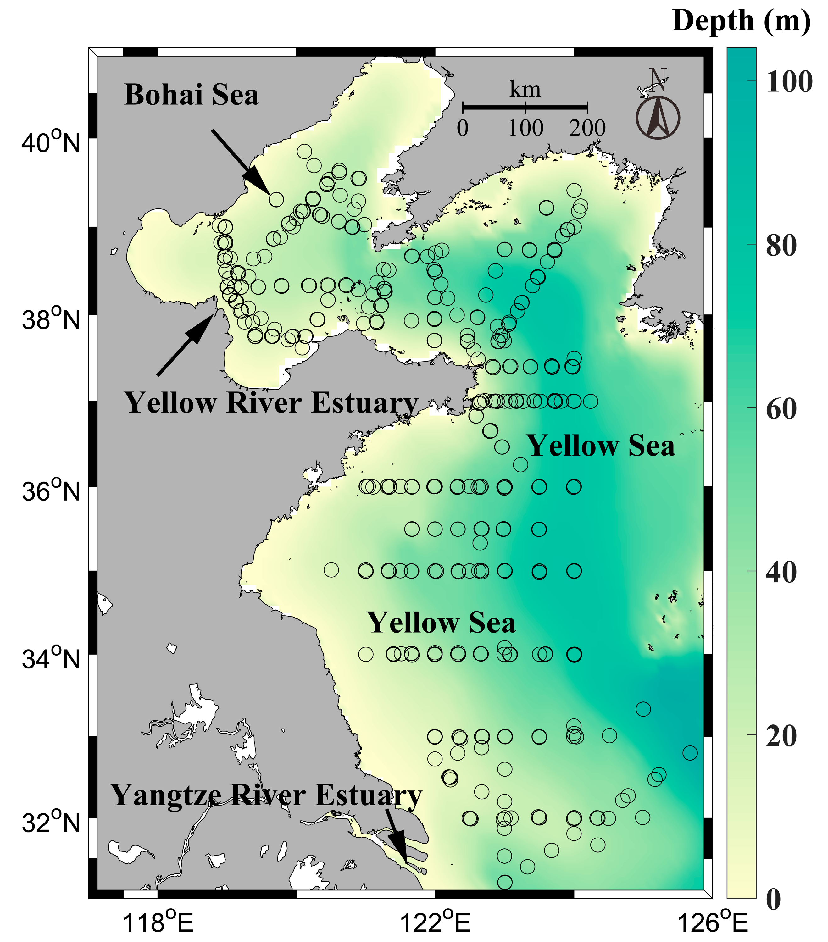
2.1. Study Area
2.2. In Situ Data Measurements
3. Results
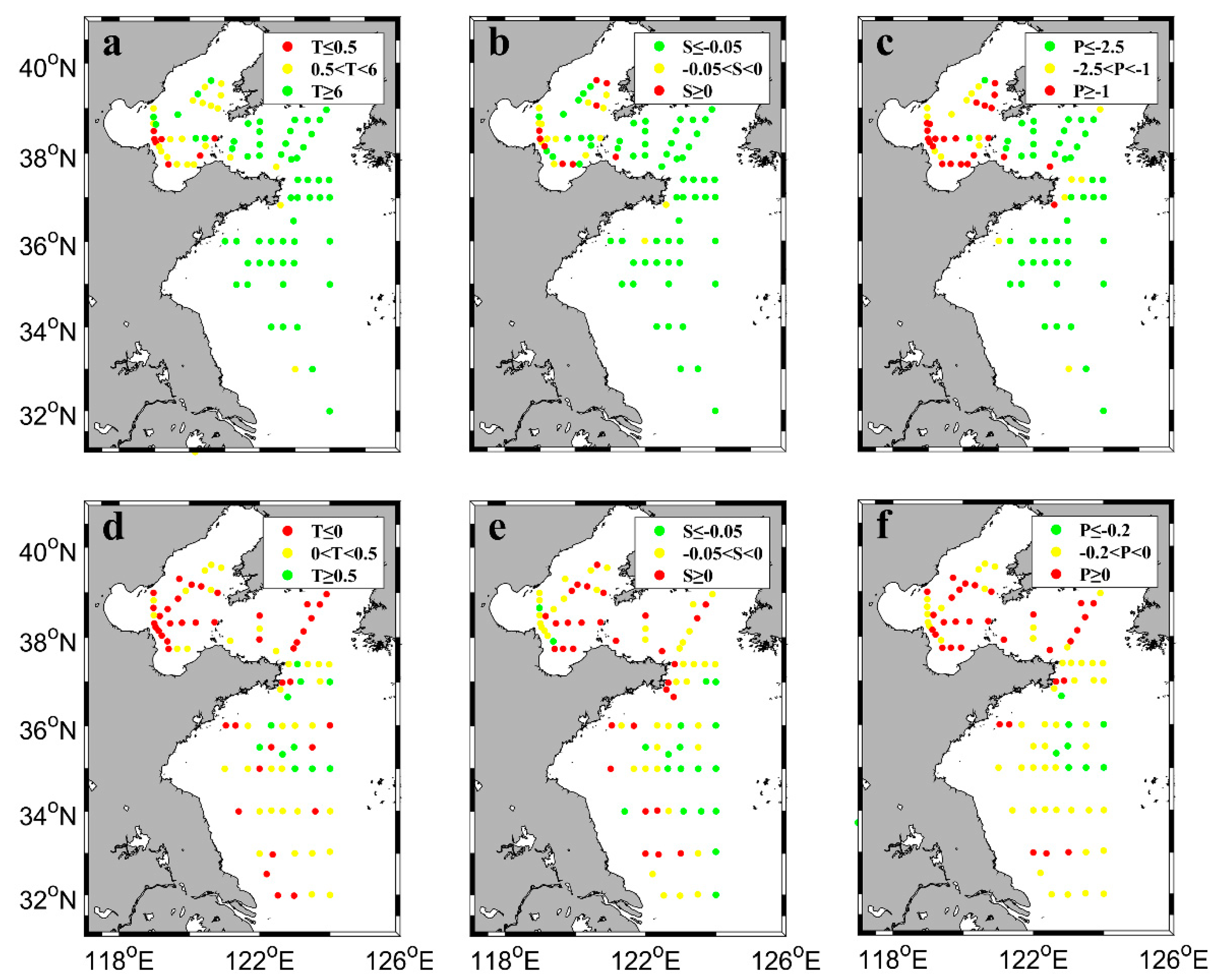
3.1. Hydrography
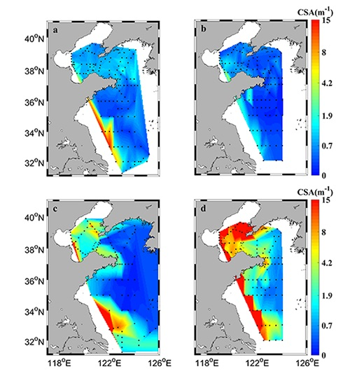
3.2. Horizontal Distribution of CSA
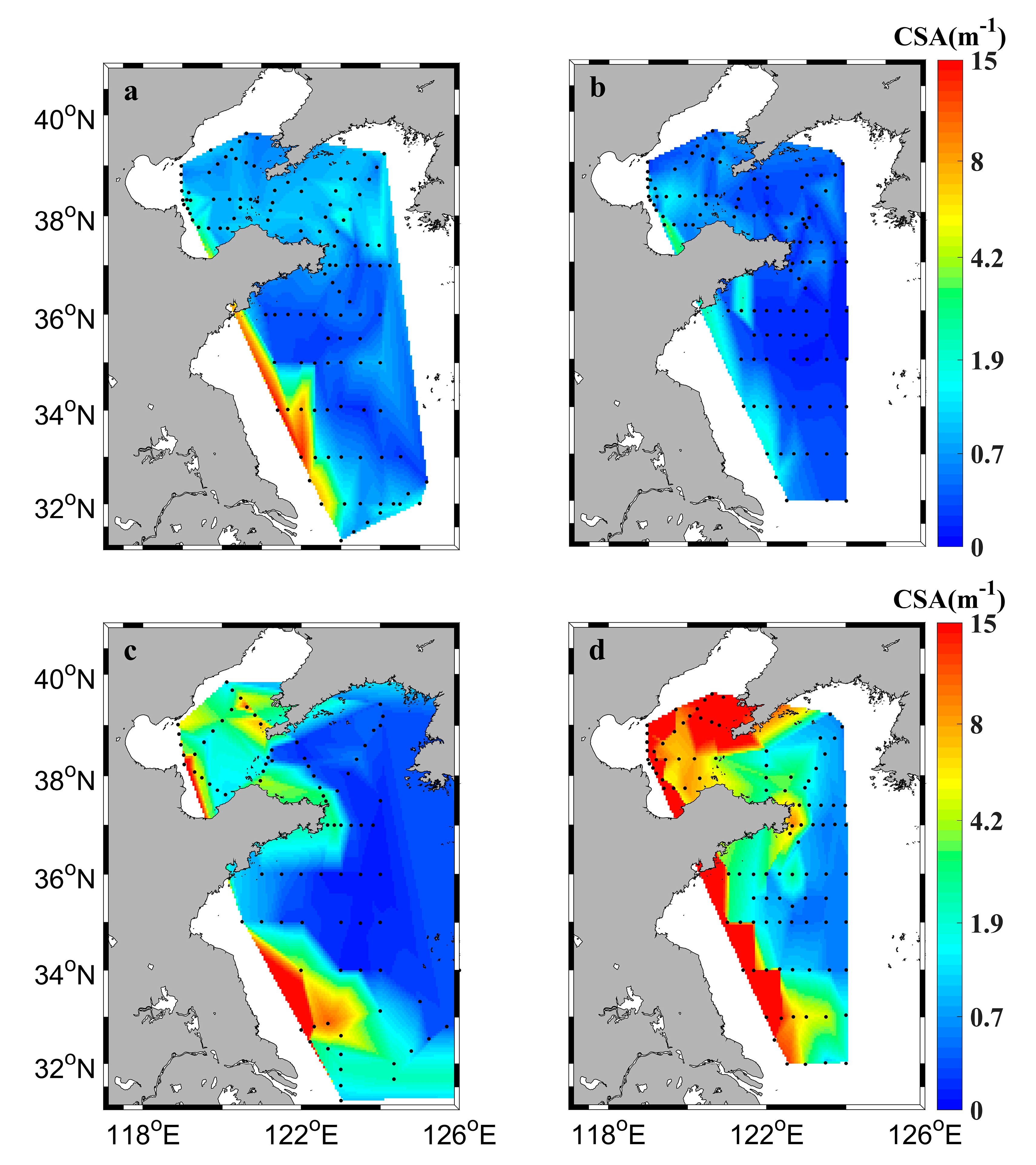
3.3. The Vertical Profiles of CSA
4. Discussion
4.1. Patterns of CSA Variation in the Bohai and Yellow Sea
4.2. Implications of Applications of CSA
5. Conclusions
Author Contributions
Funding
Acknowledgments
Conflicts of Interest
References
- Doxaran, D.; Froidefond, J.M.; Castaing, P.; Babin, M. Dynamics of the turbidity maximum zone in a macrotidal estuary (the Gironde, France): Observations from field and MODIS satellite data. Estuar. Coast. Shelf Sci. 2009, 81, 321–332. [Google Scholar] [CrossRef]
- Soloviev, A.; Lukas, R. The Near-Surface Layer of the Ocean: Structure, Dynamics and Applications; Springer Science & Business Media: Dordrecht, The Netherlands, 2013. [Google Scholar]
- Kara, A.B.; Hurlburt, H.E.; Rochford, P.A.; O’Brien, J.J. The impact of water turbidity on interannual sea surface temperature simulations in a layered global ocean model. J. Phys. Oceanogr. 2004, 34, 345–359. [Google Scholar] [CrossRef]
- Kirk, J.T. Effects of suspensoids (turbidity) on penetration of solar radiation in aquatic ecosystems. Hydrobiologia 1985, 125, 195–208. [Google Scholar] [CrossRef]
- Binding, C.; Bowers, D.; Mitchelson-Jacob, E. Estimating suspended sediment concentrations from ocean colour measurements in moderately turbid waters; the impact of variable particle scattering properties. Remote Sens. Environ. 2005, 94, 373–383. [Google Scholar] [CrossRef]
- Doron, M.; Babin, M.; Hembise, O.; Mangin, A.; Garnesson, P. Ocean transparency from space: Validation of algorithms estimating Secchi depth using MERIS, MODIS and SeaWiFS data. Remote Sens. Environ. 2011, 115, 2986–3001. [Google Scholar] [CrossRef]
- Bowers, D.; Braithwaite, K. Evidence that satellites sense the cross-sectional area of suspended particles in shelf seas and estuaries better than their mass. Geo-Mar. Lett. 2012, 32, 165–171. [Google Scholar] [CrossRef]
- Mobley, C.D. Light and Water: Radiative Transfer in Natural Waters; Academic Press: San Diego, CA, USA, 1994. [Google Scholar]
- Flory, E.; Hill, P.; Milligan, T.; Grant, J. The relationship between floc area and backscatter during a spring phytoplankton bloom. Deep Sea Res. Part I: Oceanogr. Res. 2004, 51, 213–223. [Google Scholar] [CrossRef]
- Neukermans, G.; Loisel, H.; Mériaux, X.; Astoreca, R.; McKee, D. In situ variability of mass-specific beam attenuation and backscattering of marine particles with respect to particle size, density, and composition. Limnol. Oceanogr. 2012, 57, 124–144. [Google Scholar] [CrossRef]
- Mikkelsen, O.A. Variation in the projected surface area of suspended particles: Implications for remote sensing assessment of TSM. Remote Sens. Environ. 2002, 79, 23–29. [Google Scholar] [CrossRef]
- Hatcher, A.; Hill, P.; Grant, J. Optical backscatter of marine flocs. J. Sea Res. 2001, 46, 1–12. [Google Scholar] [CrossRef]
- Brown, C.A.; Huot, Y.; Werdell, P.J.; Gentili, B.; Claustre, H. The origin and global distribution of second order variability in satellite ocean color and its potential applications to algorithm development. Remote Sens. Environ. 2008, 112, 4186–4203. [Google Scholar] [CrossRef]
- Wang, S.; Qiu, Z.; Sun, D.; Shen, X.; Zhang, H. Light beam attenuation and backscattering properties of particles in the Bohai Sea and Yellow Sea with relation to biogeochemical properties. J. Geophys. Res. Oceans 2016, 121, 3955–3969. [Google Scholar] [CrossRef]
- Wang, S.; Huan, Y.; Qiu, Z.; Sun, D.; Zhang, H.; Zheng, L.; Xiao, C. Remote sensing of particle cross-sectional area in the Bohai Sea and Yellow Sea: algorithm development and application implications. Remote Sens. 2016, 8, 841. [Google Scholar] [CrossRef]
- Milligan, T. In situ particle (floc) size measurements with the benthos 373 plankton silhouette camera. J. Sea Res. 1996, 36, 93–100. [Google Scholar] [CrossRef]
- Agrawal, Y.; Pottsmith, H. Instruments for particle size and settling velocity observations in sediment transport. Mar. Geol. 2000, 168, 89–114. [Google Scholar] [CrossRef]
- Sun, D.; Qiu, Z.; Hu, C.; Wang, S.; Wang, L.; Zheng, L.; Peng, T.; He, Y. A hybrid method to estimate suspended particle sizes from satellite measurements over Bohai Sea and Yellow Sea. J. Geophys. Res. Oceans 2016, 121, 6742–6761. [Google Scholar] [CrossRef]
- Zhang, S.; Wang, Q.; Lü, Y.; Cui, H.; Yuan, Y. Observation of the seasonal evolution of the Yellow Sea Cold Water Mass in 1996–1998. Cont. Shelf Res. 2008, 28, 442–457. [Google Scholar] [CrossRef]
- Bian, C.; Jiang, W.; Quan, Q.; Wang, T.; Greatbatch, R.J.; Li, W. Distributions of suspended sediment concentration in the Yellow Sea and the East China Sea based on field surveys during the four seasons of 2011. J. Mar. Syst. 2013, 121, 24–35. [Google Scholar] [CrossRef]
- Morel, A.; Prieur, L. Analysis of variations in ocean color 1. Limnol. Oceanogr. 1977, 22, 709–722. [Google Scholar] [CrossRef]
- Wei, H.; Sun, J.; Moll, A.; Zhao, L. Phytoplankton dynamics in the Bohai Sea—observations and modelling. J. Mar. Syst. 2004, 44, 233–251. [Google Scholar] [CrossRef]
- Fan, H.; Huang, H. Response of coastal marine eco-environment to river fluxes into the sea: A case study of the Huanghe (Yellow) River mouth and adjacent waters. Mar. Environ. Res. 2008, 65, 378–387. [Google Scholar] [CrossRef] [PubMed]
- Zhang, M.; Tang, J.; Song, Q.; Dong, Q. Backscattering ratio variation and its implications for studying particle composition: A case study in Yellow and East China seas. J. Geophys. Res. Oceans 2010, 115, C12. [Google Scholar] [CrossRef]
- Agrawal, Y.; Traykovski, P. Particles in the bottom boundary layer: Concentration and size dynamics through events. J. Geophys. Res. Oceans 2001, 106, 9533–9542. [Google Scholar] [CrossRef]
- Felix, D.; Albayrak, I.; Boes, R.M. Laboratory investigation on measuring suspended sediment by portable laser diffractometer (LISST) focusing on particle shape. Geomar. Lett. 2013, 33, 485–498. [Google Scholar] [CrossRef]
- Traykovski, P.; Latter, R.J.; Irish, J.D. A laboratory evaluation of the laser in situ scattering and transmissometery instrument using natural sediments. Mar. Geol. 1999, 159, 355–367. [Google Scholar] [CrossRef]
- Agrawal, Y.; Whitmire, A.; Mikkelsen, O.A.; Pottsmith, H. Light scattering by random shaped particles and consequences on measuring suspended sediments by laser diffraction. J. Geophys. Res. Oceans 2008, 113, C4. [Google Scholar] [CrossRef]
- Reynolds, R.; Stramski, D.; Wright, V.; Woźniak, S. Measurements and characterization of particle size distributions in coastal waters. J. Geophys. Res. Oceans 2010, 115, C8. [Google Scholar] [CrossRef]
- Sievers, H.A.; Nowlin, W.D., Jr. The stratification and water masses at Drake Passage. J. Geophys. Res. Oceans 1984, 89, 10489–10514. [Google Scholar] [CrossRef]
- Helber, R.W.; Kara, A.B.; Richman, J.G.; Carnes, M.R.; Barron, C.N.; Hurlburt, H.E.; Boyer, T. Temperature versus salinity gradients below the ocean mixed layer. J. Geophys. Res. Oceans 2012, 117, C5. [Google Scholar] [CrossRef]
- Su, J.; Yuan, Y. China Offshore Hydrologica; China Ocean Press: Beijing, China, 2005. [Google Scholar]
- Sun, X. China Offing Sea; China Ocean Press: Beijing, Chnia, 2006. [Google Scholar]
- Bogucki, D.; Dickey, T.; Redekopp, L.G. Sediment resuspension and mixing by resonantly generated internal solitary waves. J. Phys. Oceanogr. 1997, 27, 1181–1196. [Google Scholar] [CrossRef]
- Vangriesheim, A.; Springer, B.; Crassous, P. Temporal variability of near-bottom particle resuspension and dynamics at the Porcupine Abyssal Plain, Northeast Atlantic. Prog. Oceanogr. 2001, 50, 123–145. [Google Scholar] [CrossRef]
- Ladd, C.; Thompson, L.A. Decadal variability of North Pacific central mode water. J. Phys. Oceanogr. 2002, 32, 2870–2881. [Google Scholar] [CrossRef]
- Luo, Y.; Liu, Q.; Rothstein, L.M. Increase of South Pacific eastern subtropical mode water under global warming. Geophys. Res. Lett. 2011, 38, 1. [Google Scholar] [CrossRef]
- Zhang, H.; Qiu, Z.; Sun, D.; Wang, S.; He, Y. Seasonal and interannual variability of satellite-derived chlorophyll-a (2000–2012) in the bohai sea, china. Remote Sens. 2017, 9, 582. [Google Scholar] [CrossRef]
- Gong, X.; Shi, J.; Gao, H. Modeling seasonal variations of subsurface chlorophyll maximum in South China Sea. J. Ocean Univ. China 2014, 13, 561–571. [Google Scholar] [CrossRef]
- Meade, R.H. River-sediment inputs to major deltas. In Sea-Level Rise and Coastal Subsidence; Kluwer: Dordrecht, The Netherlands, 1996; pp. 63–85. [Google Scholar]
- Liu, J.; Xu, K.; Li, A.e.a.; Milliman, J.; Velozzi, D.; Xiao, S.; Yang, Z. Flux and fate of Yangtze River sediment delivered to the East China Sea. Geomorphology 2007, 85, 208–224. [Google Scholar] [CrossRef]
- Gordon, H.R.; Clark, D.K.; Brown, J.W.; Brown, O.B.; Evans, R.H.; Broenkow, W.W. Phytoplankton pigment concentrations in the Middle Atlantic Bight: comparison of ship determinations and CZCS estimates. Appl. Opt. 1983, 22, 20–36. [Google Scholar] [CrossRef] [PubMed]
- Qiu, Z. A simple optical model to estimate suspended particulate matter in Yellow River Estuary. Opt. Express 2013, 21, 27891–27904. [Google Scholar] [CrossRef]
- Qiu, Z.; Su, Y.; Yang, A.; Wang, L.; Mao, Z.; Zhou, B.; Chen, S. An approach for estimating absorption and backscattering coefficients from MERIS in the Bohai Sea. Int. J. Remote Sens. 2014, 35, 8169–8187. [Google Scholar] [CrossRef]
- Smyth, T.J.; Moore, G.F.; Hirata, T.; Aiken, J. Semianalytical model for the derivation of ocean color inherent optical properties: description, implementation, and performance assessment. Appl. Opt. 2006, 45, 8116–8131. [Google Scholar] [CrossRef]
- Bowers, D.; Hill, P.; Braithwaite, K. The effect of particulate organic content on the remote sensing of marine suspended sediments. Remote Sens. Environ. 2014, 144, 172–178. [Google Scholar] [CrossRef]
- Lee, Z.; Carder, K.L.; Arnone, R.A. Deriving inherent optical properties from water color: a multiband quasi-analytical algorithm for optically deep waters. Appl. Opt. 2002, 41, 5755–5772. [Google Scholar] [CrossRef] [PubMed]
- Miller, R.L.; McKee, B.A. Using MODIS Terra 250 m imagery to map concentrations of total suspended matter in coastal waters. Remote Sens. Environ. 2004, 93, 259–266. [Google Scholar] [CrossRef]


© 2019 by the authors. Licensee MDPI, Basel, Switzerland. This article is an open access article distributed under the terms and conditions of the Creative Commons Attribution (CC BY) license (http://creativecommons.org/licenses/by/4.0/).
Share and Cite
Tang, Q.; Wang, S.; Qiu, Z.; Sun, D.; Bilal, M. Variability of the Suspended Particle Cross-Sectional Area in the Bohai Sea and Yellow Sea. Remote Sens. 2019, 11, 1187. https://doi.org/10.3390/rs11101187
Tang Q, Wang S, Qiu Z, Sun D, Bilal M. Variability of the Suspended Particle Cross-Sectional Area in the Bohai Sea and Yellow Sea. Remote Sensing. 2019; 11(10):1187. https://doi.org/10.3390/rs11101187
Chicago/Turabian StyleTang, Qiong, Shengqiang Wang, Zhongfeng Qiu, Deyong Sun, and Muhammad Bilal. 2019. "Variability of the Suspended Particle Cross-Sectional Area in the Bohai Sea and Yellow Sea" Remote Sensing 11, no. 10: 1187. https://doi.org/10.3390/rs11101187
APA StyleTang, Q., Wang, S., Qiu, Z., Sun, D., & Bilal, M. (2019). Variability of the Suspended Particle Cross-Sectional Area in the Bohai Sea and Yellow Sea. Remote Sensing, 11(10), 1187. https://doi.org/10.3390/rs11101187