The Global Spatiotemporal Distribution of the Mid-Tropospheric CO₂ Concentration and Analysis of the Controlling Factors

Abstract

The atmospheric infrared sounder (AIRS) provides a robust and accurate data source to investigate the variability of mid-tropospheric CO₂ globally. In this paper, we use the AIRS CO₂ product and other auxiliary data to survey the spatiotemporal distribution characteristics of mid-tropospheric CO₂ and the controlling factors using linear regression, empirical orthogonal functions (EOFs), geostatistical analysis, and correlation analysis. The results show that areas with low mid-tropospheric CO₂ concentrations (20°S–5°N) (384.2 ppm) are formed as a result of subsidence in the atmosphere, the presence of the Amazon rainforest, and the lack of high CO₂ emission areas. The areas with high mid-tropospheric CO₂ concentrations (30°N–70°N) (382.1 ppm) are formed due to high CO₂ emissions. The global mid-tropospheric CO₂ concentrations increased gradually (the annual average rate of increase in CO₂ concentration is 2.11 ppm/a), with the highest concentration occurring in spring (384.0 ppm) and the lowest value in winter (382.5 ppm). The amplitude of the seasonal variation retrieved from AIRS (average: 1.38 ppm) is consistent with that of comprehensive observation network for trace gases (CONTRAIL), but smaller than the surface ground stations, which is related to altitude and coverage. These results contribute to a comprehensive understanding of the spatiotemporal distribution of mid-tropospheric CO₂ and related mechanisms.

1. Introduction

Since the industrial revolution, as a result of human activity, particularly the combustion of large quantities of fossil fuels and forest destruction, the average global atmospheric CO₂ concentration has increased from pre-industrial revolution level of 280 ppm to 404 ppm in 2017—a 44.3% increase—and has been continuously increasing at a rate of 2.14 ppm/a [1]. A continual increase in atmospheric CO₂ concentrations will alter carbon exchange between the atmosphere and marine and terrestrial ecosystems, and thus cause changes in global temperatures and precipitation, which will have a significant impact on global climate, ecology, and economy. Consequently, this increase has garnered public attention [2,3]. The main atmospheric CO₂ sources and sinks are all distributed in the troposphere. On a monthly average scale, the distribution characteristics of CO₂ sources and sinks on the ground are retained in the horizontal CO₂ concentration gradient in the troposphere. Therefore, to analyze global CO₂ transport and the carbon cycle, examine CO₂ sources and sinks and control CO₂ emissions, it is particularly imperative to accurately acquire tropospheric CO₂ concentration data and study the distribution and variation characteristics of tropospheric CO₂ concentrations [4].

There are two types of sources of common CO₂ data, namely, ground stations and satellites. CO₂ data were measured at ground stations maintained by the World Data Center for Greenhouse Gases (WDCGG) and the total carbon column observing network (TCCON). Although these ground stations have the advantage of generating highly accurate data, the observation methods for ground stations require complex equipment, difficult operations, and high costs, and they lack real-time detection capabilities on a worldwide scale and unified detection methods [5,6,7]. Due to the sparseness and inhomogeneous geographical distribution of ground stations, the spatial and temporal heterogeneity of CO₂ concentration distributions will be neglected when regional and global scale ecological research refers to the global average CO₂ background value of ground stations, which will lead to uncertainty in the research results [2,8]. However, satellite observations with better spatial coverage provide not only stable long-term series observation services worldwide but also three-dimensional information related to atmospheric composition [4,7]. Theoretical studies have shown that satellite data, if sufficiently accurate and precise, have the potential to significantly reduce uncertainties in surface CO₂ fluxes [2,6,9]. As a result, satellite observation data are extremely important for research on the temporal and spatial distributions of CO₂ concentrations as well as CO₂ sources and sinks. Currently, the sensors to observe CO₂ concentrations mainly consist of the atmospheric infrared sounder (AIRS) sensor on the Aqua satellite [10,11], the infrared atmospheric sounding interferometer (IASI) aboard the meteorological operational (Metop)-A satellite [12], the scanning imaging absorption spectrometer for atmospheric chartography (SCIAMACHY) aboard the environmental satellite (ENVISAT) [13,14] and the thermal and near-sensor for carbon observation (TANSO) on the greenhouse gases observing satellite (GOSAT) [15,16]. As the only sensor for monitoring mid-tropospheric CO₂ concentrations, the AIRS sensor has the following unparalleled advantages over other sensors [17,18]: (1) AIRS CO₂ products have higher spatial coverage and are of a longer time series. (2) The AIRS sensor is sensitive to changes in mid-tropospheric CO₂ concentrations and is relatively insignificantly affected by aerosols and clouds. (3) The AIRS sensor has a higher capability to detect atmospheric CO₂ over the oceans. Due to these advantages, many researchers have performed extensive and in-depth studies on mid-tropospheric CO₂ concentrations based on AIRS data. However, most of these studies are focused on retrieval methods for CO₂ concentrations [19,20], data accuracy verification [20,21,22], and the temporal and spatial distribution patterns of CO₂ [4,23,24,25,26]. There are relatively few papers [27,28,29] that quantitatively analyze the factors affecting the temporal and spatial distributions of mid-tropospheric CO₂ concentrations, particularly on a global scale.

In view of the aforementioned problem, in this study, we first verify the accuracy of CO₂ data retrieved from AIRS data obtained from aircraft observations, then analyze the temporal and spatial distribution characteristics of mid-tropospheric CO₂ concentrations using geostatistical, linear regression, and empirical orthogonal function methods, and finally quantitatively analyze the possible factors that affect spatial distribution characteristics through correlation analysis in conjunction with auxiliary data.

2. Materials and Methods

2.1. Data-Sets

Several data-sets are used in this study, including the AIRS L3 CO₂ data product, aircraft and ground-based observation data for atmospheric CO₂ concentration, fossil fuel emission data, and wind field data.

2.1.1. AIRS L3 CO₂ Product

The AIRS, an instrument aboard the Aqua Satellite—an Earth observing system satellite—that was successfully launched in May 2002, is the first new-generation high-spectral resolution infrared sounder with 2378 channels. It measures outgoing radiation in three bands that can retrieve measurements of various atmospheric parameters, including temperature, water vapor profile, and mid-tropospheric CO₂ concentration [10]. The AIRS is the first sensor in the world that retrieves measurements of daily CO₂ concentrations under cloud and cloudless conditions around the globe, including terrestrial, oceanic, and polar regions [30]. AIRS CO₂ data are retrieved using vanishing partial derivatives (VPD) [31]. Considering that the range of 690–725 cm⁻¹ is best for retrieving the CO₂ mixing ratio and the weighting function of the AIRS CO₂ channel peaks between 500 hPa and 300 hPa [32], the mid-troposphere is defined as a layer of atmosphere over the altitude range between 6 and 10 km (between approximately 500 and 300 hPa) [33]. AIRS CO₂ products are provided to the scientific community and the public, free of charge, and can be downloaded from the Goddard Earth Sciences Data and Information Services Center (GES DISC; http://disc.sci.gsfc.nasa.gov/AIRS). Currently, the AIRS data products mainly include the L1B (Level 1B), L2 (Level 2), and L3 (Level 3) data products. The AIRS L1B data products are obtained by subjecting the AIRS L1A data to calibration, positional-parameter analysis, and normalization treatments. The AIRS L2 data products, which are higher-level data products than the L1B data products, are obtained through scientific data processing. Among the AIRS L2 data products are the L2 standard retrieved product, the L2 clear-sky radiation product and the L2 auxiliary data product. The AIRS L3 data products are statistical data for geophysical parameters obtained by subjecting low-level products to temporal and spatial re-sampling and parameter simplification and re-combination treatments. The AIRS L3 data are low in volume and can be directly used without extensive processing. The AIRS L3 data products contain the average value, count and standard deviation at each grid point and include daily (AIRX3C2D), eight-day (AIRX3C28), and monthly (AIRX3C2M) data products. Multi-day products are obtained simply by arithmetically averaging daily data [25]. The AIRS/Aqua Level 3 monthly CO₂ retrieval product (AIRS+AMSU) V005 (AIRX3C2M V5) contains standard retrieval means, standard deviations and input counts, as well as the latitude and longitude arrays giving the centers of the grid boxes. Each file covers a calendar month. The mean values are simply the arithmetic means of the individual CO₂ retrievals that fall within a particular grid box over the month. The mid-tropospheric CO₂ retrievals are averaged and binned into 2.5 × 2 deg grid cells (from −180.0 to +180.0 deg longitude and from −60.0 to +90.0 deg latitude) [34]. In this study, the AIRX3C2M V5 data product for the period from January 2003 to December 2011, was selected to analyze long-term temporal and spatial variations in mid-tropospheric atmospheric CO₂ concentrations. Considering the need for subsequent research, the AIRS CO₂ data product was resampled to 2.5° × 2.5°.

2.1.2. Aircraft and Ground-Based Observation Data

Before using the AIRS CO₂ data product to examine the temporal and spatial distribution characteristics of the mid-tropospheric CO₂ concentration, the accuracy of the AIRS-retrieved CO₂ data product was verified using aircraft observation data that were obtained from the comprehensive observation network for trace gases by airliner (CONTRAIL; http://www.cger.nies.go.jp/contrail/) project and can been download from the WDCGG (https://ds.data.jma.go.jp/gmd/wdcgg/). The CONTRAIL project deploys two types of instruments to measure CO₂ concentrations: Continuous CO₂ measuring equipment (CME) and Automatic air Sampling Equipment (ASE). The CME instrument is installed on eight Boeing 777–200 ER and two Boeing 777–300 ER aircrafts of Japan Airlines (JAL), while the ASE is installed only on the Boeing 747–400 planes that fly twice a month between Australia, Narita, and Sydney to perform flask measurements of CO₂ and other trace gases [35]. The CO₂ mixing ratio is analyzed using a non-dispersive infrared gas analyzer (NDIR; LI-COR, either LI-6252 or LI-6262). At present, the time interval in which the standard gases are introduced into non-dispersive infrared (NDIR) cells is different at different stages of a flight (every 14 minutes during the ascending/descending portion of the flight; every 60 min during the constant altitude portion of the flight, typically at 8–12 km). The data from CME platforms was recorded as 10 s averaged measurements during the ascent/descent (100 m intervals in altitude) and at 1 min intervals during cruising (15 km intervals horizontally). The overall analytical accuracy of the CME is estimated to be <0.2 ppm [36]. The monthly average of aircraft observations for six regions (a, b, c, d, e, and f) for the period from January 2003 to December 2011 are listed in

Table 1. Comparison of mid-tropospheric CO₂ concentrations retrieved from the atmospheric infrared sounder (AIRS) data with aircraft observations made from 2003 to 2011. *** indicates the significance level (p < 0.001).

	Coordinates (°)	Yearly Growth (ppm/a)			Monthly Average (ppm)
		Aircraft	Satellite	Deviation	Aircraft	Satellite	Deviation	R
CONTRAIL a area	20°S–30°S,148°E–155°E	1.85	2.00	0.15	380.8	381.2	0.39	0.99 ***
CONTRAIL b area	10°S–20°S,146°E–154°E	1.90	1.92	0.02	380.9	381.1	0.16	0.98 ***
CONTRAIL c area	0–10°S,142°E–151°E	2.03	2.00	0.03	381.1	381.4	0.30	0.99 ***
CONTRAIL d area	0–10°N,142°E–149°E	1.98	1.92	0.08	381.5	381.9	0.36	0.97 ***
CONTRAIL e area	10°N–20°N,137°E–148°E	1.94	1.92	0.02	381.7	381.6	0.09	0.95 ***
CONTRAIL f area	20°N–30°N,135°E–146°E	1.91	1.87	0.04	381.6	381.5	0.14	0.95 ***
Average		1.93	1.94	0.06	381.3	381.5	0.24

. The deviation refers to the absolute value of the difference between aircraft observations and AIRS.

To compare the seasonal cycle of CO₂ concentration derived from the AIRS product with that derived from the observations, the aircraft observations originating from CONTRAIL (Table 1), and the monthly average data measured at eight background observation stations (Anmyeon-do, Assekrem, Mt. Dodaira, Niwot Ridge, Izaña, Kisai, Mauna Loa, and Yonagunijima) around the globe provided by WDCGG, were selected (

Table 2. Ground station information and comparison of the growth rate of the CO₂ concentration retrieved from AIRS data with ground-based station observations made from 2003–2011.

	Ground Station Information			Yearly Growth (ppm/a)
	GAW Category	Coordinate (°)	Altitude	Ground	Satellite	Deviation
Alert	Global	82.45°N,62.51°W	210	1.95	2.29	0.34
Anmyeon-do	Regional	36.54°N,126.33°E	112	2.11	2.14	0.04
Ascension Island	Regional	7.92°S,14.42°W	54	1.86	2.17	0.31
Assekrem	Global	23.27°N,5.63°E	2710	2.00	2.04	0.05
Barrow	Global	71.32°N,156.61°W	27	1.96	2.32	0.36
Cape Point	Global	34.35°S,18.49°E	260	1.87	2.15	0.28
Mt. Dodaira	Contributing	36°N,139.2°E	860	1.98	2.15	0.17
Niwot Ridge	Regional	40.04°N,105.54°W	3021	1.97	2.16	0.18
Izaña	Global	28.31°N,16.5°W	2381	2.13	2.08	0.05
Kisai	Contributing	36.08°N,139.55°E	33	1.98	2.15	0.17
Mauna Loa	Global	19.54°N,155.58°W	3437	1.98	2.04	0.06
Pallas	Global	67.97°N,24.12°E	567	1.96	2.20	0.23
Plateau Rosa	Regional	45.93°N,7.7°E	3480	1.95	2.08	0.13
Pic du Midi	Contributing	42.94°N,0.14°E	2877	1.97	2.00	0.03
Mt. Waliguan	Global	36.28°N,100.9°E	3890	2.10	2.14	0.05
Wendover	Regional	39.88°N,113.72°W	1320	2.01	2.14	0.12
Yonagunijima	Regional	24.47°N,123.01°E	50	2.00	2.12	0.13
Ryori	Regional	39.03°N,141.82°E	280	1.95	2.17	0.23
Samoa	Global	14.25°S,170.56°W	60	1.92	2.04	0.11
Zugspitze	Global	47.42°N,10.98°E	2656	1.81	2.11	0.30
Average				1.97	2.13	0.17

) for the period from January 2003 to December 2011. To compare the growth rate of CO₂ concentration from AIRS, twenty ground stations (including the eight ground stations listed previously) with fewer missing data from WDCGG were selected (Table 2).

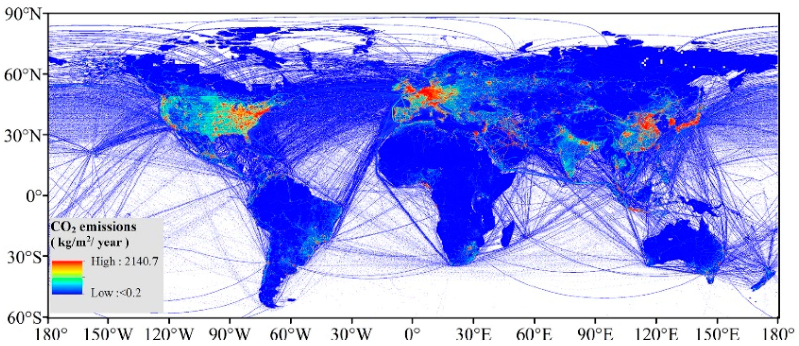
2.1.3. Global Fossil CO₂ Emission Product

The fossil fuel emission data used in this study originated from the emissions database for global atmospheric research (EDGAR)’s global fossil CO₂ emission dataset (EDGAR v4.3.2; https://data.europa.eu/doi/10.2904/JRC_DATASET_EDGAR), which is a global 0.1° × 0.1° spatial grid database for greenhouse gas emissions jointly developed by the Joint Research Centre (JRC) of the European Commission and the Netherlands Environmental Assessment Agency (NEAA) [37]. The anthropogenic CO₂ emission sources used in this study included combustion of fossil fuels and industrial processes (e.g., cement production and the use of carbonates such as limestone and dolomite) but excluded short-term combustion of biomass (e.g., combustion of agricultural waste) and large-scale combustion of biomass (e.g., forest fires).

2.1.4. Wind Field Product

To understand the relationship between the mid-tropospheric CO₂ concentrations and the wind, the zonal components (“u-wind” and “v-wind”; units: “m/s”) and the vertical component (“omega”; units: “Pascal/s”) from the National Centers for Environmental Prediction (NCEP)/National Center for Atmospheric Research (NCAR) re-analysis data were used in this study. The time resolution is one month, and the Geographic Coordinate System-World Geodetic Survey 1984 (GCS-WGS-84) coordinate system was adopted [38]. The above wind data covered the period from 2003 to 2011. These data are a result of global data assimilation carried out collaboratively by the U.S. NCEP and NCAR. The wind field data have a spatial resolution of 2.5° × 2.5°. To represent upward movement with positive values, vertical wind field velocities were multiplied by −1.

2.2. Methodology

A trend analysis of mid-tropospheric atmospheric CO₂ concentrations was performed using a pixel-based linear regression model (the method of least squares (MLS)) and empirical orthogonal function (EOF) decomposition.

The principle of the pixel-based linear regression method is to establish linear functions between the mid-tropospheric CO₂ concentrations in each pixel in research area $x_i$ at the corresponding time $t_i$ for various time series:

$$x_i=a+b{t}_i(i=1,2,\dots ,n),$$

(1)

where $a$ is a regression constant; $b$ is a regression coefficient; and $n$ is the time series number. $b$ and the correlation coefficient, $r$, are calculated using the MLS. When $r$ is significant (p < 0.05) and $b$ is positive, then the mid-tropospheric CO₂ concentration increases significantly within the study period, whereas negative $b$ indicates that the mid-tropospheric CO₂ concentration decreases significantly within the study period. The value of $b$ reflects the rate of increase or decrease in mid-tropospheric CO₂ concentration within the study period.

EOF decomposition is a method for analyzing the structural characteristics of a variable field and extracting its main eigenvalues [39]. This method expresses the characteristics of regional variations by isolating the spatial structural characteristics of the variable field and the corresponding time coefficient [40]. We assumed that the mid-tropospheric CO₂ concentrations have been measured by AIRS at locations $x_1$, $x_2$,…, $x_m$ taken at times $t_1$, $t_2$,…, $t_n$. Mid-tropospheric CO₂ concentrations retrieved from AIRS were stored in a matrix $X$ as $n$ maps each being $m$ points long:

$$X=\left[\begin{array}{cccccc}{x}_{11}& x_{12}& \cdots & x_{1j}& \cdots & x_{1n}\\ x_{21}& x_{22}& \cdots & x_{2j}& \cdots & x_{2n}\\ ⋮& ⋮& ⋮& ⋮& ⋮& ⋮\\ x_{i1}& x_{i2}& \cdots & x_{ij}& \cdots & x_{in}\\ ⋮& ⋮& ⋮& ⋮& ⋮& ⋮\\ x_{m1}& x_{m2}& \cdots & x_{mj}& \cdots & x_{mn}\end{array}\right],$$

(2)

where $m$ is a spatial point, which, in this study, refers to a grid point, and $n$ is time series number. $x_{ij}$ ($i=1,2,\dots ,m$ and $j=1,2,\dots ,n$) represents the $j^{th}$ observation at the $i^{th}$ grid point. Each column of matrix $X$ is one map, and each row of matrix $X$ is a time series of observations for a given location. The EOF expansion of a variable field is the process of decomposing $X$ into the sum of the products of the spatial modes and the time coefficients:

$$x_{ij}={\displaystyle \sum _{k=1}^m{v}_{ik}{t}_{kj}=v_{i1}{t}_{1j}+v_{i2}{t}_{2j}+\cdots +v_{im}{t}_{mj}},$$

(3)

which has the following matrix form:

$$X=VT,$$

(4)

where

$$V=\left[\begin{array}{cccc}{v}_{11}& v_{12}& \cdots & v_{1m}\\ v_{21}& v_{22}& \cdots & v_{2m}\\ ⋮& ⋮& & ⋮\\ v_{m1}& v_{m2}& \cdots & v_{mm}\end{array}\right]$$

(5)

$$T=\left[\begin{array}{cccc}{t}_{11}& t_{12}& \cdots & t_{1n}\\ t_{21}& t_{22}& \cdots & t_{2n}\\ ⋮& ⋮& & ⋮\\ t_{m1}& t_{m2}& \cdots & t_{mn}\end{array}\right]$$

(6)

$V$ is a spatial function matrix that is used to describe the distribution characteristics of a given model, and $T$ is a time coefficient matrix that is used to describe the variation of deviation over time. Based on orthogonality, $V$ and $T$ should satisfy the following conditions:

$$\{\begin{array}{l}{\displaystyle \sum _{i=1}^m{v}_{ik}{v}_{il}=1\left(k=l\right)}\\ {\displaystyle \sum _{j=1}^n{t}_{kj}{t}_{lj}=0\left(k\ne l\right)}\end{array}$$

(7)

which can be written in the following matrix form:

$$V^{T}V=I$$

(8)

$$T{T}^T=\Lambda =\left[\begin{array}{cccc}{\lambda }_1& & & 0\\ & {\lambda }_2& & \\ & & \ddots & \\ 0& & & {\lambda }_m\end{array}\right]$$

(9)

where $I$ is the identity matrix, and $\Lambda$ is a diagonal matrix composed of eigenvalues ${\lambda }_i$ of the real symmetric matrix $X{X}^T$. $V$ can be determined by the eigenvectors $V_R$ of $X{X}^T$:

$$V=X{V}_R$$

(10)

Then, based on Equations (4) and (8), $T$ can be determined as follows:

$$T=V^{T}X$$

(11)

The time coefficient can be determined by Equation (11).

Based on the eigenvalues ${\lambda }_i$, the contribution rate $r_k$ of the $k^{th}$ spatial mode can be determined as follows:

$$r_k=\frac{{\lambda }_k}{{\displaystyle \sum _{i=1}^m{\lambda }_i}}$$

(12)

where $k=1,2,\dots ,p (p<m)$. The spatial mode with a high contribution rate is the main spatial mode (spatial distribution structure) of the variable $X$. The extreme point of a spatial mode reflects the area sensitive to variations in mid-tropospheric CO₂ concentrations in the nine-year period, i.e., as time passes, mid-tropospheric CO₂ concentrations in this area change to the largest extent. The time coefficient is the weight of a spatial mode and describes its temporal variance. The higher the time coefficient is, the more similar the spatial distribution characteristics of the corresponding year are to the spatial mode. To determine whether the EOF obtained by decomposition has a physical meaning, it is necessary to perform a significance test. In this study, the eigenvalue error range method (the North criterion) [41] was used to determine whether the spatial modes obtained by EOF decomposition have a physical meaning.

Compared to the pixel-based linear regression analysis method, the EOF decomposition method takes into consideration the interactions between pixels and describes the temporal variation characteristics of atmospheric CO₂ concentrations in the area. However, this method is unable to provide the absolute values of variations in mid-tropospheric CO₂ concentrations in pixels. Therefore, the pixel-based linear regression analysis method and the EOF decomposition were used in combination in this study to, not only validate one another, but also make use of each method’s advantages.

The correlation analysis method was employed to analyze the effects of the aforementioned human and natural factors on the spatial distribution of mid-tropospheric CO₂ concentrations (Equation (13)).

$$\mathrm{R}=\frac{{\displaystyle {\sum }_{i=1}^n\left(x_i-\overline{x}\right)}\left(y_i-\overline{y}\right)}{\sqrt{{\displaystyle {\sum }_{i=1}^n{\left(x_i-\overline{x}\right)}^2}}\sqrt{{\displaystyle {\sum }_{i=1}^n{\left(y_i-\overline{y}\right)}^2}}}$$

(13)

where $X$ and $Y$ are two vectors with sample values of $x_i$ and $y_i$ ($i=1,2,\dots ,n$), respectively, and with average values of $\overline{x}$ and $\overline{y}$, respectively.

3. Results

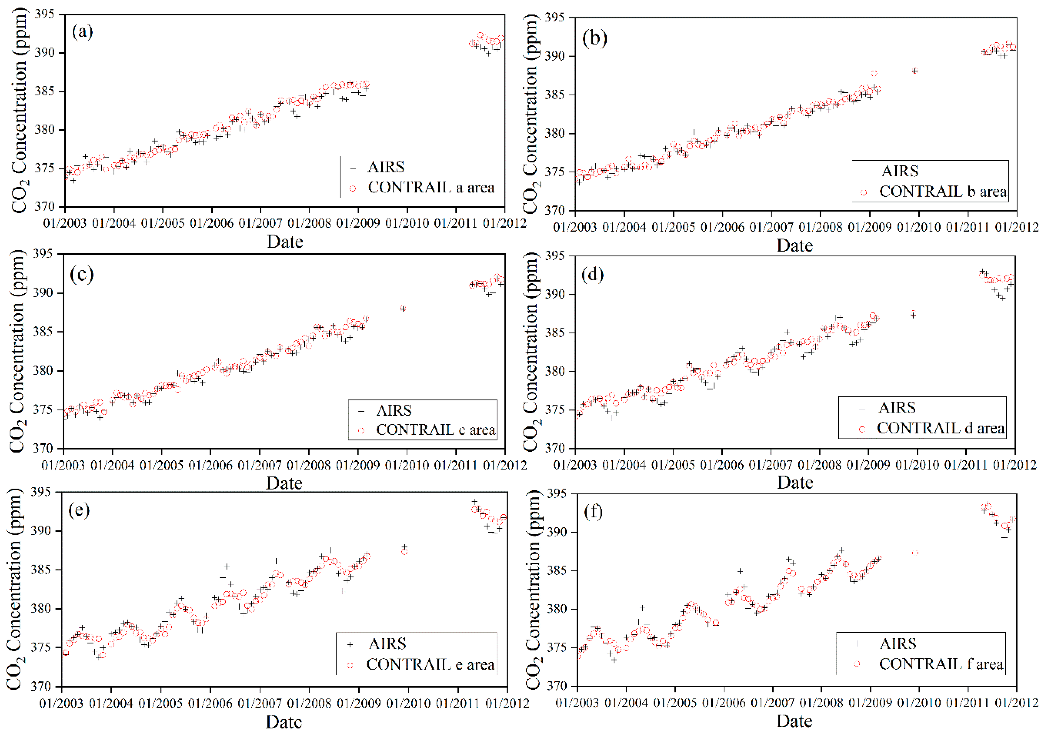
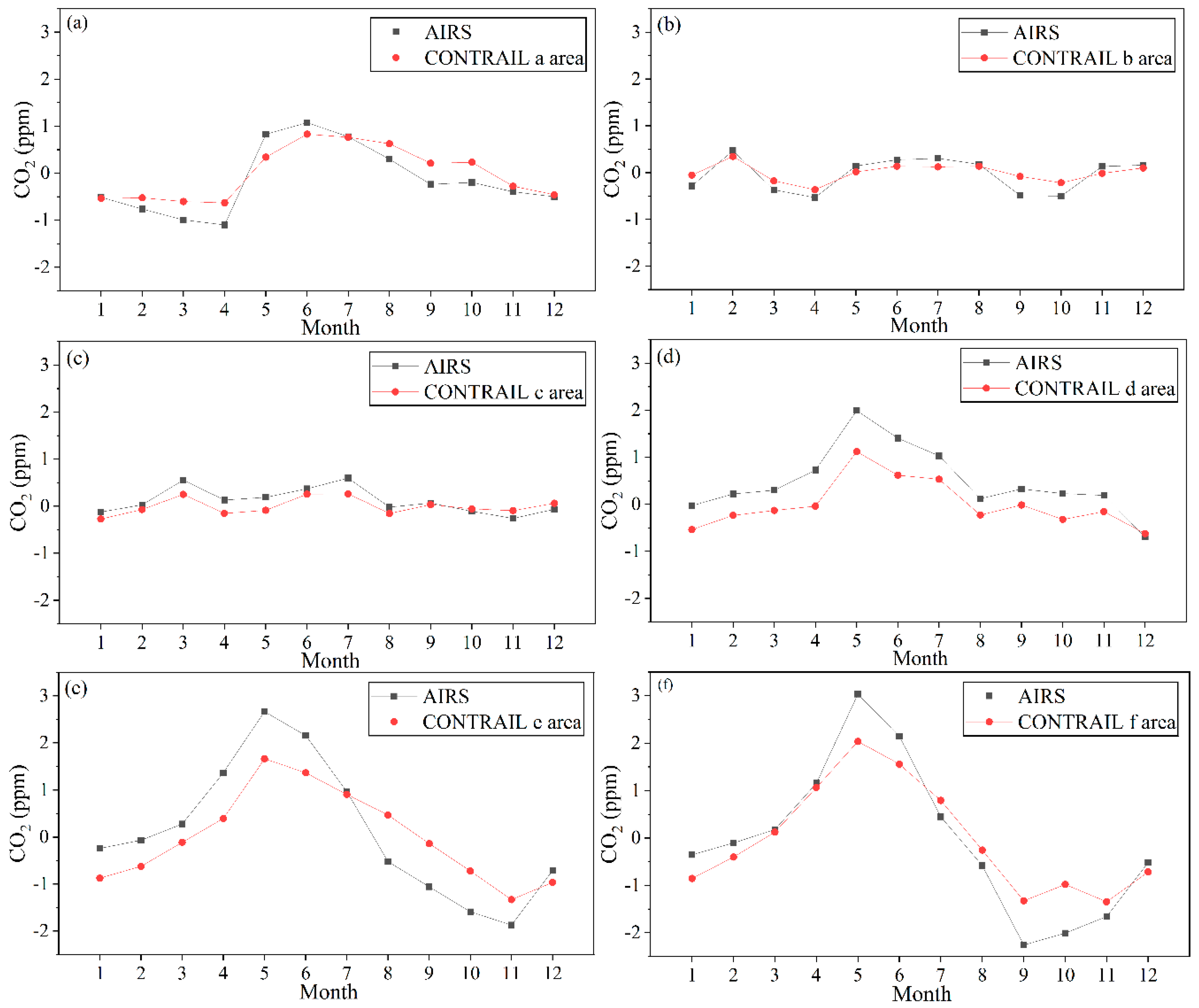
3.1. Aircraft Observation Validation of the AIRS CO₂ Product

The AIRS-retrieved data product was validated using airborne platform observations for the six regions in the CONTRAIL program. We only chose months when both aircraft observations and the AIRS product were available. As demonstrated in Figure 1, the increasing trend of the observed monthly average CO₂ concentrations in each of the six regions in the CONTRAIL program is consistent with that of the corresponding AIRS-retrieved monthly average CO₂ concentration. In addition, both the observed and AIRS-retrieved values display consistent seasonal fluctuations. The statistical results shown in Table 1 demonstrate that the observed monthly average CO₂ concentrations, in the six regions, are highly consistent with the corresponding AIRS-retrieved values. For each of the six regions, the correlation coefficient exceeds 0.94 and passes the significance test at the 0.001 level. In addition, for each of the six regions, the difference between the observed and AIRS-retrieved monthly average CO₂ concentrations is less than 0.4 ppm, and the observed and AIRS-retrieved annual average rates of increase in CO₂ concentration are basically the same, with a difference of only 0.06 ppm/a.

The AIRS-retrieved mid-tropospheric atmospheric CO₂ concentrations are highly consistent with aircraft observations made over the oceans in various latitude zones. In addition, the observed and AIRS-retrieved mid-tropospheric atmospheric CO₂ concentrations display consistent seasonal variations. The average seasonal fluctuation in CO₂ concentrations is approximately 5 ppm [31]. This demonstrates that the AIRS-retrieved data can be used to determine the characteristics of seasonal fluctuations in CO₂ concentrations. In terms of the annual average rate of increase, overall, the AIRS-retrieved annual average rate of increase in mid-tropospheric CO₂ concentration is 1.94 ppm/a, and the observed annual average rate of increase is 1.93 ppm/a. The average of the absolute values of the difference between the AIRS-retrieved and observed values is only 0.06 ppm/a, which indicates that the AIRS-retrieved data can very well reflect the inter-annual variation pattern of mid-tropospheric CO₂ concentrations. Rayner et al. [8] found that a CO₂ concentration accuracy better than 1% (an error less than 4 ppm) could help reduce uncertainties in estimates of CO₂ sources and sinks.

In summary, AIRS-retrieved mid-tropospheric CO₂ concentration data have high accuracy and stability and can be used to analyze the temporal and spatial distribution characteristics of mid-tropospheric CO₂ concentrations.

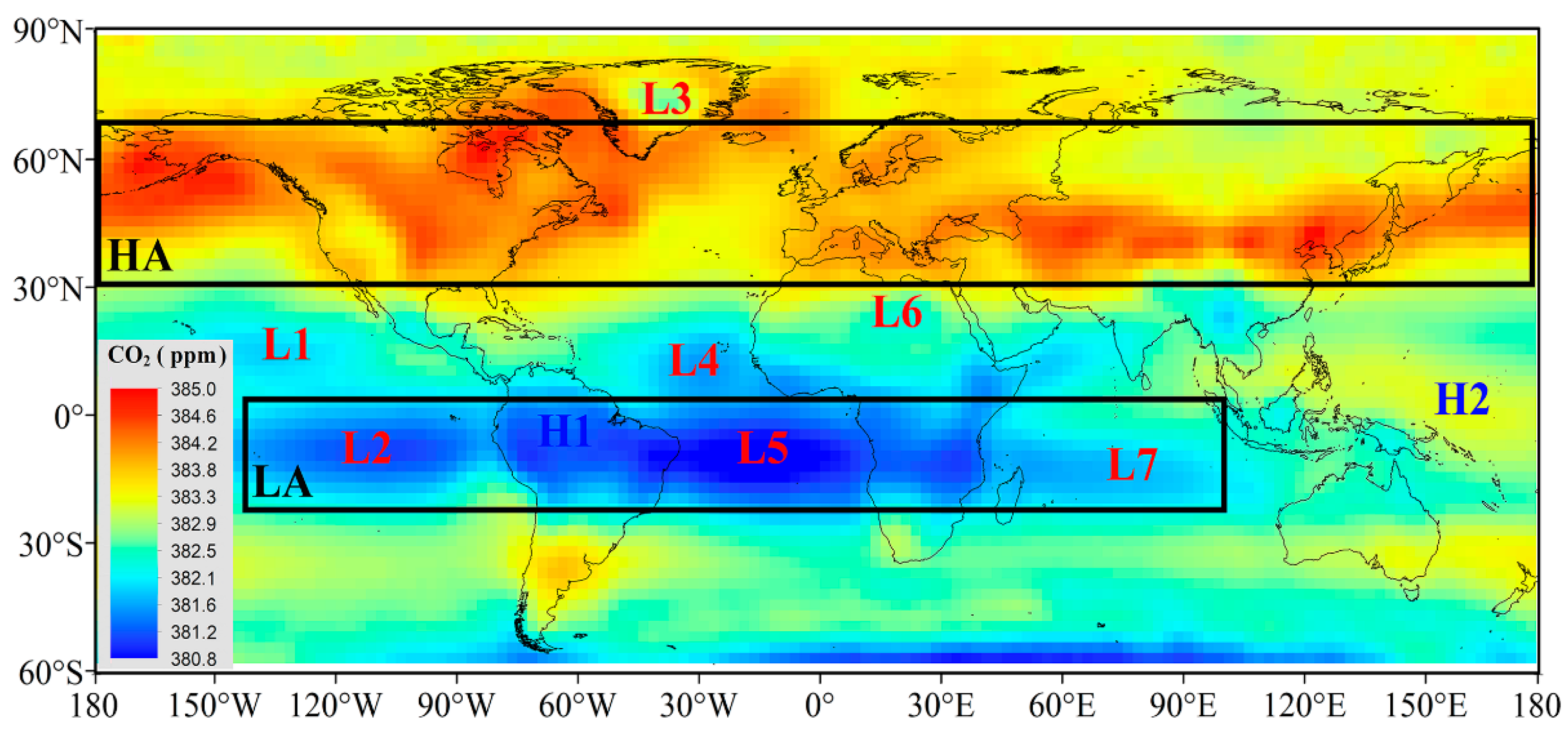
3.2. Spatial Distributions of the Mid-Tropospheric CO₂ Concentration of the World

Figure 2 shows the spatial distribution of AIRS-retrieved global multi-year (January 2003 through December 2011) annual average mid-tropospheric CO₂ concentrations. As demonstrated in Figure 2, the distribution of mid-tropospheric CO₂ concentrations displays notable spatial heterogeneity. Overall, CO₂ concentrations are significantly higher in the Northern Hemisphere (NH) than the Southern Hemisphere (SH), and significantly higher over land than over the oceans, forming a high-low-high spatial distribution pattern. The high-value areas are mostly concentrated between 30°N and 70°N (mean: 384.2 ppm) over northern China, Europe, southeastern Canada, the western U.S., and Alaska and its nearby waters, thus forming a high-latitude high-CO₂ concentration zone in the NH (HA). The Atlantic area between 20°S and 5°N is the global low-CO₂ concentration center (mean: 382.1 ppm), which extends eastward to central-southern Africa and westward to the Pacific west of South America, thus forming a low-CO₂ concentration zone (LA). The mid-tropospheric CO₂ concentration of the Amazon forest region (H1) is higher than that in the surrounding sea area (L2, L5). The mid-tropospheric CO₂ concentration in the western Pacific (H2) is higher than that in the eastern Pacific (L2) at the same latitude. In the L1-L7 region, low value centers, which are distinct from each other and significantly different from the surrounding concentrations, are formed.

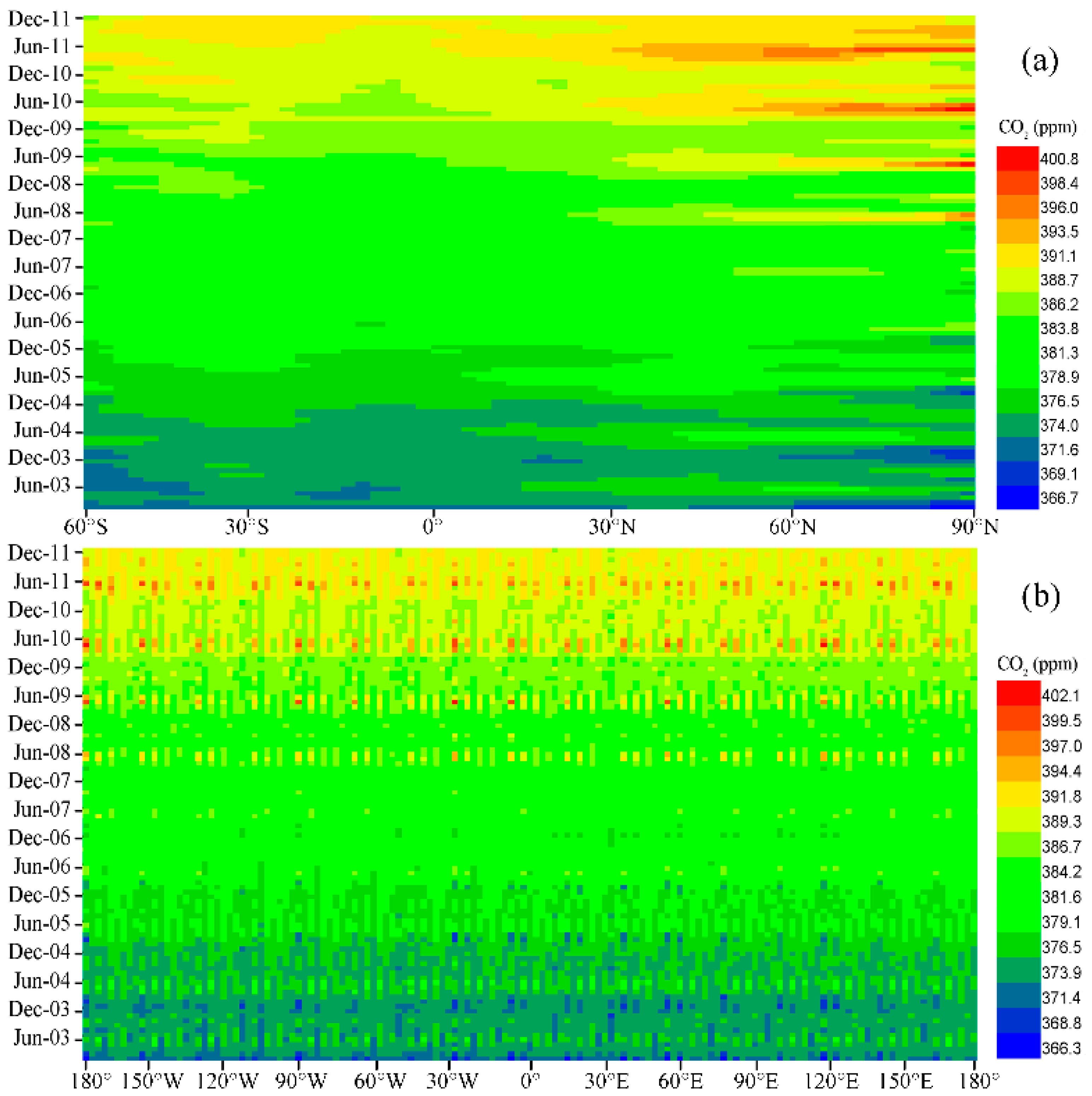
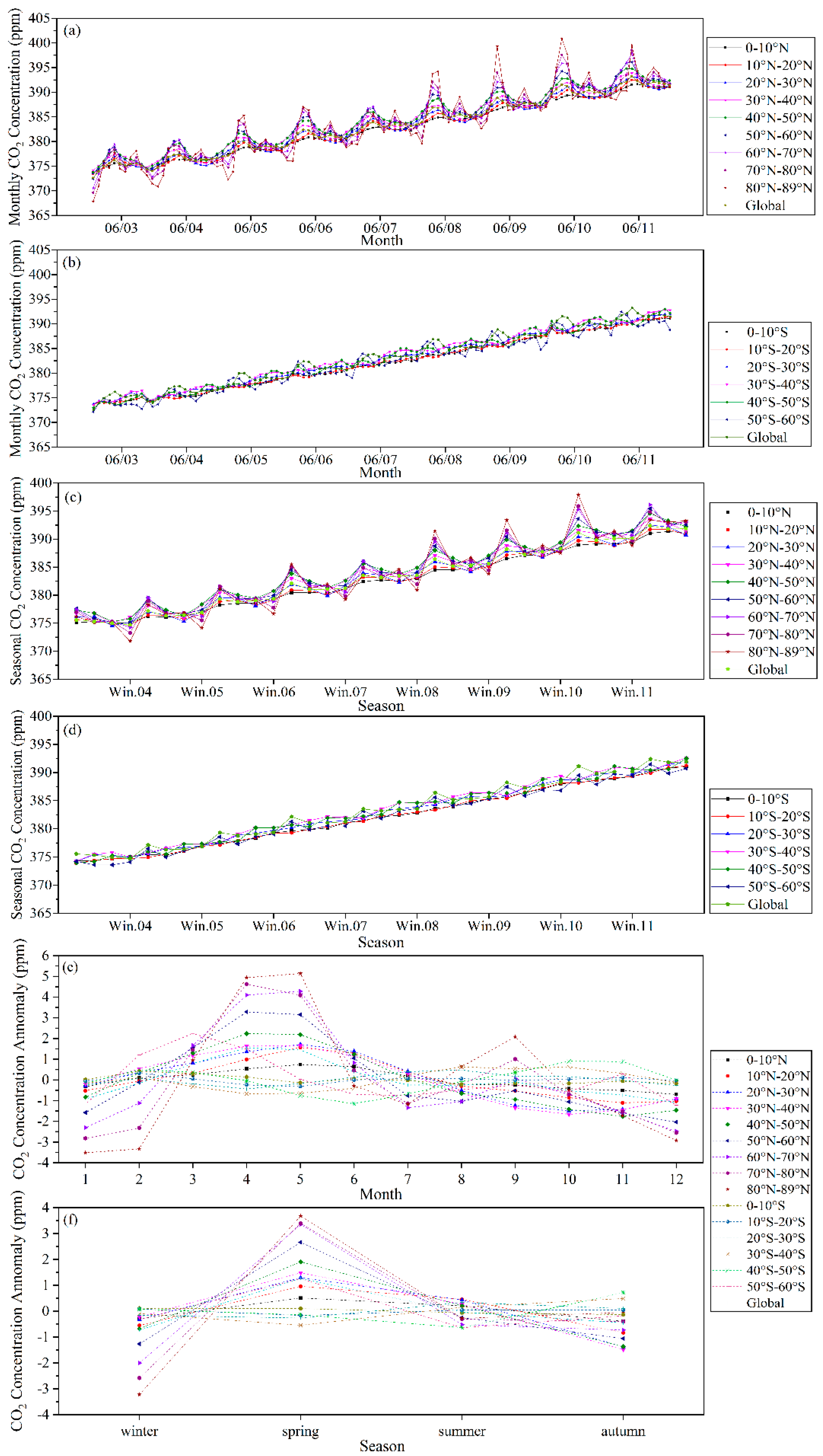
3.3. Temporal Distributions of the Mid-Tropospheric CO₂ Concentration of the World

The pixel-based linear trend analysis (Figure 3a) shows an increase in CO₂ concentration in all the regions around the globe. The rates of increase in CO₂ concentration are significantly higher in the NH than the SH and higher over land than over the oceans. CO₂ concentrations increase relatively rapidly (up to 2.63 ppm/a) in the troposphere over northern Canada above 60°N, central and eastern Russia and the Arctic region and increase relatively slowly (down to 1.96 ppm/a) between 15°N and 15°S over the central and western Pacific.

The EOF analysis of CO₂ concentration shows that the variance contribution rate of the first-order mode is 95% and has passed the eigen-root error range test. Therefore, the first-order mode can represent the spatial structure of variations in mid-tropospheric CO₂ concentrations between 2003 and 2011. The spatial mode of the first-order mode is extremely similar to the spatial variation in CO₂ concentrations obtained by the pixel-based linear trend analysis (Figure 3b). The corresponding time coefficient reflects the temporal variation—continual increase—in this spatial mode.

Table 2 show that the AIRS-retrieved annual average rate of increase in mid-tropospheric CO₂ concentration is 2.13 ppm/a, and the observed annual average rate of increase is 1.97 ppm/a. The average of the absolute values of the difference between the AIRS-retrieved and observed values is 0.17 ppm/a. At the same time, we also find that the rate of increase in the annual average CO₂ concentration calculated from the AIRS CO₂ product is always larger than that calculated from ground stations.

To investigate the temporal and spatial distribution characteristics of CO₂ concentrations in the meridional and zonal directions, the average CO₂ concentrations in these two directions were statistically analyzed and heat maps were produced, as shown in Figure 4. The average value of the difference between adjacent pixels in latitude (0.03 ppm) is roughly ten times than that in longitude. As demonstrated in Figure 4, CO₂ concentrations display notable spatial heterogeneity in the zonal direction (Figure 4a) but no spatial heterogeneity in the meridional direction (Figure 4b).

To further examine the temporal and spatial distribution characteristics of CO₂ concentrations in the zonal direction, the average CO₂ concentrations within every 10° in the zonal direction were calculated, and the results were statistically analyzed.

Table 3. The seasonal and annual mid-tropospheric CO₂ concentration variations in different regions around the world from 2003 to 2011.

	Yearly Average (ppm)	Annual Growth (ppm/a)	Seasonal Average (ppm)				Seasonal Fluctuation (ppm)
			Spring	Summer	Autumn	Winter	Average	Maximum	Minimum
0–10°N	382.5	2.00	382.6	382.8	382.8	382.3	0.54	1.60	0.02
10°N–20°N	382.7	2.01	383.2	383.2	382.5	382.1	0.89	2.25	0.02
20°N–30°N	383.1	2.04	383.9	383.6	382.3	382.9	1.29	2.28	0.04
30°N–40°N	383.9	2.08	384.9	384.2	383.0	383.8	1.44	2.39	0.02
40°N–50°N	384.3	2.13	385.8	384.6	383.6	383.8	1.60	3.29	0.49
50°N–60°N	384.2	2.20	386.4	384.0	383.8	383.1	1.83	5.17	0.07
60°N–70°N	384.0	2.27	386.9	383.6	383.9	382.2	2.50	7.40	0.09
70°N–80°N	383.8	2.26	386.7	383.5	384.0	381.3	2.88	8.21	0.10
80°N–89°N	383.6	2.27	386.8	383.4	384.2	380.4	3.59	10.52	0.07
0–10°S	382.1	2.01	381.8	382.2	382.6	382.2	0.50	1.10	0.11
10°S–20°S	382.1	2.03	381.5	382.2	382.8	382.2	0.51	1.05	0.00
20°S–30°S	382.8	2.03	382.1	383.2	383.5	382.7	0.55	1.48	0.04
30°S–40°S	383.2	2.07	382.2	383.4	384.3	383.2	0.70	1.63	0.02
40°S–50°S	382.9	2.11	382.3	382.3	384.2	383.1	0.69	2.48	0.01
50°S–60°S	382.3	2.08	383.1	381.7	382.7	382.0	1.25	2.70	0.00
NH (0–60°N)	383.6	2.14	385.2	383.7	383.3	382.4	1.84	4.79	0.10
SH (0–60°S)	382.6	2.06	382.2	382.5	383.3	382.6	0.70	2.70	0.00
Global (89°N–60°S)	383.2	2.11	384.0	383.2	383.3	382.5	1.38	10.52	0.00

shows the results.

Of the 15 areas, the annual average CO₂ concentration is the highest (384.3 ppm) in the area between 40°N and 50°N, and lowest (382.1 ppm) between 10°S and 20°S. The annual average rate of increase in CO₂ concentration in the area between 80°N and 90°N is the highest (2.27 ppm/a) and higher by 13.4% than that in the area (between 0 and 10°N) with the lowest annual average rate of increase. Both the annual average mid-tropospheric CO₂ concentrations and annual rates of increase in CO₂ concentration are higher in the NH than the SH. Except for the area between 40°S and 50°S, in which the annual average rate of increase in CO₂ concentration (2.11 ppm/a) is slightly higher than that (2.08 ppm) in the area between 50°S and 60°S, the higher the latitude is, the higher the annual rate of increase is.

Globally, in regard to seasonal and monthly variations, mid-tropospheric CO₂ concentrations display notable seasonal and monthly periodic characteristics (Figure 5). As shown in Figure 5a,b, the mid-tropospheric CO₂ concentrations in each month in all the areas are higher than those in the same month of the previous year. In regard to seasonal variations (Figure 5c,d), except for the areas between 70°N and 80°N and between 80°N and 89°N, the CO₂ concentrations in each season in all the areas are higher than those in the same season of the previous year. This reflects the fact that the atmospheric CO₂ concentrations are continuously on the rise.

To analyze the seasonal variation of mid-tropospheric CO₂ concentrations, the AIRS CO₂ product was de-trended using a linear fitting method. Regarding monthly variability of the de-trended mid-tropospheric CO₂ concentration averaged globally (Figure 5e), the highest mid-tropospheric CO₂ concentration anomaly occurs in April, while the lowest mid-tropospheric CO₂ concentration anomaly occurs in December. In the NH, the highest mid-tropospheric CO₂ concentration anomaly occurs in April (40°N–80°N) or May (0–40°N, 80°N–89°N) and the lowest mid-tropospheric CO₂ concentration anomaly occurs in October (20°N–40°N), November (10°N–20°N, 40°N–50°N), and December (0–10°N, 50°N–70°N). In the SH, the monthly variability of the de-trended mid-tropospheric CO₂ concentration is irregular. Regarding seasonal variability of the de-trended mid-tropospheric CO₂ concentration averaged globally (Figure 5f), mid-tropospheric CO₂ concentrations are the highest in spring (March through May) and lowest in winter (December through to February of the following year). In the NH, the highest mid-tropospheric CO₂ concentrations occur in spring in all areas and the lowest mid-tropospheric CO₂ concentrations occur in fall (September through November) (0–50°N) or winter (50°N–89°N). In the SH, the seasonal variability of the detrended mid-tropospheric CO₂ concentration is irregular as well. The seasonal variations in mid-tropospheric CO₂ are affected by the terrestrial ecosystem [42], rainfall [28,43], wind [27], temperature [29] and CO₂ emission [44].

In regard to the extent of seasonal fluctuations, Figure 5 also shows that the higher the latitude is, the larger the extent of inter-seasonal fluctuations is. Compared to the SH (largest seasonal fluctuation: 2.70 ppm), seasonal fluctuations in the NH (largest seasonal fluctuation: 4.79 ppm) are more intense. The largest seasonal fluctuation occurs between winter and spring, and the smallest seasonal fluctuation occurs between summer and fall. Globally, the average fluctuation between consecutive seasons is 1.38 ppm. The seasonal fluctuation in the area between 80°N and 89°N is the largest (3.59 ppm) and is 6.23 times that in the area between 0 and 10°N (Table 3).

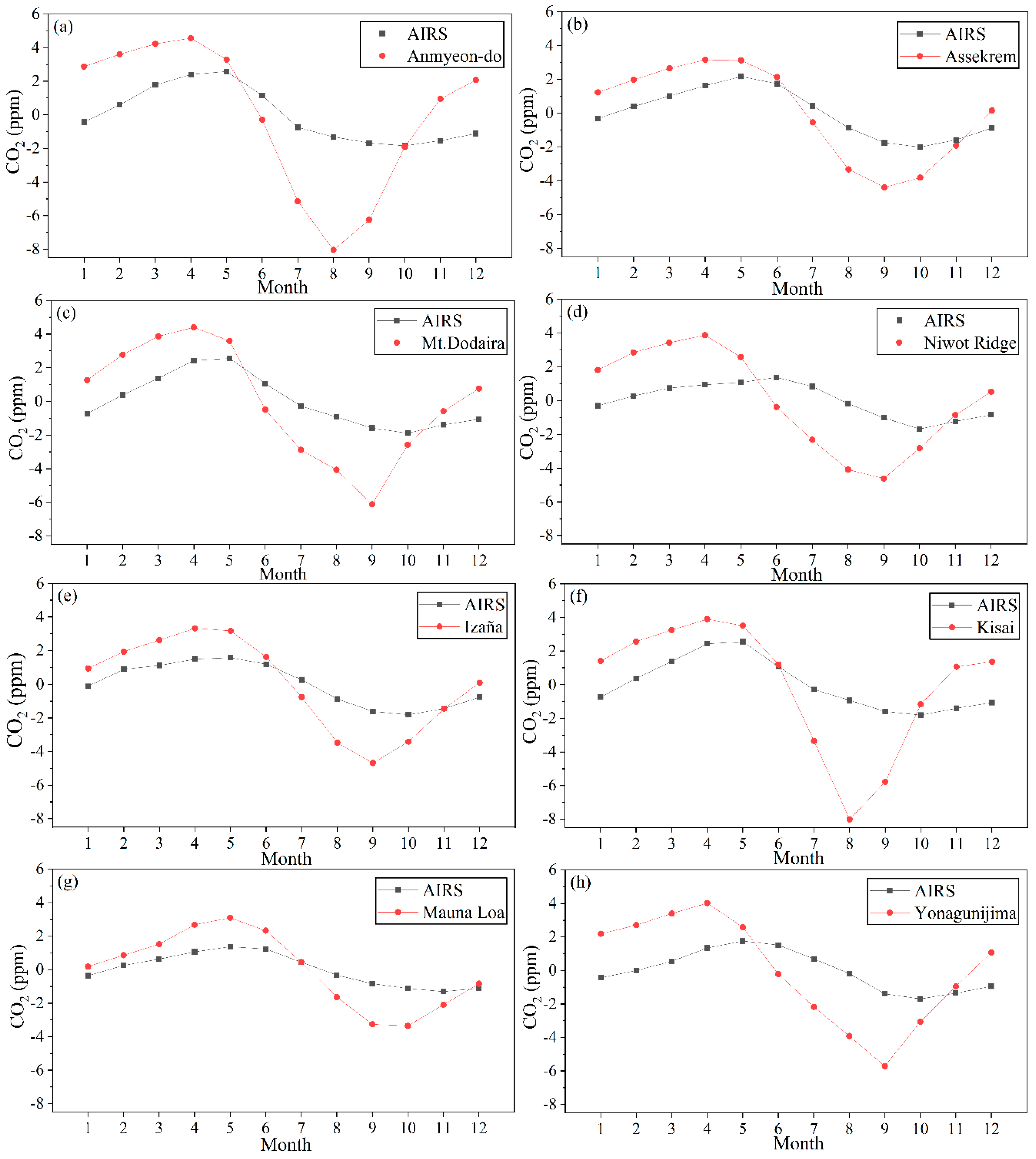
3.4. Comparison of Seasonal Cycles of CO₂ Concentration Derived from AIRS Data with that Derived from Observations

The values of the mid-tropospheric CO₂ concentration derived from the AIRS product were extracted at the point or area where the observations are located and were then de-trended along with observations for the period 2003–2011.

As seen in Figure 6, compared to surface measurements, the amplitude of seasonal variation retrieved from AIRS is lower. This may be related to altitude and coverage. On the one hand, the heights of the stations are less than 4 km and thus greatly affected by the carbon emission and absorption of the underlying surface; CO₂ was retrieved by AIRS at the height of 6-10 km, at which CO₂ is fully mixed. On the other hand, the observed values were obtained from the location of the station, while the CO₂ concentration retrieved from AIRS is the average of the grid (2.5° × 2.5°). In addition, the AIRS mid-tropospheric product lags behind the ground observations. This lag is likely due to the vertical transport of CO₂ [4,12].

The seasonal cycles of CO₂ measured by CONTRAIL and retrieved from AIRS are plotted in Figure 7. There is good agreement between both datasets in terms of cycle amplitude, which increases slightly with latitude. However, the amplitude of CO₂ seasonal fluctuation retrieved from AIRS is larger than that calculated from CONTRAIL, likely due to altitude (CONTRAIL: 812 km; AIRS: 6–10 km).

4. Discussion

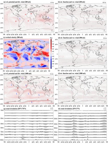
4.1. Effects of Atmospheric Circulations and Carbon Emissions on the Yearly Spatial Distributions of Mid-Tropospheric CO₂ Concentrations

The distribution of mid-tropospheric atmospheric CO₂ concentrations displays notable spatial heterogeneity (Figure 2). This spatial distribution is related to large-scale climate drivers. Kumar et al. [27] noted that upward (downward) winds cause vertical transport of CO₂ from the surface (mid-troposphere) up (down) to the mid-troposphere (surface). However, only the value of vertical velocity at the surface level is considered. In this study, we examine the effects of atmospheric circulations and carbon emissions from ground sources on the spatial distribution of mid-tropospheric atmospheric CO₂ concentrations.

Horizontal wind velocity can be decomposed into a non-divergent (rotational) part and a divergent (irrotational) part. Non-divergent wind vectors are related to horizontal movements. Divergent wind vectors are directly linked to vertical movements [45,46]. A non-divergent wind vector is represented by a stream function. A divergent wind vector is represented by a velocity potential. The low (high) center of a velocity potential is related to a divergent outflow (convergent in-flow). A velocity potential drives the vertical movements of the atmosphere. Divergent winds and vertical movements of the atmosphere are used to characterize atmospheric circulation [47].

In this study, the 200-mb, 500-mb, and 1000-mb levels were selected to represent the upper, mid-, and lower troposphere, respectively. In addition, the horizontal wind fields in the upper and lower troposphere were selected to calculate and plot the divergent wind fields and velocity potentials in the upper and lower troposphere between 2003 and 2011, respectively (Figure 8a,e). The vertical wind field in the mid-troposphere was selected to plot the vertical wind field in the mid-troposphere between 2003 and 2011 (Figure 8c). The horizontal wind fields in the upper, mid-, and lower troposphere were selected to calculate and plot, non-divergent wind fields and stream functions (Figure 8b,d,f). The horizontal and vertical wind fields below the 100–1000-mb levels were selected to calculate and plot the zonal circulations between 30°N and 70°N and between 20°S and 5°N (Figure 8g,h).

As demonstrated in Figure 8, in the L1–L7 regions, there is a divergent outflow from the lower troposphere (Figure 8e), a convergent inflow into the upper troposphere (Figure 8a), and a corresponding vertical downward movement in the mid-troposphere (Figure 8c). It can be inferred that the air currents at the height at which CO₂ is observed in the AIRS data move downward, causing CO₂ to flow from low concentrations to high concentrations. Therefore, in these regions, CO₂ concentrations are lower in the mid-troposphere than the nearby zones. As the two main heat sources in the world [48], the situation in the H1 and H2 regions is just the opposite. Due to the presence of the Amazon rainforest, a strong carbon sink [49], near-surface atmospheric CO₂ concentrations in the H1 region are relatively low, which is reflected by the relatively low mid-tropospheric CO₂ concentrations.

As demonstrated in Figure 9, high-near-surface CO₂ emission areas are mainly concentrated in central and eastern U.S., Europe, northern India, central, and eastern coastal China, South Korea, and Japan. A comparison shows a relatively dispersed distribution of high-near-surface CO₂ emission areas and a relatively continuous distribution of high-mid-tropospheric CO₂ concentration areas. While there is no strict corresponding relationship between the distribution of high-near-surface CO₂ emission areas and the distribution of high-mid-tropospheric CO₂ concentration areas, the regions where high-near-surface CO₂ emission areas are located are also home to high-mid-tropospheric CO₂ concentration areas, but not vice versa. The regions where low-mid-tropospheric CO₂ concentration areas are located are not home to global low-CO₂ emission areas. The formation mechanism of low- and high-mid-tropospheric CO₂ concentration areas cannot be completely explained solely with near-surface CO₂ emissions, but can be clarified when atmospheric circulation is also taken into consideration.

Regarding its horizontal movements, the wind field in the lower troposphere has a relatively low velocity and undergoes notable rotational movements. These movements occur inside the low- and high-mid-tropospheric CO₂ concentration areas. There are no wind movements that connect the high-value areas to the low-value areas. In the high-CO₂ emission areas, winds basically blow from west to east (Figure 8f). In the mid-troposphere, the wind field does not rotate noticeably. In the high-CO₂ emission areas, winds blow from west to east at relatively high velocities (Figure 8d). A similar phenomenon can be found in the upper troposphere (Figure 8b).

The vertical movements of the wind field in the low-mid-tropospheric CO₂ concentration areas (20°S–5°N) and high-mid-tropospheric CO₂ concentration areas (30°N–70°N) are analyzed by assessing the zonal circulations. Between 20°S and 5°N, the atmospheric circulation is relatively deep. The air ascends over the western Pacific, disperses eastward aloft, sinks over the eastern Pacific and returns towards the west (Figure 8h). Within this region, another atmospheric circulation occurs in which air ascends over the Amazon, disperses westward and eastward aloft, sinks over the eastern Pacific and the Atlantic, and returns to the east and west. Between 30°N and 70°N, three main atmospheric circulations are observed (Figure 8g). In the first atmospheric circulation, the air ascends over Alaska and waters to the west, diverges westward aloft, sinks over the west coast of the U.S. and returns towards the west. The second atmospheric circulation is relatively shallow, with air ascending at the 700-mb level over the northern Atlantic, dispersing westward aloft and sinking over Europe. In the third atmospheric circulation, the air ascends over Central Asia and the Xinjiang region of China, and sinks over the Sea of Japan.

Based on the above discussion, the low-mid-tropospheric CO₂ concentration areas are formed as a result of subsidence in the atmosphere. In addition, the presence of the Amazon rainforest, a strong carbon sink, and the lack of impact of high-CO₂ emissions also contribute to the formation of low-mid-tropospheric CO₂ concentration areas. The high-mid-tropospheric CO₂ concentration areas are formed mainly due to high CO₂ emissions, which together form a high-CO₂ concentration zone under the action of the westerlies. The westerlies bring the CO₂ emitted in East Asia to Alaska. As a result of the upward movements of the atmosphere, mid-tropospheric CO₂ concentrations are relatively high over Alaska. Under the combined action of the westerlies and descending air currents, mid-tropospheric CO₂ concentrations are relatively low over Europe. Under the combined action of CO₂ emissions from Europe and ascending air currents, mid-tropospheric CO₂ concentrations are relatively high over Central Asia. Therefore, the high-mid-tropospheric CO₂ concentration areas are formed as a result of the combined action of carbon emissions from ground sources and the horizontal and vertical movements of winds.

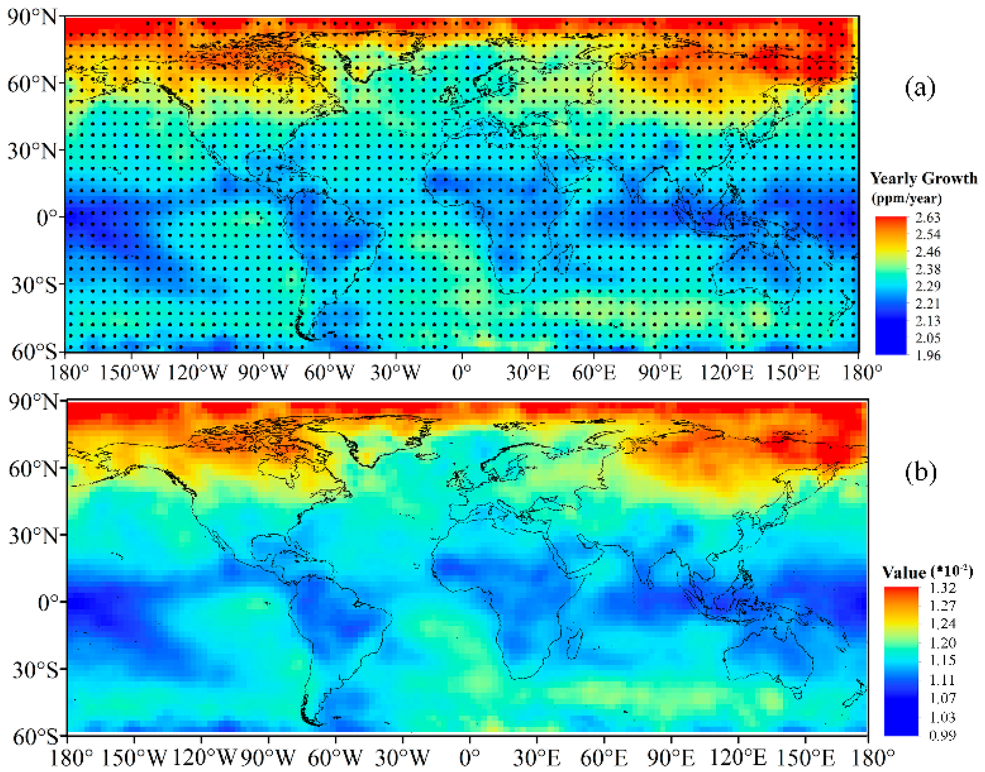
4.2. Analysis of Influencing Factors of Spatial Difference in CO₂ Growth Rate

The regions with higher CO₂ growth rates are located in the high latitudes, while the regions with lower growth rates are located over the oceans at low latitudes (Figure 3). The difference in the spatial distribution of the CO₂ growth rate may be related to the different responses of land at high latitudes and ocean at low latitudes to climate change.

High-latitude permafrost in the Northern Hemisphere is a very large soil carbon pool. With global warming, especially in winter, the permafrost has continued to melt, causing the organic carbon stored in the soil to be released via soil respiration [50,51], resulting in a high annual growth rate of CO₂ in this region, even higher than that in the mid-latitude regions influenced by human activities. The oceans also comprise very large carbon pools. The carbon storage of the oceans is more than 60 times that of the atmosphere (589 PgC) [52]. With the increase in sea water temperature at low latitudes, the utilization of nutrients by surface plants increases, which enhances the bio-carbon pump and produces negative feedback on the increase of atmospheric CO₂ [53,54]. Moreover, the change in water temperature will also affect the solubility of CO₂ in seawater. The solubility of CO₂ decreases with increasing temperature, thus inhibiting the absorption of atmospheric CO₂ by the oceans [55]. Overall, global warming will weaken the ability of oceans to absorb CO₂. However, compared with the high-latitude land region, the ocean at low latitudes remains a carbon sink, which has a negative feedback effect on the CO₂ growth rate. Therefore, the growth rate of CO₂ over the ocean at low latitudes is lower than that over land at high latitudes. The other point that needs to be mentioned is that the spatial difference in the growth rate is very large (maximum: 2.63 ppm/a; minimum: 1.96 ppm/a). The decrease in atmospheric CO₂ detection capability over the ocean, caused by absorption of thermal infrared radiation spectra AIRS used [17,18] by seawater, may reduce the sensitivity of detecting mid-tropospheric CO₂ concentration changes over the ocean, which may increase the spatial difference.

The growth rate from AIRS is always larger than that from ground stations (Table 2). The bias in the retrieval algorithm for inversion of AIRS CO₂ product might contribute to that discrepancy. The AIRS CO₂ product used in this article is retrieved using VPD, which is to iteratively minimize the root mean square (RMS) residual radiance using groups of AIRS channels and obtain the minimum value [31]. The inversion accuracy is affected by many factors, including aerosol, cirrus cloud, temperature, water vapor, and ozone [56]. Due to the uncertainty and complexity of the influencing factors, however, the reasons for the differences in the growth rates between AIRS and land stations are not fully understood and need further investigation.

5. Conclusions

In this study, global mid-tropospheric CO₂ concentrations and the relevant influencing factors were investigated based on an AIRS CO₂ product and relevant auxiliary data. The main conclusions are summarized as follows:

(1) There is a strong correlation between the AIRS-retrieved mid-tropospheric CO₂ product and the data obtained from aircraft observations (R > 0.94). The monthly average difference between the AIRS-retrieved and observed data is less than 0.4 ppm. The AIRS CO₂ product is highly accurate and stable and can be used to capture the seasonal and annual variations in the mid-tropospheric CO₂ concentration.

(2) Global mid-tropospheric CO₂ concentrations display notable spatial heterogeneity. The CO₂ concentrations are higher in the NH than the SH, and higher over land than over the oceans. The high-value areas (30°N–70°N) and low-value areas (20°S–5°N) are distributed in a zonal pattern along the latitudes. The low-mid-tropospheric CO₂ concentration areas are formed as a result of subsidence in the atmosphere, the presence of the Amazon rainforest, and the lack of impact of high-CO₂ emissions. The high-mid-tropospheric CO₂ concentration areas are formed due to high CO₂ emissions and the horizontal and vertical motions of winds.

(3) There is a notable inter-annual increasing trend in mid-tropospheric CO₂ concentrations. In addition, the higher the latitude becomes, the greater the annual average rate of increase.

(4) In various latitude zones around the globe, the higher the latitude, the greater the seasonal fluctuations in mid-tropospheric CO₂ concentrations between consecutive months and seasons. In addition, the fluctuations are more intense in the NH than in the SH. The amplitude of the seasonal variation retrieved from AIRS is consistent with that of CONTRAIL but smaller than that of the surface ground stations, which is related to altitude and coverage.

Although this study analyzed the characteristics of the global spatio-temporal distribution of the mid-tropospheric CO₂ concentration and the most important factors affecting them, the analysis in this study has some level of uncertainty, the magnitude of which is unclear due to the short time scale of the AIRS CO₂ product. This question will be the focus of a future study.

References

1. Dlugokencky, E.; Pieter, T. Trends in Atmospheric Carbon Dioxide. Available online: http://www.esrlnoaa.gov/gmd/ccgg/trends (accessed on 18 May 2018).
2. Houweling, S.; Breon, F.M.; Aben, I.; Rödenbeck, C.; Gloor, M.; Heimann, M.; Ciais, P. Inverse modeling of CO2 sources and sinks using satellite data: A synthetic inter-comparison of measurement techniques and their performance as a function of space and time. Atmos. Chem. Phys. 2004, 4, 523–538. [Google Scholar] [CrossRef]
3. Komhyr, W.D.; Gammon, R.H.; Harris, T.B.; Waterman, L.S.; Conway, T.J.; Taylor, W.R.; Thoning, K.W. Global atmospheric CO2 distribution and variations from 1968–1982 NOAA/GMCC CO2 flask sample data. J. Geophys. Res. 1985, 90, 5567–5596. [Google Scholar] [CrossRef]
4. Bai, W.; Zhang, X.; Zhang, P. Temporal and spatial distribution of tropospheric CO2 over china based on satellite observations. Chin. Sci. Bull. 2010, 55, 3612–3618. [Google Scholar] [CrossRef]
5. Buchwitz, M.; de Beek, R.; Noël, S.; Burrows, J.P.; Bovensmann, H.; Schneising, O.; Khlystova, I.; Bruns, M.; Bremer, H.; Bergamaschi, P.; et al. Atmospheric carbon gases retrieved from SCIAMACHY by WFM-DOAS: Version 0.5 CO and CH4 and impact of calibration improvements on CO2 retrieval. Atmos. Chem. Phys. 2006, 6, 2727–2751. [Google Scholar] [CrossRef]
6. O’Brien, D.M.; Rayner, P.J. Global observations of the carbon budget, 2, CO2 column from differential absorption of reflected sunlight in the 1.61 μm band of CO2. J. Geophys. Res. 2002, 107, 4354. [Google Scholar] [CrossRef]
7. Warneke, T.; Yang, Z.; Olsen, S.; Körner, S.; Notholt, J.; Toon, G.C.; Velazco, V.; Schulz, A.; Schrems, O. Seasonal and latitudinal variations of column averaged volume-mixing ratios of atmospheric CO2. Geophys. Res. Lett. 2005, 32, L03808. [Google Scholar] [CrossRef]
8. Rayner, P.J.; O’Brien, D.M. The utility of remotely sensed CO2 concentration data in surface source inversions. Geophys. Res. Lett. 2001, 28, 175–178. [Google Scholar] [CrossRef]
9. Dai, T.; Shi, G.; Zhang, X.; Xu, N. Influence of HITRAN database updates on retrievals of atmospheric CO2 from near-infrared spectra. Acta Meteorol. Sin. 2012, 26, 629–641. [Google Scholar] [CrossRef]
10. Aumann, H.H.; Chahine, M.T.; Gautier, C.; Goldberg, M.D.; Kalnay, E.; McMillin, L.M.; Revercomb, H.; Rosenkranz, P.W.; Smith, W.L.; Staelin, D.H.; et al. AIRS/AMSU/HSB on the Aqua mission: Design, science objectives, data products, and processing systems. IEEE Trans. Geosci. Remote Sens. 2003, 41, 253–264. [Google Scholar] [CrossRef]
11. Chahine, M.T.; Pagano, T.S.; Aumann, H.H.; Atlas, R.; Barnet, C.; Blaisdell, J.; Chen, L.; Divakarla, M.; Fetzer, E.J.; Goldberg, M.; et al. AIRS: Improving weather forecasting and providing new data on greenhouse gases. Bull. Am. Meteorol. Soc. 2006, 87, 911–926. [Google Scholar] [CrossRef]
12. Crevoisier, C.; Chédin, A.; Matsueda, H.; Machida, T.; Armante, R.; Scott, N.A. First year of upper tropospheric integrated content of CO2 from IASI hyperspectral infrared observations. Atmos. Chem. Phys. 2009, 9, 4797–4810. [Google Scholar] [CrossRef]
13. Bovensmann, H.; Burrows, J.P.; Buchwitz, M.; Frerick, J.; Noel, S.; Rozanov, V.V.; Chance, K.V.; Goede, A.P.H. SCIAMACHY: Mission objectives and measurement modes. J. Atmos. Sci. 1999, 56, 127–150. [Google Scholar] [CrossRef]
14. Noël, S.; Bovensmann, H.; Burrows, J.P.; Frerick, J.; Chance, K.V.; Goede, A.H.P. Global atmospheric monitoring with SCIAMACHY. Phys. Chem. Earth Part C 1999, 24, 427–434. [Google Scholar] [CrossRef]
15. Yokota, T.; Yoshida, Y.; Eguchi, N.; Ota, Y.; Tanaka, T.; Watanabe, H.; Maksyutov, S. Global concentrations of CO2 and CH4 retrieved from GOSAT: First preliminary results. Sola 2009, 5, 160–163. [Google Scholar] [CrossRef]
16. Yoshida, Y.; Ota, Y.; Eguchi, N.; Kikuchi, N.; Nobuta, K.; Tran, H.; Morino, I.; Yokota, T. Retrieval algorithm for CO2 and CH4 column abundances from short-wavelength infrared spectral observations by the Greenhouse gases observing satellite. Atmos. Meas. Tech. 2011, 4, 717–734. [Google Scholar] [CrossRef]
17. Barkley, M.P.; Monks, P.S.; Engelen, R.J. Comparison of SCIAMACHY and AIRS CO2 measurements over North America during the summer and autumn of 2003. Geophys. Res. Lett. 2006, 33. [Google Scholar] [CrossRef]
18. Zhang, L.; Jiang, H.; Zhang, X. Comparison analysis of the global carbon dioxide concentration column derived from SCIAMACHY, AIRS, and GOSAT with surface station measurements. Int. J. Remote Sens. 2015, 36, 1406–1423. [Google Scholar] [CrossRef]
19. Crevoisier, C.; Heilliette, S.; Chédin, A.; Serrar, S.; Armante, R.; Scott, N.A. Midtropospheric CO2 concentration retrieval from AIRS observations in the tropics. Geophys. Res. Lett. 2004, 31. [Google Scholar] [CrossRef]
20. Maddy, E.S.; Barnet, C.D.; Goldberg, M.; Sweeney, C.; Liu, X. CO2 retrievals from the Atmospheric Infrared Sounder: Methodology and validation. J. Geophys. Res. 2008, 113, D11301. [Google Scholar] [CrossRef]
21. Zhang, L.; Zhang, X.; Jiang, H. Accuracy comparisons of AIRS, SCIAMACHY and GOSAT with ground-based data based on global CO2 concentration. In Proceedings of the 2013 21st International Conference on Geoinformatics, Kaifeng, China, 20–22 June 2013; pp. 1–5. [Google Scholar]
22. Zhang, L.L.; Yue, T.X.; Wilson, J.P.; Zhao, N.; Zhao, Y.P.; Du, Z.P.; Liu, Y. A comparison of satellite observations with the XCO2 surface obtained by fusing TCCON measurements and GEOS-Chem model outputs. Sci. Total Environ. 2017, 601, 1575–1590. [Google Scholar] [CrossRef]
23. Jiang, X.; Crisp, D.; Olsen, E.T.; Kulawik, S.S.; Miller, C.E.; Pagano, T.S.; Liang, M.; Yung, Y.L. CO2 annual and semiannual cycles from multiple satellite retrievals and models. Earth Space Sci. 2016, 3, 78–87. [Google Scholar] [CrossRef]
24. Jing, Y.; Shi, J.; Wang, T.; Sussmann, R. Mapping Global Atmospheric CO2 Concentration at High Spatiotemporal Resolution. Atmos 2014, 5, 870–888. [Google Scholar] [CrossRef]
25. Pagano, T.S.; Olsen, E.T.; Chahine, M.T.; Ruzmaikin, A.; Nguyen, H.; Jiang, X. Monthly representations of mid-tropospheric carbon dioxide from the atmospheric infrared sounder. In Proceedings of the Imaging Spectrometry XVI, San Diego, CA, USA, 6 September 2011. [Google Scholar]
26. Pagano, T.S.; Olsen, E.T.; Hai, N.; Ruzmaikin, A.; Jiang, X.; Perkins, L. Global variability of midtropospheric carbon dioxide as measured by the Atmospheric Infrared Sounder. J. Appl. Remote Sens. 2014, 8, 084984. [Google Scholar] [CrossRef]
27. Kumar, K.R.; Revadekar, J.V.; Tiwari, Y.K. AIRS retrieved CO2 and its association with climatic parameters over India during 2004-2011. Sci. Total Environ. 2014, 476, 79–89. [Google Scholar] [CrossRef]
28. Tiwari, Y.K.; Revadekar, J.V.; Kumar, K.R. Variations in atmospheric Carbon Dioxide and its association with rainfall and vegetation over India. Atmos. Environ. 2013, 68, 45–51. [Google Scholar] [CrossRef]
29. Tiwari, Y.K.; Revadekar, J.V.; Kumar, K.R. Anomalous features of mid-tropospheric CO2 during Indian summer monsoon drought years. Atmos. Environ. 2014, 99, 94–103. [Google Scholar] [CrossRef]
30. Chahine, M.T.; Chen, L.; Dimotakis, P.; Jiang, X.; Li, Q.; Olsen, E.T.; Pagano, T.; Randerson, J.; Yung, Y.L. Satellite remote sounding of mid-tropospheric CO2. Geophys. Res. Lett. 2008, 35, L17807. [Google Scholar] [CrossRef]
31. Chahine, M.; Barnet, C.; Olsen, E.T.; Chen, L.; Maddy, E. On the determination of atmospheric minor gases by the method of vanishing partial derivatives with application to CO2. Geophys. Res. Lett. 2005, 32, L22803. [Google Scholar] [CrossRef]
32. Engelen, R.J.; McNally, A.P. Estimating atmospheric CO2 from advanced infrared satellite radiances within an operational four-dimensional variational (4D-Var) data assimilation system: Results and validation. J. Geophys. Res. 2005, 110, D18305. [Google Scholar] [CrossRef]
33. Kumar, K.R.; Tiwari, Y.K.; Revadekar, J.V.; Vellore, R.; Guha, T. Impact of ENSO on variability of AIRS retrieved CO2 over India. Atmos. Environ. 2016, 142, 83–92. [Google Scholar] [CrossRef]
34. Olsen, E.T.; Licata, S.J. AIRS Version 5 Release Tropospheric CO2 Products. Available online: https://docserver.gesdisc.eosdis.nasa.gov/repository/Mission/AIRS/3.3_ScienceDataProductDocumentation/3.3.4_ProductGenerationAlgorithms/AIRS-V5-Tropospheric-CO2-Products.pdf (accessed on 6 Septemper 2018).
35. Machida, T.; Matsueda, H.; Sawa, Y.; Nakagawa, Y.; Hirotani, K.; Kondo, N.; Goto, K.; Nakazawa, T.; Ishikawa, K.; Ogawa, T. Worldwide measurements of atmospheric CO2 and other trace gas species using commercial airlines. J. Atmos. Ocean. Technol. 2008, 25, 1744–1754. [Google Scholar] [CrossRef]
36. Umezawa, T.; Matsueda, H.; Sawa, Y.; Niwa, Y.; Machida, T.; Zhou, L. Seasonal evaluation of tropospheric CO2 over the Asia-Pacific region observed by the CONTRAIL commercial airliner measurements. Atmos. Chem. Phys. Discuss. 2018, 2018, 1–28. [Google Scholar] [CrossRef]
37. Janssens-Maenhout, G.; Crippa, M.; Guizzardi, D.; Muntean, M.; Schaaf, E.; Dentener, F.; Bergamaschi, P.; Pagliari, V.; Olivier, J.G.J.; Peters, J.A.H.W.; et al. EDGAR v4.3.2 Global Atlas of the three major Greenhouse Gas Emissions for the period 1970–2012. Earth Syst. Sci. Data Discuss. 2017, 2017, 1–55. [Google Scholar] [CrossRef]
38. Kalnay, E.; Kanamitsu, M.; Kistler, R.; Collins, W.; Deaven, D.; Gandin, L.; Iredell, M.; Saha, S.; White, G.; Woollen, J.; et al. The NCEP/NCAR 40-Year Reanalysis Project. Bull. Am. Meteorol. Soc. 1996, 77, 437–472. [Google Scholar] [CrossRef]
39. Hannachi, A.; Jolliffe, I.T.; Stephenson, D.B. Empirical orthogonal functions and related techniques in atmospheric science: A review. Int. J. Climatol. 2007, 27, 1119–1152. [Google Scholar] [CrossRef] [Green Version]
40. Weare, B.C.; Nasstrom, J.S. Examples of extended empirical orthogonal function analyses. Mon. Weather Rev. 1982, 110, 481–485. [Google Scholar] [CrossRef]
41. North, G.R.; Bell, T.L.; Cahalan, R.F.; Moeng, F.J. Sampling errors in the estimation of empirical orthogonal functions. Mon. Weather Rev. 1982, 110, 699–706. [Google Scholar] [CrossRef]
42. Dettinger, M.D.; Ghil, M. Seasonal and interannual variations of atmospheric CO2 and climate. Tellus B Chem. Phys. Meteorol. 1998, 50, 1–24. [Google Scholar] [CrossRef]
43. Cochran, F.; Brunsell, N. Temporal scales of tropospheric CO2, precipitation, and ecosystem responses in the central Great Plains. Remote Sens. Environ. 2012, 127, 316–328. [Google Scholar] [CrossRef]
44. Cao, L.; Chen, X.; Zhang, C.; Kurban, A.; Yuan, X.; Pan, T.; de Maeyer, P. The Temporal and Spatial Distributions of the Near-Surface CO2 Concentrations in Central Asia and Analysis of Their Controlling Factors. Atmos 2017, 8, 85. [Google Scholar] [CrossRef]
45. Krishnamurti, T.N. Tropical East-West Circulations During the Northern Summer. J. Atmos. Sci. 1971, 28, 1342–1347. [Google Scholar] [CrossRef] [Green Version]
46. Mancuso, R.L. A Numerical Procedure for Computing Fields of Stream Function and Velocity Potential. J. Appl. Meteorol. 1967, 6, 994–1001. [Google Scholar] [CrossRef] [Green Version]
47. Wang, C. Atlantic Climate Variability and Its Associated Atmospheric Circulation Cells. J. Clim. 2002, 15, 1516–1536. [Google Scholar] [CrossRef]
48. Wang, C. Atmospheric Circulation Cells Associated with the El Niño–Southern Oscillation. J. Clim. 2002, 15, 399–419. [Google Scholar] [CrossRef]
49. Brienen, R.J.W.; Phillips, O.L.; Feldpausch, T.R.; Gloor, E.; Baker, T.R.; Lloyd, J.; Lopez-Gonzalez, G.; Monteagudo-Mendoza, A.; Malhi, Y.; Lewis, S.L.; et al. Long-term decline of the amazon carbon sink. Nature 2015, 519, 344. [Google Scholar] [CrossRef] [PubMed]
50. Schaefer, K.; Zhang, T.; Bruhwiler, L.; Barrett, A.P. Amount and timing of permafrost carbon release in response to climate warming. Tellus B Chem. Phys. Meteorol. 2011, 63, 168–180. [Google Scholar] [CrossRef]
51. Zimov, S.; Davidov, S.; Voropaev, Y.V.; Prosiannikov, S.; Semiletov, I.; Chapin, M.; Chapin, F. Siberian CO2 efflux in winter as a CO2 source and cause of seasonality in atmospheric CO2. Clim. Chang. 1996, 33, 111–120. [Google Scholar] [CrossRef]
52. Ciais, P.; Sabine, C.; Bala, G.; Bopp, L.; Brovkin, V.; Canadell, J.; Chhabra, A.; DeFries, R.; Galloway, J.; Heimann, M.; et al. Carbon and other biogeochemical cycles. In Climate Change 2013: The Physical Science Basis. Contribution of Working Group I to the Fifth Assessment Report of the Intergovernmental Panel on Climate Change; Cambridge University Press: Cambridge, UK; New York, NY, USA, 2014; pp. 465–570. ISBN 9781107415324. [Google Scholar]
53. Ito, T.; Follows, M. Preformed phosphate, soft tissue pump and atmospheric CO2. J. Mar. Res. 2005, 63, 813–839. [Google Scholar] [CrossRef]
54. Sarmiento, J.L.; Slater, R.; Barber, R.; Bopp, L.; Doney, S.C.; Hirst, A.; Kleypas, J.; Matear, R.; Mikolajewicz, U.; Monfray, P.; et al. Response of ocean ecosystems to climate warming. Glob. Biogeochem. Cycles 2004, 18, GB3003. [Google Scholar] [CrossRef]
55. Riebesell, U.; Körtzinger, A.; Oschlies, A. Sensitivities of marine carbon fluxes to ocean change. Proc. Natl. Acad. Sci. USA 2009, 106, 20602–20609. [Google Scholar] [CrossRef] [Green Version]
56. Olsen, E.T.; Chahine, M.T.; Chen, L.L.; Pagano, T.S. Retrieval of mid-tropospheric CO2 directly from AIRS measurements. In Algorithms and Technologies for Multispectral, Hyperspectral, and Ultraspectral Imagery XIV; International Society for Optics and Photonics: Bellingham, WA, USA, 2008; p. 696613. [Google Scholar]
Figure 1. Comparison of the atmospheric infrared sounder (AIRS) data with aircraft observations in six areas from 2003 to 2011. (a) Comprehensive observation network for trace gases by airliner (CONTRAIL) a area; (b) CONTRAIL b area; (c) CONTRAIL c area; (d) CONTRAIL d area; (e) CONTRAIL e area; (f) CONTRAIL f area.
Remotesensing 11 00094 g001
Figure 2. Annual average global distribution of the mid-troposphere CO2 concentration from 2003 to 2011.
Remotesensing 11 00094 g002
Figure 3. The spatial variation pattern of the global annual mean mid-tropospheric CO2 concentration from 2003 to 2011 based on different methods. (a) OLS regression; (b) empirical orthogonal function (EOF). Pixels with black point are statistically significant at p < 0.05.
Remotesensing 11 00094 g003
Figure 4. Hovmöller diagram of the AIRS monthly mid-tropospheric CO2 concentrations by latitude (a) and longitude (b).
Remotesensing 11 00094 g004
Figure 5. Temporal variation of the mid-tropospheric CO2 concentration in different regions around the world based on the AIRS data from 2003 to 2011. (a) Monthly mid-tropospheric CO2 concentration in the Northern Hemisphere (NH); (b) Monthly mid-tropospheric CO2 concentration in the Southern Hemisphere (SH); (c) Seasonal mid-tropospheric CO2 concentration in the NH; (d) Seasonal mid-tropospheric CO2 concentration in the SH; (e) Monthly variability in the detrended mid-tropospheric CO2 concentration; (f) Seasonal variability of the detrended mid-tropospheric CO2 concentration.
Remotesensing 11 00094 g005
Figure 6. Comparison of seasonal cycles of CO2 concentration retrieved from AIRS with that derived from the World Data Center for Greenhouse Gases (WDCGG) ground-based measurements from 2003 to 2011. (a) Anmyeon-do; (b) Assekrem; (c) Mt. Dodaira; (d) Niwot Ridge; (e) Izaña; (f) Kisai; (g) Mauna Loa; (h) Yonagunijima.
Remotesensing 11 00094 g006
Figure 7. Comparison of seasonal cycles of CO2 concentration retrieved from AIRS with that measured by CONTRAIL from 2003 to 2011. (a) CONTRAIL a area; (b) CONTRAIL b area; (c) CONTRAIL c area; (d) CONTRAIL d area; (e) CONTRAIL e area; (f) CONTRAIL f area.
Remotesensing 11 00094 g007
Figure 8. The multi-year average (2003–2011) climatologies of tropospheric circulation patterns. (a) 200-mb velocity potential (106 m2 s−1) and wind divergence (m s−1); (b) 200-mb stream function (106 m2 s−1) and wind vorticity (m s−1); (c) 500-mb vertical velocity (Pa s−1); (d) 500-mb stream function (106 m2 s−1) and wind vorticity (m s−1); (e) 1000-mb velocity potential (106 m2 s−1) and wind divergence (m s−1); (f) 500-mb stream function (106 m2 s−1) and wind vorticity (m s−1); (g) zonal-vertical circulation cross section in the west calculated by averaging the wind divergence and the vertical velocity between 30°N and 70°N; (h) zonal-vertical circulation cross section in the west calculated by averaging the wind divergence and the vertical velocity between 20°S and 5°N. The vertical velocity is taken to be the negative of the pressure vertical velocity in the re-analysis.
Remotesensing 11 00094 g008
Figure 9. Global annual average distribution of CO2 emissions between 2003 and 2011.
Remotesensing 11 00094 g009