Article

SAR Interferometry for Sinkhole Early Warning and Susceptibility Assessment along the Dead Sea, Israel

1
Geological Survey of Israel, Jerusalem 95501, Israel
2
Dead-Sea & Arava Science Center, Massada 86910, Israel
3
School of Environmental and Earth Sciences, Tel-Aviv University, Tel-Aviv 6997801, Israel
4
Istituto Nazionale di Geofisica e Vulcanologia, 00143 Rome, Italy
*
Author to whom correspondence should be addressed.
Remote Sens. 2019, 11(1), 89; https://doi.org/10.3390/rs11010089
Submission received: 28 November 2018 / Revised: 19 December 2018 / Accepted: 2 January 2019 / Published: 7 January 2019
(This article belongs to the Special Issue Remote Sensing of Land Subsidence)

Abstract

:
During the past three decades, the Dead Sea (DS) water level has dropped at an average rate of ~1 m/year, resulting in the formation of thousands of sinkholes along its coastline that severely affect the economy and infrastructure of the region. The sinkholes are associated with gradual land subsidence, preceding their collapse by periods ranging from a few days to about five years. We present the results of over six years of systematic high temporal and spatial resolution interferometric synthetic aperture radar (InSAR) observations, incorporated with and refined by detailed Light Detection and Ranging (LiDAR) measurements. The combined data enable the utilization of interferometric pairs with a wide range of spatial baselines to detect minute precursory subsidence before the catastrophic collapse of the sinkholes and to map zones susceptible to future sinkhole formation. We present here four case studies that illustrate the timelines and effectiveness of our methodology as well as its limitations and complementary methodologies used for sinkhole monitoring and hazard assessment. Today, InSAR-derived subsidence maps have become fundamental for sinkhole early warning and mitigation along the DS coast in Israel and are incorporated in all sinkhole potential maps which are mandatory for the planning and licensing of new infrastructure.

1. Introduction

Collapse sinkholes occur in a large number of geological environments around the globe e.g., [1,2,3]. They generally form by the dissolution of subsurface soluble rocks, creating cavities that collapse when insufficiently supported [4,5,6]. Sinkholes are commonly associated with gradual, dissolution-induced land subsidence, which occurs before, during, and after the surface collapse of the sinkhole [7,8,9,10,11]. The duration and magnitude of the precursory subsidence were determined by InSAR measurements, LiDAR elevation models, and field observations, and were found to correlate with the mechanical properties of the sediments [12].
Over ~6000 collapse sinkholes (Figure 1) have been mapped along the DS shores since they were first discovered in the 1980s [13], with a persistently increasing formation rate that reached ~400 sinkholes in 2017 and peaked with ~700 new sinkholes in 2015 [14] Figure 2. This type of natural hazard affects the local agriculture, industry, tourism, infrastructure, and daily life in the region. The DS sinkholes form as a result of the dissolution of a ~10,000 year old, 5–20 m thick salt (halite) layer buried at depths between 5 m and 65 m along the DS shores [15]. The DS water level currently drops at a rate of more than 1 m/yr (Figure 2) due to the negative balance between influx (precipitation and drainage) and outflux (evaporation and industrial consumption), resulting in the exposure of the salt layer to unsaturated water with respect to halite, dissolution, and the formation of cavities that eventually collapse as sinkholes [16].
The sinkholes commonly form along lineaments that follow concealed faults [18], or the margins of the subsurface salt layer [19]. The sinkholes’ diameters range from less than a meter to ~40 m. They are clustered in ~50 sites and are surrounded in places by gradually subsiding zones ranging in length and width from less than 100 m to more than 1000 m, which were first detected by low resolution InSAR measurements [20]. The sinkholes appear in two main sedimentary environments of the DS coast [21]: mudflats consisting of fine-grained lacustrine sediments, and alluvial fans composed of coarse-grained fluvial sediments. The depth to the top of the salt layer is between 25 m and 65 m in the alluvial fans and usually less than 20 m at the mudflats [15,22]. The sediments of these two environments differ in their mechanical properties: the alluvial fan sediments deform mostly as brittle material attested by the steep walls of the sinkholes and stream channels, whereas the fine-grained sediments in the mudflats deform in a more viscous manner [12,23]. The differences in salt depth and sediment rheology affect sinkhole collapse in two ways. First, sinkholes in the alluvial fans tend to be deeper (the deepest is ~27 m) and narrower than those in the mudflats. Second, field and InSAR observations, and mechanical models [12,23,24,25] indicate that the thick and stiff overburden in the alluvial fans impedes final collapse into the awaiting cavity in the salt layer. This may cause a delay of several years between sinkhole formation in an alluvial fan and an adjacent mudflat [25]. This difference between the two environments also causes a significant difference in the duration of precursory subsidence before the collapse of individual sinkholes [12].
Various geophysical methods have been previously used for monitoring and detecting sinkholes along the DS before their collapse, with varying degrees of success [25,26,27,28]. However, all of these methods are limited to specific sites and require on-ground equipment and operating personnel, either continuously or periodically. Here, we present the use of InSAR for sinkhole early warning, susceptibility assessment, and risk reduction along the DS. First, we present a technical overview of the sinkhole early warning monitoring system. Then, we show four case studies where InSAR has been successfully utilized for the above-mentioned purposes, and finally, we discuss the system’s limitation, application, and outlook.

2. Materials and Methods

2.1. InSAR Data and Processing

We used the Italian Space Agency (ASI) COSMO-SkyMed (CSK) X-band (wavelength 3.1 cm) radar images (HIMAGE mode) acquired every 16 days from ascending and descending orbits. To geocode and remove the topographic phase components in the InSAR measurements, we first used a global digital elevation model (GDEM) of the one arc-second Advanced Spaceborne Thermal Emission and Reflection Radiometer (ASTER) satellite, which is considered to have a vertical accuracy of 17 m at the 95% confidence level [29]. The perpendicular baseline of the interferograms ranges from 12 m to ~1500 m with an average of ~500 m. At a given platform altitude of ~620 km and a typical look angle of 41°, this would result in an altitude of ambiguity [30] of ~12 m in many of the interferograms, comparable to the GDEM error. To minimize the DEM errors in the sinkhole areas, we incorporated an airborne LiDAR digital surface model (DSM) of the DS shores with a spatial resolution of 0.5 m, an absolute elevation error of less than 0.35 m, and a spatial uncertainty of less than 1 m [31] into the ASTER GDEM. One limitation of the LiDAR DSM is that the elevation data include surface objects (e.g., power lines and vegetation), and their sharp relief may result in data gaps due to shadowed or overlaid areas where no interferometric phase can be calculated. LiDAR measurements have been updated each year since 2011 and the composite ASTER-LiDAR DEM model is updated when new data are available. The GDEM and the LiDAR data are resampled to match the CSK spatial resolution of 3 × 3 m and the GDEM data are populated by the LiDAR data using the GDAL/OGR library [32]. The composite ASTER-LiDAR DEM eliminates most of the topographic artifacts and dramatically increases the spatial resolution within the areas covered by LiDAR (Figure 3), thus enabling deformation monitoring at the spatial scale of individual sinkholes and the identification of small footprint (down to 10 × 10 m) sinkhole-related subsidence. It also enables the exploitation of most of the SAR dataset including scenes with perpendicular baselines >1000 m.
Our current dataset consisted of 82 ascending (south to north orbital pass) and 110 descending (north to south) scenes acquired between 14 December, 2011 and 9 May, 2018. More than 180 individual interferograms were generated using the Gamma software [33], spanning periods between 1 and 100 days. The interferograms were generated at full resolution (pixel size of ~3 × 3 m) and filtered using an adaptive filter function based on the local fringe spectrum [34], with a window size of 16 × 16 pixels. Given the small size of the sinkholes (several meters), orbit re-estimation or scene-wide gradient correction was not required as this procedure corrects for distortions of longer spatial wavelengths. The satellite to ground line-of-sight (LOS) displacements (incidence angles of 29°–56° from vertical, right-looking) represent the resultant combination of vertical and horizontal movements for each pixel.

2.2. Monitoring Procedure

A semi-automatic processing system has been developed at the Geological Survey of Israel (GSI) for InSAR monitoring of sinkhole precursors and for sinkhole early warning along the DS shores in Israel. The monitoring and alerting procedure is as follows (Figure 4 and Figure 5):
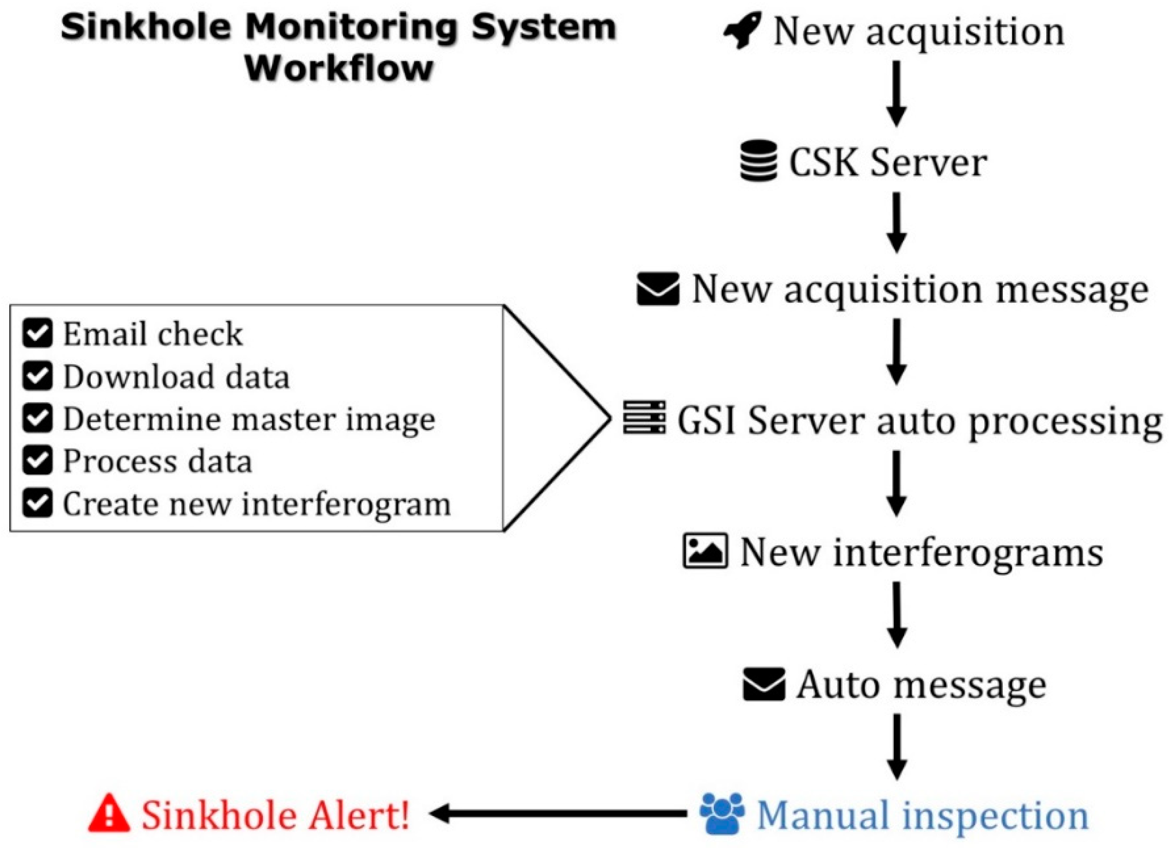
  • Upon the acquisition of a new SAR image, an email message is sent by ASI to GSI, typically within less than 12 h from the acquisition.
  • The system scans a dedicated mail account for such messages and as soon as one is detected, the new data are downloaded within ~3 additional hours.
  • The data are processed into geocoded interferograms of the entire DS region (see below) within ~1 h.
  • All interferograms are inspected and compared with previous interferograms and other independent information (e.g., LiDAR-based sinkhole maps, field reports, etc.) to identify new subsiding areas >10 m from any mapped sinkhole. This procedure is completed within two days.
  • Upon detection of a new subsiding area, it is flagged, the alert level is set from green (no alert) to yellow (watch alert), and early warning alerts are sent to the relevant authorities and stakeholders.
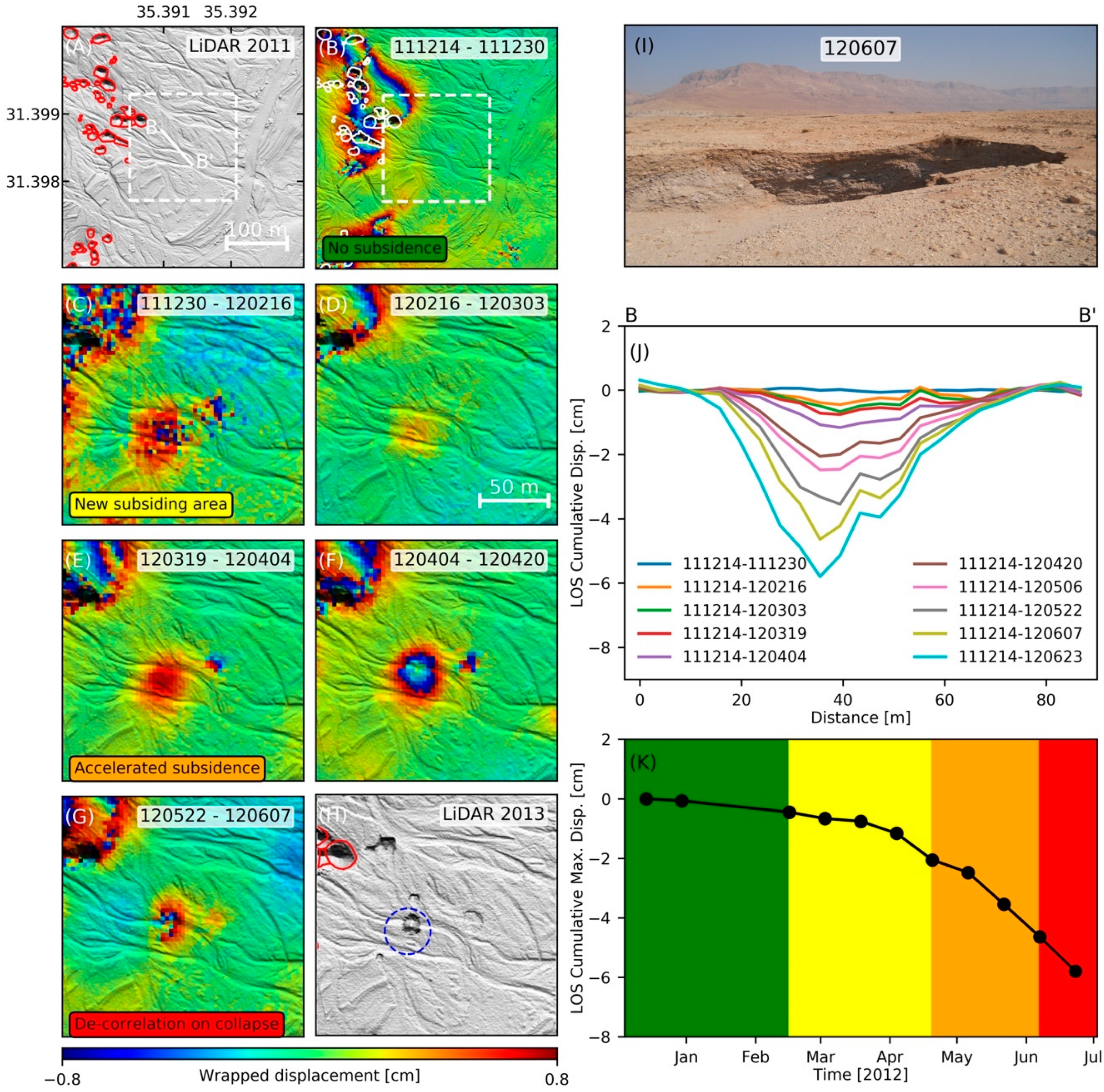
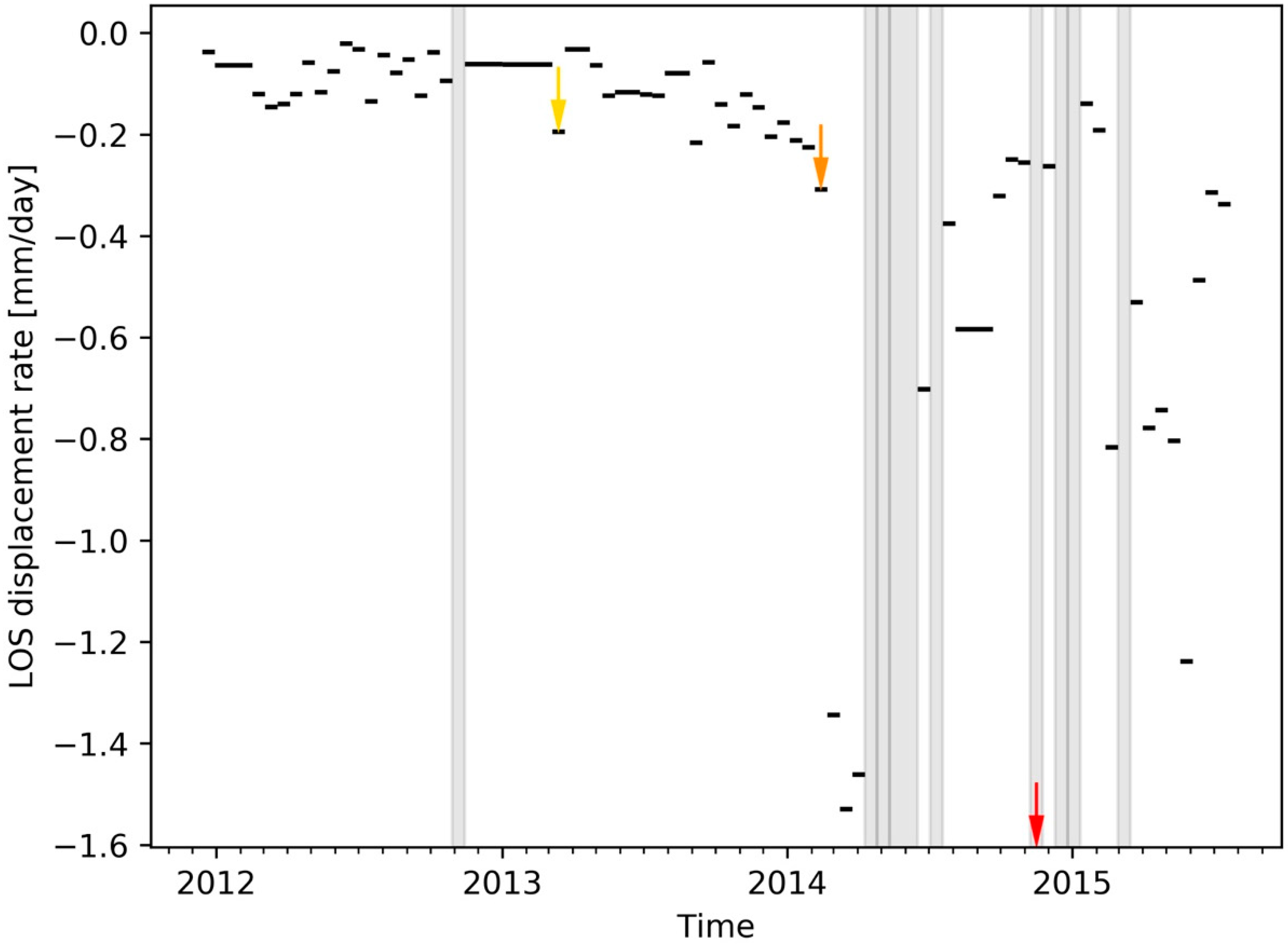
  • The time series of the unwrapped individual interferograms of these areas is progressively analyzed to update the alert level (Figure 5). Upon identification of accelerated subsidence at a site (which is not always visible), the alert level is raised to orange (urgent action alert). Identification of de-correlation in all or part of a subsiding area (excluding cases where de-correlation is clearly due to known weather conditions or extremely large perpendicular baselines) is considered as newly formed sinkholes and the alert level is raised to red (open pits).
We currently monitor displacements along the DS shore at 16-day intervals. The processing system allows us to produce an early warning for a new sinkhole in less than 48 h after data acquisition as long as the interferometric pair carries a coherent signal. In order to identify a sinkhole by coherence loss, we require at least 2 × 2 incoherent pixels. With the current pixel size, this would translate to an area of 6 × 6 m, therefore the minimal collapse size detection limit would be of that order. The validation of new sinkhole collapses is carried out by field observations, drone photos, aerial photos, and LiDAR measurements.

3. Application of InSAR Measurements for Sinkhole Hazard Mitigation

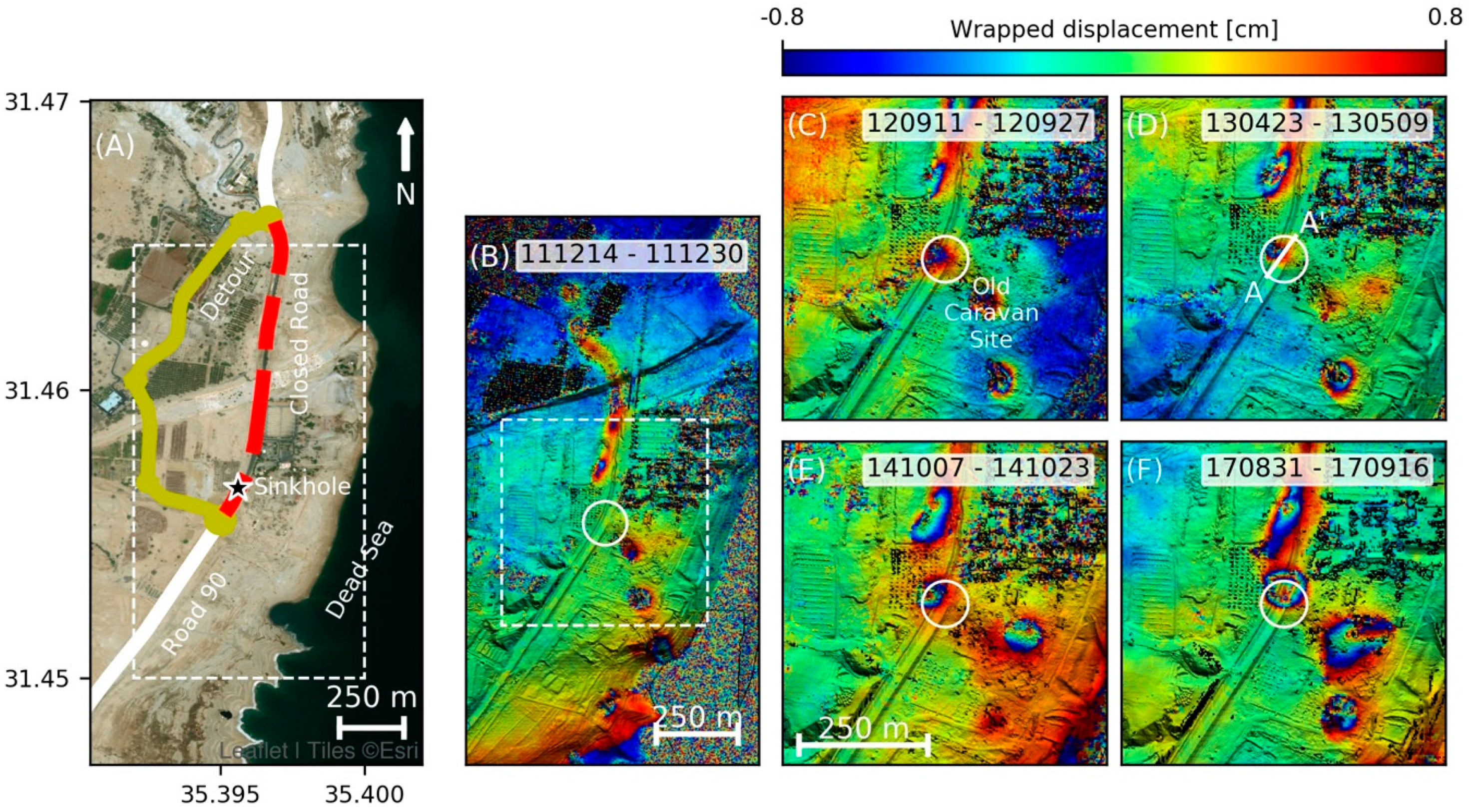
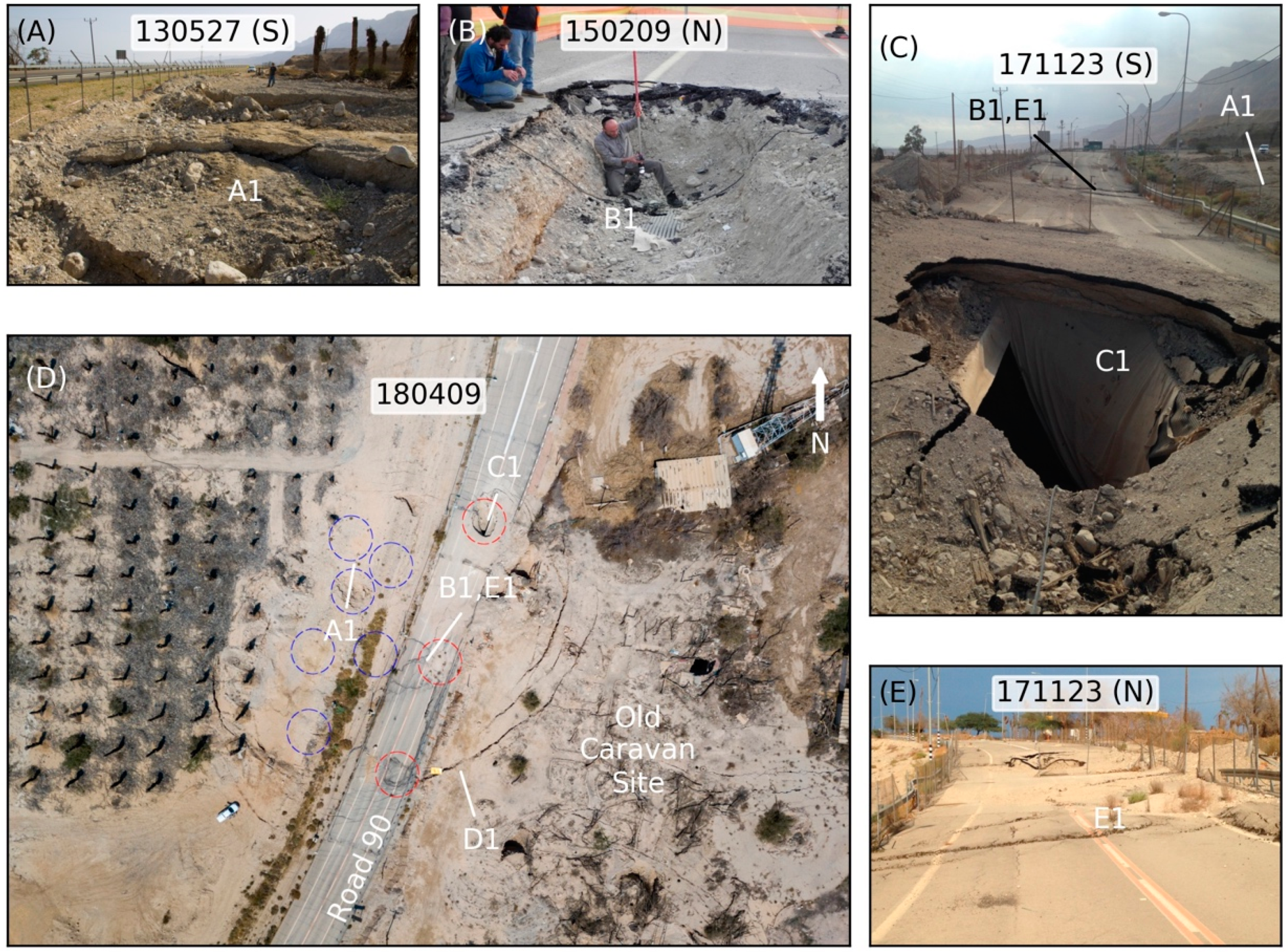
3.1. Early Detection of Sinkhole Precursory Subsidence, Road 90

3.1.1. Site and Hazard

Road 90 is the main eastern route that connects the southern desert districts of Israel to the more populated and humid northern districts. This is also the only road that connects the DS area to the rest of the country. The road has been severely threatened by sinkholes in the area of En Gedi (Figure 1 and Figure 6A). An elongated cluster of sinkholes and their associated gradual subsidence crosses Road 90 obliquely from NNW to SSE (Figure 6B). The sinkhole site has been active since the mid 1990s [21]. To protect the road from sinkhole collapse, geosynthetic sheets were placed in 2002 ~1 m under its surface at its intersection with the sinkhole lineament. Between 2002 and 2012, subsidence and sinkhole collapses continued along the lineament, while the road at its intersection with the subsidence lineament showed no subsidence, most likely due to its reinforcement.

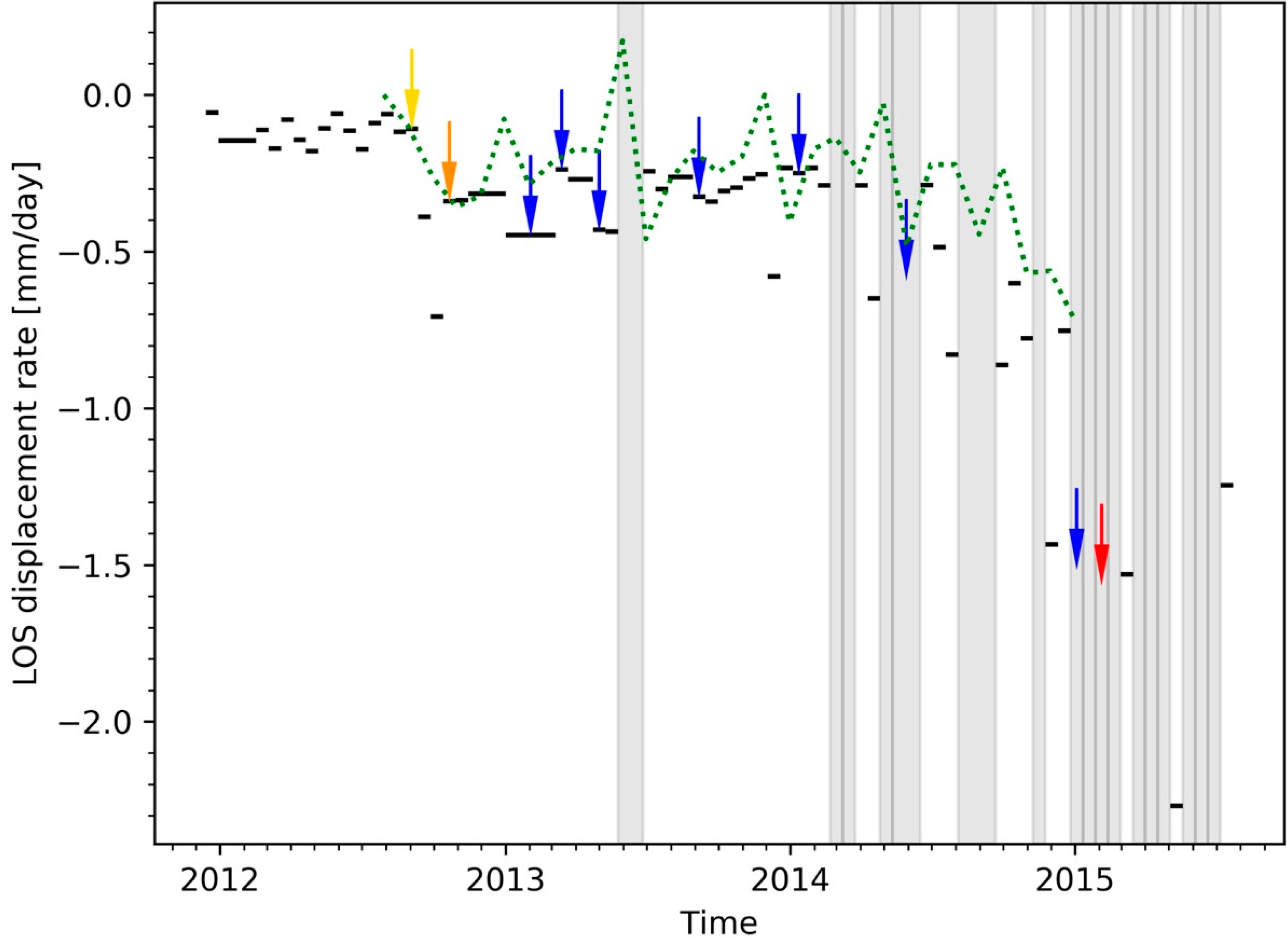
3.1.2. InSAR Monitoring and Early Warning

During the first nine months of 2012, our InSAR monitoring showed very minor subsidence of <0.2 mm/day along the road at its intersection with the sinkhole lineament (Figure 6B and Figure 7). Subsidence rates increased to values of ~0.4 mm/day after mid-September 2012 (Figure 6C and Figure 7), and on October 14 an alert was sent to the National Transport Infrastructure Company (NTIC). Subsidence continued through 2013 and 2014 along with the repeated formation and gravel filling of new sinkholes at the margins of the road, where no reinforcement existed (Figure 7 and Figure 8A). InSAR measurements showed continued and accelerated subsidence in 2013 and 2014 (Figure 6D,E and Figure 7), while the NTIC began planning a bypass that encircled the estimated western margins of the subsurface salt layer. By late 2014, cracks and small depressions appeared on the road as the bypass was almost complete. Road 90 was closed to traffic on 26 January, 2015. On 1 February, 2015 the road was dredged, exposing the geosynthetic sheet, and a 5 m wide, 9 m deep sinkhole was discovered under the road at the center of the subsiding area, directly below the sheet (Figure 8B,D). At that stage, the traffic was already diverted to the new bypass (marked in yellow in Figure 6A). The road surface continued subsiding for almost three more years until in early November 2017, the sheet-supported roof collapsed at the margins of the subsiding area, about 20 m north of the sinkhole that was revealed in February 2015 (Figure 8C,D). The early warning of more than two years provided ample time for the NTIC to construct an alternative route, using InSAR maps of the subsiding areas as guidelines. The abandoned road continues to subside at a rate of ~2 mm/day (Figure 6F), new collapses appear along the road and at the margins of the subsiding area (Figure 8D), while its center shows compressional deformation (Figure 8E), in accordance with elastic model predictions [35].

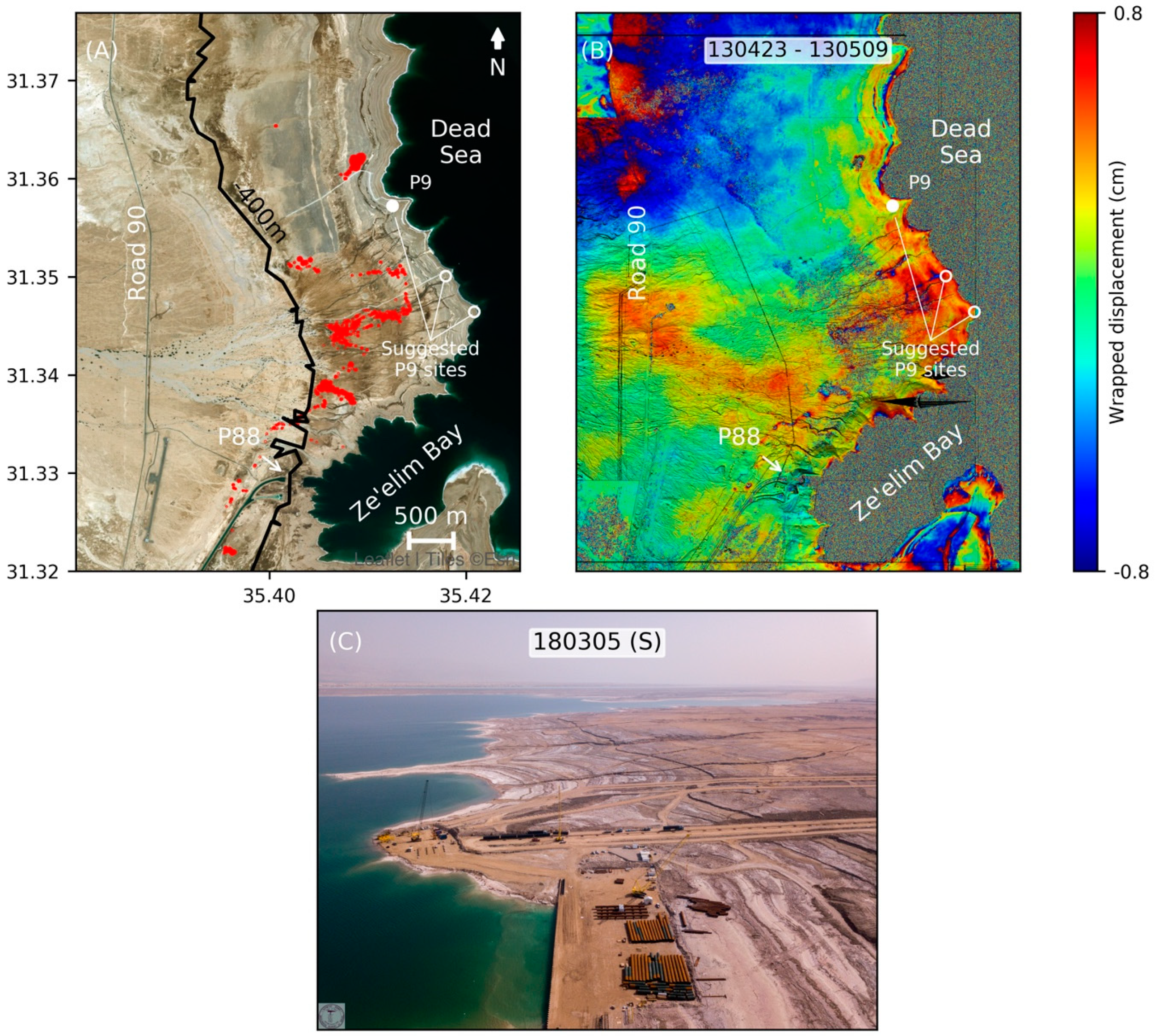
3.2. Infrastructure Risk Reduction, Ze’elim Fan

3.2.1. Site and Hazard

The Ze’elim alluvial fan is the outlet of one of the largest drainage basins along the western coast of the DS, occupying an area of about 250 km2 (Figure 9A). It is dominated by gravel west of the elevation contour of −400 m (black contour line in Figure 9A) and by mudflats east of that contour. The DS mineral industry, Dead Sea Works (DSW), operates pumping stations to convey the DS water from the northern basin to the evaporation pans at the southern basin. The current pumping station (P88, Figure 9A) is about to terminate its lifetime in ~2020, due to the desiccation of the southern Ze’elim Bay, requiring a new pumping station in a location with a deeper sea floor. The precise location of the new pumping station (P9) has been under debate for several years and three alternative sites have been proposed (Figure 9A). The various factors taken into consideration for the new site included the size of the area taken from the public, flash-flood risk, and the current and future sinkhole risk at the proposed new site.

3.2.2. InSAR Measurements for Hazard Evaluation

Continuous InSAR monitoring of the entire Ze’elim fan (Figure 9B) enabled the clear identification of active subsidence in the areas surrounding the southern two sites and their outgoing pipelines. The GSI thus recommended choosing the northern alternative, which was away from active subsidence. This alternative was finally chosen and is currently under construction (Figure 9C). We continue to monitor the ongoing site construction work and subsidence along the entire track of the water conduit from the pumping station to the evaporation ponds, alerting for new potential sinkholes that may put infrastructure or DSW workers at risk.

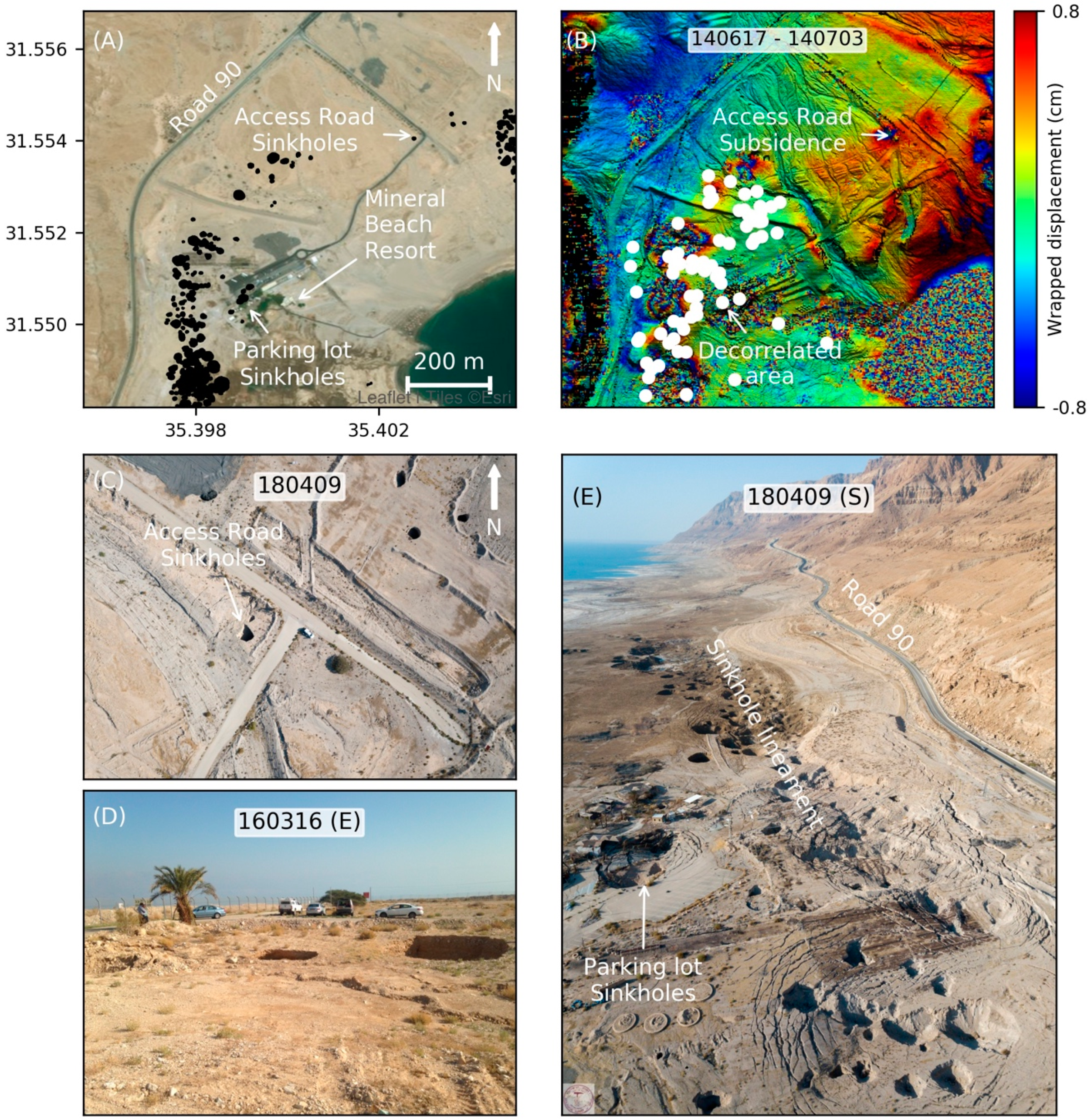
3.3. InSAR and Complementary Monitoring Methods, Mineral Beach

3.3.1. Site and Hazard

Mineral Beach Resort, a tourist attraction and a major income source for the local population, hosted hundreds of visitors daily, and is located upon an alluvial fan east of Road 90 (Figure 10A). A sinkhole lineament separates the resort from Road 90 (Figure 10). It has been studied extensively by boreholes, groundwater geochemistry, seismic refraction and reflection surveys, and other geophysical methods [15,24,25,26,36]. The first sinkholes in this region were formed in the mudflats south of Mineral Beach in the late 1990s. Over the years, the sinkhole lineament has developed progressively to the north, and to a lesser extent to the east, endangering the resort [25].

3.3.2. InSAR Alerts for Sinkholes along Access Road

Minor subsidence, at rates of about 0.2 mm/day have been detected along the access road to the resort since March 2013. An alert was sent to the regional council on March 21, 2013, but surface dredging tests did not reveal any near-surface cavity. Subsidence rates increased to ~4.5 cm/month in early 2014 (Figure 10B and Figure 11), although no surface expression of any potential cavity existed. The first sinkhole formed along the margins of this subsiding area in November 2014, and two additional sinkholes formed nearby in December 2015 (Figure 10C,D).

3.3.3. Complementary Monitoring Methods in the Vegetated Resort Area

The Mineral Beach resort itself was highly vegetated and incoherent in all interferograms (Figure 10B). This limitation in our ability to detect subsidence within the resort was already realized at the early stages of our InSAR survey. We thus tested a nanoseismic survey [25] for the detection of subsurface activity where InSAR was not applicable. The survey, conducted between 28 June and 7 September 2012, revealed 75 ML −2 to −3 events at depths of 400 m to 450 m below mean sea level, some of which were in the decorrelated area of the resort buildings (Figure 10B). The results outline a zone prone to sinkholes in areas where InSAR was unable to identify subsidence (Figure 10B); however, they do not delineate the exact location and pattern of individual sinkholes as InSAR does, which may be possible with longer nanoseismic monitoring periods. In addition, nanoseismic monitoring demands expensive drilling and a significant effort at very limited areas, and are thus applicable mostly to highly populated areas and/or areas with significant economic importance. On 28 December, 2014, a sinkhole collapsed at the parking lot of the resort (Figure 10D), leading to its temporary closure to the public. The collapse of two additional sinkholes within the resort area on June 2015 led to its final closure. This case well demonstrates the limitations of the InSAR method to detect precursory subsidence at highly-decorrelated areas, and the potential of complementary methods such as nanoseismic monitoring where the high risk justifies the additional expense.

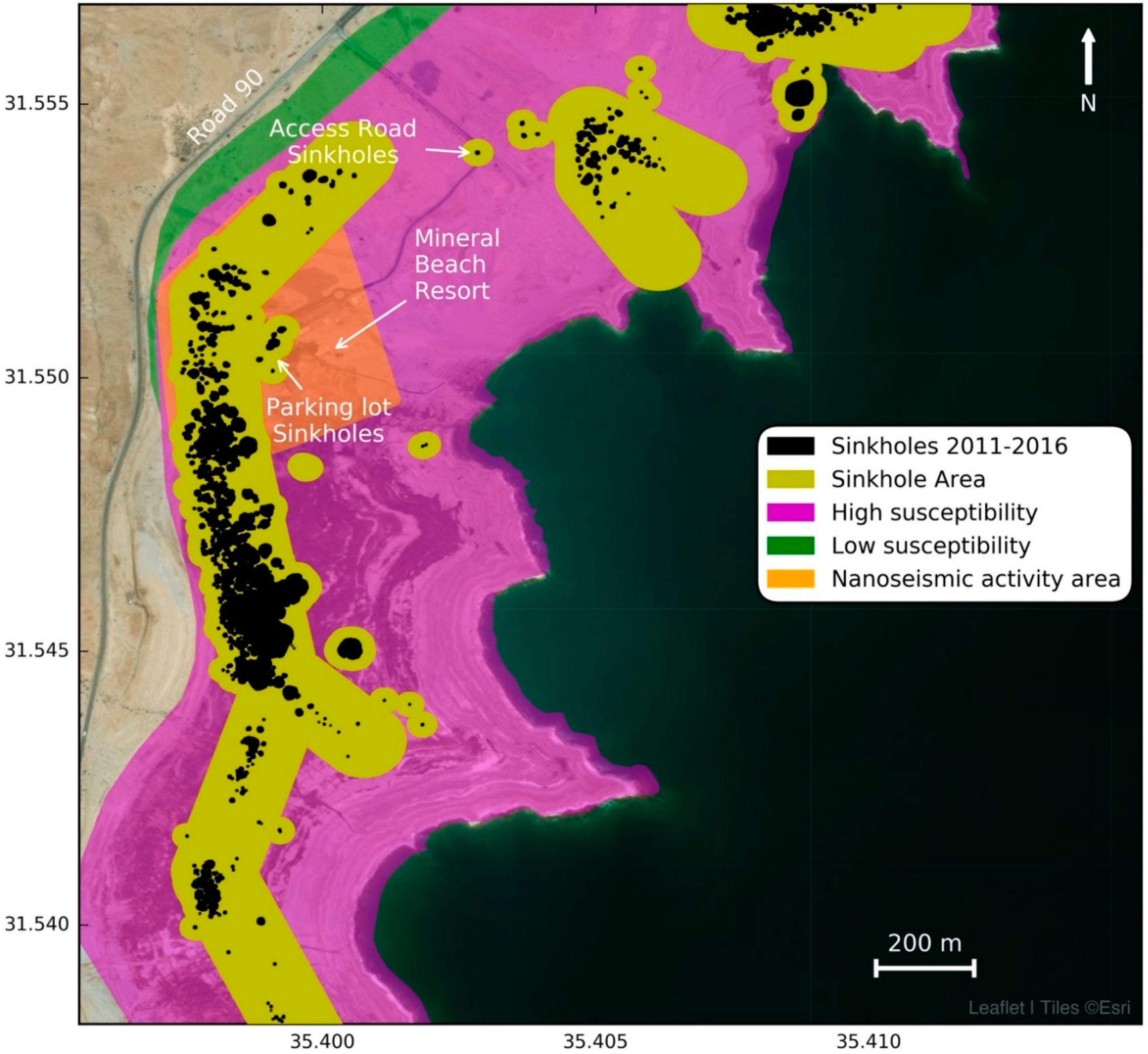
3.4. InSAR and LiDAR Updating of Sinkhole Susceptibility Levels

3.4.1. Sinkhole Susceptibility Maps along the Dead Sea

One of the main sinkhole research products is updated maps of sinkhole susceptibility and potential levels of occurrence. The understanding of the mechanism of sinkhole formation along the DS coast was achieved after years of interdisciplinary research that included borehole analysis, groundwater monitoring, groundwater geochemistry, seismic refraction and reflection, microgravity, electric and electromagnetic methods, and others [15,18,24,26,37]. The main factor controlling the sinkhole potential levels is the spatial extent of the subsurface salt layer, and particularly, its western edge, and the depth of the interface between the saturated and under-saturated groundwater with respect to halite. The estimated extension of the salt layer (marked in magenta in Figure 12) defines the high potential for sinkhole development. Green areas mark areas of low potential due to uncertainty in the salt layer presence. The yellow zones in the susceptibility maps delineate the highest potential for sinkhole development. They were originally constructed at a perpendicular distance of 75 m from a median line drawn along the long axis of the sinkhole cluster or at a radius of 25 m around specific sinkholes. Since 2004, the potential maps have been used by the regional authorities as a mandatory base map for the planning and licensing of new infrastructures.

3.4.2. InSAR Measurements for Updating Sinkhole Susceptibility Levels

The well-established relationships between gradual subsidence and sinkholes calls for a modification of the definition of the highest susceptibility zones from fixed distances around the sinkholes (e.g., Figure 12) to InSAR-detected areas of ongoing subsidence. This adjustment determines the highest susceptibility in a physically justified manner, rather than at arbitrary distances. Furthermore, while active sinkholes remain surrounded by gradual ground subsidence, areas of inactive (old) sinkholes show no subsidence and should no longer be considered to be of a high susceptibility level. Figure 13 illustrates the method used to identify such inactive areas that may be released for public use under certain restrictions. Differential LiDAR measurements may also be used for identifying old inactive sinkholes, but are limited to the availability and uncertainty of the LiDAR data (Figure 13A,B). InSAR measurements (Figure 13C,D) have significantly improved the temporal resolution and sensitivity, allowing the differentiation between active and inactive areas. That said, it should still be pointed out that areas along the DS shore showing no current subsidence by InSAR cannot be automatically ruled out as future potential sinkhole sites and a lag time of a few years should pass before the inactive areas are fully released.

4. Discussion

Several on-demand automatic InSAR processing systems have been recently applied to monitor natural hazards and disasters (e.g., SARVIEWS [38], COMET [39], and ARIA [40]). These systems have been used for the massive processing of InSAR time series (e.g., [41]), rapid damage mapping (e.g., [42]), or natural hazard response (e.g., [43]). With some exceptions of early warning for volcanic eruptions (e.g., [44,45]), most of these systems do not carry a specific precursory component and are in many cases triggered by the event or by other existing hazard alert systems. The case studies presented in this study demonstrate the applicability of semi-automatic InSAR monitoring to early warning, the updating of sinkhole susceptibility maps, and sinkhole hazard assessment and mitigation along the DS in Israel. The implemented monitoring procedure allows for the rapid alert and identification of the increase of immediate hazards within a short time of data acquisition. It also allows for coverage of broad areas rather than individual sites, as nanoseismic monitoring does. In addition, the InSAR displacement time series have been used to analyze the length of sinkhole precursory times and their relationships to subsurface sediment properties, hydrological conditions, and human activities (e.g., [9,12,35,46]), and to define increasing alert levels. Time series algorithms, like Persistent Scatterers (PS, e.g., [47]) or Small BAseline Subsets (SBAS, e.g., [48]) are currently not used for sinkhole monitoring along the DS due to frequent changes in CSK acquisition geometry, which limit the number of consecutive interferograms of the same geometry. Furthermore, in more than 80% of the cases (See Figure 6 in [12]), the collapse occurs in less than six months after the first subsidence, so there is generally insufficient time (number of interferograms) for the PS or SBAS time series. Once the acquisition programming becomes more stable, the use of these algorithms for time-series analysis should be reconsidered.
Our system was able to detect precursory subsidence before the collapse of most sinkholes along the DS, and can be applied for the same use in similar geological settings. However, before implementing this procedure for near-real-time early warning, it is important that the following limitations of the InSAR technique are fully understood.

4.1. InSAR Limitations

4.1.1. Loss of Coherence

A general limitation of the InSAR method is its sensitivity to rapid changes within the scattering targets contained in each pixel, making it impossible to relate the phase difference of two acquisitions to the ground displacement. Our use of a short temporal baseline of ~16 days allowed us to detect subsidence of ~1 mm/day and benefited from low temporal coherence degradation. Slower subsidence rates, however, would require longer time intervals and a risk of higher coherence loss with time. Additionally, heavy rains, flash floods, and large scale human activity (as observed in Ze’elim Fan), would also lead to coherence loss and prevent meaningful InSAR measurements. The X-band SAR wavelength of CSK interferograms commonly results in coherence loss in areas with high vegetation cover. The use of C- or L-band radar systems may help to reduce decorrelation; however, they show a lower sensitivity to ground deformation and are thus less appropriate for the detection of minute subsidence in a timely manner. To overcome the coherence limitations due to the vegetation cover or human-induced surface changes, complementary monitoring methods should be used as described in the Mineral Beach resort example.

4.1.2. Availability of Accurate DEM

The use of high resolution elevation LiDAR measurements for accurate topographic phase removal allowed us to exploit all of the available InSAR pairs including those with perpendicular baselines larger than 1000 m. However, LiDAR measurements are expensive and not available everywhere (e.g., along the border between Israel and Jordan due to flight regulations); they may also require periodic updates in areas of high human activity. The use of high-resolution DEM has been crucial for the effective monitoring of the DS sinkholes (Figure 3) [9], and the lack of an adequate resolution DEM is one of the most serious limitations for the use of CSK data in similar applications.

4.1.3. Technical Limitations

Technical limitations such as SAR acquisition conflicts or temporary telemetry or downlink delays between the satellite platform and the data acquisition system might lead to missing or delayed monitoring data, and more severely, to frequent changes in acquisition geometry, which limit the use of the data with time-series algorithms. These aspects should be taken into account when planning a monitoring campaign for a new region, and normally an acquisition feasibility study is needed to select the best orbits and beams for stable monitoring. The lifespan and availability of the satellite platform should also be taken into account for long-term planning.

4.1.4. Temporal and Spatial Limitation

The InSAR method detects ground deformation occurring during the period spanned by the interferogram. Only sinkholes for which a precursory ground deformation develops over periods longer than the interferometric span (16 days in our case) can be preemptively identified. In areas with a low percentage of cemented gravel along the DS (i.e., mudflats), the entire precursory subsidence may occur within the acquisition interval [12], thus sinkholes cannot be forecasted. However, as the majority of sinkholes, and particularly the deeper and abruptly-forming ones (the most dangerous) occur after subsidence periods of weeks to years, our monitoring procedure is highly appropriate for early warning. Areas showing very low rates of precursory subsidence due to stiff lithology require longer temporal baseline interferograms or time series analysis in order to be effectively captured. Finally, using SAR images with pixel sizes larger than the monitored feature may result in inability to identify the increase in hazards.

4.2. Towards an Automatic Early Warning System

Our Sinkhole Early Warning System is currently semi-automatic, with the interferometric analysis, detection of new subsidence, identification of newly collapsed sinkholes, and general hazard assessment still done manually. Once each new SAR image is acquired, the time needed to evaluate the subsidence signal and verify whether it is indeed precursory, is short (1–2 days). Our next step for the near future is to apply machine learning techniques to the interferometric analysis (e.g., [49]) in order to provide hazard information to stakeholders in an even shorter time.

5. Summary

High resolution InSAR and LiDAR measurements enable the detection of minute precursory subsidence before the catastrophic collapse of sinkholes along the DS shores in Israel. They have also proved to be efficient and well suited for the operational mapping of the zones susceptible to future sinkhole formation. We presented four case studies that illustrate the timelines and effectiveness of our methodology as well as its limitations and complementary methodologies used for sinkhole monitoring and hazard assessment. Our semi-automatic sinkhole early warning system has been operational since 2012 and has on several occasions successfully alerted the local authorities, industry, and governmental agencies before the sinkholes collapsed. While the arid and sparsely populated DS area is almost ideal for monitoring sinkhole hazards, we think that our results and the insights obtained from our monitoring procedure may also prove useful in other sinkhole-prone areas. With the continuous advance in computing power, the use of Artificial Intelligence methods to automatically detect precursory subsidence of sinkhole collapse seems to be achievable in the near future, providing fast early warning alerts to stakeholders for an effective risk reduction.

Author Contributions

Conceptualization, R.N.N., M.A., and G.B.; Methodology, R.N.N., G.B., and M.A.; Software, R.N.N. and Y.M.; Validation, G.B., S.A., and S.S.; Formal Analysis, R.N.N. and Y.M.; Investigation, R.N.N., Y.M., G.B., and E.R.; Resources, G.B., S.A., and S.S.; Data Curation, R.N.N., Y.M., E.R., and M.A.; Writing—Original Draft Preparation, R.N.N. and G.B.; Writing—Review and Editing, M.A., S.A., and S.S.; Visualization, R.N.N.; Supervision, G.B.; Project Administration, G.B.; Funding Acquisition, G.B.

Funding

This research was funded by the Israeli Government under GSI DS project 40702.

Acknowledgments

We would like to thank Assistant Editor Ansley Li, and 4 anonymous reviewers for their thorough and critical reviews which significantly improved this paper. Iyad Swaed is thanked for providing the drone photos. Figures in this article were produced by the Python 2D plotting module Matplotlib [50]. InSAR measurements were carried out using COSMO-SkyMed (CSK®) products, ©ASI (the Italian Space Agency), obtained through an ASI research agreement. InSAR data are available for purchase through e-GEOS (http://www.e-geos.it/products/cosmo.html). The road profile measurements in Figure 7 were provided by the Netivei Israel-National Transport Infrastructure Company.

Conflicts of Interest

The authors declare no conflict of interest. The funders had no role in the design of the study; in the collection, analyses, or interpretation of data; in the writing of the manuscript, or in the decision to publish the results.

References

  1. Galloway, D.; Jones, D.R.; Ingebritsen, S.E. Land Subsidence in the United States; U.S. Department of the Interior; U.S. Geological Survey: Reston, VA, USA, 1999; Volume 1182.
  2. Martinez, J.; Johnson, K.; Neal, J. Sinkholes in Evaporite Rocks. Am. Sci. 1998, 86, 38. [Google Scholar] [CrossRef]
  3. Theron, A.; Engelbrecht, J. The Role of Earth Observation, with a Focus on SAR Interferometry, for Sinkhole Hazard Assessment. Remote Sens. 2018, 10, 1506. [Google Scholar] [CrossRef]
  4. Waltham, T.; Bell, F.G.; Culshaw, M. Sinkholes and Subsidence; Karst and Cavernous Rocks in Engineering and Const; Springer: Berlin/Heidelberg, Germany, 2005; ISBN 978-3-540-20725-2. [Google Scholar]
  5. Parise, M. Rock failures in karst. In Landslides and Engineered Slopes. From the Past to the Future; Cheng, Z., Zhang, J., Li, Z., Wu, F., Ho, K., Eds.; CRC Press: London, UK, 2008; pp. 275–280. ISBN 0780339967. [Google Scholar]
  6. Gutiérrez, F.; Parise, M.; De Waele, J.; Jourde, H. A review on natural and human-induced geohazards and impacts in karst. Earth-Sci. Rev. 2014, 138, 61–88. [Google Scholar] [CrossRef]
  7. Paine, J.G.; Buckley, S.M.; Collins, E.W.; Wilson, C.R. Assessing Collapse Risk in Evaporite Sinkhole-prone Areas Using Microgravimetry and Radar Interferometry. J. Environ. Eng. Geophys. 2012, 17, 75–87. [Google Scholar] [CrossRef]
  8. Nof, R.N. Current Ground Movements in the Dead-Sea Area and Their Implications for Crustal Rheology and Infrastructure Instability: A Synthetic Aperture Radar Interferometry (InSAR) Study. Ph.D. Thesis, Ben-Gurion University of the Negev, Beersheba, Israel, 2012. [Google Scholar]
  9. Nof, R.N.; Baer, G.; Ziv, A.; Raz, E.; Atzori, S.; Salvi, S. Sinkhole precursors along the Dead Sea, Israel, revealed by SAR interferometry. Geology 2013, 41, 1019–1022. [Google Scholar] [CrossRef]
  10. Jones, C.E.; Blom, R.G. Bayou Corne, Louisiana, sinkhole: Precursory deformation measured by radar interferometry. Geology 2014, 42, 111–114. [Google Scholar] [CrossRef]
  11. Intrieri, E.; Gigli, G.; Nocentini, M.; Lombardi, L.; Mugnai, F.; Fidolini, F.; Casagli, N. Sinkhole monitoring and early warning: An experimental and successful GB-InSAR application. Geomorphology 2015, 241, 304–314. [Google Scholar] [CrossRef] [Green Version]
  12. Baer, G.; Magen, Y.; Nof, R.N.; Raz, E.; Lyakhovsky, V.; Shalev, E. InSAR Measurements and Viscoelastic Modeling of Sinkhole Precursory Subsidence: Implications for Sinkhole Formation, Early Warning, and Sediment Properties. J. Geophys. Res. Earth Surf. 2018, 123, 678–693. [Google Scholar] [CrossRef]
  13. Frumkin, A.; Raz, E. Collapse and subsidence associated with salt karstification along the Dead Sea. Carbonates Evaporites 2001, 16, 117–130. [Google Scholar] [CrossRef]
  14. Abelson, M.; Baer, G.; Yechieli, Y. Susceptibility Assessment for Development of Sinkholes along the Western Coast of the Dead Sea—2017 Update; Geological Survey of Israel: Jerusalem, Israel, 2017.
  15. Yechieli, Y.; Abelson, M.; Bein, A.; Crouvi, O.; Shtivelman, V. Sinkhole “swarms” along the Dead Sea cost: Reflection of disturbance of lake and adjacent groundwater systems. Bull. Geol. Soc. Am. 2006, 118, 1075–1087. [Google Scholar] [CrossRef]
  16. Yechieli, Y. Fresh-Saline Ground Water Interface in the Western Dead Sea Area. Ground Water 2000, 38, 615–623. [Google Scholar] [CrossRef]
  17. ESRI Online Map Server. Available online: http://server.arcgisonline.com/arcgis/rest/services/World_Imagery/MapServer/tile/ (accessed on 10 June 2018).
  18. Abelson, M.; Baer, G.; Shtivelman, V.; Wachs, D.; Raz, E.; Crouvi, O.; Kurzon, I.; Yechieli, Y. Collapse-sinkholes and radar interferometry reveal neotectonics concealed within the Dead Sea basin. Geophys. Res. Lett. 2003, 30, 1545. [Google Scholar] [CrossRef]
  19. Ezersky, M. The seismic velocities of Dead Sea salt applied to the sinkhole problem. J. Appl. Geophys. 2006, 58, 45–58. [Google Scholar] [CrossRef]
  20. Baer, G.; Schattner, U.; Wachs, D.; Sandwell, D.; Wdowinski, S.; Frydman, S. The lowest place on Earth is subsiding—An InSAR (interferometric synthetic aperture radar) perspective. Geol. Soc. Am. Bull. 2002, 114, 12–23. [Google Scholar] [CrossRef]
  21. Arkin, Y.; Gilat, A. Dead Sea sinkholes—An ever-developing hazard. Environ. Geol. 2000, 39, 711–722. [Google Scholar] [CrossRef]
  22. Avni, Y.; Lensky, N.; Dente, E.; Shviro, M.; Arav, R.; Gavrieli, I.; Yechieli, Y.; Abelson, M.; Lutzky, H.; Filin, S.; et al. Self-accelerated development of salt karst during flash floods along the Dead Sea Coast, Israel. J. Geophys. Res. Earth Surf. 2016, 121, 17–38. [Google Scholar] [CrossRef]
  23. Shalev, E.; Lyakhovsky, V. Viscoelastic damage modeling of sinkhole formation. J. Struct. Geol. 2012, 42, 163–170. [Google Scholar] [CrossRef]
  24. Abelson, M.; Yechieli, Y.; Crouvi, O.; Baer, G.; Wachs, D.; Bein, A.; Shtivelman, V. Evolution of the Dead Sea sinkholes. Geol. Soc. Am. Spec. Pap. 2006, 401, 241–253. [Google Scholar] [CrossRef]
  25. Abelson, M.; Aksinenko, T.; Kurzon, I.; Pinsky, V.; Baer, G.; Nof, R.; Yechieli, Y. Nanoseismicity forecasts sinkhole collapse in the Dead Sea coast years in advance. Geology 2018, 46, 83–86. [Google Scholar] [CrossRef]
  26. Frumkin, A.; Ezersky, M.; Al-Zoubi, A.; Akkawi, E.; Abueladas, A.-R. The Dead Sea sinkhole hazard: Geophysical assessment of salt dissolution and collapse. Geomorphology 2011, 134, 102–117. [Google Scholar] [CrossRef]
  27. Wust-Bloch, G.H.; Joswig, M. Pre-collapse identification of sinkholes in unconsolidated media at Dead Sea area by “nanoseismic monitoring” (graphical jackknife location of weak sources by few, low-SNR records). Geophys. J. Int. 2006, 167, 1220–1232. [Google Scholar] [CrossRef]
  28. Ezersky, M.G.; Eppelbaum, L.V.; Al-Zoubi, A.; Keydar, S.; Abueladas, A.; Akkawi, E.; Medvedev, B. Geophysical prediction and following development sinkholes in two Dead Sea areas, Israel and Jordan. Environ. Earth Sci. 2013, 70, 1463–1478. [Google Scholar] [CrossRef]
  29. Tachikawa, T.; Hato, M.; Kaku, M.; Iwasaki, A. Characteristics of ASTER GDEM version 2. In Proceedings of the 2011 IEEE International Geoscience and Remote Sensing Symposium, Vancouver, BC, Canada, 24–29 July 2011; pp. 3657–3660. [Google Scholar]
  30. Massonnet, D.; Feigl, K.L. Radar interferometry and its application to changes in the Earth’s surface. Rev. Geophys. 1998, 36, 441–500. [Google Scholar] [CrossRef]
  31. Filin, S.; Baruch, A.; Avni, Y.; Marco, S. Sinkhole characterization in the Dead Sea area using airborne laser scanning. Nat. Hazards 2011, 58, 1135–1154. [Google Scholar] [CrossRef]
  32. GDAL/OGR Contributors GDAL/OGR Geospatial Data Abstraction Software Library, 2018, Open Source Geospatial Foundation. Available online: http://gdal.org (accessed on 10 June 2018).
  33. Wegmuller, U.; Werner, C.; Strozzi, T. SAR interferometric and differential interferometric processing chain. In Proceedings of the 1998 IEEE International Geoscience and Remote Sensing, Seattle, WA, USA, 6–10 July 1998; Volume 2, pp. 1106–1108. [Google Scholar]
  34. Goldstein, R.M.; Werner, C.L. Radar interferogram filtering for geophysical applications. Geophys. Res. Lett. 1998, 25, 4035–4038. [Google Scholar] [CrossRef] [Green Version]
  35. Atzori, S.; Antonioli, A.; Salvi, S.; Baer, G. InSAR-based modeling and analysis of sinkholes along the Dead Sea coastline. Geophys. Res. Lett. 2015, 42, 8383–8390. [Google Scholar] [CrossRef]
  36. Ezersky, M.; Legchenko, A.; Camerlynck, C.; Al-Zoubi, A.; Eppelbaum, L.; Keydar, S.; Boucher, M.; Chalikakis, K. The Dead Sea sinkhole hazard—New findings based on a multidisciplinary geophysical study. Z. Geomorphol. Suppl. Issues 2010, 54, 69–90. [Google Scholar] [CrossRef]
  37. Ezersky, M.; Legchenko, A.; Camerlynck, C.; Al-Zoubi, A. Identification of sinkhole development mechanism based on a combined geophysical study in Nahal Hever South area (Dead Sea coast of Israel). Environ. Geol. 2009, 58, 1123–1141. [Google Scholar] [CrossRef]
  38. SARVIEWS. Available online: http://sarviews-hazards.alaska.edu/ (accessed on 9 December 2018).
  39. COMET. Available online: http://comet.nerc.ac.uk/COMET-LiCS-portal/ (accessed on 9 December 2018).
  40. ARIA. Available online: https://aria.jpl.nasa.gov/ (accessed on 9 December 2018).
  41. De Luca, C.; Zinno, I.; Manunta, M.; Lanari, R.; Casu, F. Large areas surface deformation analysis through a cloud computing P-SBAS approach for massive processing of DInSAR time series. Remote Sens. Environ. 2017, 202, 3–17. [Google Scholar] [CrossRef]
  42. Yun, S.-H.; Hudnut, K.; Owen, S.; Webb, F.; Simons, M.; Sacco, P.; Gurrola, E.; Manipon, G.; Liang, C.; Fielding, E.; et al. Rapid Damage Mapping for the 2015 M w 7.8 Gorkha Earthquake Using Synthetic Aperture Radar Data from COSMO–SkyMed and ALOS-2 Satellites. Seismol. Res. Lett. 2015, 86, 1549–1556. [Google Scholar] [CrossRef] [Green Version]
  43. Milillo, P.; Riel, B.; Minchew, B.; Yun, S.-H.; Simons, M.; Lundgren, P. On the Synergistic Use of SAR Constellations’ Data Exploitation for Earth Science and Natural Hazard Response. IEEE J. Sel. Top. Appl. Earth Obs. Remote Sens. 2016, 9, 1095–1100. [Google Scholar] [CrossRef]
  44. Dzurisin, D. A comprehensive approach to monitoring volcano deformation as a window on the eruption cycle. Rev. Geophys. 2003, 41, 1–29. [Google Scholar] [CrossRef]
  45. Meyer, F.J.; McAlpin, D.B.; Gong, W.; Ajadi, O.; Arko, S.; Webley, P.W.; Dehn, J. Integrating SAR and derived products into operational volcano monitoring and decision support systems. ISPRS J. Photogramm. Remote Sens. 2015, 100, 106–117. [Google Scholar] [CrossRef]
  46. Shviro, M.; Haviv, I.; Baer, G. High-resolution InSAR constraints on flood-related subsidence and evaporite dissolution along the Dead Sea shores: Interplay between hydrology and rheology. Geomorphology 2017, 293, 53–68. [Google Scholar] [CrossRef]
  47. Ferretti, A.; Prati, C.; Rocca, F. Permanent scatterers in SAR interferometry. IEEE Trans. Geosci. Remote Sens. 2001, 39, 8–20. [Google Scholar] [CrossRef] [Green Version]
  48. Berardino, P.; Fornaro, G.; Lanari, R.; Sansosti, E. A new algorithm for surface deformation monitoring based on small baseline differential SAR interferograms. IEEE Trans. Geosci. Remote Sens. 2002, 40, 2375–2383. [Google Scholar] [CrossRef]
  49. Schwegmann, C.P.; Kleynhans, W.; Engelbrecht, J.; Mdakane, L.W.; Meyer, R.G.V. Subsidence feature discrimination using deep convolutional neural networks in synthetic aperture radar imagery. In Proceedings of the 2017 IEEE International Geoscience and Remote Sensing Symposium (IGARSS), Fort Worth, TX, USA, 23–28 July 2017; pp. 4626–4629. [Google Scholar]
  50. Hunter, J.D. Matplotlib: A 2D graphics environment. Comput. Sci. Eng. 2007, 9, 90–95. [Google Scholar] [CrossRef]
Figure 1. Location maps. (A) Regional context of the Dead Sea area (marked as a white rectangle); (B) The Dead Sea area with sinkholes formed between 2011 and 2016 (red) and sites elaborated in this research. Background obtained from the ESRI online map server [17].
Remotesensing 11 00089 g001
Figure 2. Cumulative number of sinkholes from 1980 to 2016 (red line) and the 1976–2018 Dead Sea water levels (blue line).
Remotesensing 11 00089 g002
Figure 3. A comparison of two interferograms of the same period (111214–111230) with a 680 m perpendicular baseline using: (A) Combined ASTER - LiDAR DEM; and (B) ASTER GDEM alone.
Remotesensing 11 00089 g003
Figure 4. Monitoring system workflow.
Remotesensing 11 00089 g004
Figure 5. An example of the alerting procedure, Hever site (Figure 1). (A) Hill-shaded relief of the May 2011 LiDAR DSM showing mapped sinkholes up to 2011 (red polygons), cross section B-B’ location (white line), and the area of panels C-H (dashed white rectangle); (B) 111214–111230 (YYMMDD) interferogram of the same area as panel A, showing subsidence related to the existing sinkholes in the NW corner and no subsidence along profile B-B’. The alert level is green; (C) 111230–120216 interferogram (48 days due to acquisition gaps) showing new subsidence along B-B’. The alert level is raised to yellow; (D) The consecutive 16-day interferogram, showing almost identical subsidence rate; (E) 120319–120404 interferogram showing accelerated subsidence. Alert level is raised to orange; (F) 120404–120420 interferogram showing continued subsidence acceleration; (G) 120522–120607 interferogram showing de-correlation at the center and margins of the subsiding area, presumably due to sinkhole collapse. Alert level is raised to red; (H) Hill-shaded relief of the May 2013 LiDAR DSM showing mapped sinkholes up to 2011 (red polygons) a new sinkhole that coincides with the location of the de-correlated area in G (dashed blue circle) and sinkholes that formed between June 2012 and May 2013 (unmarked); (I) First appearance of the sinkhole, photographed on June 7, 2012; (J) Cumulative displacement along profile B-B’; (K) Time series of cumulative maximum displacement along profile B-B’. Colors correspond to alert level.
Remotesensing 11 00089 g005
Figure 6. (A) Location map of Road 90, En Gedi. Dashed white rectangle marks the area covered in panel B. (B) Interferogram 111214–111230 (YYMMDD) showed no subsidence at the intersection between the road and the subsiding lineament (solid white circle). The rectangle marks the area covered in panels C–F. (C)–(F) interferograms (date convention as above) showing the beginning and acceleration of subsidence on the road. Interferograms are projected over hill-shaded relief of LiDAR DSM. Panel A background was obtained from the ESRI online map server [17].
Remotesensing 11 00089 g006
Figure 7. Maximum LOS displacement rates (black marks, covering interferometric span) at the point of highest displacement along cross section A-A’, Road 90 (Figure 6D). Gray areas mark periods of incoherent interferograms. The green dotted line marks the leveling measurements provided by the NTIC and converted to LOS for the incidence angle of 40°. The yellow arrow marks the interferogram of identified new subsidence. The time when the alert was issued to the regional authorities and the roads company is marked by the orange arrow. Blue arrows mark the collapse times of sinkholes at the road margins (see also Figure 8D). The red arrow marks the time of sinkhole detection directly beneath the road.
Remotesensing 11 00089 g007
Figure 8. Road 90 sinkholes near En Gedi. Picture dates are labeled YYMMDD with look direction in brackets. For relative location, see panel (D). (A) Sinkholes west of the road (A1), after being filled with gravel; (B) Exposure of the geosynthetic sheet above a 5 m wide, 9 m deep cavity (B1); (C) sinkhole collapse on the road (C1), after almost five years of InSAR-detected subsidence; (D) Drone photo of the subsidence area. Note the circular cracks (D1) surrounding the subsidence center (E1). Blue circles mark sinkholes along the road margins and red circles mark sinkholes collapsed along the road; (E) Compressional deformation on road asphalt at the center of the subsiding area (E1).
Remotesensing 11 00089 g008
Figure 9. Ze’elim Fan. (A) Sinkholes formed between 2011 and 2016 (marked in red). Suggested and final location for the pumping station (P9) are marked as open and closed circles, respectively; (B) interferogram 130423–130509 (16 days) showing subsidence in the areas west of the two southern sites, where the pipelines were planned, and a relatively stable area west of the northern site; (C) A drone photo of the current construction works at P9 site (look to the south).
Remotesensing 11 00089 g009
Figure 10. Mineral Beach resort. (A) Location map. Sinkholes formed between 2011 and 2016 are marked in black; (B) interferogram 140617–140703 (16 days) showing subsidence near the access road and typical decorrelation in the resort area due to vegetation and human activity. Subsidence is also visible along the sinkhole lineament north and west of the resort area. White circles mark the nanoseismic epicenters. (C) Drone photo of the access road sinkhole; (D) The access road sinkholes (look to the east); (E) Southward looking drone photo of the parking lot sinkholes and the sinkhole lineament.
Remotesensing 11 00089 g010
Figure 11. Time series of maximum LOS displacement rates along the access road to the Mineral Beach site. Dark lines mark the displacement rate for the interferometric time span. Gray areas mark periods of incoherent interferometric signal. The yellow arrow marks the time of the alert to the regional council engineer; the orange arrow marks the time of subsidence acceleration; the red arrow marks the time of the first sinkhole collapse near the road.
Remotesensing 11 00089 g011
Figure 12. Sinkhole susceptibility map of the Mineral Beach area. See text for more details.
Remotesensing 11 00089 g012
Figure 13. Identification of temporal change from active to inactive areas. The dashed line in all panels marks the border between the 2017 InSAR-mapped active and inactive areas (east and west of the line, respectively). (A) Hill-shaded relief of 2012 LiDAR DSM, showing old inactive sinkholes south of En Gedi; (B) Hill-shaded relief of 2017 LiDAR DSM tinted by elevation changes between 2017 and 2012. The LiDAR DSM is masked at the 2012 Dead Sea shoreline; (C) 120216–120303 interferogram, showing active areas both east and west of the dashed line; (D) 170831–170916 interferogram, showing active areas only east of the line.
Remotesensing 11 00089 g013

