Evaluation of SMAP Freeze/Thaw Retrieval Accuracy at Core Validation Sites in the Contiguous United States

 ,
,  ,
, 
Abstract
1. Introduction
2. Data and Processing
2.1. SMAP Radiometer Data (L3_SM_P, Version 4)
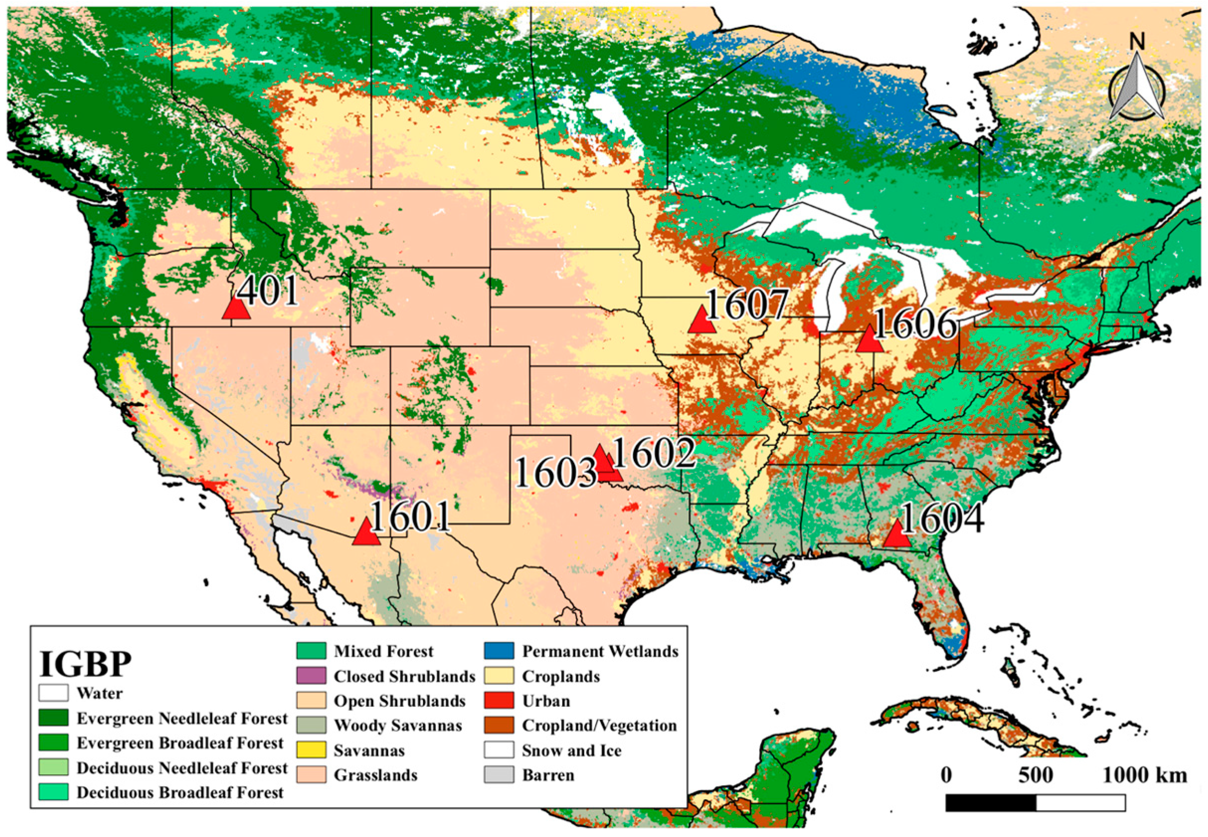
2.2. Data Processing and Selection of Test Sites
2.3. Idaho, Iowa, and Indiana SMAP Grid Attributes
3. Methods
3.1. FT Algorithm
3.2. Classification Accuracy
3.3. Assessment of Factors That Impact SMAP Retrieval Accuracy
3.3.1. Data Aggregation Scheme
3.3.2. Temporal Subsets
3.3.3. NPR Threshold
3.3.4. Sampling Error
4. Results
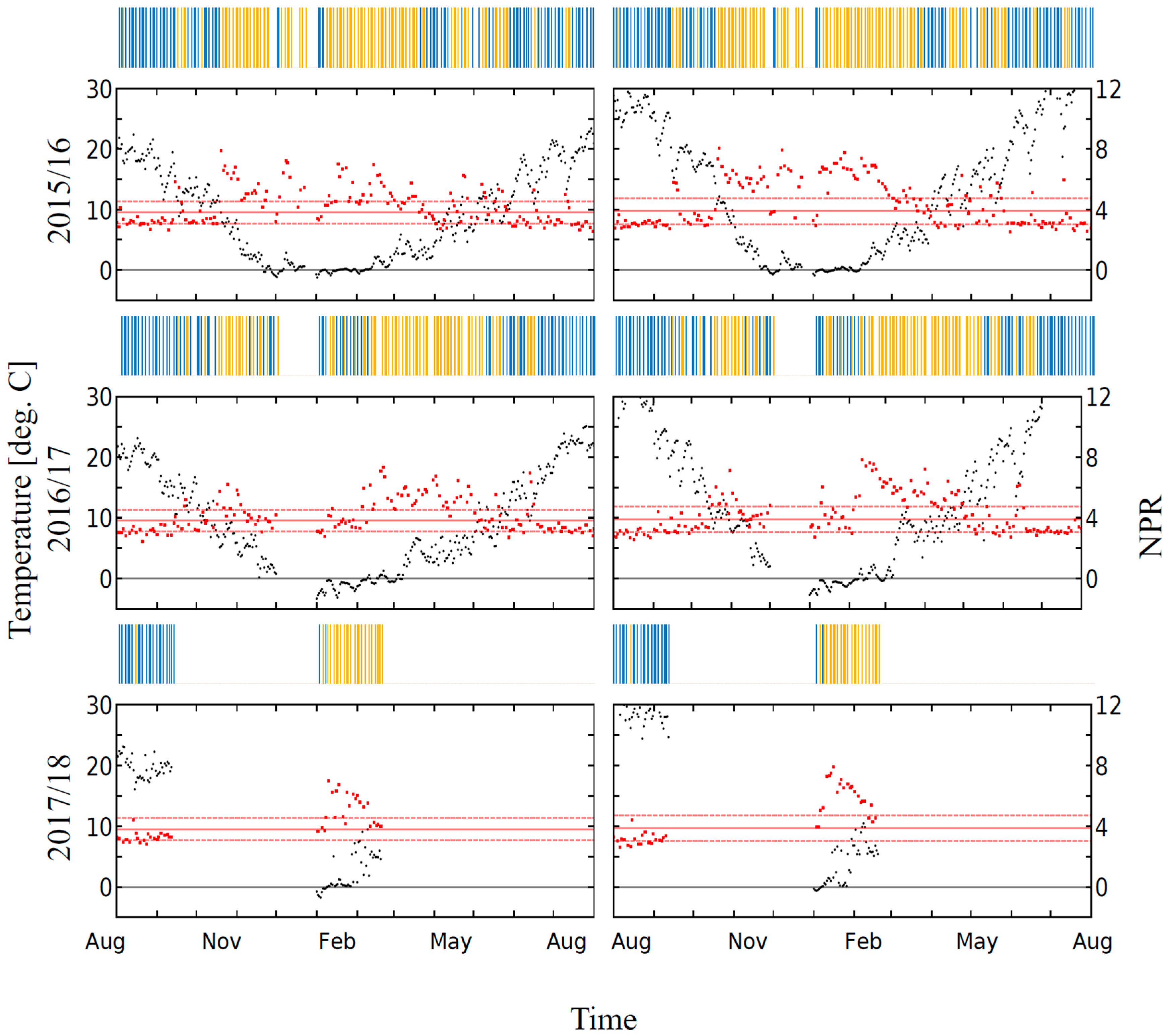
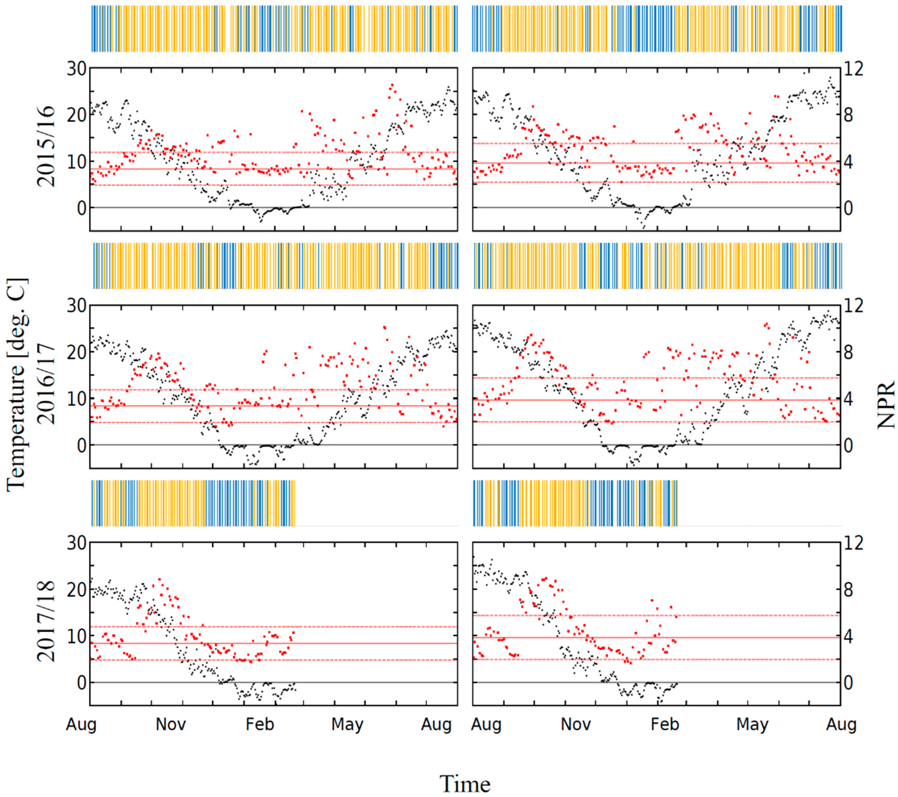
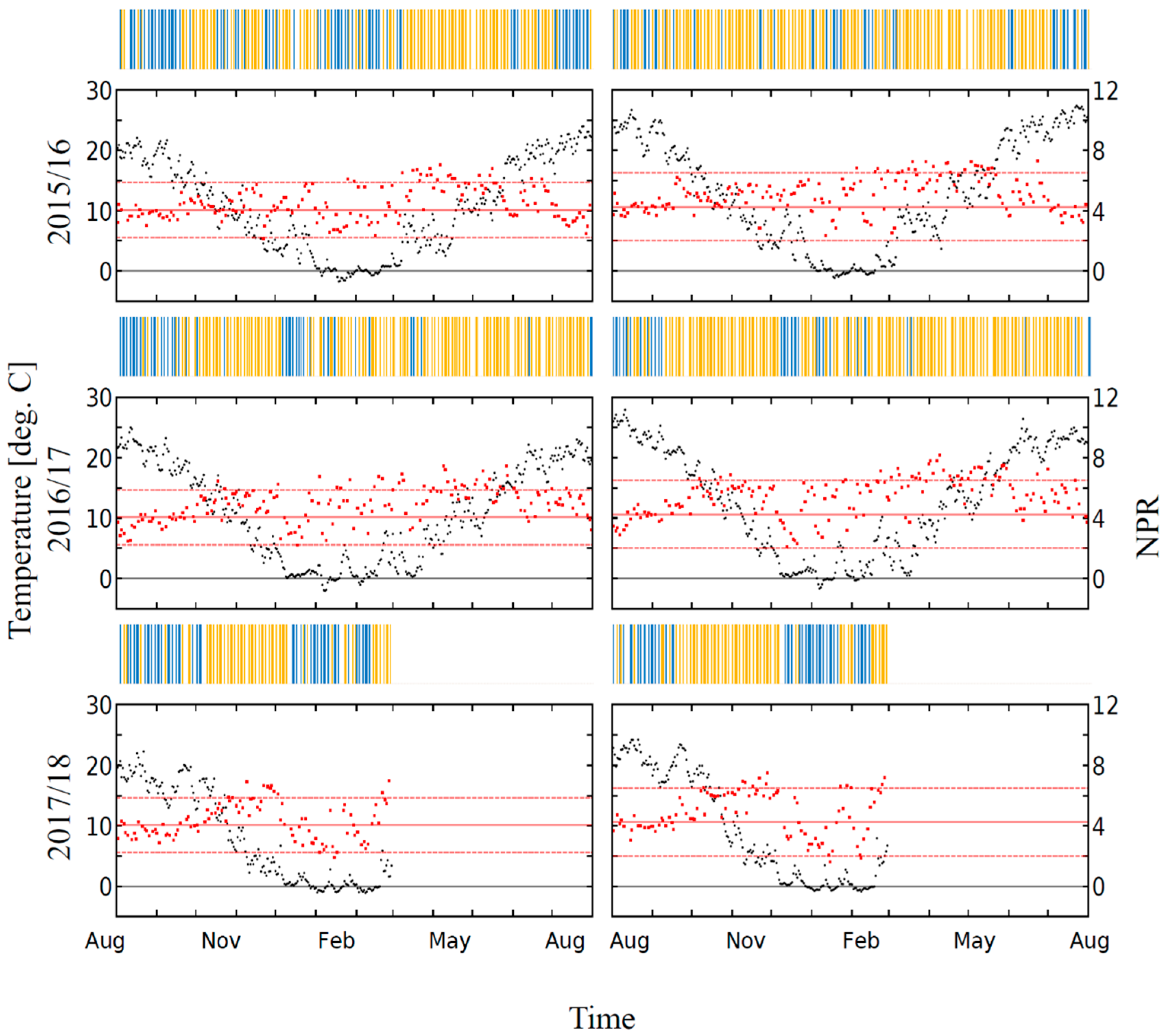
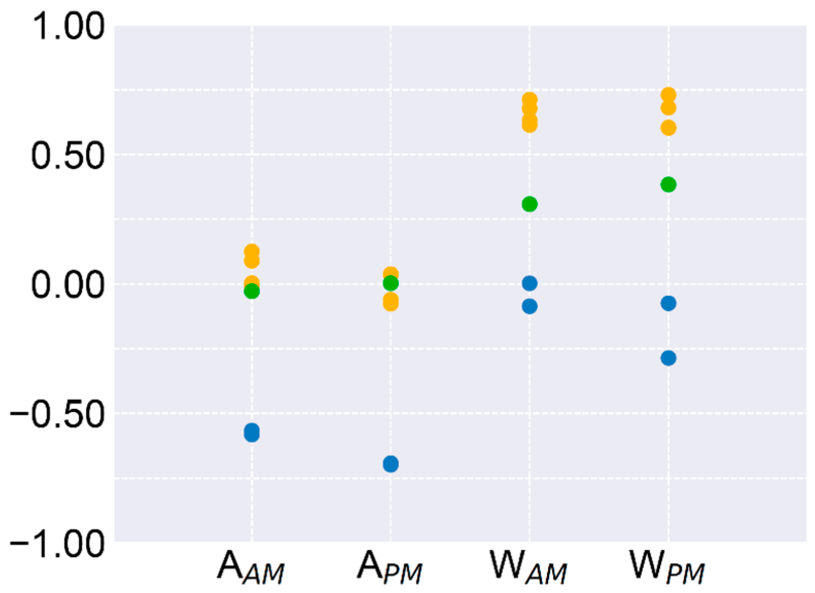
4.1. Freeze and Thaw References Values
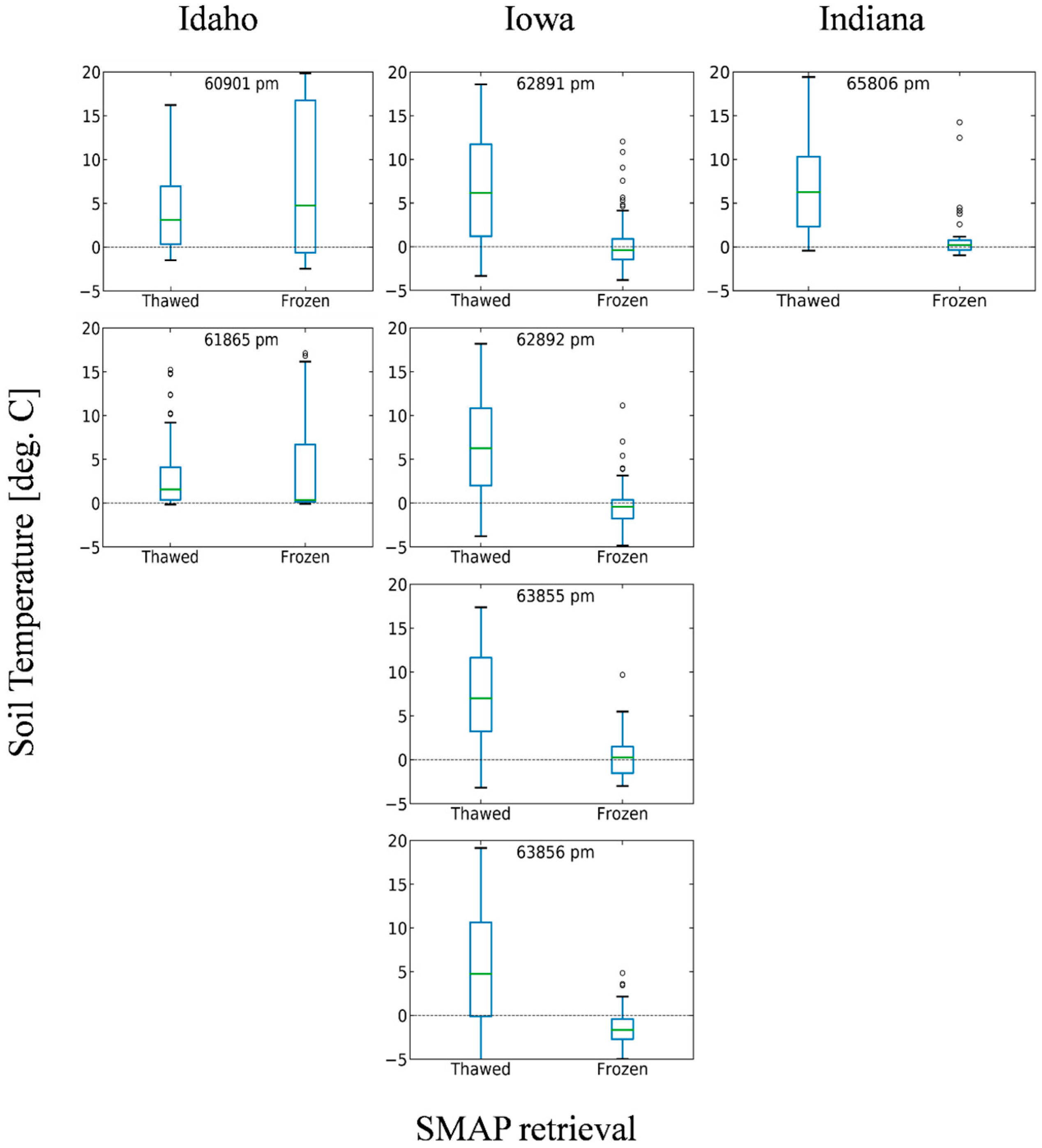
4.2. SMAP FT Correspondence with In Situ Data
4.3. SMAP FT Retrieval Accuracy by Grid
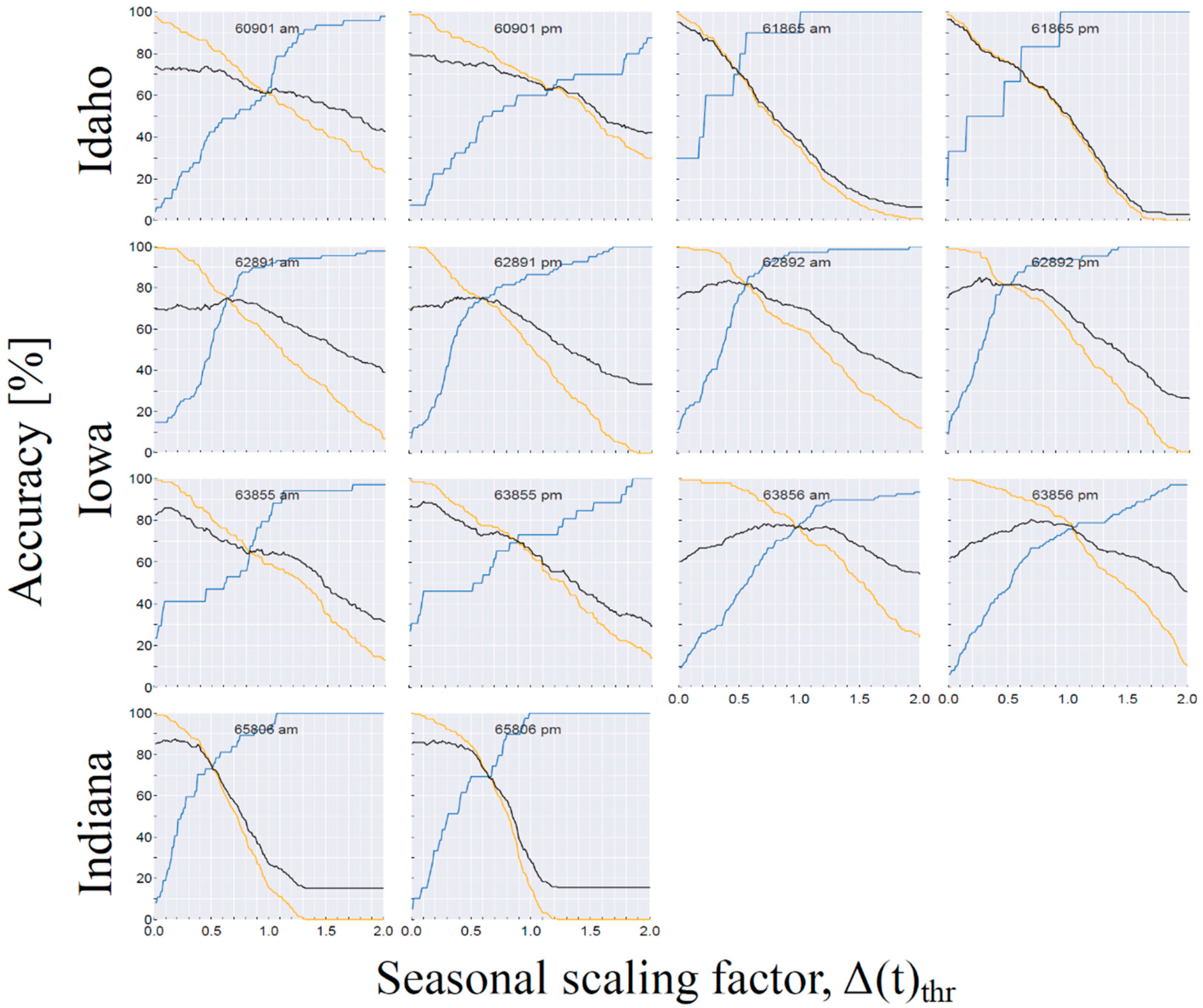
4.4. Accuracy Metrics as Function of Δ(t)thr
4.5. Estimation of In Situ Sampling Error
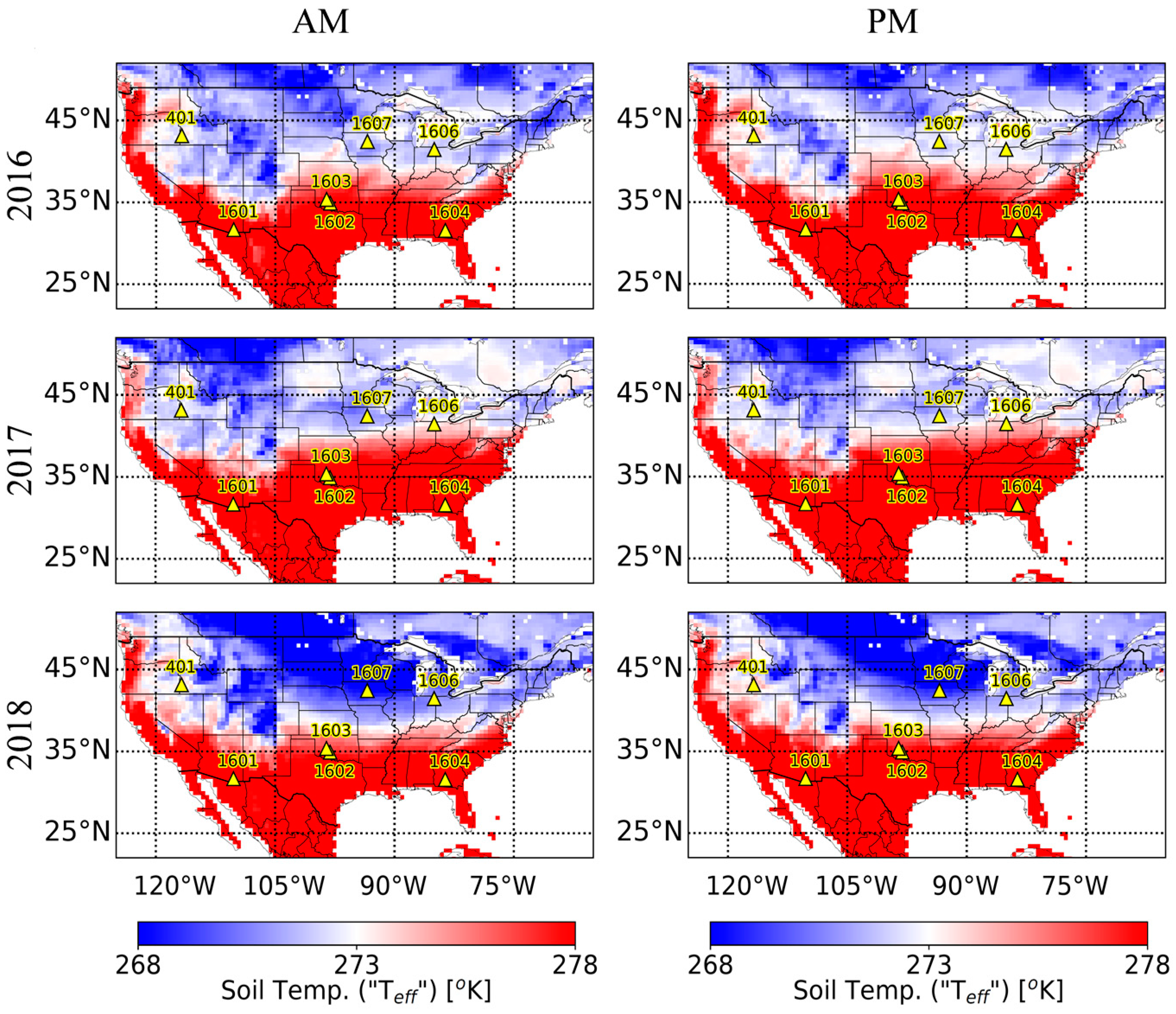
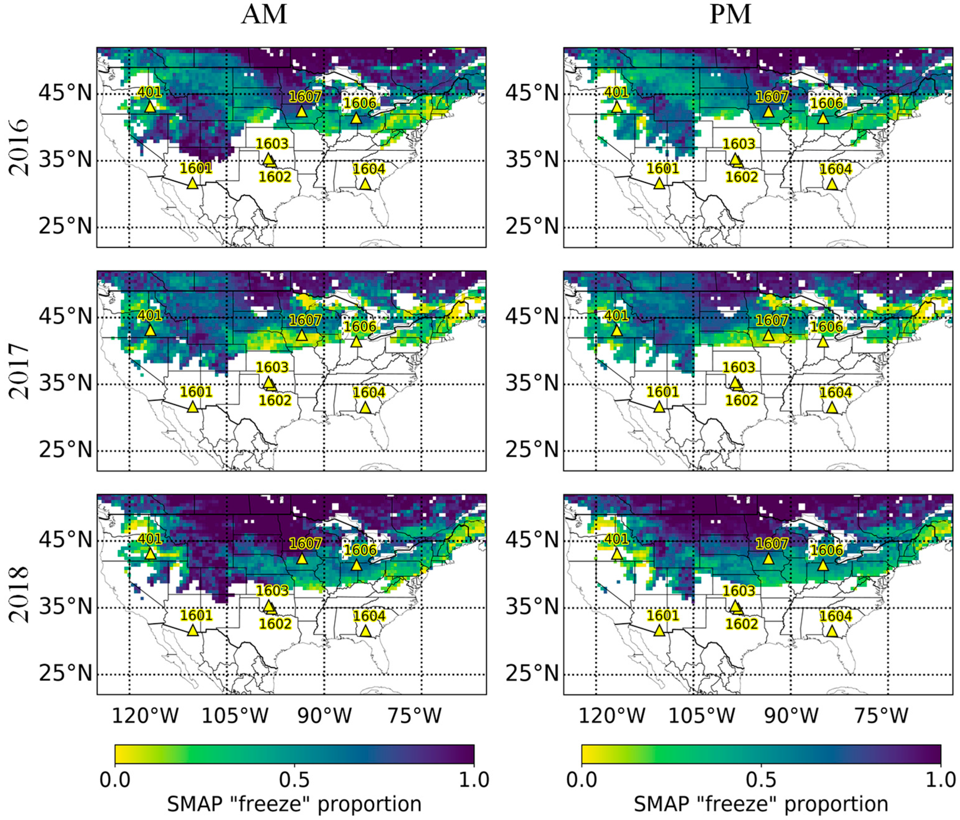
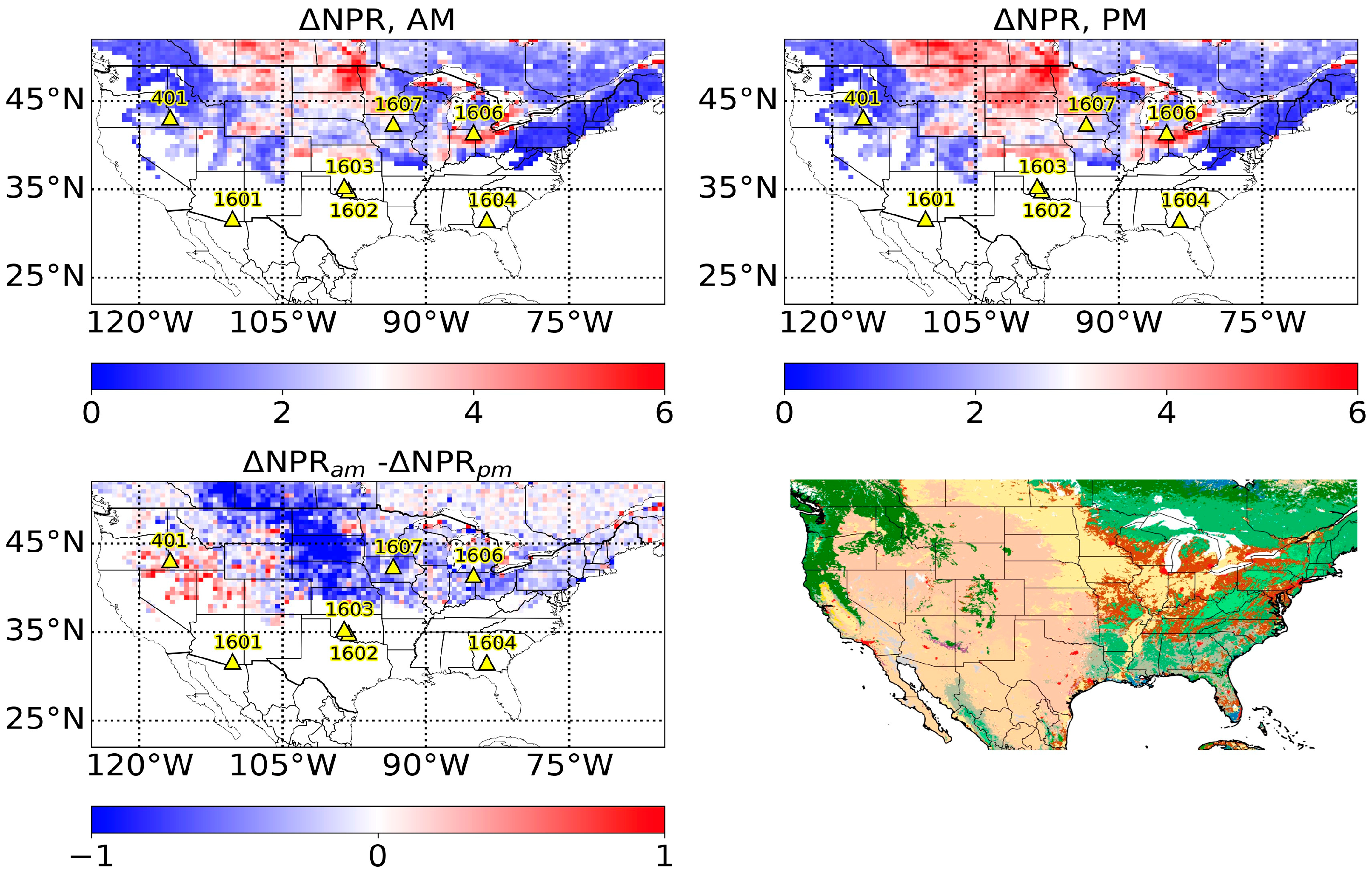
4.6. CONUS FT Extent from L3_SM_P
5. Discussion
6. Summary and Conclusions
Author Contributions
Acknowledgments
Conflicts of Interest
References
- Zhang, T. Investigation of the near-surface soil freeze-thaw cycle in the contiguous United States: Algorithm development and validation. J. Geophys. Res. 2003, 108, 8860. [Google Scholar] [CrossRef]
- Colliander, A.; McDonald, K.; Zimmermann, R.; Schroeder, R.; Kimball, J.S.; Njoku, E.G. Application of quikSCAT backscatter to SMAP validation planning: Freeze/Thaw state over ALECTRA sites in Alaska from 2000 to 2007. IEEE Trans. Geosci. Remote Sens. 2012, 50, 461–468. [Google Scholar] [CrossRef]
- Entekhabi, D.; Yueh, S.; O’Neill, P.E.; Kellogg, K.H.; Allen, A.; Bindlish, R.; Brown, M.; Chan, S.; Colliander, A.; Crow, W.T. SMAP Handbook; JPL: Pasadena, CA, USA, 2014.
- Kim, Y.; Kimball, J.S.; Mcdonald, K.C.; Member, S.; Glassy, J. Developing a Global Data Record of Daily Landscape Freeze/Thaw Status Using Satellite Passive Microwave Remote Sensing. IEEE Trans. Geosci. Remote Sens. 2011, 49, 949–960. [Google Scholar] [CrossRef]
- Kimball, J.S.; McDonald, K.C.; Frolking, S.; Running, S.W. Radar remote sensing of the spring thaw transition across a boreal landscape. Remote Sens. Environ. 2004, 89, 163–175. [Google Scholar] [CrossRef]
- Zwieback, S.; Paulik, C.; Wagner, W. Frozen soil detection based on advanced scatterometer observations and air temperature data as part of soil moisture retrieval. Remote Sens. 2015, 7, 3206–3231. [Google Scholar] [CrossRef]
- Du, J.; Kimball, J.S.; Azarderakhsh, M.; Dunbar, R.S.; Moghaddam, M.; McDonald, K.C. Classification of Alaska spring thaw characteristics using satellite L-band radar remote sensing. IEEE Trans. Geosci. Remote Sens. 2015, 53, 542–556. [Google Scholar]
- Pastick, N.J.; Jorgenson, M.T.; Wylie, B.K.; Nield, S.J.; Johnson, K.D.; Finley, A.O. Distribution of near-surface permafrost in Alaska: Estimates of present and future conditions. Remote Sens. Environ. 2015, 168, 301–315. [Google Scholar] [CrossRef]
- Cherkauer, K.A.; Lettenmaier, D.P. Hydrologic effects of frozen soils in the upper Mississippi River basin. J. Geophys. Res. Atmos. 1999, 104, 19599–19610. [Google Scholar] [CrossRef]
- Campbell, J.L.; Ollinger, S.V.; Flerchinger, G.N.; Wicklein, H.; Hayhoe, K.; Bailey, A.S. Past and projected future changes in snowpack and soil frost at the Hubbard Brook Experimental Forest, New Hampshire, USA. Hydrol. Process. 2010, 24, 2465–2480. [Google Scholar] [CrossRef]
- Ovik, J.M.; Siekmeier, J.A.; Van Deusen, D.A. Improved Spring Load Restriction Guidelines Using Mechanistic Analysis; Minnesota DOT Report No. 2000-18; Minnesota Department of Transportation: Saint Paul, MN, USA, 2000.
- Judge, J.; Member, S.; Galantowicz, J.F.; England, A.W.; Dahl, P. Freeze/Thaw Classification for Prairie Soils Using SSM/I Radiobrightnesses. IEEE Trans. Geosci. Remote Sens. 1997, 35, 827–832. [Google Scholar] [CrossRef]
- Rautiainen, K.; Lemmetyinen, J.; Pulliainen, J.; Vehvilainen, J.; Drusch, M.; Kontu, A.; Kainulainen, J.; Seppänen, J. L-band radiometer observations of soil processes in boreal and subarctic environments. IEEE Trans. Geosci. Remote Sens. 2012, 50, 1483–1497. [Google Scholar] [CrossRef]
- Kalantari, P.; Bernier, M.; McDonald, K.C.; Poulin, J. Using available time series of Passive and Active Microwave to develop SMAP Freeze/Thaw algorithms adapted for the canadian subarctic. In Proceedings of the 2014 IEEE International Geoscience and Remote Sensing Symposium (IGARSS), Quebec City, QC, Canada, 13–18 July 2014; pp. 2550–2553. [Google Scholar]
- Roy, A.; Royer, A.; Derksen, C.; Brucker, L.; Langlois, A.; Mialon, A.; Kerr, Y.H. Evaluation of spaceborne L-band radiometer measurements for terrestrial freeze/thaw retrievals in Canada. IEEE J. Sel. Top. Appl. Earth Obs. Remote Sens. 2015, 8, 4442–4459. [Google Scholar] [CrossRef]
- Rautiainen, K.; Lemmetyinen, J.; Schwank, M.; Kontu, A.; Ménard, C.B.; Mätzler, C.; Drusch, M.; Wiesmann, A.; Ikonen, J.; Pulliainen, J. Detection of soil freezing from L-band passive microwave observations. Remote Sens. Environ. 2014, 147, 206–218. [Google Scholar] [CrossRef]
- Rautiainen, K.; Parkkinen, T.; Lemmetyinen, J.; Schwank, M.; Wiesmann, A.; Ikonen, J.; Derksen, C.; Davydov, S.; Davydova, A.; Boike, J. SMOS prototype algorithm for detecting autumn soil freezing. Remote Sens. Environ. 2016, 180, 346–360. [Google Scholar] [CrossRef]
- Kim, Y.; Kimball, J.S.; Glassy, J.; Du, J. An extended global Earth system data record on daily landscape freeze–thaw status determined from satellite passive microwave remote sensing. Earth Syst. Sci. Data 2017, 9, 133–147. [Google Scholar] [CrossRef]
- Derksen, C.; Xu, X.; Scott Dunbar, R.; Colliander, A.; Kim, Y.; Kimball, J.S.; Black, T.A.; Euskirchen, E.; Langlois, A.; Loranty, M.M.; et al. Retrieving landscape freeze/thaw state from Soil Moisture Active Passive (SMAP) radar and radiometer measurements. Remote Sens. Environ. 2017, 194, 48–62. [Google Scholar] [CrossRef]
- Li, X.; McColl, K.A.; Lyu, H.; Xu, X.; Derksen, C.; Lu, H.; Entekhabi, D. Validation of the SMAP freeze/thaw product using categorical triple collocation. Int. Geosci. Remote Sens. Symp. 2017, 205, 1596–1598. [Google Scholar] [CrossRef]
- Jackson, T.; Colliander, A.; Kimball, J.; Reichle, R.; Crow, W.; Entekhabi, D.; O’Neill, P.; Njoku, E. SMAP Science Data Calibration and Validation Plan; JPL D-52544; JPL: Pasadena, CA, USA, 2012.
- Brodzik, M.J.; Billingsley, B.; Haran, T.; Raup, B.; Savoie, M.H. EASE-Grid 2.0: Incremental but Significant Improvements for Earth-Gridded Data Sets. ISPRS Int. J. Geo-Inf. 2012, 1, 32–45. [Google Scholar] [CrossRef]
- Brodzik, M.; Billingsley, B.; Haran, T.; Raup, B.; Savoie, M. Correction: EASE-Grid 2.0: Incremental but Significant Improvements for Earth-Gridded Data Sets. ISPRS Int. J. Geo-Inf. 2014, 3, 1154–1156. [Google Scholar] [CrossRef]
- Chan, S.; Bindlish, R.; O’Neill, P.; Jackson, T.; Chaubell, J.; Piepmeier, J.; Dunbar, S.; Colliander, A.; Chen, F.; Entekhabi, D.; et al. Development and validation of the SMAP enhanced passive soil moisture product. In Proceedings of the 2017 IEEE International Geoscience and Remote Sensing Symposium (IGARSS), Fort Worth, TX, USA, 23–28 July 2017; pp. 2539–2542. [Google Scholar] [CrossRef]
- Chan, S.K.; Bindlish, R.; O’Neill, P.; Jackson, T.; Njoku, E.; Dunbar, S.; Chaubell, J.; Piepmeier, J.; Yueh, S.; Entekhabi, D. Development and assessment of the SMAP enhanced passive soil moisture product. Remote Sens. Environ. 2018, 204, 931–941. [Google Scholar] [CrossRef]
- Colliander, A.; Jackson, T.J.; Chan, S.K.; O’Neill, P.; Bindlish, R.; Cosh, M.H.; Caldwell, T.; Walker, J.P.; Berg, A.; McNairn, H.; et al. An assessment of the differences between spatial resolution and grid size for the SMAP enhanced soil moisture product over homogeneous sites. Remote Sens. Environ. 2018, 207, 65–70. [Google Scholar] [CrossRef]
- O’Neill, P.E.; Chan, S.; Njoku, E.G.; Jackson, T.; Bindlish, R. SMAP L3 Radiometer Global Daily 36 km EASE-Grid Soil Moisture, Version 4. Available online: http://nsidc.org/data/SPL3SMP (accessed on 1 January 2018).
- Chan, S.K.; Bindlish, R.; O’Neill, P.E.; Njoku, E.; Jackson, T.; Colliander, A.; Chen, F.; Burgin, M.; Dunbar, S.; Piepmeier, J.; et al. Assessment of the SMAP Passive Soil Moisture Product. IEEE Trans. Geosci. Remote Sens. 2016, 54, 4994–5007. [Google Scholar] [CrossRef]
- SMAP Algorithm Development Team. SMAP Sience Team SMAP Ancillary Data Report on Surface Temperature. Available online: http://smap.jpl.nasa.gov/system/internal_ resources/details/original/293_051_surf_temp_150304.pdf (accessed on 4 January 2018).
- Chan, S. SMAP Ancillary Data Report on Static Water Fraction; Jet Propuls. Lab., Calif. Inst. Technol.: Pasadena, CA, USA, 2013.
- Colliander, A.; Jackson, T.J.; Bindlish, R.; Chan, S.; Das, N.; Kim, S.B.; Cosh, M.H.; Dunbar, R.S.; Dang, L.; Pashaian, L.; et al. Validation of SMAP surface soil moisture products with core validation sites. Remote Sens. Environ. 2017, 191, 215–231. [Google Scholar] [CrossRef]
- Peel, M.C.; Finlayson, B.L.; McMahon, T.A. Updated world map of the Köppen-Geiger climate classification. Hydrol. Earth Syst. Sci. Discuss. 2007, 4, 439–473. [Google Scholar] [CrossRef]
- Dunbar, S.; Xu, X.; Colliander, A.; Derksen, C.; Kimball, J.; Kim, Y. SMAP Level 3 Radiometer Freeze/Thaw Data Products. Available online: https://nsidc.org/sites/nsidc.org/files/technical-references/L3_FT_P_ATBD_v7.pdf (accessed on 12 January 2018).
- Xu, X.; Dunbar, S.; Derksen, C.; Colliander, A.; Kim, Y.; Kimball, J.S. SMAP L3 Radiometer Northern Hemisphere Daily 36 km EASE-Grid Freeze/Thaw State, Version 1. Available online: http://nsidc.org/data/SPL3FTP (accessed on 4 January 2018).
- Schroeder, R.; McDonald, K.C.; Chapman, B.D.; Jensen, K.; Podest, E.; Tessler, Z.D.; Bohn, T.J.; Zimmermann, R. Development and evaluation of a multi-year fractional surface water data set derived from active/passive microwave remote sensing data. Remote Sens. 2015, 7, 16688–16732. [Google Scholar] [CrossRef]
- Owe, M.; de Jeu, R.; Walker, J. A methodology for surface soil moisture and vegetation optical depth retrieval using the microwave polarization difference index. IEEE Trans. Geosci. Remote Sens. 2001, 39, 1643–1654. [Google Scholar] [CrossRef]
- Artemov, V.G.; Volkov, A.A. Water and ice dielectric spectra scaling at 0 C. Ferroelectrics 2014, 466, 158–165. [Google Scholar] [CrossRef]
- Xu, X.; Dunbar, R.S.; Derksen, C.; Colliander, A.; Kim, Y.; Kimball, S. SMAP L3 Radiometer Northern Hemisphere Daily 36 km EASE-Grid Freeze/Thaw State, Version 2. Available online: https://nsidc.org/data/spl3ftp (accessed on 8 June 2018).
- Shepherd, A.; McGinn, S.M. Assessment of climate change on the Canadian prairies from downscaled GCM data. Atmos. Ocean 2003, 41, 301–316. [Google Scholar] [CrossRef]
- Schwank, M.; Rautiainen, K.; Mätzler, C.; Stähli, M.; Lemmetyinen, J.; Pulliainen, J.; Vehviläinen, J.; Kontu, A.; Ikonen, J.; Ménard, C.B. Model for microwave emission of a snow-covered ground with focus on L band. Remote Sens. Environ. 2014, 154, 180–191. [Google Scholar] [CrossRef]
- Schwank, M.; Mätzler, C.; Wiesmann, A.; Wegmüller, U.; Pulliainen, J.; Lemmetyinen, J.; Rautiainen, K.; Derksen, C.; Toose, P.; Drusch, M. Snow density and ground permittivity retrieved from L-band radiometry: A synthetic analysis. IEEE J. Sel. Top. Appl. Earth Obs. Remote Sens. 2015, 8, 3833–3845. [Google Scholar] [CrossRef]


| ID | CVS | N | Location | Climate a | IGBP b | Start | Nfr | Nfr/Yr |
|---|---|---|---|---|---|---|---|---|
| (Lat, Lon) | Stop | |||||||
| 0401 | Reynolds Creek | 20 | Idaho | Semi-Arid | Grasslands | September 2001 | 499 | 31 |
| (43.133, −116.768) | February 2018 | |||||||
| 1601 | Walnut Gulch | 54 | Arizona | Arid | Shrub | February 2002 | 0 | 0 |
| (31.666, −110.242) | February 2018 | |||||||
| 1602 | Little Washita | 20 | Oklahoma | Temperate | Grasslands | January 2007 | 0 | 0 |
| (34.893, −98.090) | February 2018 | |||||||
| 1603 | Fort Cobb | 15 | Oklahoma | Temperate | Grasslands | January 2007 | 0 | 0 |
| (35.356, −98.553) | February 2018 | |||||||
| 1604 | Little River | 33 | Georgia | Temperate | Cropland | January 2001 | 0 | 0 |
| (31.573, −83.621) | January 2018 | |||||||
| 1606 | St. Joseph’s | 15 | Indiana | Cold | Croplands | January 2007 | 436 | 40 |
| (41.449, −85.011) | February 2018 | |||||||
| 1607 | South Fork | 20 | Iowa | Cold | Croplands | January 2001 | 377 | 75 |
| (42.426, −93.417) | February 2018 |
| Metric | ‘SMAP FT’ (This Study) | NASA SMAP FT a |
|---|---|---|
| Input | Water-corrected Tb from L3_SM_P b | Uncorrected Tb from L1C |
| Spatial extent | Core Validation Sites <45°N | Limited to >45°N |
| Method | Seasonal threshold | Seasonal threshold |
| Metric | Norm. Pol. Ratio (NPR) | Norm. Pol. Ratio (NPR) |
| ‘Freeze’ reference (NPRfr) | Mean of smallest 5 data | Mean of smallest 10 data |
| ‘Thaw’ reference (NPRth) | Mean of largest 5 data | Mean of largest 10 data |
| Period of NPRfr | January, February; 2016–2018 | January, February; 2016 |
| Period of NPRth | July, August; 2015–2017 | July, August; 2015 |
| Fill NPR(t), if no observation | No fill | Filled with prior data |
| Reference NPR calculation | AM/PM computed separately | Average of AM/PM data |
| Additional processing | None | Mitigation of false FT |
| FT delineating threshold, Δ(t)thr | Variable (0.01–2.00) | Constant (0.50) |
| Idaho | Iowa | Indiana | |||||||
|---|---|---|---|---|---|---|---|---|---|
| Grid ID | 60901 | 61865 | 62891 | 62892 | 63855 | 63856 | 65806 | Average | |
| AM | NPRfr | 3.1 | 2.4 | 1.9 | 2.2 | 2.4 | 2.4 | 2.2 | 2.4 |
| NPRth | 4.5 | 3.9 | 4.8 | 4.6 | 4.4 | 4.4 | 5.9 | 4.6 | |
| ΔNPR | 1.5 | 1.6 | 2.8 | 2.4 | 2.0 | 2.0 | 3.6 | 2.3 | |
| PM | NPRfr | 3.0 | 2.5 | 2.0 | 2.2 | 2.5 | 2.4 | 2.0 | 2.4 |
| NPRth | 4.7 | 4.2 | 5.7 | 5.5 | 4.9 | 5.1 | 6.5 | 5.2 | |
| ΔNPR | 1.7 | 1.7 | 3.8 | 3.3 | 2.4 | 2.7 | 4.5 | 2.9 | |
| Idaho | Iowa | Indiana | ||||||
|---|---|---|---|---|---|---|---|---|
| Grid ID | 60901 | 61865 | 62891 | 62892 | 63855 | 63856 | 65806 | |
| AM | Num. Obs. | 180 | 180 | 249 | 249 | 156 | 249 | 244 |
| SMAP = 1, Obs = 1 (%) | 11.1 | 3.9 | 18.9 | 20.5 | 10.3 | 19.7 | 11.1 | |
| SMAP = 0, Obs = 0 (%) | 60.6 | 67.2 | 52.2 | 61.5 | 62.8 | 53.8 | 63.5 | |
| SMAP = 0, Obs = 1 (%) | 15.0 | 1.7 | 16.5 | 7.2 | 11.5 | 23.7 | 4.1 | |
| SMAP = 1, Obs = 0 (%) | 13.3 | 27.2 | 12.5 | 10.8 | 15.4 | 2.8 | 21.3 | |
| Freeze Accuracy (%) | 42.6 | 70.0 | 53.4 | 73.9 | 47.1 | 45.4 | 73.0 | |
| Thaw Accuracy (%) | 82.0 | 71.2 | 80.8 | 85.0 | 80.3 | 95.0 | 74.9 | |
| Overall Accuracy (%) | 71.7 | 71.1 | 71.1 | 81.9 | 73.1 | 73.5 | 74.6 | |
| PM | Num. Obs. | 187 | 192 | 243 | 243 | 146 | 243 | 252 |
| SMAP = 1, Obs = 1 (%) | 8.0 | 2.1 | 23.5 | 21.4 | 8.2 | 19.3 | 10.7 | |
| SMAP = 0, Obs = 0 (%) | 67.4 | 74.0 | 51.4 | 60.1 | 68.5 | 55.1 | 71.0 | |
| SMAP = 0, Obs = 1 (%) | 13.4 | 1.0 | 9.9 | 4.9 | 9.6 | 21.4 | 4.8 | |
| SMAP = 1, Obs = 0 (%) | 11.2 | 22.9 | 15.2 | 13.6 | 13.7 | 4.1 | 13.5 | |
| Freeze Accuracy (%) | 37.5 | 66.7 | 70.4 | 81.3 | 46.2 | 47.5 | 69.2 | |
| Thaw Accuracy (%) | 85.7 | 76.3 | 77.2 | 81.6 | 83.3 | 93.1 | 84.0 | |
| Overall Accuracy (%) | 75.4 | 76.0 | 74.9 | 81.5 | 76.7 | 74.5 | 81.8 | |
| AM | PM | |||||
|---|---|---|---|---|---|---|
| Idaho | Iowa | Idaho | Iowa | |||
| Grid ID | 60901 | 61865 | 62891 | 60901 | 61865 | 62891 |
| Num. Obs. | 180 | 180 | 249 | 187 | 192 | 243 |
| SMAP = 1, Obs = 1 (%) | 10.0 | 12.8 | 18.5 | 7.0 | 10.4 | 23.5 |
| SMAP = 0, Obs = 0 (%) | 65.6 | 61.7 | 52.2 | 73.3 | 71.4 | 51.4 |
| SMAP = 0, Obs = 1 (%) | 10.0 | 7.2 | 16.5 | 7.5 | 3.6 | 9.9 |
| SMAP = 1, Obs = 0 (%) | 14.4 | 18.3 | 12.9 | 12.3 | 14.6 | 15.2 |
| Freeze Accuracy (%) | 50.0 | 63.9 | 52.9 | 48.1 | 74.1 | 70.4 |
| Thaw Accuracy (%) | 81.9 | 77.1 | 80.2 | 85.6 | 83.0 | 77.2 |
| Overall Accuracy (%) | 75.6 | 74.4 | 70.7 | 80.2 | 81.8 | 74.9 |
| Grid ID | Num. Stations | Num. Obs. | Acc. (%) | Potential Acc. (%) | ||
|---|---|---|---|---|---|---|
| AM | Idaho | 60901 | 8 | 180 | 71.7 | 82.8 |
| 61865 | 12 | 180 | 71.1 | 82.2 | ||
| Iowa | 62891 | 12 | 249 | 71.1 | 80.7 | |
| 62892 | 4 | 249 | 81.9 | 89.2 | ||
| 63855 | 2 | 156 | 73.1 | 73.7 | ||
| 63856 | 2 | 249 | 73.5 | 78.7 | ||
| Indiana | 65806 | 15 | 244 | 74.6 | 86.1 | |
| PM | Idaho | 60901 | 8 | 187 | 75.4 | 84.0 |
| 61865 | 12 | 192 | 76.0 | 85.4 | ||
| Iowa | 62891 | 12 | 243 | 74.9 | 85.2 | |
| 62892 | 4 | 243 | 81.5 | 90.5 | ||
| 63855 | 2 | 146 | 76.7 | 77.4 | ||
| 63856 | 2 | 243 | 74.5 | 78.6 | ||
| Indiana | 65806 | 15 | 252 | 81.8 | 90.1 |
© 2018 by the authors. Licensee MDPI, Basel, Switzerland. This article is an open access article distributed under the terms and conditions of the Creative Commons Attribution (CC BY) license (http://creativecommons.org/licenses/by/4.0/).
Share and Cite
Kraatz, S.; Jacobs, J.M.; Schröder, R.; Cho, E.; Cosh, M.; Seyfried, M.; Prueger, J.; Livingston, S. Evaluation of SMAP Freeze/Thaw Retrieval Accuracy at Core Validation Sites in the Contiguous United States. Remote Sens. 2018, 10, 1483. https://doi.org/10.3390/rs10091483
Kraatz S, Jacobs JM, Schröder R, Cho E, Cosh M, Seyfried M, Prueger J, Livingston S. Evaluation of SMAP Freeze/Thaw Retrieval Accuracy at Core Validation Sites in the Contiguous United States. Remote Sensing. 2018; 10(9):1483. https://doi.org/10.3390/rs10091483
Chicago/Turabian StyleKraatz, Simon, Jennifer M. Jacobs, Ronny Schröder, Eunsang Cho, Michael Cosh, Mark Seyfried, John Prueger, and Stan Livingston. 2018. "Evaluation of SMAP Freeze/Thaw Retrieval Accuracy at Core Validation Sites in the Contiguous United States" Remote Sensing 10, no. 9: 1483. https://doi.org/10.3390/rs10091483
APA StyleKraatz, S., Jacobs, J. M., Schröder, R., Cho, E., Cosh, M., Seyfried, M., Prueger, J., & Livingston, S. (2018). Evaluation of SMAP Freeze/Thaw Retrieval Accuracy at Core Validation Sites in the Contiguous United States. Remote Sensing, 10(9), 1483. https://doi.org/10.3390/rs10091483