Article

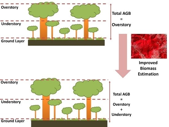
Exploring the Inclusion of Small Regenerating Trees to Improve Above-Ground Forest Biomass Estimation Using Geospatial Data

1
School of Physical, Environmental and Mathematical Sciences, University of New South Wales, Canberra, ACT BC 2610, Australia
2
Institute of Geography, Vietnam Academy of Science and Technology, Hanoi 100000, Vietnam
3
Graduate University of Science and Technology, Vietnam Academy of Science and Technology, Hanoi 100000, Vietnam
4
School of Science, RMIT University, Melbourne, VIC 3001, Australia
*
Author to whom correspondence should be addressed.
Remote Sens. 2018, 10(9), 1446; https://doi.org/10.3390/rs10091446
Submission received: 21 June 2018 / Revised: 3 September 2018 / Accepted: 6 September 2018 / Published: 10 September 2018
(This article belongs to the Section Forest Remote Sensing)

Abstract

:
Research on the contribution of understory components to the total above ground biomass (AGB) has to date received very little attention because most prior biomass estimation studies have ignored small regenerating trees beneath the main canopy with the assumption that their contribution to biomass is generally negligible. Only a few biomass studies have emphasized a considerable contribution to biomass of understory components in forest ecosystems. However, this study of native, tropical, deciduous forest biomass in the Central Highlands of Vietnam was able to explore the contribution of small regenerating trees to total biomass by exploiting a large field inventory of hundreds to thousands of individually-counted small regenerating trees per hectare. Thus, this study investigated the influence of small regenerating tree biomass on models of the relationship between total AGB and remote sensing data. These analyses were trained with and without topographic variables derived from ASTER-GDEM. Our results demonstrate that the inclusion of small regenerating understory trees (R2 = 0.42, NRMSE or %RMSE = 30.5%) provides a quantifiable improvement in total estimated AGB compared to using only large woody canopy trees (R2 = 0.21, NRMSE or %RMSE = 36.6%) when correlating field-based biomass measurements with optical image-derived variables. All analyses show that the inclusion of terrain factors made an important contribution to biomass modeling. This study suggests that for young, open forests where there are many small regenerating trees, the contribution of understory biomass should be taken into consideration to improve total AGB estimation.

Graphical Abstract

1. Introduction

Forests play a vital role in the global carbon cycle since their key indicator, known as biomass, contributes significantly to the mitigation of greenhouse gas emissions through carbon sequestration and storage [1]. Although there are various methods of above ground biomass (AGB) estimation available, ranging from ground-based inventory [2,3] to remote sensing [4,5] and GIS-based techniques [6,7,8], the accuracy of these approaches remains uncertain [9,10]. Improving the accuracy of AGB estimation is important for developing a better understanding of forest ecosystems, and protecting them [11].
Although overstory biomass makes a major contribution to total AGB in multi-layered forests, understory vegetation might add a considerable amount of biomass at some sites, especially in places where there are many young stands of trees [12]. It has been reported that the subcanopy layer comprised 27% of total AGB in a multi-layered Mediterranean forest [13] and an average of 6.8% of total ecosystem AGB in temperate Pinus pinaster Ait. forests in southwestern France [14]. Stand age is an important determinant of the contribution of understory biomass to total ecosystem biomass. In New Brunswick forests, understory biomass was reported to contribute as much as 71–88% of total biomass in 13- and 16-year-old jack pine stands, but as little as 1–6% of total biomass in older stands [12].
Young forests dominated by numerous small regenerating understory trees are common in many forested areas in Vietnam. At the national scale, forests in Vietnam have been in transition since the early 1990s, after decades of deforestation [15]. Although total forest cover has increased since that time, a high rate of deforestation and forest degradation has continued, mainly in the North Central, Northeast, Central Highlands, and Northwest regions [16]. Therefore, most forests include secondary growth or regrowth over large areas. For instance, one study in Yokdon National Park in the Central Highlands has reported a very large number of small regenerating trees mixed amongst older woody stands [17]. It reported that the density was 590 ± 178 individuals per hectare for trees with DBH ≥10 cm, 1229 ± 523 individuals per hectare for trees with DBH ≥1 cm, and 13,383 individuals per hectare in the seedling size class. In addition to a high density of regenerating trees, the Yokdon study reported an extremely high frequency of total trees with a height <6 m compared with those with a height ≥6 m.
During 2013–2014, a forest inventory field campaign was undertaken in Northern Daklak province in the Central Highlands of Vietnam. In this field campaign, many small woody regenerating trees were observed. It raised a question of whether this large number of trees within the understory layers would substantially affect the total AGB of the area. Although understory vegetation comprises many plant types such as grass, herbaceous species, and woody shrubs, together with seedlings and saplings of canopy trees [18,19], this investigation only focused on small, regenerating, woody shrub-like plants. The reason for that selection was because those plants are regenerating saplings of deciduous older woody stands; moreover, the study site includes a very large number of these sapling trees. Therefore, their biomass was considered likely to have a greater impact upon total AGB than other undergrowth species such as grasses and herbs. Their growth rates are also less likely to vary between seasons compared to other understory vegetative life forms.
In general, biomass studies are highly biased in their focus on overstory trees while ignoring understory tree layers [13,20,21,22] due to: the lack of information about underlying vegetation strata [18,23]; the complexity and diversity of understory species [13,24]; an assumption of a negative association between numerous small regenerating trees and total AGB [25,26]; and, the lack of analytical methods for, and difficulty of, calculating the contribution of sub-strata to AGB [27]. Because these underbrush strata are often composed of various-sized, varied-age heterogeneous patches and ordered in a range of vertical layers, measuring field data is either restricted in terms of accuracy or the sample is not fully representative of the whole range of understory communities at the site [28]. Hence, methods of quantifying understory biomass still contain much uncertainty. To date, little research has been carried out to measure the contribution of understory vegetation to AGB [14,29].
There are two common approaches to quantifying the biomass contained in understory vegetation, namely the direct approach and the indirect approach. The direct approach is a destructive method that harvests and weighs dry plant components to develop allometric equations to estimate biomass, which is similar to the approach applied for overstory trees. These allometric equations can be based upon either the biophysical parameters of a single plant or the average of whole species or particular functional groups [18,30,31,32]. However, this approach is both labor-intensive and time consuming [33,34]. Another approach is the indirect and non-destructive method, which characterizes biomass in understory vegetation by using the relationship between understory vegetation and canopy trees [32]. Joyce et al. [28] measured the quantitative relationships between foliar cover and biomass and suggested that this cover/biomass relationship is steady at each site, therefore, biomass can be predicted using only foliar cover measurements. Percentage cover is also commonly used when quantifying understory biomass for many species [32,33,34], and it has been suggested that the combination of percentage cover and height is also useful [32]. However, the practical utility of such models is limited because height is not easily measured in large-scale surveys [32]. In our study, we used allometric equations that employed the maximum dominant height of shrubs to estimate biomass for small regenerating trees in the understory. This understory biomass was then combined with overstory large woody tree biomass to be used as a measure of in situ AGB.
Selection of a suitable allometric equation is an important step in estimating AGB [2,35]. Allometric equations have been developed for different spatial domains, and it has been argued that using region-specific allometric equations produces better results than using a generalized global allometric equation [36]. Application of allometric equations is often highly uncertain and site dependent [37]; therefore, we used regional- and species-based allometric equations pertinent to our particular study area rather than commonly used, generic allometric equations so that our estimations of biomass might concur as closely as possible with available field-based biomass measurements.
Many studies have pointed out that the accuracy of biomass estimation could be improved considerably if the predictor variables included environment-related factors such as topography and climate [38,39]. These studies have indicated that apart from the most important role of remote sensing-derived variables in estimating biomass, these other biophysical phenomena play a crucial role in the performance of biomass models [40,41]; therefore, a good model should include the biophysical factors that strongly influence biomass density. Thus, we investigated two scenarios in this study to test this contention, and therefore compared the results of a model without topographic factors and the results of a model that included topographic factors.
Overall, this study: (i) investigated the effect of including small regenerating tree biomass on improving the accuracy of total AGB estimation; (ii) evaluated the uncertainties of region- and species-specific allometric equations and other generic allometric equations; and (iii) examined the influence of topographic factors on AGB estimation. These analyses were trained with variables derived from Landsat-8 OLI data using both parametric and non-parametric approaches for comparison.

2. Study Area and Data Used

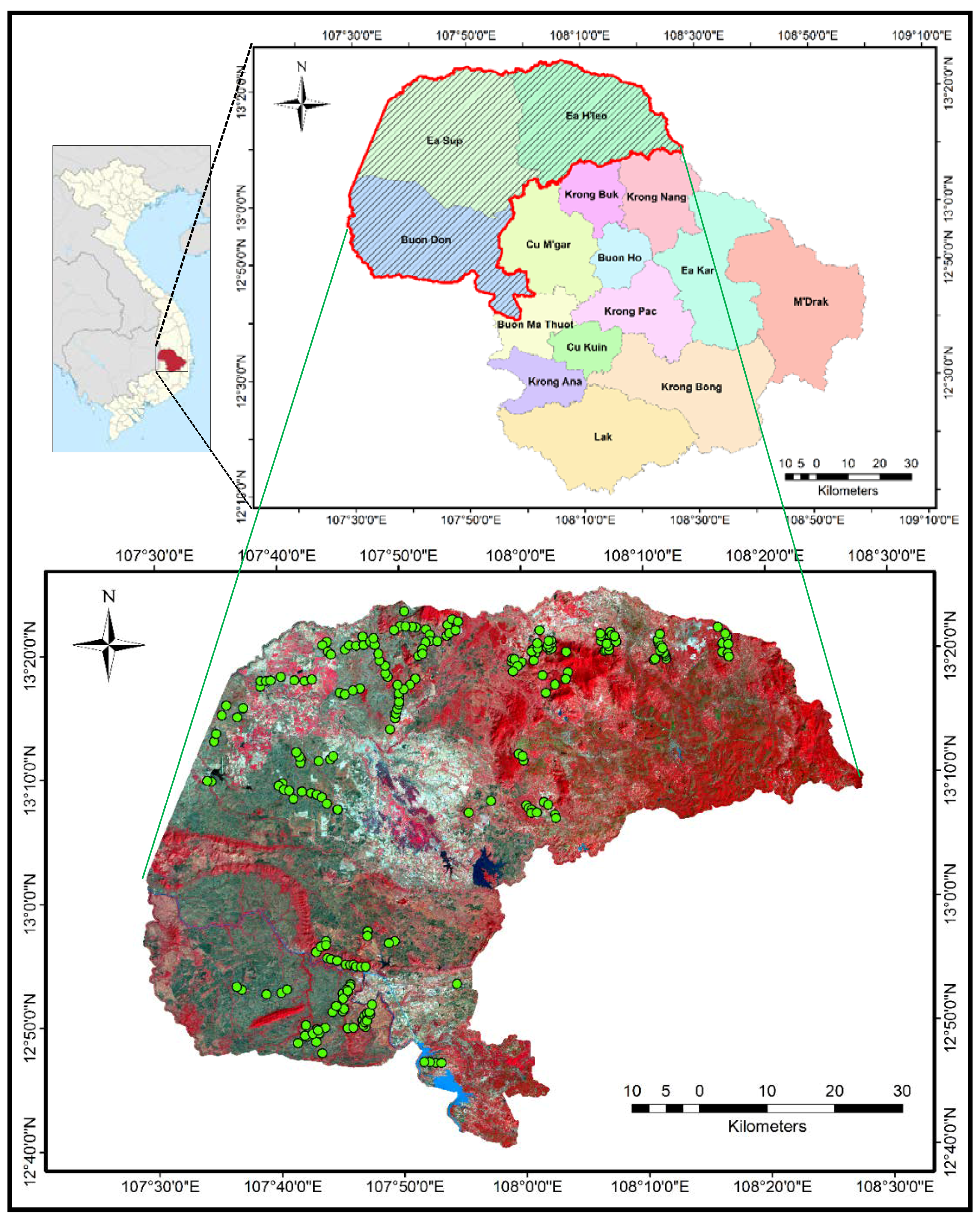
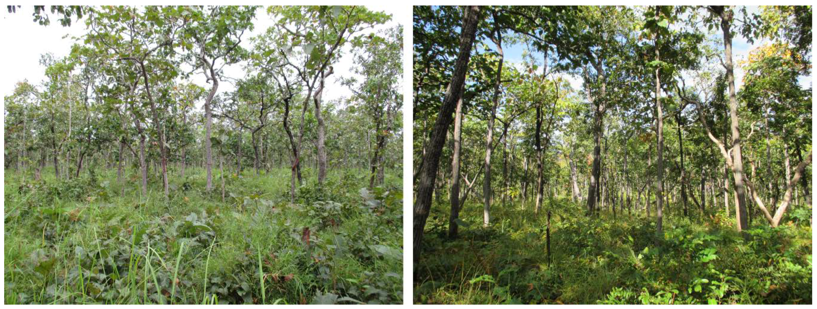
2.1. Site Description

The test site was situated in Northern Daklak province in the Central Highlands of Vietnam, between 12°40′0′′N to 13°25′20′′N latitude and 107°29′0′′E to 108°27′53′′E longitude, and covering an area of about 451,740 ha (Figure 1). The mean elevation ranges from 600–700 m above sea level, with medium undulating slopes having gradients varying from 0° to 58.4°. This area exists in the tropical zone and has two distinct seasons: rainy and dry. The rainy season extends from May to the end of October and contributes around 90% of annual rainfall while the dry season runs from November to April of the following year with little precipitation. Mean annual precipitation ranges from 2200 mm to 2400 mm.
Forests in this area are species-rich and structurally diverse. Not only do they serve an important protective function for soils but they also contain many significant species that have both economic and scientific value; thus, these forests underpin the progress of socio-economic development of the province.
This study focuses on estimating biomass in deciduous dipterocarp forest (DDF), which dominates ~43% of the total natural landcover of the test site. Multiple development stages of regenerating forests have gradually replaced the intact forests of the area, which accounts for the considerable number of small regenerating trees observed there.
Besides shedding leaves in the dry season, these DDFs are characterized by great structural and floristic heterogeneity, and phenological variations due to changes in seasonal and longer-term effects. Dipterocarpus obtusifolius, Dipterocarpus tuberculatus, Irvingia malayana, Shorea obtusa, Shorea siamensis, Terminalia alata and Xylia xylocarpa, are the major tree species. Of those species, Dipterocarpus tuberculatus has been found to be the most numerous within the study area, constituting about one-third of all measured trees. Vegetation distribution and characterization also varies due to complex terrain conditions.
The DDF is the predominant forest type in mainland Southeast Asia [42], extending from Myanmar to Vietnam and parts of India [43]. Across Southeast Asia, the DDFs have been seriously degraded [42] due to natural threats and the impacts of human activities [44,45]. DDFs are understudied [42,46], perhaps because of their complex structure and distribution in addition to their considerable transformation in recent decades [17,44]. In Vietnam, DDFs occupy nearly 650,000 ha primarily within two main ecological regions: the Central Highlands and the South East [47]. Due to their characteristic open canopies, DDFs usually feature a variety of understory subcanopy species.

2.2. Field Data Collection

This study used a total of 226 sample plots that were collected by the National Forest Inventory and Investigation Project campaign (Figure 1). Fieldwork was conducted during the dry season from November 2013 to April 2014, with plots and sub-plots designed to investigate large woody trees and small regenerating trees, respectively.
For large woody trees, which possessed a diameter at breast height of greater than 6 cm (DBH, measured at 1.3 m height above the ground), 1000 m2 rectangular (33.3 m × 30 m) sample plots were set up. Areas were selected to have relatively homogeneous ecological characteristics, such as being of the same deciduous forest type, uniform terrain, and geomorphology, based on the results of preliminary forest inventory mapping from remote sensing image classification along with ancillary maps and the knowledge of forest experts [48].
Although the main focus of this field campaign was forest inventory and investigation, one of the datasets it produced had sufficient accuracy and representativeness to be used to study biomass. In the field campaign, each plot was initially sampled from within a larger homogeneous forest patch identified using SPOT 5 and SPOT 6 image segmentation and the most recent 1:10,000 forest map available. In the field, the geographic location of each plot was adjusted within a radius of 100 m, when required, to ensure it was contained completely within an area of the labeled vegetation type and distant with borders of other vegetation types by at least 50 m. Plots were also removed in those areas found to have mixed forest types. All those adjustments, especially the coordinates of new plot centers, were updated in the field survey sheets.
It is widely known that errors tend to increase when plot sizes are not rational [49,50,51,52]. However, it has been claimed that this relationship holds mainly in forest areas with high variability in forest types [53]. Many biomass studies have used sample plot sizes that were similar to, or not much larger than, comparative remote sensing pixel resolutions; for example, 20 m × 20 m ground plots compared to Landsat 30 m pixels in Uganda [54]; 0.25–5 ha plots compared to MODIS 1 km pixels and QuickSCAT 2.25 km pixels in the Amazon basin [55]; 25.82 m × 25.82 m plots compared to Landsat 30 m pixels and PALSAR 25 m pixels in Northern Guangdong, China [56]; and 0.07–0.1 ha plots compared to Landsat 30 m pixels in Brazil and Bolivia [57].
The sample plots in this study satisfied the criterion of representing a homogeneous forest type (i.e., only DDF). The plots varied only in terms of forest structure, for example by having different vertical dimensions. In other words, the trees measured in this study differed according to size and age, which is not really a spatial problem related to the compatibility of plot sizes and pixel sizes.
At each sample plot, basic biophysical parameters were recorded, including the name and quantity of each tree species, forest type, tree density, DBH, GPS coordinates of the plot center (using a handheld GPS with an accuracy of less than 10 m), site slope, and field photos of individual large woody trees (Figure 2). During the field measurements, trees with a DBH <6 cm were not individually measured but were recorded via counts of small regenerating trees, as described below. The very high diversity of tree species in the natural tropical forest prevented local expert botanists from identifying some individual trees. This had effects upon the determination of wood density, which is a parameter applied to some allometric equations to produce indirect estimates of in situ biomass, which is discussed below. There were 141 plots located in areas with gentle slopes of <10°, 79 plots on moderately steep slopes between 10–25°, and 6 plots on steep slopes of >25°.
Tree height is one of the most important forest structure components when evaluating tree biomass or volume, but accurate measurement of this variable is relatively time-consuming and costly [58]. Although the inclusion of tree height will reduce uncertainty when using allometric equations for biomass estimation, tree height has often been disregarded because accurately measuring the height of each individual is so challenging, especially in closed-canopy forests [59]. Therefore, a common forest inventory procedure is to measure heights of only some representative trees and then estimate the remaining, unmeasured trees’ heights based on the correlation between height and diameter (i.e., H:D relationship), which reduces data acquisition costs [58]. In this field campaign, tree heights were measured for a reasonably large subset of trees (roughly every fifth tree) in each sample plot. Tree height was measured as the vertical distance from the ground to the topmost live leaves using alternatives of Blume–Leiss, Suunto, and Vertex hypsometer instruments and tape. In this study, for trees that had no height measured in the field, a site-specific H:D model was used to predict tree height from diameter. Details about the H:D model’s development can be found in the field campaign’s technical documents [48,60].
As mentioned above, although saplings with a DBH <6 cm were not included in the detailed field measurements, they were recorded via counts of small regenerating trees. In each sample plot, four corner sub-plots of 5 m × 5 m were established to record species names and count the number of individual small regenerating trees in three height classes: <1 m, 1–3 m, and 3–6 m (Table 1 and Figure 3).
For the analysis presented in this paper, the total observed live AGB was calculated as the sum of the biomass of large woody trees plus small regenerating trees. Finally, the AGB of a plot was converted to Megagrams per hectare.

2.3. Remote Sensing and Ancillary Data

Landsat-8 OLI is the latest generation of Landsat sensor, with some enhancement in spectral bands, radiometric resolution (12 bits), and signal to noise performance, when compared to prior Landsat series sensors, which is advantageous for many applications, including vegetation characterization [61]. It is also thought to be an important potential data source for forest management systems, particularly when there is limited capacity to access high-cost, advanced, remotely-sensed LIDAR or SAR data.
In an attempt to extend the research reported here to other forest monitoring missions in Vietnam, and based on current national systems and capabilities, Landsat-8 OLI optical data were selected for this research since they can be freely downloaded and combined with other Landsat generations to undertake temporal forest monitoring. The data were readily obtained from the USGS Earth Resources Observation and Science (EROS) Centre archive (http://earthexplorer.usgs.gov/).
The entire spatial extent of the test site used in this study was covered by just one Landsat-8 OLI scene (path/row 124/51). The spatial resolution of non-thermal bands is 30 m and the data were acquired on 30 January 2014, contemporaneous with the field campaign’s dates. The scene was delivered at processing level L1T Standard Terrain Correction, and was obtained in clear, cloud-free atmospheric conditions. In addition, a free Advanced Spaceborne Thermal Emission and Reflection Radiometer (ASTER) Global Digital Elevation Model (GDEM) with 30 m spatial resolution was downloaded and used to derive terrain variables for biomass modeling.

3. Methodology

The methodology of this study included four main procedures, which are ordered in the following structure: (1) calculating in situ AGB using field measurements and available allometric equations (Section 3.1); (2) pre-processing optical imagery (Section 3.2); (3) deriving variables from the optical image (Section 3.2); and (4) developing models for AGB prediction from the observed plot-based (in situ) biomass measurements and image-derived variables (Section 3.3 and Section 3.4).
Several image-based variables, such as raw spectral bands, band ratios, Vegetation Indices, Principal Components, and texture, were extracted from the image to test their potential for application in AGB estimation. To assess the role of biophysical factors in the models, topographic variables were added to the AGB models. All input variables were trained using two parametric approaches and two non-parametric approaches. The following subsections provide the details for each step of the experiment.

3.1. In Situ AGB Estimation

In situ AGB was estimated from the field measurements. As mentioned above, allometric equations have been developed at various spatial scales (e.g., global and regional), but it has been argued that using region-specific allometric equations produces better results than using a general, global allometric equation [36]. In this study, we used one region- and species-specific allometric equation developed for our particular study area by UN-REDD (The United Nations Programme on Reducing Emissions from Deforestation and Forest Degradation) [62]. This UN-REDD project developed allometric equations for several frequently occurring species in the Central Highlands area, but here we used only the equation that was applicable to deciduous forests. Additionally, we used other generic allometric equations for closely related eco-regions or forest types to then compare and evaluate their predictions. These equations used either a single input, DBH (Equation (2)), combined DBH with Height (H) (Equation (3)), or combined DBH, H, and Wood Density (WD) (Equations (4) and (5)). We sourced wood densities from the global wood density database [63] based on the field campaign records of trees’ scientific names. However, as noted above, some individual trees could not be identified to the species level, so wood densities could not be determined for those trees. Instead, the arithmetic mean of the wood density of the known tree species in the same plot was computed and assigned to the unknown tree species [2] (in Table 2).
B = 0.14 × DBH2.31
B = exp (−2.134 + 2.53 × ln (DBH))
B = exp (−3.1141 + 0.9719 × ln (DBH2 × H))
B = 0.0673 × (WD × DBH2 × H)0.976
B = exp (−2.409 + 0.9522 × ln (DBH2 × H × WD))
Y = 0.39 + 3.22 × Hmax
In addition to calculating biomass for large woody trees, we computed the biomass of small regenerating trees using equations taken from [23]. We wanted to include the large number of small regenerating trees observed in the field plots in our investigation to determine their contribution to total AGB. Using the formula provided, we used the maximum height of each height class to compute small regenerating tree biomass. Because individual tree heights were not measured for each small regenerating tree, we assigned a representative height value for each group. These heights were: 1 m for the <1 m height class, 3 m for the 1–3 m height class, 6 m for the 3–6 m height class.
We calculated the biomass in kilograms of each large woody tree and each height class of small regenerating trees, and then summed the biomass of each plot and converted it to Megagrams per hectare (Mg/ha).

3.2. Remotely Sensed Data Pre-Processing and Creation of Derived Variables

We used six spectral bands of visible and infrared reflectance (Bands 2–7) from Landsat-8 OLI. This analysis required spectral information to be in the form of top of atmosphere (TOA) reflectance rather than digital numbers (DN), thus, we converted the Landsat-8 OLI scene first to TOA reflectance using the formulas (Equations (S1) and (S2)) provided in the USGS guidelines (https://landsat.usgs.gov/using-usgs-landsat-8-product).
We then geometrically corrected the scene using the WGS84 datum, projected it into UTM Zone 48 N using image registration with the ground control points (GCPs) taken from a 1:50,000 scale land use map and a 1:50,000 scale administrative map. We used a first-order polynomial function and the nearest-neighbor resampling method, and the resulting error was less than one pixel. Finally, we clipped the optical bands using the administrative boundary vector layer. Similar to several other studies [54,65,66], we did not apply atmospheric correction in this experiment for three reasons: (1) all sample plots were located within only one Landsat scene so it can be assumed that atmospheric conditions were homogeneous for all plot locations; (2) absolute atmosphere-corrected reflectance values are not necessarily required for this kind of empirical method; and (3) more uncertainty may be generated through an atmospheric correction step if atmospheric information is not available for the site.
After pre-processing the Landsat-8 OLI scene, we derived five different types of variables (Table 3) to construct the AGB estimation model: (1) raw spectral band reflectance; (2) Vegetation Indices; (3) spectral band ratios; (4) Principal Component bands; and (5) texture. All optical imagery-derived variables are listed in Table 3.
We selected the spectrally-derived variables based on their predictive capacities for AGB estimation and their past successful application in previous studies [4,40,41,74,75,76,77]. We completed all processing of these Landsat-derived variables using ENVI 5.3 software.
Window size plays an important role in texture performance [77]. A window size that is too small may misrepresent pixel brightness variations but retain high spatial resolution, while a window size that is too large may skip important information about image tone variations due to over-smoothing the textural variations [77,78]. However, no particular window size has been suggested as the best option for all texture approaches in biomass studies. Generally speaking, most studies have implemented a range of window sizes then selected the final optimal window size based on a comparison of obtained results [77] and these sizes vary depending upon the criteria of texture measurement, the spatial resolution of the dataset, and the density and structure of the forest in that study area.
In the present study, we calculated texture measures using five window sizes, from small to medium sizes, including: 3 × 3, 5 × 5, 7 × 7, 9 × 9 and 11 × 11 pixels. We then determined the final optimal window size after comparing the outputs. Considering the results of correlation coefficients between texture parameters obtained from testing different window sizes and in situ biomass, along with the pixel size of Landsat data, a final window size of 3 × 3 was selected for the experiments (Table S1). This is in line with a number of other studies, which also ended up choosing a 3 × 3 window size for their final biomass estimation models after testing a range of window sizes [54,61,77].
To estimate AGB, other factors relating to topography, climate, and environment have been taken into consideration in biomass models [39,40,41,77]. In our study, we focused only on topographic variables to assess their influence in biomass prediction. Three main topographic variables, namely elevation, slope, and aspect, were included in the models. These variables were computed from the ASTER GDEM 30 m, using ArcGIS 10.1.

3.3. Regression Algorithms

As mentioned above, we investigated both parametric and non-parametric approaches to test their potential for AGB estimation. For each regression approach, we selected two methods for conducting experiments. Our selection was based on their prior successful use in previous studies [79]. The two parametric methods were Multiple Linear Regression (MLR) and Stepwise Multiple Linear Regression (SMLR), while the two non-parametric methods were Random Forest (RF) and Support Vector Machine (SVM). We compared the results obtained from each method with the others to identify the best-fit model for AGB estimation. A brief introduction to these methods follows.
MLR is a parametric regression approach that models the relationship between two or more predictor variables and a dependent variable. This approach requires an assumption of a linear relationship between independent variables and a dependent variable, but the correlation between predictor variables should not be too high, so that they may be considered to be independent to avoid multicollinearity. Multicollinearity can cause regression coefficients to become very sensitive to small changes in the model or may reduce the accuracy of the estimated coefficients. Normally distributed residuals are also required in MLR. The final MLR assumption is homoscedasticity, which states that the variance of error terms is similar across values of the independent variables. MLR is quite sensitive with regard to outliers. When the number of predictor variables is large, there is a high likelihood MLR is faced with multicollinearity and overfitting problems, thus parsimonious independent variable selection is important [80].
SMLR is another robust, parametric approach that can help to find the optimal independent variables for the model. Depending on the stepwise selection method used, either backward or forward, predictor variables are either subtracted or added at each iteration. However, similar to other parametric methods, SMLR still requires a linear relationship between predictor variables and the dependent variable. In addition, a high likelihood of multicollinearity and overfitting issues remain when many predictor variables are included [66]. SMLR also has problems with producing high bias R2. Because SMLR adds or removes variables in a particular order, it might underestimate the combinations of variables. This may lead to misinterpretation of the data. Moreover, the final model selected from SMLR may suffer from overfitting due to sample variances. It is noted that outliers should be eliminated before employing the method. Sample size also has a great impact as it is suggested that the more variables that are available, the more observations need to be used. Although SMLR is not recommended for testing hypotheses, using SMLR is useful in investigating the significance of variables for the model [81].
RF is an ensemble learning method performed by constructing an interconnection of a large set of decision trees at training time and outputting the mean of each prediction, using a subset of random samples and different initial variables [82]. RF is a non-parametric method that has been widely used in biomass modeling, with the advantages of being able to process numerous input variables and overcoming the overfitting problem. Variables do not need to satisfy any particular statistical distributional assumption in the RF model.
SVM is another promising non-parametric alternative that is also a supervised machine learning approach. The basic concept of this method is that of transforming the inputs into a higher-dimension feature space using a kernel function [79]. This transformation changes the relationship from a nonlinear to linear one in the new feature space. For this method, careful choice of regression parameters plays a key role in model performance [83]. As with other non-parametric approaches, SVM minimizes the overfitting problem.
Our models were trained using observed, plot-based biomass and the corresponding values of raw spectral band reflectances, spectral band ratios, Vegetation Indices, Principal Components, and texture for plot locations. We implemented all four statistical algorithms for developing AGB prediction models in the open source R software using a variety of packages: MLR and SMLR using the “MASS” package [84], RF using the “randomForest” package [85], and SVM using the “e1071” package [86].

3.4. Modeling Approaches

For further analysis, we computed mean values for the derived image variables based on the corresponding geographic location of sample plots. To be able to make a good choice of variables, we tested the Pearson’s r correlation between individual predictor variables and in situ AGB. We then selected variables that had high correlations.
r = ( x i x ¯ ) ( y i y ¯ ) ( x i x ¯ ) 2 ( y i y ¯ ) 2
where x is the observed value, x ¯ is the mean of the observed values, y is the predicted value, and y ¯ is the mean of the predicted values.
We used these final variables to build the AGB models. To achieve the proposed objectives, we trained all the variables derived from Landsat-8 OLI and the ASTER GDEM in six different tests as follows:
  • Test 1: Test 11 (Raw spectral bands) versus Test 12 (Raw spectral bands + topographic variables)
  • Test 2: Test 21 (Vegetation Indices) versus Test 22 (Vegetation Indices + topographic variables)
  • Test 3: Test 31 (Raw spectral band ratios) versus Test 32 (Raw spectral band ratios + topographic variables)
  • Test 4: Test 41 (PC bands) versus Test 42 (PC bands + topographic variables)
  • Test 5: Test 51 (Texture) versus Test 52 (Texture + topographic variables)
  • Test 6: Test 61 (All Landsat-derived variables combined) versus Test 62 (All Landsat-derived variables combined + topographic variables)
The purpose of this test group division was to determine the optimal set of variables. In each test group, two scenarios were investigated using the same set of image-derived variables, with the only difference being the inclusion of topographic variables. We designed these scenarios to evaluate the involvement of topographic factors in biomass prediction.
Some outliers were removed from the samples to reduce uncertainties. We identified outliers using a histogram and boxplot approach. Approximately 3% of sample plots were deemed to be outliers and thus removed.
Validation of the biomass estimation models was an important step to assess whether the AGB model we developed could perform well in practice. Ideally, this step should be based on a new set of sample plots, but in most studies, including ours, this approach is routinely neglected due to the impracticality or infeasibility of conducting further field data collection. Therefore, whole sample sets are usually divided into two subsets: one subset for model training and the remaining subset for model validation. In some cases, if the number of sample plots is limited, cross-validation can be applied. In the present study, considering the number of sample plots and the large number of variables used, we used ten-fold cross-validation for model building and testing. In other words, we randomly split the field-sampled forest AGB dataset into ten folds and then each fold was sequentially used as a validation subset while all remaining data were used for training purposes. We repeated this process ten times and the final accuracy assessment was computed from the mean error of each run.
We carried out the validation steps using an R script. We computed three common statistical parameters, the coefficient of determination (R2), Root Mean Square Error (RMSE), and Normalized Root Mean Square Error (NRMSE) that results in a percentage (%RMSE), to assess and compare the regression models’ performance. A model with a good fit has a low RMSE, low NRMSE and high R2 because a low RMSE and NRMSE indicate high accuracy while a high R2 expresses how well the observed AGB is predicted by the model. These statistical parameters were computed as follows:
R 2 = ( y i ^ y ¯ ) 2 ( y i y ¯ ) 2
where yi is the observed value, y i ¯ is its mean, and y i ^ is the fitted value.
RMSE = 1 n i = 1 n ( y i y ^ i ) 2
where n is the number of observed values, yi is the observed value, and y i ^ is the estimated value.
NRMSE = 1 n i = 1 n ( y i y ^ i ) y ¯ × 100
where n is the number of observed values, yi is the observed value, y i ¯   is   its   mean ,   and   y i ^ is the estimated value.

4. Results

4.1. In Situ AGB Estimation from the Forest Inventory

Table 4 shows the results of biomass calculations from field data measurements using different allometric equations. The plot-based total AGB values ranged from 5.37 Mg/ha to 210.31 Mg/ha using the UN-REDD equation. We observed large variation in large woody tree-based AGB when we applied different allometric equations, which is in agreement with other studies [37]. In the present study, we paid particular attention to the AGB computed from the equation developed by UN-REDD.
The biomass of small regenerating trees among the sample plots ranged from 1.08 Mg/ha to 233.01 Mg/ha. The plot with the greatest biomass of small regenerating trees included 49,000 trees < 1 m, 4800 trees in the 1–3 m height class, and 400 trees that were 3–6 m in height.
Our results (Figure 4) show the biomass of large woody trees (bars in orange color) and the biomass of small regenerating trees (bars in blue color) in each plot. The figure suggests that no clear relationship of large woody tree biomass and small regenerating woody tree biomass exists because high variability of small regenerating woody tree biomass occurs regardless of the amount of large woody tree biomass present at the plots.
Consequently, the variation between biomass estimates before and after adding small regenerating trees is quite high (Table 5). In this study area, large woody tree biomass was mainly in the range of low biomass (from 0–100 Mg/ha). However, the inclusion of small regenerating tree biomass dramatically increased the value of the total AGB in each sample plot, which increased the percentage of plots in higher biomass classes (100–150 Mg/ha, 150–200 Mg/ha, and >200 Mg/ha) irrespective of which equation we used. This highlights the significant contribution of small regenerating trees to the total biomass of the plots [14,87].

4.2. AGB Estimation from Satellite Data

Figure 5 and Figure 6 compare the R2 and NRMSE (resulting from the RF algorithm) for the total AGB estimates from different allometric equations including large woody trees and small regenerating trees. In both analyses, results from allometric Equation (1) [62] provided the highest R2 (Figure 5a,b) and the lowest NRMSE (Figure 6a,b) compared with other allometric equations. Generic Equation (2) [64], which uses only the DBH parameter, produced the highest uncertainty, with the lowest R2 and the highest NRMSE. The two equations, Equations (4) and (5), using the same parameters of DBH, H, and WD provided comparable results. When comparing generic Equation (3), which used DBH and H, with Equations (4) and (5), which included DBH, H, and WD parameters, the equation without WD produced higher certainty. As mentioned previously, the species name of a number of individual trees could not be identified by local botanical experts, so the replacement of the specific WD value with the mean WD value of known trees in the plots might have introduced some uncertainty.
When comparing the coefficient of determination (R2) between total AGB (i.e., large woody + small regenerating trees) versus large woody tree biomass alone in Figure 5a,b, it is clear that the total biomass is better explained by the models than biomass of large woody trees alone. Similarly, the comparison of NRMSE (%RMSE) in Figure 6 demonstrates the better performance of total AGB, which includes small regenerating trees, rather than a model with only large woody tree biomass.

4.3. Assessment of Optical Imagery-Derived Variables

To identify which Landsat-derived variables were most important in building the AGB models, we computed correlation coefficients between field-based biomass and each group of predictor variables (Table S2). The size of the correlation coefficient varied slightly between different equations for all variables, but the direction of the correlation between the predictors and biomass was consistent. In brief, all raw spectral bands’ reflectance had a strong correlation with field-based biomass except bands 2 (Blue), 4 (Red) and 7 (SWIR-2), which had a very strong relationship with biomass compared to the other bands. However, because all spectral bands had a strong correlation with biomass, we used the reflectance of all spectral bands in further experiments. We did not use the BLUE/GREEN ratio to build biomass prediction models due to its weak correlation with field-based biomass across all of the allometric equations. Similarly, in the group of VIs, we did not use GEMI in the models because of its weak correlation with biomass. In terms of Principal Components, the second PC had the strongest association with biomass, albeit it was a negative relationship, while the third PC was eliminated in the biomass prediction due to its weak correlation. Biomass had a positive correlation with the first PC. Analysis of correlation coefficients between texture variables and field-based biomass showed that the mean texture parameter (ME) had the strongest correlation, while other texture parameters had quite weak correlations with biomass and were not significant [8]. Therefore, only ME was used in building the biomass models in this experiment. The abovementioned strongly correlated variables selected from each variable group test were used in the Test 6 experiment.
The findings in Table 6 and Table 7 indicate that in all four types of regression algorithms, the use of raw spectral band variables (Test 1) and all variables combined (Test 6) yielded a better AGB prediction, with a higher R2 and lower RMSE than other tests. Band ratio variables (Test 3) and texture variables (Test 5) provided comparable AGB estimates. Comparatively, AGB estimates derived from VI variables (Test 2) and Principal Component variables (Test 5) were weaker than the results from other variable groups. Other studies have demonstrated that VIs are not robustly and significantly related to forest biomass [4,61], although these relationships are quite inconsistent.

4.4. Performance of Topographic Variables

Of the topographic variables, aspect had the lowest correlation with biomass while elevation and slope each had a similar relationship to biomass. Elevation had the highest correlation with biomass across all equations (Table 8).
Although the difference between the results of the two scenarios is generally not distinctive, Table 6 and Table 7 also demonstrate that all experiments that included topographic variables performed better than the experiments excluding topographic variables. This difference was highlighted strongly in the RF algorithm, with the R2 value rising from 0.39 to 0.48 in Test 1, from 0.39 to 0.47 in Test 3, and from 0.38 to 0.46 in Test 6.

4.5. Performance of Regression Methods

The results revealed that the most robust predictor variables differed slightly between regression algorithms (Table 6 and Table 7). In general, the groups of raw spectral bands (Test 1) and all optical imagery-derived variables combined (Test 6) provided superior results for all regression methods. Comparatively, the biomass estimate can be explained relatively well from texture (Test 5) in ML, SML and SVM. It is noteworthy that band ratios (Test 3) played a similar role in biomass prediction using MLR and RF methods, but performed more poorly in the two remaining regression methods, SMLR and SVM.
Comparing different regression algorithms, the RF method was the best among the four methods while results of all tests using RF produced less uncertainty than other methods (Figure 7). For example, the RF tests revealed the most powerful predictors to be the raw spectral band variables in Test 1 (Figure 7a), which produced an R2 of 0.48 and RMSE of 46.22. Band ratio variables in Test 3 (Figure 7c) resulted in an R2 of 0.47 and RMSE of 46.42. The combined variables in Test 6 (Figure 7f) yielded an R2 of 0.46 and RMSE of 46.49. The SVM method produced R2 and RMSE values that were not much different to the other methods, however, it performed remarkably well compared to the other methods in the Texture test group (Figure 7e), with an R2 of 0.42 and RMSE of 48.66. In summary, our results demonstrated that non-parametric methods performed better than parametric methods for estimating AGB.

5. Discussion

5.1. In Situ AGB Estimation from the Forest Inventory

In this experiment, it is difficult to estimate the absolute biomass value of the small regenerating trees because the DBH and exact height were not measured for every individual tree. As we used the maximum height (Hmax) of a class in the formula, our approach overestimates the biomass of the small regenerating trees compared to the actual biomass.
It seems likely that sample plots with high biomass derived from large woody trees would have low biomass derived from small regenerating trees and vice versa. This is understandable because when the plot’s area is mainly occupied by large woody trees, there is neither much room left for small regenerating trees nor much light reaching the ground because of competition from the large woody trees. On the other hand, disturbed forest plots with fewer large woody trees might be much more likely to be dominated by small regenerating trees.
Overall, the result highlights the importance of using site-specific allometric equations in biomass studies as they consistently provide higher accuracy and lower uncertainty than generic equations.

5.2. AGB Estimation from the Satellite Data

Landsat-derived variables provide better biomass estimates for total AGB than they do for large woody tree biomass alone. This means that small regenerating tree biomass should be included in total AGB estimation to get a better-fitting relationship between biomass and Landsat remote sensing data.
This finding makes a significant contribution to our understanding of open forests that have similar disturbance histories to those included in this study. The DDF forests of Vietnam, in particular, and Southeast Asia, in general, have become seriously degraded and deforested over the last several decades due to a combination of natural threats, forest fires and anthropogenic impacts [17]. However, reforestation efforts have recently become widespread in response to environmental policies such as the Programme on Reducing Emissions from Deforestation and Forest Degradation (REDD+) or Payments for Environmental Services (PES) [88]. Therefore, many areas of DDFs include numerous young trees with low density, open canopies and a substantial understory of small regenerating trees. When estimating biomass of these young forests, it is important to be aware of, and to account for, the impact of small regenerating trees in the understory.

5.3. Assessment of Optical Imagery-Derived Variables

The strength and direction of the relationship between variable groups and AGB was inconsistent among regression techniques and between experiments with and without topographic variables. For example, observation of different regression groups in the model without topographic variables indicated that: in MLR, raw spectral bands, texture, and all combined variables produced the same highest value of R2 = 0.4; in SMLR, the highest value of R2 = 0.41 was obtained from raw spectral bands and texture; in RF, the highest value R2 = 0.39 was observed from raw spectral bands and band ratios; and in SVM, the highest value R2 = 0.41 was taken from the combined variables. On the other hand, the model with topographic variables yielded the highest value R2 of 0.42 for raw spectral bands and texture using MLR, and the highest value of R2 of 0.44 for SMLR using the raw spectral bands.
Kajisa et al. [89] found that spectral bands were better for biomass estimation than texture while Lu et al. [90] suggested that the combination of spectral bands and texture could improve accuracy. Similarly, a study by Vicharnakorn et al. [41] demonstrated that although Landsat spectral bands were highly correlated to AGB, robust biomass prediction was achieved if the model used the combined variables of Landsat bands, VIs, and elevation.
We selected Landsat for this experiment because Landsat has been used in many studies of AGB [29,54,74,75,91,92]. This is due to its freely accessible archive [93], its global coverage, and its long-term record, which is well-suited for time series studies [39,40,94]. On the other hand, the use of other data like SAR, LIDAR or high-resolution optical images typically requires considerable financial investment and access to high performance computing as well as advanced technical skills to process data, which remain challenges for existing forest monitoring systems in many developing countries [41]. These challenges are in addition to the limited availability of those data in terms of spatial coverage and capacity to afford high data costs [76]. Therefore, using optical images, especially freely available data, is currently the most popular and financially manageable solution for developing countries [95], which is the case for forests in Vietnam [96]. In some circumstances, researchers have found that it is possible to use Landsat for biomass measurement with a reliable level of accuracy at national scales [54,57] because Landsat data are sensitive to vegetation structure, the wide swath coverage of each scene is suitable for regional scales, and Landsat’s spatial resolution is compatible with sample plot sizes [54]. In addition, the selection of data for analyzing the transferability of a biomass model from one site to another should be practically feasible in most areas. Hence, Landsat is a data source that could be ideally used for transferability studies [97] if the forest is not too dense. Moreover, the new design of the Landsat 8 OLI sensor promises a number of opportunities for improving forest biomass estimation accuracy [76].
As can be seen in Figure 2, the study area examined in this research is composed of secondary regenerating forests, in which the tree trunks are small and lack many complex branches, the overstory has an open canopy, and the biomass ranges are not particularly high (typically ranging from 50–100 Mg/ha for large woody tree biomass as illustrated in Table 5). It is widely suggested that, with dense forests, microwave data produces superior biomass estimation but, for young forests, optical data has been proven to produce acceptable estimates [54].
Nevertheless, similar to other biomass studies using optical data [38,74], our values for the coefficient of determination were not very high due to the limitations of optical data (generally having an R2 of around 0.4–0.5, which is consistent with results in Tian et al. [98]). The uncertainties in our results could have been potentially introduced by some of the following errors. Firstly, using optical sensors in AGB estimation is known to present challenges due to their limited ability to penetrate through canopy layers. Secondly, if vegetation in a plot is homogeneous in terms of tree size and species, the mean value of AGB in each plot is a good representation, however, our plots often consisted of heterogeneous trees with different deciduous species and sizes. In some cases, a few distinctive, oversized trees in a plot could cause the mean biomass to be dramatically changed. Therefore, the relationship between spectral variables and field-based biomass could be greatly affected. Thirdly, the allometric equations themselves introduce uncertainties into field-based biomass calculations. In this study, due to the use of region- and species-specific allometric equations for large woody trees, the uncertainties might originate from using the equations to calculate the biomass of small regenerating trees. Fourthly, the boundary of the pixel window used to extract spectral variables and field plots might not have completely overlaid both features due to errors from image pre-processing. Fifthly, uncertainties might be due to the common problem of data saturation at high biomass levels, especially with optical data. Lastly, the selection of the most suitable predictor variables and the limitation of empirical regression models remains a challenge. Understanding the sources of uncertainties will necessitate more research to address these problems and reach greater AGB estimation accuracies.
This study is only one part of a series of experiments that evaluated the contribution of small regenerating trees to total AGB using different types of geospatial data. Landsat is only one source in the list of data used in the broader research. Subsequent studies will assess other kinds of data and the integration of optical and SAR data to further assess the impact of the understory layer on total AGB.

5.4. Performance of Topographic Variables

The observation agrees well with other studies, which emphasize the role of topographic variables [40], especially the strength of elevation as a predictor [41].
The strong correlation between topographic variables and biomass can be explained by the fact that each species adapts to particular climatic and environmental conditions. Climatic and environmental conditions vary depending partly due to elevation. Elevation affects temperature, moisture, wind, insolation, growing season length, geology, and human activities [99], which all affect plant development. Additionally, in some contexts, it is supposed that elevation would affect the rate of photosynthesis, with higher elevation resulting in reduced photosynthesis due to lower availability of CO2, drop in air temperature and barometric pressure [100]. Therefore, an elevation increase might lead the mean AGB to decrease due to these climatic and environmental features [101]. On the other hand, other studies have demonstrated a strong positive correlation between mean AGB and elevation [102]. In other words, AGB tends to increase at some levels of higher elevation because many anthropogenic factors and forest fires have lower impacts at these elevations [103]. Whichever the direction of the relationship at a particular location, it is clear that models for estimating biomass should include elevation along with other environmental factors [3,101,104].

5.5. Performance of Regression Methods

Our observations are comparable to previous work by Powell et al. [40] who demonstrated that RF was the most robust model compared with three regression methods and concluded that RF performed best in test sites in Arizona and Minnesota, with the lowest RMSEs of 39.23 and 32.19, respectively. Avitabile et al. [54] found that RF can be used effectively to demonstrate the complex relationship between AGB and spectral data if the training data are characterized for the variation of biomass density.
It is also apparent why parametric regression methods have proved to be less powerful when using several variables: they are highly likely to be multicollinear. Therefore, parametric regression methods are unsuitable to use in this kind of experiment because they are not well suited to take advantage of multiple variables [80]. While the forest in this area has a complex vertical structure, the RF predictors tend to measure the dissimilarity among observations. This could explain its superior performance in the experiment. Additionally, the RF dissimilarity is known as a method that copes well with mixed variable types. This experiment used a large number of variables of different types and value ranges (spectral, VIs, band ratios, PCs, Texture, Topography and combined variables). Hence, RF would be predicted to be a better model in this case. Future studies that integrate optical and SAR data should exploit this characteristic of RF as inputs derived from the combination of optical and SAR imagery are even more various and numerous. On the other hand, single decision trees often contain high variance or high bias. In regression, RF takes the average predictions of all individual trees, trained on different sections of the same training set to reduce the variance. Introducing the right sort of randomness helps RF become an accurate regressor. Moreover, RF has the capability to avoid overfitting, which is a frequent problem encountered when calculating in situ biomass [79]. All of these factors help to explain why RF performed better than other regression methods in this study.
The scatterplots in Figure 7 indicate that biomass tends to saturate at high levels (above ~180–200 Mg/ha). Avitabile et al. [54] found their models were likely to saturate around 150–200 Mg/ha, but this saturation threshold was more clearly identified in the highest biomass sample plots. This saturation issue reduces the accuracy of the biomass estimation models [94].
All of the scatterplots in Figure 7, especially those showing the RF algorithm, clearly indicated a tendency to underestimate at high biomass values and overestimate at lower biomass values. A similar trend has also been observed in many other studies [29,54,75,105]. Although there was no height measurement taken for each small regenerating tree during the field campaign, assuming each small tree is the maximum height in the height class would overestimate the true AGB. Similarly, the H:D allometric equation used for estimating heights of unmeasured large woody trees also introduced some errors. Another source of biomass underestimation for DDF in this study is that both fieldwork and image acquisition occurred during the dry season when some trees may have dropped their leaves. However, only the actual value of biomass is affected by this underestimation. The model performance will not take account of this uncertainty because both in situ biomass and image-estimated biomass are obtained from the data of the same season.
Selection of data obtained in the dry season prevents misclassification between evergreen vegetation species or other non-deciduous species and deciduous species [54]. Additionally, acquiring optical images in the dry season reduces the probability of cloud contamination of the scenes. In the case of this study site, many plots included trees that were younger than 10 years old, noting that the date of the most recent harvesting ranged from 1980 to 2005, and they had low density biomass with ~42% of the plots ranging 0–50 Mg/ha and ~46% 50–100 Mg/ha (Table 5). This reflects the limited level of canopy closure of the woody tree biomass in this study area. In other words, there may have been limited impact on biomass estimation accuracy during a leaf-off stage.
Dry season estimates of biomass have been included in other studies of deciduous forests [106]. Moreover, it is important to employ multi-temporal datasets for further study of seasonal phenological behavior for DDF. However, optical data can present challenges for such time series studies because cloud cover in tropical areas always restricts the number of usable images. Therefore, seasonal studies of phenological effects would benefit by including SAR data for complementary studies. However, SAR data is sensitive to water content, which should be taken into consideration when analyzing images acquired during the rainy season.
Although not all the tests in this experiment provided very high certainty, they nevertheless illustrated the contribution of small regenerating trees to total AGB estimates. This finding demonstrates that the role of small regenerating trees should not be discounted, especially for tropical forests where a number of different tree layers is common.

6. Conclusions

A key finding of this study was the importance of including small regenerating tree biomass in total AGB calculation when their abundance is high in field plots. As this component of biomass is often neglected, biophysical parameters of small regenerating trees are usually not measured in field campaigns. Thus, the benefit to accurate biomass estimation of more detailed measurements of small regenerating trees should be taken into consideration. Through this study, we have illustrated the influence of small regenerating trees on total AGB and furthered our understanding of total AGB. However, this observation might be most important in areas where the open canopy layers are young and there are many small regenerating trees in the understory. The forests that are in transition from deforestation to a new stage of reforestation frequently fit this scenario. This study also highlights the need to develop site-specific allometric equations for both overstory and understory layers to increase the accuracy of biomass models.
We used only Landsat optical data in this study and our results are consistent with other similar studies, which identified limitations of optical data. The next logical step in this research is to integrate SAR and optical data in a similar analysis to determine if uncertainty also decreases with the inclusion of small regenerating tree biomass. An assessment of the contribution of small regenerating tree biomass using only microwave remote sensing data is another experiment that ought to be conducted.
Topographic factors have previously been identified as important variables in biomass prediction models. Our analysis concurs that elevation is a topographic factor that plays a critical role in AGB estimation. Therefore, designers of the location of field sampling plots must pay attention to topography, with site characteristics such as slope, aspect, elevation, and relief being recorded as a matter of course.
Finally, this study demonstrated that the Random Forest (RF) non-parametric method (R2: 0.48, RMSE: 46.22) outperformed parametric methods (R2: 0.42, RMSE: 48.06, for Multiple Linear Regression; R2: 0.42, RMSE: 47.42, for Stepwise Multiple Linear Regression) when comparing field-based biomass measurements with models built from optical image-derived variables. This might have been due to the complicated configuration of tree stands and canopy structure as well as the density of mixed large woody and small regenerating trees in the sample plots. Therefore, non-parametric methods are more suitable in such forests since they do not require particular statistical distributions.

Supplementary Materials

The following are available online at https://www.mdpi.com/2072-4292/10/9/1446/s1, Equation (S1): Formula for calculating TOA planetary reflectance, without correction for solar angle; Equation (S2): Formula for calculating TOA reflectance with a correction for the sun angle; Table S1: Correlation coefficients between GLCM texture parameters (in different window sizes) and in situ biomass (calculated from Equation (1)); Table S2: Correlation coefficients between optical image-derived variables and total field-based biomass (both large woody and small regenerating trees), computed from different allometric equations.

Author Contributions

Conceptualization of the experiments: A.V.L., D.J.P., and A.L.G. Performed the experiments: A.V.L. Data analysis: A.V.L. Wrote the paper: A.V.L., D.J.P., and A.L.G. Supervision: D.J.P. and A.L.G.

Funding

This research received no external funding

Acknowledgments

The authors are highly thankful to the Institute for Forest Ecology & Environment—Vietnam National University of Forestry for access to the field data. This research was conducted as part of a Doctoral thesis, so we would like to thank the University of New South Wales, Australia, for a PhD scholarship and travel support. We also thank anonymous reviewers for insightful comments on the manuscript.

Conflicts of Interest

The authors declare no conflict of interest.

References

  1. Gibbs, H.; Brown, S.; Niles, J.; Foley, J. Monitoring and estimating tropical forest carbon stocks: Making REDD a reality. Environ. Res. Lett. 2007, 2, 045023. [Google Scholar] [CrossRef]
  2. Brown, S.; Gillespie, A.J.; Lugo, A.E. Biomass estimation methods for tropical forests with applications to forest inventory data. For. Sci. 1989, 35, 881–902. [Google Scholar]
  3. Chave, J.; Réjou-Méchain, M.; Búrquez, A.; Chidumayo, E.; Colgan, M.S.; Delitti, W.B.C.; Duque, A.; Eid, T.; Fearnside, P.M.; Goodman, R.C.; et al. Improved allometric models to estimate the aboveground biomass of tropical trees. Glob. Chang. Biol. 2014, 20, 3177–3190. [Google Scholar] [CrossRef] [PubMed]
  4. Foody, G.M.; Cutler, M.E.; McMorrow, J.; Pelz, D.; Tangki, H.; Boyd, D.S.; Douglas, I. Mapping the biomass of Bornean tropical rain forest from remotely sensed data. Glob. Ecol. Biogeogr. 2001, 10, 379–387. [Google Scholar] [CrossRef]
  5. Kasischke, E.S.; Christensen, N.L.; Bourgeauchavez, L.L. Correlating radar backscatter with components of biomass in loblolly-pine forests. IEEE Trans. Geosci. Remote Sens. 1995, 33, 643–659. [Google Scholar] [CrossRef]
  6. Brown, S.; Gaston, G. Use of forest inventories and geographic information systems to estimate biomass density of tropical forests: Application to tropical Africa. Environ. Monit. Assess. 1995, 38, 157–168. [Google Scholar] [CrossRef] [PubMed]
  7. Brown, S.; Iverson, L.R.; Lugo, A.E. Land-use and biomass changes of forests in Peninsular Malaysia from 1972 to 1982: A GIS approach. In Effects of Land-Use Change on Atmospheric CO2 Concentrations: South and Southeast Asia as A Case Study; Dale, V.H., Ed.; Springer: New York, NY, USA, 1994; pp. 117–143. [Google Scholar]
  8. Wijaya, A.; Kusnadi, S.; Gloaguen, R.; Heilmeier, H. Improved strategy for estimating stem volume and forest biomass using moderate resolution remote sensing data and GIS. J. For. Res. 2010, 21, 1–12. [Google Scholar] [CrossRef]
  9. Saatchi, S.S.; Harris, N.L.; Brown, S.; Lefsky, M.; Mitchard, E.T.; Salas, W.; Zutta, B.R.; Buermann, W.; Lewis, S.L.; Hagen, S. Benchmark map of forest carbon stocks in tropical regions across three continents. Proc. Natl. Acad. Sci. USA 2011, 108, 9899–9904. [Google Scholar] [CrossRef] [PubMed] [Green Version]
  10. Houghton, R.A. How well do we know the flux of CO2 from land-use change? Tellus B Chem. Phys. Meteorol. 2010, 62, 337–351. [Google Scholar] [CrossRef]
  11. Lu, D. The potential and challenge of remote sensing-based biomass estimation. Int. J. Remote Sens. 2006, 27, 1297–1328. [Google Scholar] [CrossRef]
  12. MacLean, D.A.; Wein, R.W. Changes in understory vegetation with increasing stand age in New Brunswick forests: Species composition, cover, biomass, and nutrients. Can. J. Bot. 1977, 55, 2818–2831. [Google Scholar] [CrossRef]
  13. Ferraz, A.; Gonçalves, G.; Soares, P.; Tomé, M.; Mallet, C.; Jacquemoud, S.; Bretar, F.; Pereira, L. Comparing small-footprint lidar and forest inventory data for single strata biomass estimation—a case study over a multi-layered mediterranean forest. In Proceedings of the 2012 IEEE International Geoscience and Remote Sensing Symposium, Munich, Germany, 22–27 July 2012; pp. 6384–6387. [Google Scholar]
  14. Gonzalez, M.; Augusto, L.; Gallet-Budynek, A.; Xue, J.; Yauschew-Raguenes, N.; Guyon, D.; Trichet, P.; Delerue, F.; Niollet, S.; Andreasson, F.; et al. Contribution of understory species to total ecosystem aboveground and belowground biomass in temperate Pinus pinaster Ait. Forests. For. Ecol. Manag. 2013, 289, 38–47. [Google Scholar] [CrossRef]
  15. Meyfroidt, P.; Lambin, E.F. The causes of the reforestation in Vietnam. Land Use Policy 2008, 25, 182–197. [Google Scholar] [CrossRef]
  16. Khuc, Q.V.; Tran, B.Q.; Meyfroidt, P.; Paschke, M.W. Drivers of deforestation and forest degradation in Vietnam: An exploratory analysis at the national level. For. Policy Econ. 2018, 90, 128–141. [Google Scholar] [CrossRef]
  17. Nguyen, T.T.; Baker, P.J. Structure and composition of deciduous dipterocarp forest in central Vietnam: Patterns of species dominance and regeneration failure. Plant Ecol. Divers. 2016, 9, 589–601. [Google Scholar] [CrossRef]
  18. Russell, M.B.; D’Amato, A.W.; Schulz, B.K.; Woodall, C.W.; Domke, G.M.; Bradford, J.B. Quantifying understorey vegetation in the US Lake States: A proposed framework to inform regional forest carbon stocks. Forestry 2014, 87, 629–638. [Google Scholar] [CrossRef]
  19. Helms, J.A. The Dictionary of Forestry. 1998. Available online: http://www.citeulike.org/group/7954/article/4089380 (accessed on 21 June 2018).
  20. Archer, J.K. Understory Vegetation and Soil Response to Silvicultural Activity in A Southeastern Mixed Pine Forest: A Chronosequence Study. Master’s Thesis, University of Florida, Gainesville, FL, USA, May 2003. [Google Scholar]
  21. Svoboda, M.; Matějka, K.; Kopáček, J. Biomass and element pools of understory vegetation in the catchments of čertovo lake and plešné lake in the bohemian forest. Biologia 2006, 61, S509–S521. [Google Scholar] [CrossRef]
  22. Tremblay, N.O.; Larocque, G.R. Seasonal dynamics of understory vegetation in four eastern Canadian forest types. Int. J. Plant Sci. 2001, 162, 271–286. [Google Scholar] [CrossRef]
  23. Estornell, J.; Ruiz, L.A.; Velázquez-Martí, B.; Fernández-Sarría, A. Estimation of shrub biomass by airborne lidar data in small forest stands. For. Ecol. Manag. 2011, 262, 1697–1703. [Google Scholar] [CrossRef]
  24. Halpern, C.B.; Spies, T.A. Plant species diversity in natural and managed forests of the pacific northwest. Ecol. Appl. 1995, 5, 913–934. [Google Scholar] [CrossRef]
  25. Zhang, Y.; Chen, H.Y.H.; Taylor, A.R. Aboveground biomass of understorey vegetation has a negligible or negative association with overstorey tree species diversity in natural forests. Glob. Ecol. Biogeogr. 2016, 25, 141–150. [Google Scholar] [CrossRef]
  26. Zavitkovski, J. Ground vegetation biomass, production, and efficiency of energy utilization in some northern Wisconsin forest ecosystems. Ecology 1976, 57, 694–706. [Google Scholar] [CrossRef]
  27. Zeng, H.Q.; Liu, Q.J.; Feng, Z.W.; Ma, Z.Q. Biomass equations for four shrub species in subtropical China. J. For. Res. 2010, 15, 83–90. [Google Scholar] [CrossRef] [Green Version]
  28. Joyce, L.A.; Mitchell, J.E. Understory cover/biomass relationships in Alabama forest types. Agrofor. Syst. 1989, 9, 205–210. [Google Scholar] [CrossRef]
  29. Zheng, D.; Rademacher, J.; Chen, J.; Crow, T.; Bresee, M.; Le Moine, J.; Ryu, S.R. Estimating aboveground biomass using Landsat 7 ETM+ data across a managed landscape in northern Wisconsin, USA. Remote Sens. Environ. 2004, 93, 402–411. [Google Scholar] [CrossRef]
  30. Porté, A.; Samalens, J.C.; Dulhoste, R.; Teissier Du Cros, R.; Bosc, A.; Meredieu, C. Using cover measurements to estimate aboveground understorey biomass in Maritime pine stands. Ann. For. Sci. 2009, 66, 307p1–307p11. [Google Scholar] [CrossRef]
  31. Ducey, M.J.; Astrup, R. Rapid, nondestructive estimation of forest understory biomass using a handheld laser rangefinder. Can. J. For.t Res. 2018, 48, 803–808. [Google Scholar] [CrossRef] [Green Version]
  32. Muukkonen, P.; Mäkipää, R.; Laiho, R.; Minkkinen, K.; Vasander, H.; Finér, L. Relationship between biomass and percentage cover in understorey vegetation of boreal coniferous forests. Silva Fenn. 2006, 40, 231–245. [Google Scholar] [CrossRef]
  33. Hermy, M. Accuracy of visual cover assessments in predieting standing crop and environmental correlation in deciduous forests. Vegetatio 1988, 75, 57–64. [Google Scholar] [CrossRef]
  34. Chiarucci, A.; Wilson, J.B.; Anderson, B.J.; Dominicis, V. Cover versus biomass as an estimate of species abundance: Does it make a difference to the conclusions? J. Veg. Sci. 1999, 10, 35–42. [Google Scholar] [CrossRef]
  35. Chave, J.; RiÉRa, B.; Dubois, M.A. Estimation of biomass in a neotropical forest of French Guiana: Spatial and temporal variability. J. Trop. Ecol. 2001, 17, 79–96. [Google Scholar] [CrossRef]
  36. Avtar, R.; Suzuki, R.; Sawada, H. Natural forest biomass estimation based on plantation information using PALSAR data. PLoS ONE 2014, 9, e86121. [Google Scholar] [CrossRef] [PubMed]
  37. Chave, J.; Andalo, C.; Brown, S.; Cairns, M.A.; Chambers, J.Q.; Eamus, D.; Fölster, H.; Fromard, F.; Higuchi, N.; Kira, T.; et al. Tree allometry and improved estimation of carbon stocks and balance in tropical forests. Oecologia 2005, 145, 87–99. [Google Scholar] [CrossRef] [PubMed]
  38. Lu, D. Aboveground biomass estimation using Landsat TM data in the Brazilian amazon. Int. J. Remote Sens. 2005, 26, 2509–2525. [Google Scholar] [CrossRef]
  39. Main-Knorn, M.; Cohen, W.B.; Kennedy, R.E.; Grodzki, W.; Pflugmacher, D.; Griffiths, P.; Hostert, P. Monitoring coniferous forest biomass change using a Landsat trajectory-based approach. Remote Sens. Environ. 2013, 139, 277–290. [Google Scholar] [CrossRef]
  40. Powell, S.L.; Cohen, W.B.; Healey, S.P.; Kennedy, R.E.; Moisen, G.G.; Pierce, K.B.; Ohmann, J.L. Quantification of live aboveground forest biomass dynamics with Landsat time-series and field inventory data: A comparison of empirical modeling approaches. Remote Sens. Environ. 2010, 114, 1053–1068. [Google Scholar] [CrossRef]
  41. Vicharnakorn, P.; Shrestha, R.; Nagai, M.; Salam, A.; Kiratiprayoon, S. Carbon stock assessment using remote sensing and forest inventory data in Savannakhet, Lao PDR. Remote Sens. 2014, 6, 5452. [Google Scholar] [CrossRef]
  42. Wohlfart, C.; Wegmann, M.; Leimgruber, P. Mapping threatened dry deciduous dipterocarp forest in south-east Asia for conservation management. Trop. Conserv. Sci. 2014, 7, 597–613. [Google Scholar] [CrossRef]
  43. Bunyavejchewin, S. Canopy structure of the dry dipterocarp forest of Thailand. Thai For. Bull. 1983, 14, 1–93. [Google Scholar]
  44. Sodhi, N.S.; Brook, B.W. Fragile southeast Asian biotas. Biol. Conserv. 2008, 141, 883–884. [Google Scholar] [CrossRef]
  45. Bunyavejchewin, S.; Baker, P.; Davies, S.J. Seasonally dry tropical forest in Continental Southeast Asia: Structure, composition, and dynamics. In The Ecology and Conservation of Seasonally Dry Forests in Asia; Mc-Shea, W.J., Davis, S.J., Bhumpakphan, N., Eds.; Smithsonian Institution Scholarly Press: Washington, DC, USA, 2011; pp. 9–35. [Google Scholar]
  46. Huy, B.; Poudel, K.; Kralicek, K.; Hung, N.; Khoa, P.; Phương, V.; Temesgen, H. Allometric equations for estimating tree aboveground biomass in tropical dipterocarp forests of Vietnam. Forests 2016, 7, 180. [Google Scholar] [CrossRef]
  47. Huy, B.; Tri, P.C.; Triet, T. Assessment of enrichment planting of teak (Tectona grandis) in degraded dry deciduous dipterocarp forest in the Central Highlands, Vietnam. South. For. J. For. Sci. 2018, 80, 75–84. [Google Scholar] [CrossRef]
  48. Tổng Cục Lâm Nghiệp; BỘ NÔNG NGHIỆP VÀ PHÁT TRIỂN NÔNG THÔN. Tài liệu tập huấn hướng dẫn kỹ thuật điều tra rừng. 2013. Available online: http://hocday.com/ti-liu-tp-hun-hng-dn-k-thut-iu-tra-rng.html (accessed on 21 June 2018).
  49. Castro, K.L.; Sanchez-Azofeifa, G.A.; Rivard, B. Monitoring secondary tropical forests using space-borne data: Implications for Central America. Int. J. Remote Sens. 2003, 24, 1853–1894. [Google Scholar] [CrossRef]
  50. Lu, D.; Chen, Q.; Wang, G.; Liu, L.; Li, G.; Moran, E. A survey of remote sensing-based aboveground biomass estimation methods in forest ecosystems. Int. J. Digit. Earth 2016, 9, 63–105. [Google Scholar] [CrossRef]
  51. Morel, A.C.; Saatchi, S.S.; Malhi, Y.; Berry, N.J.; Banin, L.; Burslem, D.; Nilus, R.; Ong, R.C. Estimating aboveground biomass in forest and oil palm plantation in Sabah, Malaysian Borneo using Alos Palsar data. For. Ecol. Manag. 2011, 262, 1786–1798. [Google Scholar] [CrossRef]
  52. Chave, J.; Condit, R.; Aguilar, S.; Hernandez, A.; Lao, S.; Perez, R. Error propagation and scaling for tropical forest biomass estimates. Philos. Trans. R. Soc. B Biol. Sci. 2004, 359, 409–420. [Google Scholar] [CrossRef] [PubMed]
  53. Tanase, M.A.; Panciera, R.; Lowell, K.; Tian, S.; Hacker, J.M.; Walker, J.P. Airborne multi-temporal l-band polarimetric SAR data for biomass estimation in semi-arid forests. Remote Sens. Environ. 2014, 145, 93–104. [Google Scholar] [CrossRef]
  54. Avitabile, V.; Baccini, A.; Friedl, M.A.; Schmullius, C. Capabilities and limitations of Landsat and land cover data for aboveground woody biomass estimation of Uganda. Remote Sens. Environ. 2012, 117, 366–380. [Google Scholar] [CrossRef]
  55. Saatchi, S.S.; Houghton, R.A.; Dos Santos Alvalá, R.C.; Soares, J.V.; Yu, Y. Distribution of aboveground live biomass in the Amazon basin. Glob. Chang. Biol. 2007, 13, 816–837. [Google Scholar] [CrossRef] [Green Version]
  56. Shen, W.; Li, M.; Huang, C.; Wei, A. Quantifying live aboveground biomass and forest disturbance of mountainous natural and plantation forests in Northern Guangdong, China, based on multi-temporal Landsat, PALSAR and field plot data. Remote Sens. 2016, 8, 595. [Google Scholar] [CrossRef]
  57. Steininger, M.K. Satellite estimation of tropical secondary forest above-ground biomass: Data from Brazil and Bolivia. Int. J. Remote Sens. 2000, 21, 1139–1157. [Google Scholar] [CrossRef] [Green Version]
  58. Dolph, K.L. Height-Diameter Equations for Young-Growth Red Fir in California and Southern Oregon; Department of Agriculture, Forest Service, Pacific Southwest Forest and Range Experiment Station: Berkeley, CA, USA, 1989. [Google Scholar] [CrossRef]
  59. Hunter, M.O.; Keller, M.; Victoria, D.; Morton, D.C. Tree height and tropical forest biomass estimation. Biogeosciences 2013, 10, 8385–8399. [Google Scholar] [CrossRef] [Green Version]
  60. Anh, L.V.; Paull, D.J.; Griffin, A.L. Investigating the capabilities of new microwave alos-2/palsar-2 data for biomass estimation. In Proceedings of the SPIE Remote Sensing, Edinburgh, UK, 18 October 2016. [Google Scholar] [CrossRef]
  61. Dube, T.; Mutanga, O. Investigating the robustness of the new Landsat-8 operational land imager derived texture metrics in estimating plantation forest aboveground biomass in resource constrained areas. ISPRS J. Photogramm. Remote Sens. 2015, 108, 12–32. [Google Scholar] [CrossRef]
  62. Inoguchi, A.; Henry, M.; Birigazzi, L.; Sola, G. Tree Allometric Equation Development for Estimation of Forest Above-Ground Biomass in Vietnam; UN-REDD Programm: Hanoi, Vietnam, 2012. [Google Scholar]
  63. Zanne, A.E.; Lopez-Gonzalez, G.; Coomes, D.A.; Ilic, J.; Jansen, S.; Lewis, S.L.; Miller, R.B.; Swenson, N.G.; Wiemann, M.C.; Chave, J. Data from: Towards a worldwide wood economics spectrum. Dryad Data Repos. 2009. [Google Scholar] [CrossRef]
  64. Brown, S. Estimating Biomass and Biomass Change of Tropical Forests: A Primer. 1997. Available online: http://www.fao.org/docrep/w4095e/w4095e00.htm (accessed on 21 June 2018).
  65. Zhang, X. On the estimation of biomass of submerged vegetation using Landsat thematic mapper (TM) imagery: A case study of the Honghu Lake, PR China. Int. J. Remote Sens. 1998, 19, 11–20. [Google Scholar] [CrossRef]
  66. Zhu, X.; Liu, D. Improving forest aboveground biomass estimation using seasonal Landsat NDVI time-series. ISPRS J. Photogramm. Remote Sens. 2015, 102, 222–231. [Google Scholar] [CrossRef]
  67. Rouse, J.W.; Haas, R.H.; Schell, J.A.; Deering, D.W. Monitoring vegetation systems in the Great Plains with ERTS. In Proceedings of the NASA. Goddard Space Flight Center 3d ERTS-1 Symposium, Washington, DC, USA; 1973; pp. 309–317. [Google Scholar]
  68. Huete, A.R. A soil-adjusted vegetation index (SAVI). Remote Sens. Environ. 1988, 25, 295–309. [Google Scholar] [CrossRef]
  69. Huete, A.R.; Liu, H.Q.; Batchily, K.; van Leeuwen, W. A comparison of vegetation indices over a global set of TM images for EOS-MODIS. Remote Sens. Environ. 1997, 59, 440–451. [Google Scholar] [CrossRef]
  70. Tucker, C.J. A spectral method for determining the percentage of green herbage material in clipped samples. Remote Sens. Environ. 1980, 9, 175–181. [Google Scholar] [CrossRef]
  71. Pearson, R.L.; Miller, L.D.; Program, U.S.I.B. Remote mapping of standing crop biomass for estimation of the productivity of the shortgrass prairie, Pawnee National Grasslands, Colorado. In Proceedings of the Eighth International Symposium on Remote Sensing of Environment, Ann Arbor, MI, USA, 2–6 October 1972. [Google Scholar]
  72. Kaufman, Y.J.; Tanré, D. Strategy for direct and indirect methods for correcting the aerosol effect on remote sensing: From AVHRR to EOS-MODIS. Remote Sens. Environ. 1996, 55, 65–79. [Google Scholar] [CrossRef]
  73. Pinty, B.; Verstraete, M.M. Gemi: A non-linear index to monitor global vegetation from satellites. Vegetatio 1992, 101, 15–20. [Google Scholar] [CrossRef]
  74. Ji, L.; Wylie, B.K.; Nossov, D.R.; Peterson, B.; Waldrop, M.P.; McFarland, J.W.; Rover, J.; Hollingsworth, T.N. Estimating aboveground biomass in interior Alaska with Landsat data and field measurements. Int. J. Appl. Earth Obs. Geoinf. 2012, 18, 451–461. [Google Scholar] [CrossRef]
  75. Labrecque, S.; Fournier, R.A.; Luther, J.E.; Piercey, D. A comparison of four methods to map biomass from Landsat-TM and inventory data in western newfoundland. For. Ecol. Manag. 2006, 226, 129–144. [Google Scholar] [CrossRef]
  76. Dube, T.; Mutanga, O. Evaluating the utility of the medium-spatial resolution Landsat 8 multispectral sensor in quantifying aboveground biomass in Umgeni catchment, south Africa. ISPRS J. Photogramm. Remote Sens. 2015, 101, 36–46. [Google Scholar] [CrossRef]
  77. Kelsey, K.; Neff, J. Estimates of aboveground biomass from texture analysis of Landsat imagery. Remote Sens. 2014, 6, 6407. [Google Scholar] [CrossRef]
  78. Sarker, L.R.; Nichol, J.E. Improved forest biomass estimates using ALOS AVNIR-2 texture indices. Remote Sens. Environ. 2011, 115, 968–977. [Google Scholar] [CrossRef]
  79. Neumann, M.; Saatchi, S.S.; Ulander, L.M.H.; Fransson, J.E.S. Assessing performance of L- and P-band polarimetric interferometric SAR data in estimating boreal forest above-ground biomass. IEEE Trans. Geosci. Remote Sens. 2012, 50, 714–726. [Google Scholar] [CrossRef]
  80. Nichol, J.E.; Sarker, M.L.R. Improved biomass estimation using the texture parameters of two high-resolution optical sensors. IEEE Trans. Geosci. Remote Sens. 2011, 49, 930–948. [Google Scholar] [CrossRef]
  81. Akinwande, O.; Dikko, H.G.; Gulumbe, U. Identifying the limitation of stepwise selection for variable selection in regression analysis. Am. J. Theor. Appl. Stat. 2015, 4, 414–419. [Google Scholar]
  82. Breiman, L. Random forests. Mach. Learn. 2001, 45, 5–32. [Google Scholar] [CrossRef]
  83. Axelsson, C.; Skidmore, A.K.; Schlerf, M.; Fauzi, A.; Verhoef, W. Hyperspectral analysis of mangrove foliar chemistry using PLSR and support vector regression. Int. J. Remote Sens. 2013, 34, 1724–1743. [Google Scholar] [CrossRef]
  84. Venables, W.N.; Ripley, B.D. Modern Applied Statistics with S; Springer: New York, NY, USA, 2002. [Google Scholar]
  85. Liaw, A.; Wiener, M. Classification and regression by random forest. R-News 2002, 2/3, 18–22. [Google Scholar]
  86. Dimitriadou, E.; Hornik, K.; Leisch, F.; Meyer, D.; Weingessel, A. E1071: Misc Functions of the Department of Statistics (e1071), TU Wien. R Package Version 1.5-25. 2011. Available online: http://www.citeulike.org/user/nrv2/article/12239162 (accessed on 21 June 2018).
  87. Delucia, E.; Sipe, T.; Herrick, J.; Maherali, H. Sapling biomass allocation and growth in the understory of a deciduous hardwood forest. Am. J. Bot. 1998, 85, 955. [Google Scholar] [CrossRef] [PubMed]
  88. Trædal, L.T.; Vedeld, P.O.; Pétursson, J.G. Analyzing the transformations of forest PES in Vietnam: Implications for REDD+. For. Policy Econ. 2016, 62, 109–117. [Google Scholar] [CrossRef]
  89. Kajisa, T.; Murakami, T.; Mizoue, N.; Top, N.; Yoshida, S. Object-based forest biomass estimation using Landsat ETM+ in Kampong Thom Province, Cambodia. J. For. Res. 2009, 14, 203–211. [Google Scholar] [CrossRef]
  90. Lu, D.; Batistella, M. Exploring TM image texture and its relationships with biomass estimation in Rondônia, Brazilian Amazon. Acta Amazon. 2005, 35, 249–257. [Google Scholar] [CrossRef]
  91. Chirici, G.; Barbati, A.; Corona, P.; Marchetti, M.; Travaglini, D.; Maselli, F.; Bertini, R. Non-parametric and parametric methods using satellite images for estimating growing stock volume in alpine and Mediterranean forest ecosystems. Remote Sens. Environ. 2008, 112, 2686–2700. [Google Scholar] [CrossRef] [Green Version]
  92. Luther, J.E.; Fournier, R.A.; Piercey, D.E.; Guindon, L.; Hall, R.J. Biomass mapping using forest type and structure derived from Landsat TM imagery. Int. J. Appl. Earth Obs. Geoinf. 2006, 8, 173–187. [Google Scholar] [CrossRef]
  93. Woodcock, C.E.; Allen, R.; Anderson, M.; Belward, A.; Bindschadler, R.; Cohen, W.; Gao, F.; Goward, S.N.; Helder, D.; Helmer, E.; et al. Free access to Landsat imagery. Science 2008, 320, 1011. [Google Scholar] [CrossRef] [PubMed]
  94. Pflugmacher, D.; Cohen, W.B.; Kennedy, R.E.; Yang, Z. Using Landsat-derived disturbance and recovery history and lidar to map forest biomass dynamics. Remote Sens. Environ. 2014, 151, 124–137. [Google Scholar] [CrossRef]
  95. Pham, L.T.H.; Brabyn, L. Monitoring mangrove biomass change in vietnam using SPOT images and an object-based approach combined with machine learning algorithms. ISPRS J. Photogramm. Remote Sens. 2017, 128, 86–97. [Google Scholar] [CrossRef]
  96. Luong, N.V.; Tateishi, R.; Hoan, N.T.; To, T.T.; Son, L.M. An analysis of forest biomass changes using geospatial tools and ground survey data: A case study in Yok Don national park, Central Highlands of Vietnam. Vietnam J. Earth Sci. 2014, 36, 439–450. [Google Scholar] [CrossRef]
  97. Foody, G.M.; Boyd, D.S.; Cutler, M.E.J. Predictive relations of tropical forest biomass from Landsat TM data and their transferability between regions. Remote Sens. Environ. 2003, 85, 463–474. [Google Scholar] [CrossRef]
  98. Tian, X.; Li, Z.; Su, Z.; Chen, E.; van der Tol, C.; Li, X.; Guo, Y.; Li, L.; Ling, F. Estimating montane forest above-ground biomass in the upper reaches of the Heihe River Basin using Landsat-TM data. Int. J. Remote Sens. 2014, 35, 7339–7362. [Google Scholar] [CrossRef]
  99. Körner, C. The use of ‘altitude’ in ecological research. Trends Ecol. Evol. 2007, 22, 569–574. [Google Scholar] [CrossRef] [PubMed]
  100. Gale, J. Availability of carbon dioxide for photosynthesis at high altitudes: Theoretical considerations. Ecology 1972, 53, 494–497. [Google Scholar] [CrossRef]
  101. Mohd Zaki, N.A.; Abd Latif, Z. Carbon sinks and tropical forest biomass estimation: A review on role of remote sensing in aboveground-biomass modelling. Geocarto Int. 2017, 32, 701–716. [Google Scholar] [CrossRef]
  102. Van der Laan, C.; Verweij, P.A.; Quiñones, M.J.; Faaij, A.P. Analysis of biophysical and anthropogenic variables and their relation to the regional spatial variation of aboveground biomass illustrated for north and east Kalimantan, Borneo. Carbon Balance Manag. 2014, 9, 8. [Google Scholar] [CrossRef] [PubMed]
  103. Lefsky, M.A.; Turner, D.P.; Guzy, M.; Cohen, W.B. Combining lidar estimates of aboveground biomass and Landsat estimates of stand age for spatially extensive validation of modeled forest productivity. Remote Sens. Environ. 2005, 95, 549–558. [Google Scholar] [CrossRef]
  104. Propastin, P. Modifying geographically weighted regression for estimating aboveground biomass in tropical rainforests by multispectral remote sensing data. Int. J. Appl. Earth Obs. Geoinfor. 2012, 18, 82–90. [Google Scholar] [CrossRef]
  105. Wang, X.Y.; Guo, Y.G.; He, J. Estimation of forest biomass by integrating ALOS PALSAR and HJ1B data. In Proceedings of the SPIE 9260, Land Surface Remote Sensing II, Beijing, China, 8 November 2014. [Google Scholar]
  106. Laurin, G.V.; Balling, J.; Corona, P.; Mattioli, W.; Papale, D.; Puletti, N.; Rizzo, M.; Truckenbrodt, J.; Urban, M. Above-ground biomass prediction by Sentinel-1 multitemporal data in central Italy with integration of ALOS2 and Sentinel-2 data, J. Appl. Remote Sens. 2018, 12, 016008. [Google Scholar] [CrossRef]
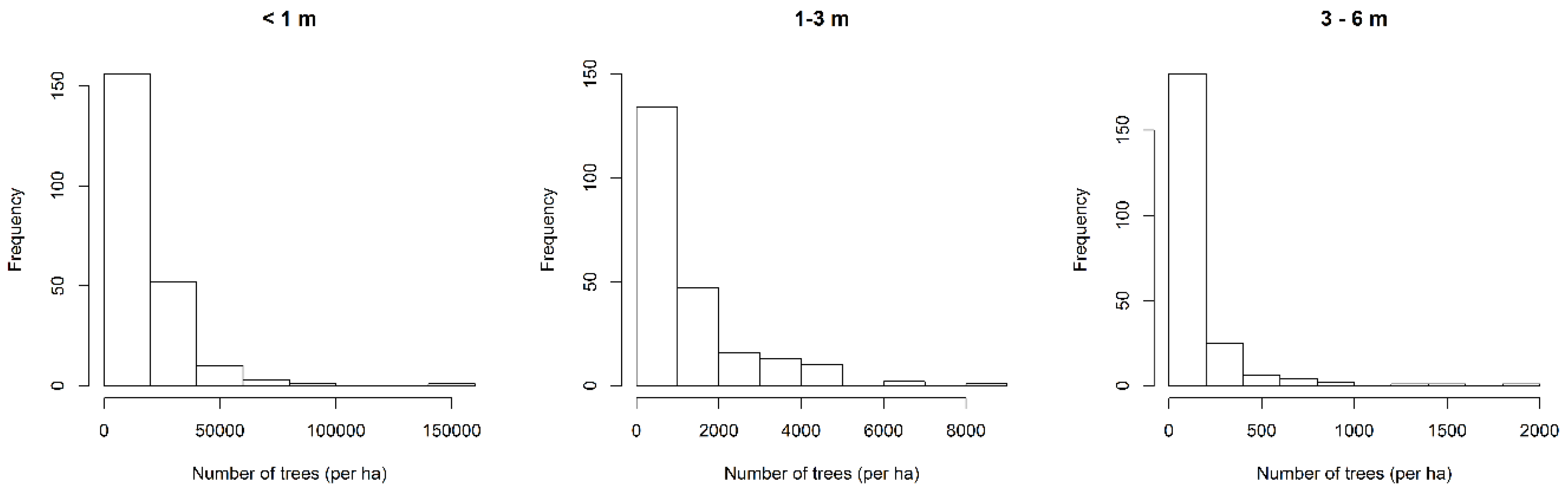
Figure 1. Location of the study area and sample plots overlaid upon a false color Landsat image.
Remotesensing 10 01446 g001
Figure 2. Field photos of DDF sample plots.
Remotesensing 10 01446 g002
Figure 3. Histogram of the number of small regenerating trees (per ha) in three height classes.
Remotesensing 10 01446 g003
Figure 4. Per plot biomass of large woody trees and small regenerating trees (in the increasing order of large woody tree biomass).
Remotesensing 10 01446 g004
Figure 5. A comparison of R2, result of RF method, between different allometric equations used in the study: (a) total AGB including small regenerating trees and large woody trees; and (b) large woody tree biomass alone.
Remotesensing 10 01446 g005
Figure 6. A comparison of NRMSE (%RMSE), result of RF method, between different allometric equations used in the study: (a) total AGB including small regenerating trees and large woody trees; and (b) large woody tree biomass alone.
Remotesensing 10 01446 g006
Figure 7. Scatterplots of observed and predicted AGB values in different variable group tests across regression methods: (a) Raw spectral bands; (b) VIs; (c) Band ratios; (d) PCs; (e) Texture; and (f) Combined variables. MLR, Multiple Linear Regression; SMLR, Stepwise Multiple Linear Regression; RF, Random Forest; SVM, Support Vector Machine.
Remotesensing 10 01446 g007aRemotesensing 10 01446 g007b
Table 1. Number of individual small regenerating trees (per ha) in three height classes.
HeightMinMaxMeanStandard Deviation
<1 m300141,10015,38517,292
1–3 m0870012191376
3–6 m02000136252
Table 2. List of allometric equations used in the study.
NoEquationsReferencesR2/R2 adjRemarks
Allometric equations used for calculating large woody tree biomass
1Equation (1)[62]0.93UN-REDD—developed specifically for deciduous forests in the Central Highlands in Vietnam
2Equation (2)[64]0.97For tropical and humid regions
3Equation (3)[2]0.97For humid regions
4Equation (4)[3]N/A
5Equation (5)[2]0.99
Allometric equations used for calculating small regenerating tree biomass
6Equation (6)[23]
B, biomass of large woody trees (kg); DBH, diameter at breast height (cm); H, Height (m); WD, Wood Density (g cm−3); Y, biomass of small regenerating trees (kg).
Table 3. Variables derived from Landsat-8 OLI.
VariablesFormulaReferences
Six raw spectral band reflectancesBand 2, Blue; Band 3, Green; Band 4, Red; Band 5, Near Infrared (NIR); Band 6, Shortwave Infrared (SWIR) 1; Band 7, SWIR 2
Seven Vegetation Indices
Normalized Difference Vegetation Index (NDVI) N I R R E D N I R + R E D [67]
Soil Adjusted Vegetation Index (SAVI) ( 1 + L ) ( N I R R E D ) ( N I R + R E D + L )
where L = 0.5
[68]
Enhanced Vegetation Index (EVI) 2.5   ×   N I R R E D N I R + 6 R E D 7.5 B L U E + 1 [69]
Difference Vegetation Index (DVI)NIRRED[70]
Ratio Vegetation Index (RVI)NIR/RED[71]
Atmospherically Resistant Vegetation Index (ARVI)(NIRRB)/(NIR + RB)
where RB = RED − 1 × (BLUERED)
[72]
Global Environment Monitoring Index (GEMI)N × (1 − 0.25 × n) − (RED − 0.125)/(1 − RED)
where n = [2(NIR2RED2) + 1.5NIR + 0.5RED]/(NIR + RED + 0.5)
[73]
Six Simple Band RatiosBLUE/GREEN
BLUE/RED
BLUE/NIR
GREEN/RED
GREEN/NIR
RED/NIR
Three Principal Component Bands (PC1–PC3)
Eight Grey Level Co-occurrence Matrix (GLCM) texture parameters
(window sizes from 3 × 3 to 11 × 11) from six raw spectral bands
Mean (ME) i , j = 0 N 1 i P i , j
Variance (VA) i , j ( x i , j μ ) 2 n 1
Homogeneity (HO) i , j = 0 N 1 i P i , j 1 + ( i j ) 2
Contrast (CO) i , j = 0 N 1 i P i , j ( i j ) 2
Dissimilarity (DI) i ,   j = 0 N 1 i P i , j | i j |
Entropy (EN) i , j = 0 N 1 i P i , j ( l n P i , j )
Second Moment (SE) i , j = 0 N 1 i P i , j 2
Correlation (CC) i , j = 0 N 1 [ ( i μ i ) ( i μ j ) ( σ i 2 ) ( σ j 2 ) ]
Pi,j is the value in the cell i, j (row i and column j) of the moving window and N is the number of rows or columns.
Table 4. In situ biomass (Mg/ha) estimated by different allometric equations.
NoEquationsReferencesMinMaxMeanStd Dev.
Large woody tree biomass
1Equation (1)[62]5.37210.3159.7031.06
2Equation (2)[64]7.37424.56102.2659.18
3Equation (3)[2]4.34264.4162.5738.36
4Equation (4)[3]4.58323.4874.7845.63
5Equation (5)[2]5.27335.4081.3148.20
Small regenerating tree biomass
6Equation (6)[23]1.08233.0162.7651.94
Table 5. Biomass distribution of sample plots, comparing different allometric equations.
Biomass Range
(Mg/ha)
Percentage of Plots (%)
Equation (1)
Percentage of Plots (%)
Equation (2)
Percentage of Plots (%)
Equation (3)
Percentage of Plots (%)
Equation (5)
Percentage of Plots (%)
Equation (4)
Large woody tree biomass
0–5042.0416.8141.5934.5129.65
50–10045.5837.1740.2739.8239.82
100–1508.4124.7812.3916.3718.14
150–2000.4412.391.774.427.08
>2000.445.750.881.772.21
Total AGB (including biomass of both large woody trees and small regenerating trees)
0–5012.833.5414.6011.509.73
50–10026.9925.2223.8924.3423.89
100–15023.4514.1623.4518.5818.58
150–20021.2423.8922.5723.0123.01
>20012.3930.0912.3919.4721.68
Table 6. AGB estimation errors in different tests with different regression models (excluding topographic variables).
Test VariablesMLRSMLRRFSVM
R2RMSE
(Mg/ha)
R2RMSE
(Mg/ha)
R2RMSE
(Mg/ha)
R2RMSE
(Mg/ha)
1Raw spectral bands0.4048.820.4148.720.3949.870.4049.76
2VIs0.3650.810.3650.520.3054.140.3651.78
3Band ratios0.3750.170.3750.180.3949.890.3751.43
4PC0.3749.890.3749.890.2755.010.3751.01
5Texture0.4049.010.4148.740.3352.230.4049.28
6Combined0.4051.230.4051.280.3849.610.4149.52
MLR, Multiple Linear Regression; SMLR, Stepwise Multiple Linear Regression; RF, Random Forest; SVM, Support Vector Machine.
Table 7. AGB estimation errors in different tests with different regression models (including topographic variables).
Test VariablesMLRSMLRRFSVM
R2RMSE
(Mg/ha)
R2RMSE
(Mg/ha)
R2RMSE
(Mg/ha)
R2RMSE
(Mg/ha)
1Raw spectral bands0.4248.060.4447.420.4846.220.4249.21
2VIs0.3750.220.3650.540.4149.120.3851.28
3Band ratios0.4049.090.3949.280.4746.420.3950.90
4PC0.3949.260.3849.580.4048.890.3950.84
5Texture0.4248.140.4048.740.4248.180.4248.66
6Combined0.4051.530.4349.670.4646.490.4248.79
MLR, Multiple Linear Regression; SMLR, Stepwise Multiple Linear Regression; RF, Random Forest; SVM, Support Vector Machine.
Table 8. Correlation coefficients between topographic variables and total field-based biomass (large woody trees and small regenerating trees) computed from different allometric equations.
Topographic VariablesEquation (1)Equation (2)Equation (3)Equation (4)Equation (5)
Elevation0.490.450.460.450.45
Slope0.470.400.430.400.39
Aspect0.030.010.00−0.03−0.03

