Remote Sensing of Antarctic Glacier and Ice-Shelf Front Dynamics—A Review

Abstract

The contribution of Antarctica’s ice sheet to global sea-level rise depends on the very dynamic behavior of glaciers and ice shelves. One important parameter of ice-sheet dynamics is the location of glacier and ice-shelf fronts. Numerous remote sensing studies on Antarctic glacier and ice-shelf front positions exist, but no long-term record on circum-Antarctic front dynamics has been established so far. The article outlines the potential of remote sensing to map, extract, and measure calving front dynamics. Furthermore, this review provides an overview of the spatial and temporal availability of Antarctic calving front observations for the first time. Single measurements are compiled to a circum-Antarctic record of glacier and ice shelf retreat/advance. We find sufficient frontal records for the Antarctic Peninsula and Victoria Land, whereas on the West Antarctic Ice Sheet (WAIS), measurements only concentrate on specific glaciers and ice sheets. Frontal records for the East Antarctic Ice Sheet exist since the 1970s. Studies agree on the general retreat of calving fronts along the Antarctic Peninsula. East Antarctic calving fronts also showed retreating tendencies between 1970s until the early 1990s, but have advanced since the 2000s. Exceptions of this general trend are Victoria Land, Wilkes Land, and the northernmost Dronning Maud Land. For the WAIS, no clear trend in long-term front fluctuations could be identified, as observations of different studies vary in space and time, and fronts highly fluctuate. For further calving front analysis, regular mapping intervals as well as glacier morphology should be included. We propose to exploit current and future developments in Earth observations to create frequent standardized measurements for circum-Antarctic assessments of glacier and ice-shelf front dynamics in regard to ice-sheet mass balance and climate forcing.

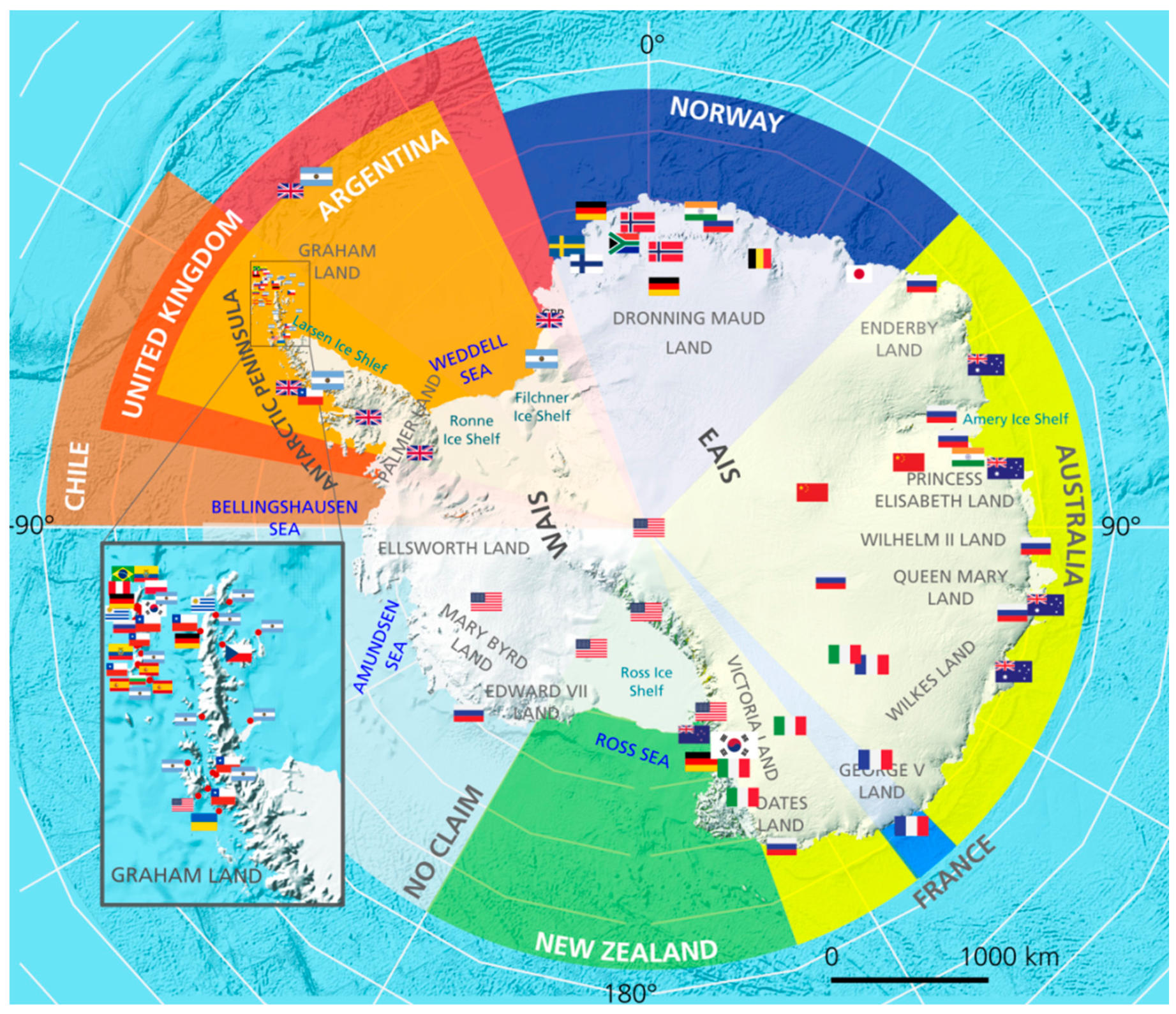
1. Introduction: Relevance of Antarctica and Scope of this Review

Antarctica is a continent of superlatives. The Antarctic ice sheet stores about 91% [1] of the global glacier ice on an area of 13.9 × 10³ km² [2]. If the Antarctic ice sheet melted completely, this mass loss would raise our global sea level by 58.3 m [3]. Between 1992–2017, the annual mass loss of the Antarctic ice sheet was −109 Gt/yr ± 56, which was equal to a rise of 0.3 mm/yr in sea level [4]. Most of the grounded ice lost, 80%, is lost to the ocean by basal melting or calving. The Antarctic coastline has a length of about 43,449 km [5], which is longer than the circumference of the Earth, with 75% of the coastline being ice shelves, which cover an area of 1.56 × 10⁶ km² [6]. Besides huge ice shelves, innumerable smaller glaciers are located along the Antarctic coast. So far, the total number of Antarctic glaciers is unknown, but rough estimates range from 2752 [7] to 3274 glaciers [3].

Interest in Antarctica is not only limited to the cryosphere, as Antarctica is endowed with valuable resources such as metallic and non-metallic minerals, as well as fossil fuels [8,9]. Natural resources deplete on a global scale and the tense situation might even extend to Antarctica. Currently, the Antarctic Treaty preserves the territorial status quo and prohibits mining, but depleting resources might ignite new conflicts on territorial claims [10]. According to the Antarctic Treaty [11], the Antarctic territory stretches from 60° S latitude to the South Pole with the highest elevation at Vinson Massif 4897 m [12]. The Antarctic Treaty is signed by 12 states, with seven of them claiming land [13]. Antarctica is occupied by 100 open research facilities run by 30 different nations as counted by COMNAP (Council of Managers of National Antarctic Programs, March 2017).

Figure 1 shows the territorial claims on Antarctica and the location of seasonal and year-round research facilities. Additionally, the map gives an overview of the important Antarctic regions and ice shelves that are mentioned later in the text.

Antarctica will not only become more important in the context of a worldwide struggle for resources, but also in the context of global change. Warming temperature trends put pressure on the ecosystem, at least at the West Antarctic Ice Sheet (WAIS) and the Antarctic Peninsula (AP) [14]. In addition, the human impact on the fragile ecosystem is emerging through illegal fishing activities, whaling, exploitation for bioprospecting purposes, and a flourishing tourism industry [13,15,16]. Changes in the Antarctic ecosystem influence many factors such as sea level, climate, and biochemical cycles, as well as the thermohaline circulation on a global scale with teleconnections that are not fully understood yet.

One process that is relevant to sea level is the dynamic fluctuation of the Antarctic glacier and ice-shelf front locations [15,16]. In some regions, remote sensing imagery reveals huge icebergs breaking up along Antarctica’s coastline and ice shelves disintegrating, whereas in other areas, advancing glaciers can be observed. For Antarctica, the processes controlling the calving of marine-terminating glaciers and ice shelves are only partly known [17,18]. Existing studies have either analyzed fronts of (i) individual glacial features with very high spatial and temporal resolution [19,20,21], (ii) larger regions of the Antarctic coastline at a lower temporal resolution [22,23,24], or (iii) the entire Antarctic coastline for single years based on entire satellite imagery mosaics [25,26,27].

Depending on the study design (region of interest, observation timespan, interval of observation, spatial coverage), the reasons for retreating and advancing fronts are attributed to different drivers [22,24,28,29,30]. However, no review paper exists that allows a comprehensive overview on available ice shelf and glacier front positions along the Antarctic coastline. Hence, circum-Antarctic front fluctuations cannot be assessed, as the findings of different studies have not yet been brought together. With this review, we provide for the first time an overview on all of the existing Antarctic calving front studies to address the following research questions:

• How can calving front dynamics be measured based on remote sensing imagery?
• How good is the circum-Antarctic data availability of glacier and ice-shelf front positions?
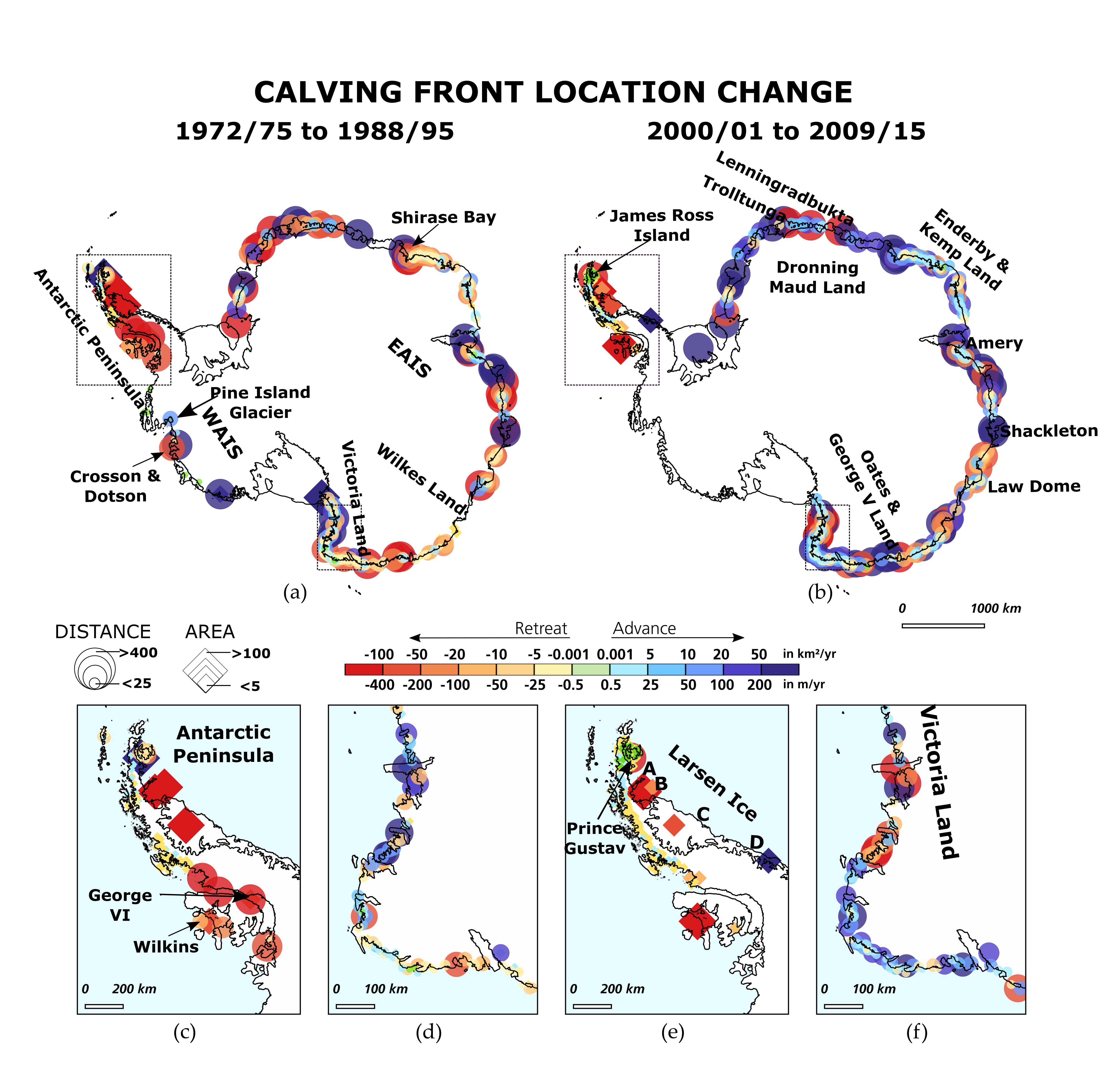
• What circum-Antarctic patterns of retreating and advancing fronts can be observed?

The review also gives insight into the common control mechanisms of calving and processes influencing the frontal positions of glaciers and ice shelves. The role of remote sensing in mapping and analyzing calving fronts will be examined, and finally, the results of the compiled dataset are presented to show the available data and circum-Antarctic patterns in calving front fluctuations.

2. The Importance of Calving Front Dynamics

A calving front is defined as the location where the ice sheet ends and the ocean or sea ice begins [31]. Ice shelves and glacier tongues are seen as floating extensions of an ice sheet. It should be noted that different sea ice types exist that are occasionally visually difficult to distinguish from land ice. Perennial sea ice or fast ice (sea ice “fastened” to land and not moving with tides) might appear very similar to shelf ice in remote sensing imagery [32]. The different morphologies of the fronts and various manifestations of sea ice are displayed in Figure 2.

In the literature, the term “front” can also be substituted with terminus [33,34], margin [24], calving front [35], or barrier [36]. The term ice wall is only used if the front is not floating on top of the ocean, but rather grounded on rock [1]. Together, the locations of ice shelf and glacier fronts can be summarized by the shorter term, calving front location (CFL). Changes in CFL can be determined either by the distance between an arbitrary specified point and the front over a given time [37] or by changes in the area between a box outline and the delineated CFL [38]. Studies on CFL fluctuations are also often referred to as studies on coastal change [39,40] or changes in glacier/ice-shelf front extent [32].

Glacier and ice-shelf fronts are of a dynamic nature, as the floating ice flows seawards until the yield strength of the ice is reached [41]. Ice breaks off if its strain rate gets too high and fracture processes initialize the formation of icebergs (Figure 2d–f) [42]. Hence, the CFL retreats with iceberg calving as soon as the iceberg is no longer fastened to the glacier tongue or shelf ice. Calving is one important mass loss component of the Antarctic ice sheet, accounting for almost half of the entire mass loss. The other half is attributed to basal melt [6,43,44]. For Antarctica, surface melt can be seen as a minor mass loss component, and is so far not of major importance compared to calving and basal melt [45].

The dynamical behaviors of glacier termini and ice-shelf fronts are linked to climate forcing, ocean forcing [24,46], and internal ice-sheet dynamics [28,47]. Enhanced basal melting thins the floating ice, and iceberg calving increases as yield strength decreases [27,41,48]. A loss of floating ice can decrease the buttressing effects, which are followed by enhanced ice discharge [41,46,49]. The magnitude of ice discharge acceleration and possible grounding line retreat is closely connected to the slope of bed topography [41,48]. For example, faster ice flow velocities have been observed after the disintegration of the Larsen B ice shelf for its tributary glaciers [50]. This cascading effect shows that the buttressing effect of ice shelves and glacier tongues has a major influence on the ice sheet discharge, and thus the Antarctic mass balance.

To quantify the contribution of an ice sheet to rising sea levels, it is essential to improve the understanding of iceberg calving and the driving forces behind ice loss [18,46,51], as well as the use of dynamic ice shelf and glacier fronts in mass balance calculations [27] and ice sheet models [52].

Calving is a very complex process, as calving can trigger the acceleration of ice flow, but internal ice dynamics may also change the process of calving [17]. When studying calving fronts, it is important to bear in mind that glacier behavior is very different from case to case, as not only internal ice dynamical factors, but also external factors (e.g., bed topography, climate) influence the calving rate and front fluctuation. Existing studies have linked atmospheric and oceanic warming to enhanced iceberg calving and retreat by studying the fluctuation of glacier and ice-shelf front positions [15,28,29,44]. Changes in calving front location are seen as an early sign for further ice dynamical changes [53]. Nevertheless, climate forcing may not be the sole driver, since the “natural” cyclic behavior of calving needs to be considered [17,24,54,55], as well as the type of terminus [28,51]. Recent studies of outlet glaciers in Greenland and Svalbard indicate that ocean forcing and climate forcing at the terminus are the factors principally determining calving changes, rather than ice-sheet dynamics [18,56]. Monitoring and analyzing changes in retreating and advancing fronts is necessary in order to identify the driving forces behind CFL dynamics for Antarctica as well.

3. Review on the Remote Sensing of Calving Fronts

The review on Antarctic calving front studies using airborne and/or satellite remote sensing data is based on 114 relevant SCI (Science Citation Index) papers identified by a systematic literature search. For each reviewed study, several parameters were analyzed, such as applied sensors, study topic, research motivation, studied glacial features, applied methodology, and the spatial coverage of the study area. In addition, each measured retreat or advance of a glacier/ice-shelf front was combined into one single dataset. Further details on the systematic review are provided in Figures S1 and S4 and Table S1 in the Supplementary Section. The results of the review on the remote sensing of Antarctic calving front studies are structured in the following way. First, the appearance of glacier and ice-shelf fronts in optical and radar satellite imagery is outlined before introducing applied methods to measure calving front dynamics from remote sensing imagery. The reviewed studies are categorized afterwards, and the spatial and temporal availability of CFL studies is presented. Finally, cirum-Antarctic patterns of glacier and ice-shelf front changes are presented based on the generated dataset.

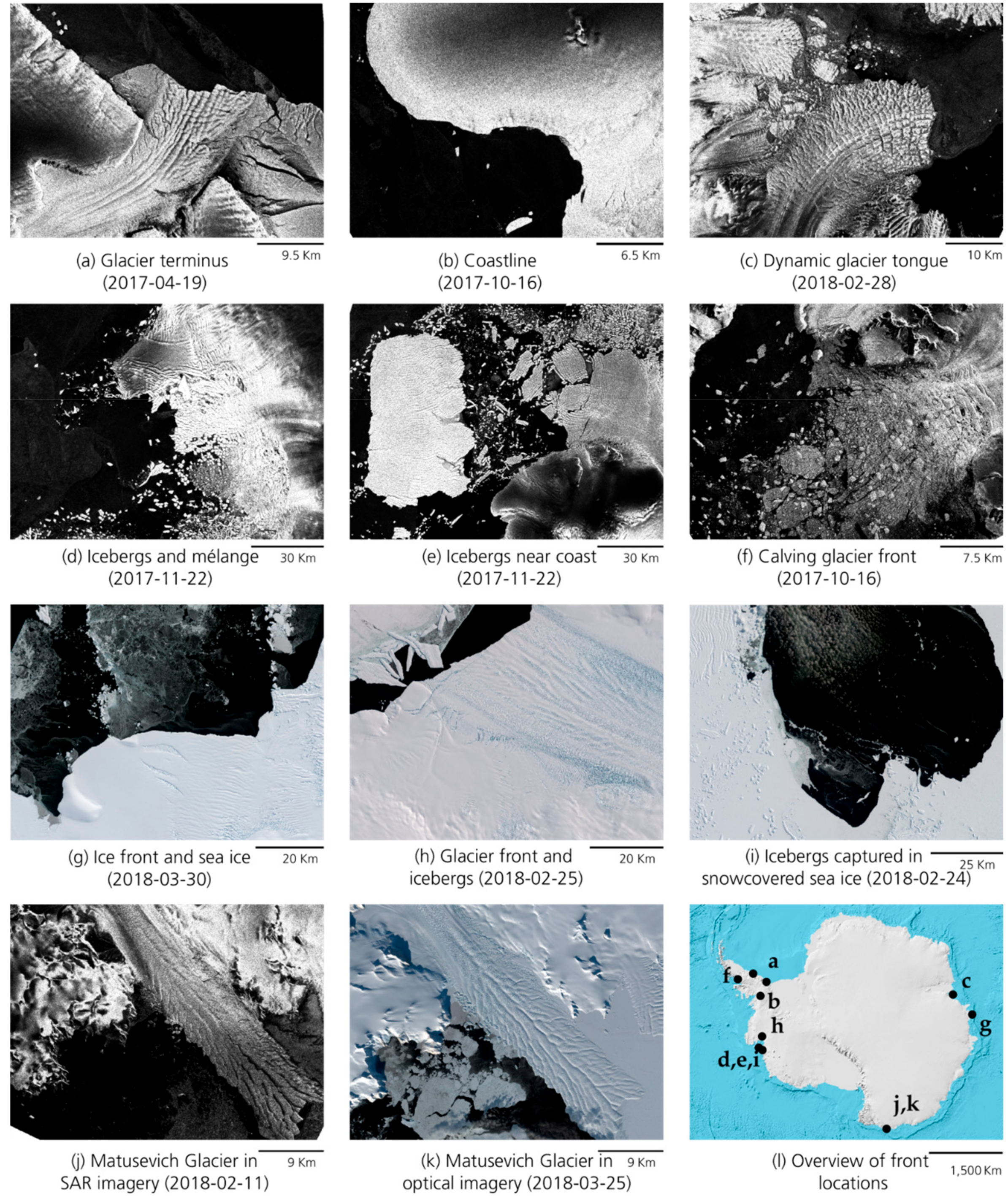
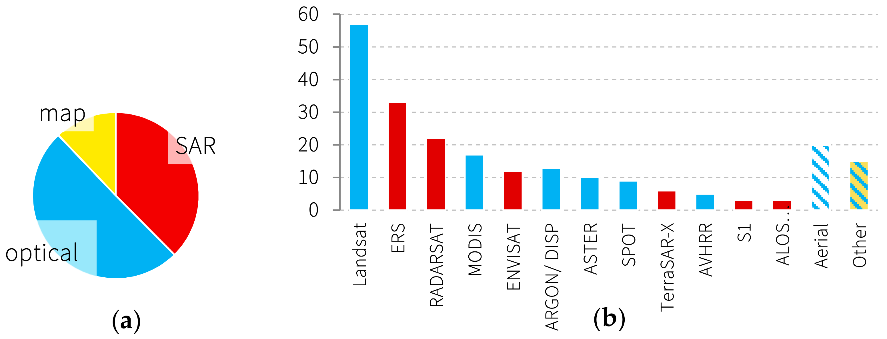
3.1. Remote Sensing of Calving Fronts with Optical and SAR Sensors and Applied Sensors

The extraction of ice shelf and glacier fronts from optical and synthetic aperture radar (SAR) satellite imagery requires the identification of the spectral and physical properties of glacial features. The front can be extracted as the boundary between two enclosing classes: land and water. In the case of Antarctica, this raises classification challenges that are known both for ice sheets due to snow melt [57,58] and ocean seasonally covered by sea ice [59,60,61]. Throughout the year, backscatter characteristics and reflectance spectra of the ice sheet and sea ice surface vary [62,63] (an example is given in Figure S2 in the Supplementary Material). Additional challenges are wind roughening in SAR scenes [26], clouds in optical imagery [64], the spectral similarity of sea ice, fast ice, and shelf ice [65] (see Figure S3 for reflectance spectra of ice, snow, and clouds), and icebergs surrounded by sea ice (mélange) [62]. Ice sheet signatures vary due to different glacier facies and extensive snow melt in summer [66], whereas sea ice appears differently depending on salinity, air content, and temperature [62]. Excellent knowledge about the spectral and physical properties of all kinds of Antarctic ice and the snowpack on top is essential for exact definitions of calving fronts. A brief summary of the advantages and disadvantage of both imaging techniques is given in

Table 1. Comparison of advantages and disadvantages for calving front location (CFL) extraction in optical and synthetic aperture radar (SAR) imagery.

Variable	Optical	SAR
Accuracy	High spatial accuracy and often higher resolution	Lower spatial accuracy
Data Availability	Low scene availability due to polar night and heavy cloud cover	High scene availability due to light independence and penetration of clouds
Snow and Clouds	Similar reflectance of snow and clouds for some wavelengths	Penetration of clouds and thin snow cover
Ice	Different spectral bands allow separation of ice features [67,68,69] Separation of shelf ice and fast ice sometimes challenging due to snow cover.	Change of backscatter values during the year (glacier facies) [58,63,70] Different ice types might have similar backscatter values
Additional	Even for non-experts, fronts are easy to distinguish	Wind roughening of the ocean surface [71]. High contrast for water–ice boundary [5]. Shadow, layover, incident angle, penetration depth

.

During the review process, it was identified that 50% of all of the reviewed studies use optical imagery (including aerial flight campaigns), whereas SAR data is used in one-third of the studies (Figure 3). Also, geographical maps seem to be a valuable data source, with a share of almost a sixth of the reviewed studies. Antarctic maps usually date back further in time, as they often include CFLs from mapping expeditions and aerial photography.

The 12 most commonly applied satellite missions are displayed in Figure 3. Landsat is the most used satellite mission. A few reasons for the prevalent popularity of Landsat include its continuous time-series since the 1970s up to Landsat-8 today, open data access, medium-resolution imagery and pre-processed scenes. Landsat is closely followed by ERS (European Remote Sensing Satellite) and RADARSAT (as the most applied SAR sensors. The ERS mission is one of the first operational SAR sensors with records since the early 1990s, which were prolonged by the ENVISAT mission with a higher repeat pass providing an abundance of scenes for creating three-day mosaics with a resolution of 1 km [72]. RADARSAT is also widely used, as two complete mosaics with delineated coastlines exist for 1997 and 2000 with a medium resolution of 30 m (Standard Mode). Moderate Resolution Imaging Spectroradiometer (MODIS) imagery is widely used, even though its spatial resolution is low. The lower spatial resolution is compensated by the high temporal resolution with a daily revisit cycle [73]. This increases the probability of acquisitions without clouds. The imagery of the United States (US) Declassified Intelligence Satellite Photographs (DISP) is widely used, even though orthorectification and geolocation errors are frequent. In particular, mission KH-5 (ARGON) provides valuable coastline information, as Kim et al. (2007) [74] managed to process a comprehensive mosaic of the ARGON imagery for the year 1963. High-resolution imagery from missions such as TerraSAR-X, SPOT, or Quickbird/WorldView (category “other”) is used less frequently. This is probably connected to the small spatial coverage and high image cost. So far, Sentinel-1 imagery has only been utilized in a few studies. Within the next few years, the usage of Sentinel-1 data will probably increase as more acquisitions over a longer timespan will be available in the future. The value of optical imagery from Sentinel-2 has not yet been fully exploited, as only some of the imagery has been used by the Antarctic Digital Database (ADD) to delineate front locations.

The abundance of used sensors and the combination of aerial, optical, and SAR images in most studies stands for the paradigm of “use all data you can get”. Only if different data sources are combined can long time-series with large coverage and high observation intervals be achieved.

3.2. Methods to Extract Calving Fronts from Satellite Imagery

The most applied method to extract glacier termini or ice-shelf fronts is the manual delineation from georeferenced imagery with geoinformation software. This technique has been applied for 85% of the reviewed studies, and works well independently from data source and sensor type. Only 7% of CFLs were extracted automatically or semi-automatically, whereas 8% of the studies used already existing CFL datasets from previous studies. Even huge projects such as the coastline of the MODIS mosaic [25] or the United States Geological Survey (USGS) mapping project were produced manually [40]. Still, the most up-to-date Antarctic coastline provided by the Antarctic Digital Database (ADD) is mostly updated by manual delineated datasets. However, in times of rapidly growing satellite image archives, the big disadvantage of manual work—a high expenditure of time—becomes a real issue, and new approaches have to be developed. The automated front extraction finds its origin in the shoreline or coastline extraction [71,75].

There are many similarities to front extraction, but seasonal variations in ice types require especially modified approaches. Several attempts have been made to develop simplistic semi-automatic approaches in order to pre-delineate the CFL before manual revision (e.g., Liu et al. 2015 [27]). There have also been attempts to develop fully automated techniques of front extraction for specific imagery such as MODIS [54] or RADARSAT [26]. However, so far, no automatic algorithm exists that accurately extracts fronts without the necessity of manual post-corrections. Besides Antarctic approaches, some promising techniques for Greenland are also mentioned, as the front extraction challenges are mostly similar. Every mapping approach has advantages and disadvantages, which are summarized in

Table 2. Advantages and disadvantages of different CFL mapping techniques.

	Manual	Semi-Automatic	Automatic
Advantages	Applicable for every image type Quick for single glaciers Very accurate and precise Even “difficult” fronts can be mapped by experts	Less manual work Mapping large regions is possible	Quick, even for a large amount of scenes Monitoring possible
Disadvantages	Time-consuming Subjectivity of the observer Expert knowledge for difficult fronts necessary Not suitable for large-scale application	Manual post-processing still necessary Restricted to one sensor Expert knowledge for difficult fronts necessary	Not always accurate Long duration for algorithm development Only applicable for one sensor Computational cost is high

. A summary of the references for existing front extraction algorithms is given in

Table 3. Comparison of automatic (A) and semi-automatic (SA) calving front extraction approaches.

Study	A/SA	Based on	Image Processing Techniques	Test Area	Years and Amount of Data	Error	Difficulties
Sohn and Jezek 1999 [78]	A	ERS-1	Edge enhancement Texture features Local thresholding Edge detection with Robert operator	100 × 100 km 37.5 × 37.5 km Jakobshavn Glacier	1988 + 19922 Scenes	2–3 pixels 200 m	Lakes and outwash plains Sensor inaccuracies
		SPOT					Thin snow
Seale et al. 2011 [54]	A	MODIS	Cloud masking Edge detection with Sobel operator + brightness gradient Removal of wrong data points via time-series	32 glaciers 26802 fronts Greenland	2000–2009 105,536 Scenes	1.2% of data points wrong	Polar night and clouds Sensor inaccuracies Direction of scene
Klinger et al. 2011[65]	A	LIMA 1 Mosaic	Initial coastline + classification with nearest neighbor Three snake models with different parameters and edge detectors	12% of Antarctic coastline	1999–2003	6% of sections had to be corrected 12.1% false negative 13.7 false positive 1.5 pixel or 380 m	Initial coastline needed Sea ice to shelf ice boundary No greater change than 2 km allowed Manual post-processing necessary
Krieger and Floricioiu 2017[79]	A	TerraSAR-X Sentinel-1	Canny edge detection Shortest path between edge candidates	Zachariae Isstroem	2016 + 2017 2 Scenes	Mean distance between Expert and Automatic 246 m + 159 m	End and start point have to be specified for each glacier More diverse test areas are required
Liu and Jezek 2004 [5]	A	Landsat 7	Pre-segmentation Segmentation Post-segmentation	212 × 226 km	1 Scene	One pixel (compared to visual interpretation)	Fast ice, sea ice, and wet snow Fixing errors in ArcGIS For optical imagery, perfect
		RADARSAT		409.6 × 409.6 km	1 Scene
Wu and Liu 2003[76]	SA	RADARSAT	Feature detection Wavelet transform Edge detection Texture for classification	Bering sea400 × 400 km	2000 1 Scene	-	Also detects ice edge Parameterization Static thresholds No error calculation
Liu et al. 2015[27]	SA	ENVISAT ASAR	Object-based classification Watershed segmentation Manual modifications	Circum- Antarctic	2005–2011	Visually corrected	Manual work afterwards
Liu and Jezek 2004 [5] Liu et al. 2004[26]	SA	RADARSAT Mosaics AMM 2 and MAMM 3	Lee filter for edge enhancement and speckle reduction Segmentation with local adaptive threshold Canny edge detector Manual editing and merging	Circum- Antractic	1997 + 2000 Entire mosaic	130 m (DEM) Visually corrected version available	Wind-roughened sea Sea ice Orthorectification
Miles et al. 2017[46]	SA	ENVISAT, ASAR	Pixel-based classification Polygon generation	Coastal Section	Monthly scenes 2002–2012	45% had to be manually corrected	Only 65% were automatically mapped precisely

¹ Landsat Image Mosaic of Antarctica, ² Antarctic Mapping Mission, ³ Modified Antarctic Mapping Mission.

.

3.2.1. Semi-Automatic Approaches

Wu and Liu (2003) [76] extracted ocean features such as ice edge, polar lows, and ice fronts with traditional image processing techniques such as greyscale histograms, texture analysis, and wavelet transforms for edge extraction. Edges were detected, but the accuracy of the extracted front is pretty generalized, and thresholds for classifications as well as initial parameters for the wavelet transform have to be parameterized manually. Much more promising is the approach of Liu and Jezek (2004) [5,26], which was implemented for the RADARSAT Mosaic of Antarctica from 1997. After applying a Lee filter for speckle reduction and an anisotropic diffusion algorithm for edge enhancement, regions with high variance can be chosen to detect edges by a Canny edge detector. The Levenberg–Marquardt method is used to iteratively fit the bimodal distribution, which is mostly a combination of two Gaussian distribution functions [26]. For the bimodal distribution, a locally adaptive threshold can be computed. The image can then be segmented by the threshold and classified into the classes land and water. The final coast can be traced after post-processing, where misclassifications are smoothed out. This approach is already highly automated and almost no manual work is necessary, although still, classification errors between shelf/glacier ice and sea ice still exist [26].

Recent studies chose more simplistic automated approaches to assist manual editing [27,46,77]. Liu et al. [27] developed an object-based classification algorithm based on a watershed segmentation to roughly distinguish different land classes. Final manual revision and editing was still essential, as this approach was just used to minimize the manual work, but was not aiming for complete automatization. A similar approach was taken by Miles et al. (2017) [46], who did a pixel-based classification of SAR scenes to generate polygons for shelf ice and sea ice and define the CFL as the line in-between. The threshold for classification was calculated automatically based on the pixel statistics of each scene. Similar to Liu et al. [27], much manual work was necessary, because only 65% of the fronts could be mapped automatically without further manual editing.

3.2.2. Automatic Approaches

Not many researchers have tried to develop fully automatic approaches due to the difficulties in classification that were mentioned in Section 3.1. Sohn and Jezek (1999) [78] developed a promising technique based on classic image processing techniques for optical and SAR data. They extracted edges via the Robert operator based on edge-enhanced scenes and texture features of the SAR scene via locally adaptive thresholding. The method works well in areas where physical parameters only slightly differ because local thresholds are considered. Nevertheless, detection errors occurred in the case of a thin snow layer on the ice. Under those conditions, it was difficult to detect the front when using optical imagery. Unfortunately, the approach was only tested for a small study area, and no information on usage opportunities for large-scale applications was given. In addition, seasonal variations of sea ice and more difficult ice conditions weren’t considered. Promising results came in a study by Krieger and Floriciocu [79] for automated front extraction. However, the approach was only tested for the Greenlandic glacier Zachariae Isstroem. They used a Canny edge detection algorithm and defined start and end points of the glacier width. A tracing algorithm creates a chain along the closest detected edges. The automatically extracted CFL is consistent with the validation data (front delineated by an expert), even in areas of challenging ice conditions. So far, a large-scale validation of this approach is missing.

Besides those local approaches, two large-scale studies on front extraction exist. Seale et al. (2011) [54] managed to process MODIS scenes for 10 years along the Greenlandic coast. The challenges they had to face included a reduced availability of scenes due to polar night and the occurrence of clouds. Hence, prior to classification, a cloud mask has to be generated. A multi-temporal analysis allows the definition of active regions. For those regions, the Sobel operator and brightness gradient are applied to detect edges. A final removal of erroneous data points could reduce the inaccuracy to a minimum of 1.2% incorrect points. The developed methodology allowed a large-scale analysis, but still encountered difficulties in shelf ice and sea ice distinction. Additionally, each satellite image has to be orientated correctly, as glacier flow has to be in the same direction for classification. The only fully automated approach for Antarctica is based on active contours (also known as “snakes”) [65]. This technique is based on an initial coastline that is “pulled” toward the new front position based on classification parameters. A prior classification of features with nearest neighbor allows for the distinction of different transition zones between water, shelf ice, and sea ice. For each transition zone, a snake model was developed and applied. However, the problems include the necessity of an initial coastline (in this case provided by the RADARSAT mosaic), the allowance of a maximum change of 2 km, and the computing cost for snakes. As 6% of the analyzed sections had to be reclassified, the author still suggests manual correction. To conclude, all of the mentioned automated approaches were not able to perform well without manual post-corrections.

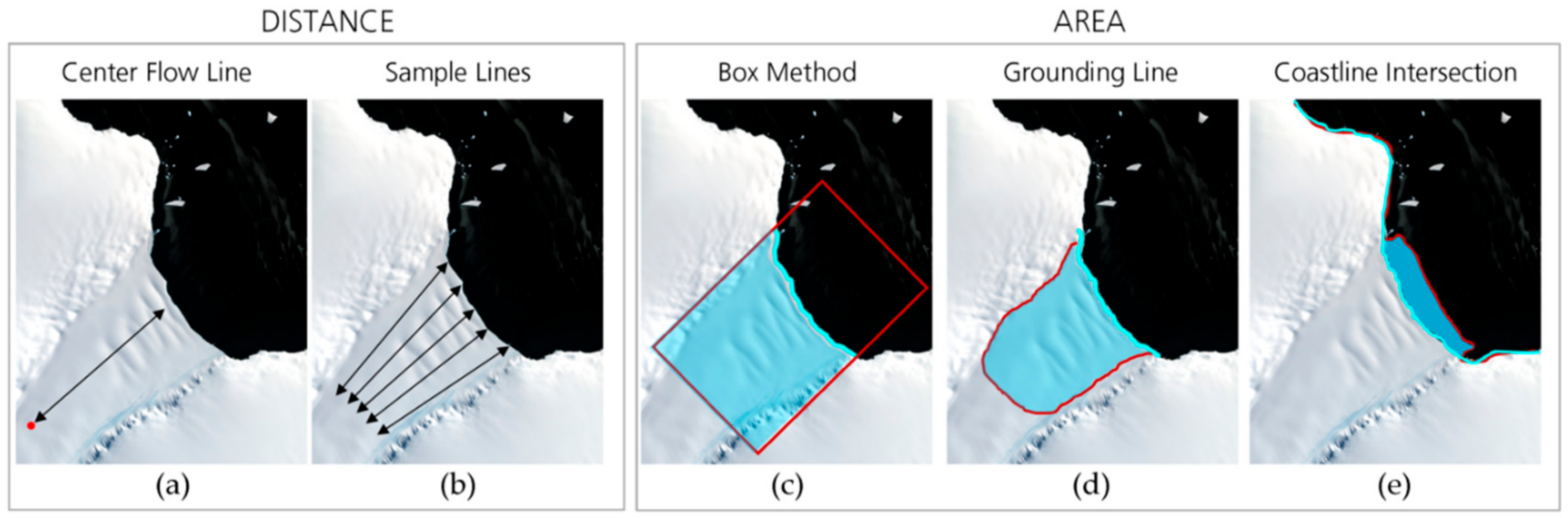
3.3. Methods to Measure Calving Front Dynamics

Measuring outlet glacier and ice shelf dynamics by tracking terminus positions is a commonly accepted approach [15,22,28,53]. A wide range of methods for glacier change monitoring is available [80]. The different approaches are visualized in Figure 4. Hence, when comparing results of different studies, it is essential to consider the method that is used for measuring advance and retreat. In the past, the most commonly used and straightforward method is the centerline technique. The distance from one fixed point along the center flow line to the terminus is measured (e.g., [81,82]). As the front position changes unevenly across the entire front, this method should only be applied to outlet glaciers with straight fronts. To also account for changes at the front margins, a good approximation is to use several lines (“sample lines”) instead of only one. The sample lines have to be placed in a flow direction parallel to each other. The front change can be calculated by averaging the measured distances along the sample lines. This method is much more accurate than the single centerline approach, and still does not need any areal calculations. The more lines that are used, the better the accuracy of the results. This improved centerline approach was used for the USGS coastal-change project [83], and is still used in up-to-date studies such as Fountain et al. 2017 [22].

As an alternative to only measuring the retreat/advance rate in meters, glacier dynamics can be expressed via areal measurements. The “box method” enables the calculation of change within a given boundary, ideally covering the entire ice body [80]. As it is very accurate and still simple, this method is widely used in many studies (e.g., [15,46,53,84]). Instead of using a bounding box, it is also possible to assume a steady grounding line and calculate the area between this and the terminus [38]. The glacier change area can also be calculated by using the entire glacier basin as a reference, which allows a good estimation of glacier change relative to its size [85,86]. For large-scale analysis along coastal sections or circum-Antarctic studies, the easiest approach is to calculate the area change between the delineated coastlines of different satellite imagery mosaics [27,87]. A deeper insight into the methodology to track glacier terminus change is given by Lea et al. [80].

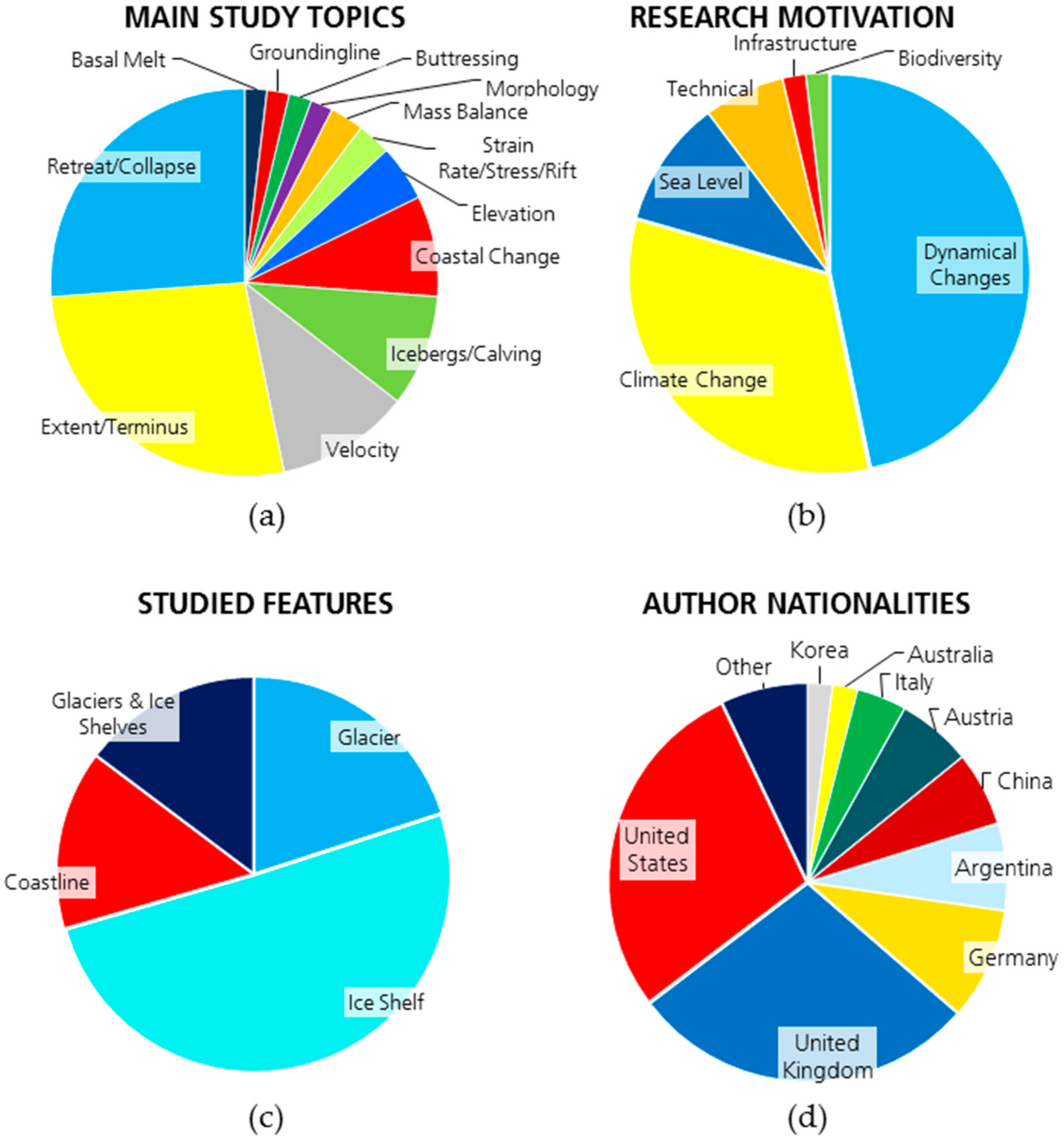
3.4. Categorization of Calving Front Studies

The reviewed studies are categorized in order to identify study topics and research motivation, as well as find links between author nationality and Antarctic territorial claims. The main study topics associated with the calving front location are presented in Figure 5a. Half of the studies examined either just the extent of glaciers and ice shelves or specific retreat or disintegration events. The location of the calving front was either used in combination with velocity measurements or to describe coastal change. Only a smaller amount of studies investigated morphological mechanisms such as strain rates and elevation changes. Buttressing effects, grounding line retreat, and basal melt all played a role, especially regarding mass balance equations.

The two main motivations for research are climate change and ice dynamical changes (see Figure 5b). Almost half of the studies aimed to investigate the dynamical changes of ice shelves and glaciers, and wanted to explain the observed changes in CFL. Secondly, the connection between climate change and its impact on calving front fluctuations drives CFL research. Related to this is also the interest in sea-level rise and how retreating fronts increase ice discharge. Of minor interest is the effect of changing fronts on infrastructure. For example, Anderson et al. 2014 [88] investigated how vulnerable the Halley Research Station is to the calving events of the Brunt Ice Shelf. Two of the reviewed studies examined effects on the ecosystem by studying ice shelf retreat followed by an increased exposure of open water [89,90]. Seven percent of the studies investigated methodical applications e.g., algorithm development, in order to extract the CFL more efficiently [91,92,93].

Of the topics described above, ice shelves are the most studied glacial feature. Half of the studies explicitly investigated ice shelves, and one-fifth investigated glaciers. The remaining 30% are coastline studies (14%) or investigations on both glaciers and ice shelves (see Figure 5c). Ice shelves are of high interest, as disintegration events are studied intensively; also, basal melt beneath ice shelves is of great interest (e.g., [94,95,96]). The study of glaciers in combination with ice shelves is done to investigate CFL fluctuations on entire coastal sections or assess the influence of instable ice shelves on their tributary glaciers (e.g., [33,97]). Most of the studies were published by British or US American researchers (see Figure 5d). The British look back on a long history of CFL studies connected to the British Antarctic Survey. Cook, Vaughan and Pritchard contributed significant studies [24,29,98]. In the US, Ferrigno and Williams provided abundance studies in the context of the USGS (United States Geological Survey) mapping project, as did Scambos with his working group at the University of Colorado. Austria had strong research interest in the late 1990s/early 2000 by the research group of Rack and Rott, which cooperated with the Argentinian research group of Skvarca. Also, Italy was active in this period with a research group led by Frezzotti and Polizzi. Since 2010, various studies of German and Chinese scientists have also been published.

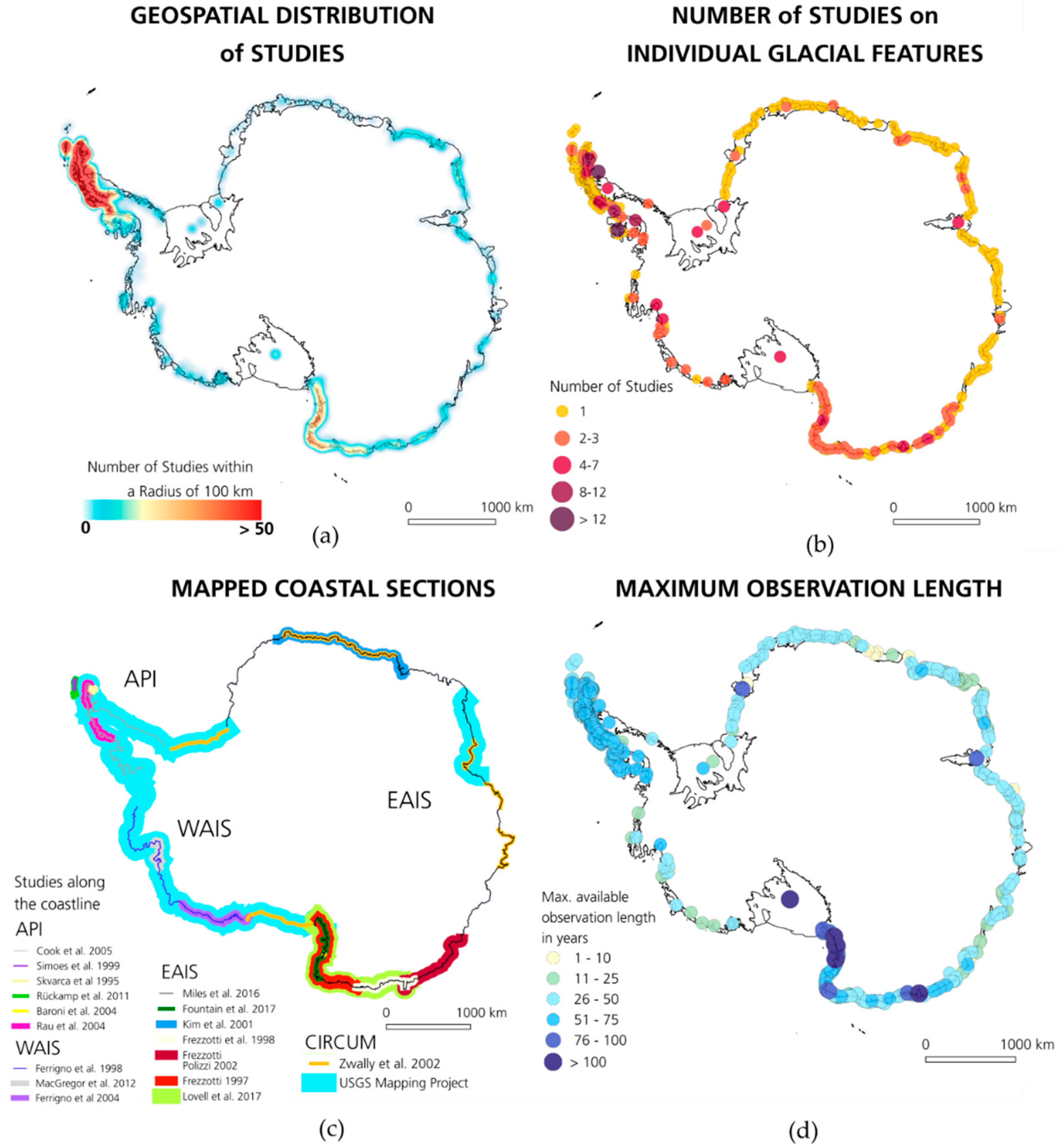
3.5. Geospatial Agglomeration and Coverage of Calving Front Studies

The spatial availability of calving front studies is displayed in Figure 6a. This heatmap indicates regions of an agglomeration of calving front studies along the Antarctic coast. Red areas indicate a higher concentration of studied glaciers and ice shelves within a radius of 100 km, blue areas indicate fewer studies. In order to calculate the spatial agglomeration of CFL studies, one point per studied glacier/ice-shelf front is plotted for each reviewed study. In case of delineated fronts for entire coastal sections, one point per glacier catchment is recorded. Front locations of King George Island, the Antarctic Peninsula, and Victoria Coast belong to the most studied regions [22,23,28,29,99,100,101]. This might be connected to the presence of numerous marine-terminating glaciers in those regions. They are very sensitive to ocean and climate forcing, and are therefore very dynamic [22,24,29]. The agglomeration of studies seems also to be connected to the territorial claims. For the unclaimed WAIS, considerably fewer CFL studies exist than for the other claimed parts of Antarctica. Also, the studies by specific nations are related to their claimed parts and research stations. For example, Argentina and the United Kingdom concentrate their studies mostly on the AP. Italian researchers often chose their study area along Victoria Land, which is close to their research station Mario Zucchelli. The United States, which has not claimed any land, concentrated their studies along the unclaimed WAIS. A low density of studies exists for the ice shelves of Dronning Maud Land, parts of Wilkes Land, and the glacier fronts terminating into the Bellingshausen Sea. The distribution of highly mapped regions versus poorly mapped coastal sections might be connected to data availability. This should be further investigated by a data availability study.

The reviewed studies not only vary significantly in their spatial distribution, but also in their spatial coverage. Calving front studies can be categorized into three main spatial scales:

• Local case studies
• Regional studies
• Circum-Antarctic coastline studies

Small-scale studies account for the largest share, as 63% of the reviewed studies only investigate single glaciers or ice shelves. A further 27% of the reviewed studies assessed calving front fluctuations along larger coastal sections. The smallest proportion of studies covers the entire Antarctic coastline with a share of 10%.

3.5.1. Local Calving Front Studies

Local calving front studies concentrate on a few popular glaciers and ice shelves, as can be seen in Figure 6b. The front of the Larsen B ice shelf, with 27 studies, is the most studied feature of Antarctica. Also, the fronts of the Wilkins, Larsen A, Larsen Inlet, and Prince Gustav ice shelves are favored study objects, with 12, 12, 11, and 10 studies, respectively. The high interest in the Larsen Ice Shelf can be attributed to the disintegration of Larsen A and Larsen B, as well as the huge calving events of Larsen C [102,103,104,105]. Also, for the Wilkins Ice Shelf, a strong retreat since the 1990s was detected on satellite imagery before its partial disintegration in 2008/2009, which resulted in many studies [106,107]. The disintegration of the Larsen ice shelves reduced the buttressing for the feeding glaciers, which accelerated and retreated beyond the grounding line. [108]. This type of front retreat directly contributes to sea-level rise.

Besides Larsen and Wilkins, the Ronne-Filchner ice shelf is the third most studied ice-shelf front, with a total of 12 studies (five only Ronne, four only Filchner). Even though the front of the Ross Ice Shelf is relatively stable, its calving front is studied frequently [36,109,110,111]. Pine Island Glacier is the most studied glacier of WAIS, with seven records. The extensive basal melt in the Pine Island Bay initiated many CFL studies on Pine Island and Thwaites glaciers [112,113,114,115]. Pine Island Glacier thinned, accelerated, and retreated at the grounding line [114,116,117]. The trend of the calving front is not as clear, and very much depends on the observational timeframe. In total, the front of Pine Island Glacier was at the same location in 1947 and 2000 [112]. Measured between 1947–2011, Pine Island Glacier retreated at the terminus [30], but advances were measured from 1972 to 2011 [30]. This emphasizes the importance of analyzing different indicators of glacier health besides CFL for a comprehensive assessment.

Hotspots of CFL studies for East Antarctica are the glaciers Aviator (4), Mertz (6), and Glaciar de Francais (6), as well as the Amery Ice Shelf (4). The very distinctive Mertz Glacier Tongue is a very popular study object that has attracted the attention of many scientists over the past 100 years [118,119,120]. The Amery Ice Shelf is a valuable study object to assess calving cycles [47,121]. By contrast, the numerous ice shelves along Dronning Maud Land, Wilkes Land, and Queen Mary Land are lacking detailed case studies.

3.5.2. Regional Calving Front Studies

Regional calving front studies allow the analysis of linkages between changes in frontal positions and the driving boundary conditions [29,33,38]. The studies that have analyzed specific Antarctic coastal sections are shown in Figure 6. Cook et al. [23,24] presented a comprehensive summary of ice shelf and glacier extent changes for the Antarctic Peninsula. They attributed glacier retreat mostly to atmospheric warming, but did not rule out other drivers. Also, Rau et al. [70] found that on the western part of Trinity Peninsula (northern top of the AP), glaciers are more or less stable, but on the eastern side of the AP (including James Ross Island) and along the southern Graham Land, glaciers retreated between 1986–2002. A later study of Cook et al. (2016) [29] found that between the 1940s and 2010, ocean warming was the driver of glacier retreat along the western Antarctic Peninsula. Nevertheless, glacial internal properties should not be neglected when studying glacier retreat [70,85,86,122]. Ice shelves show a different behavior. Ice-shelf dynamics are connected to atmospheric and ocean warming, but they are also connected to sea-ice extent. Between the 1950s and 2008, the ice shelves retreated with very different rates from little retreat to complete disintegration within a short time period. Recent observations indicate an increase in ice shelf instability along the AP. Acceleration in velocity, continued thinning due to warming air, and oceanic temperatures, as well as structural weakening indicated by rifts, crevasses, and melt ponds signify probable disintegration events in the future [23,27,123,124,125].

For the WAIS, trends in glacier retreat and advance are less clear. Ferrigno [39] could not detect clear trends between 1970–1990 for Mary Byrd and Ellsworth Land along the WAIS based on Landsat imagery. Also, a later study detected advances in some parts of Mary Byrd Land and retreats in others [126]. The most recent study on CFL dynamics only covers a small part of the Amundsen Sea Embayment, but the prolonged Landsat time-series until 2011 reveals a retreat of major glaciers such as Thwaites, Smith, Pine Island, and Haynes [30]. It would be interesting to extend this study up until the present to see whether the trend in glacier retreat continues along the entire WAIS. Fast-flowing ice fronts and frequent calving events are responsible for the very dynamic front positions along the WAIS [27].

Along the EAIS (East Antarctic Ice Sheet), many studies exist for Victoria Land up to Wilkes Land, with very different outcomes. The first studies by Frezzotti et al. [38,127,128] revealed no strong trend in CFL change for Victoria Land (1956–1991), and cyclic behavior for glaciers along Oates and George V Land (1912–1996) and Wilkes Land (1947–2002). Nevertheless, for Wilkes Land, they calculated an overall retreat in area connected to changes in ice–ocean interaction [38]. A later study by Miles et al. [15] identified clear decadal trends of glacier retreat and advance between 1974–2010, but also mentioned differences due to glacier size. Especially for Wilkes Land, they linked retreat to changes in sea-ice and air temperature. A more recent study by Fountain et al. [22] attempted to link changes in snowfall and/or summer air temperature to changes in calving front location along Victoria Land. As they found no significant trend in front fluctuations between 1955–2015, they concluded that climatic boundary conditions did not change in their study region. Lovell et al. [28] went a step further and not only analyzed glacier terminus position changes for Victoria Land, Oates Land, and George V Land on East Antarctica, they also identified the different types of marine-terminating glaciers. This is in accordance with Lovell et al. [28] as they related changes in glacier extent to glaciological parameters such as glacier size and terminus type instead of external influences. The most comprehensive study on the EAIS that was published recently by Miles et al. [33] was able to strengthen the hypothesis of decadal front fluctuations, except for Wilkes Land. In this region, changing sea-ice conditions are responsible for glacier retreat.

Dronning Maud Land shows slightly different trends. A general retreat was recognized by Zwally et al. [36] between 1963–1968, and by Kim et al. [87] between 1963–1997. Again, Miles et al. [33] could prove (based on decadal analysis) that fronts retreated until the 1990s, and started advancing since then, which seems to be the case for entire EAIS based on their study.

3.5.3. Circum-Antarctic Coastline Studies

Picturing the entire Antarctic coast via remote sensing imagery was first achieved by the US spy satellite ARGON in 1963 [74]. The possibility of regularly monitoring coastline changes began with the Landsat era in 1973. In 1990, the large-scale Coastal-Change and Glaciological Maps of Antarctica project was initiated by USGS in cooperation with SPRI (Scott Polar Research Institute). They planned a comprehensive map series with 24 maps including delineated coastlines, ice-shelf fronts, and glacier termini for several time intervals [40]. The first map templates were introduced in 1997 [40,129]. However, substantial geolocation errors were apparent, with a mean root square error of 2.5 km [40]. One of the first encompassing studies using this data was published by Ferrigno [39], which highlighted the very dynamic nature of Antarctica’s coastline by detecting several calving events and glacier front advances. The maps were improved over the years by adding additional imagery, such as for example, by following Landsat missions and RADARSAT imagery. Up until now, 10 maps of the Antarctic Peninsula, West Antarctica, and the Amery Ice Shelf have been published along with accompanying pamphlets with information on coastal and CFL changes. Additional mapped positions of the Antarctic coastline are available from the two RADARSAT mosaics produced in the framework of the Antarctic Mapping Project (RAMP). A high-resolution coastline automatically extracted from a RADARSAT mosaic (1997) was published by Liu and Jezek [26]. This milestone increased the resolution from 1:1,000,000 on the USGS maps (even though fronts were digitized on higher resolution) to a 20-times higher resolution of 1:50,000. In 2000, the same methodology was applied for a second RADARSAT mosaic (2000) to extract the coastline again and compare changes, as suggested in the framework of the MAMM (Modified Antarctic Mapping Mission). In 2004, 2009, and 2014, three mosaics of MODIS imagery with a manual extracted coastline based on a 125-m image grid were created [25]. During the International Polar Year (IPY), an additional coastline product was provided based on ALOS PALSAR and ENVISAT ASAR imagery for the years 2007–2009 [6]. There is also the potential to frequently extract the Antarctic coastline based on ENVISAT ASAR mosaics [27], but so far, the mosaics are not yet freely available online. The most up-to-date coastline is provided by the Antarctic Digital Database (ADD) (currently Version 7, 2016) as different scientists manually update parts of the coastline frequently by all of the available remote sensing imagery. A frequently updated CFL product for the entire Antarctic coastline is not available. A summary of the Antarctic coastline products mentioned above is given in

Table 4. Available coastline products for Antarctica derived from remote sensing data. ADD: Antarctic Digital Database, AP: Antarctic Peninsula, MODIS: Moderate Resolution Imaging Spectroradiometer, RAMP: RADARSAT mosaics produced in the framework of the Antarctic Mapping Project, USGS: United States Geological Survey, WAIS: West Antarctic Ice Sheet.

Product	Provider	Year	Description	Access
ADD Coastline	ADD	2002–present	Most up-to-date product. Parts of the coastline are frequently updated by various authors. Fronts are delineated from different remote sensing products.	www.add.scar.org
ADD Coastal Change	ADD	1843–2008	Front fluctuations for all glaciers on the Antarctic Peninsula. Based on the USGS mapping project [40].	www.add.scar.org
Mosaic of Antarctica 2014 (MOA 2014)	NSIDC 1	2014	Coastline manually delineated from MODIS mosaic 2014 [25].	https://nsidc.org/data/nsidc-0730#
Mosaic of Antarctica 2009 (MOA 2009)	NSIDC 1	2009	Coastline manually delineated from MODIS mosaic 2009 [25].	http://nsidc.org/data/NSIDC-0593
Mosaic of Antarctica 2004 (MOA 2004)	NSIDC 1	2004	Coastline manually delineated from MODIS mosaic 2004 [25].	http://nsidc.org/data/nsidc-0280#
RAMP AMM-1 (Antarctic Mapping Mission)	BPCRC 2	1997	Coastline of RADARSAT Mosaic 1997[130].	http://research.bpcrc.osu.edu/rsl/radarsat/data/
RAMP MAMM (Modified Antarctic Mapping Mission)	BPCRC 2	2000	Coastline of RADARSAT Mosaic 2000 [130].	http://research.bpcrc.osu.edu/rsl/radarsat/data/
Antarctic Boundaries MEaSURE V2	NSIDC 1	2008–2009	Coastline extracted from ALOS PALSAR and ENVISAT ASAR during the International Polar Year (IPY).	http://nsidc.org/data/NSIDC-0709
Coastal Change and Glaciological Maps of Antarctica	USGS	1843–2009	Maps with different front positions mainly AP and WAIS.	https://pubs.usgs.gov/imap/2600/
ESA CCI3	ENVEO4	planned	Displaying front positions for specific glaciers (so far Antarctic Peninsula)	http://cryoportal.enveo.at/iv/calvingfront/

¹ National Snow and Ice Data Center; ² Byrd Polar Climate Research Center, ³Climate Change Initiative, ⁴Environmental Earth Observation Information Technology GmbH.

.

3.6. Temporal Availability of CFL Measurements

The temporal availability of calving front measurements was measured by the maximum observation length and the temporal interval of mapping. The observation length per glacial feature is calculated between the first and last year of an available CFL record (see Supplementary Material Table S1). Depending on the studied feature, the observation lengths differ in a range of four to 170 years. The longest observations are available for the Ross Ice Shelf (170 years) and Mertz Glacier (103 years), as well as the characteristic glaciers of Victoria Land (Mackay 113 years, Nordenskjöld 107, Harbord 107), as displayed in Figure 6d. Even if those long time-series present an excellent record of CFL fluctuations, those early records have to be treated with care. The measured extents are probably not the most accurate, as they were acquired during ship expeditions in the early 1900s. Early records also exist for Mertz (103 years) and Ninnis Glacier (97 years) on George V Land and Campbell Glacier (103 years). No particularly long records of large coverage exist for the Antarctic Peninsula, as long records with good spatial coverage only date back to 1947 from the Ronne Antarctic Research Expedition (RARE) [131]. A few earlier records (since 1843) on individual fronts exist in the Coastal Change and Glaciological Maps Series. In general, for the EAIS, good data availability exists since the 1970s, which was published in the study of Miles et al. 2016 [33]. The shortest studies exist for parts of Wilkes Land and individual glaciers of Dronning Maud Land. This might be connected to the vast ice shelves along the coast. Different authors took measurements at different parts of the ice shelf margins, which did not allow merging the results of different studies.

However, the maximum observation length is no guarantee for continuous and frequent temporal availability. The very dynamic nature of glacier tongues and ice-shelf fronts requires a regular monitoring of front positions, as changes between phases of retreat and advance may occur within a few years [120,132]. Very long observation periods might average out short-term advance/retreat phases that are suitable for trend analysis, but are inadequate for detailed ice dynamical studies. During the review process, it was found that intervals between observations are either connected to study design or data availability. For example, many studies are designed to only assess the overall change between two time steps to calculate the average retreat or advance rate in order to identify long-term trends [27]. Many studies also assess front fluctuations based on more or less decadal intervals [23,33] or even on an annual basis [133]. The length of an interval is strongly connected to scene availability [24,40,81]. For example, Frezzotti et al. [127] had to shift time intervals depending on the image availability for the specific glaciers. Currently, front fluctuations are mapped in shorter time intervals to assess calving events in more detail [28,134] or observe disintegration events [21,46,81,135].

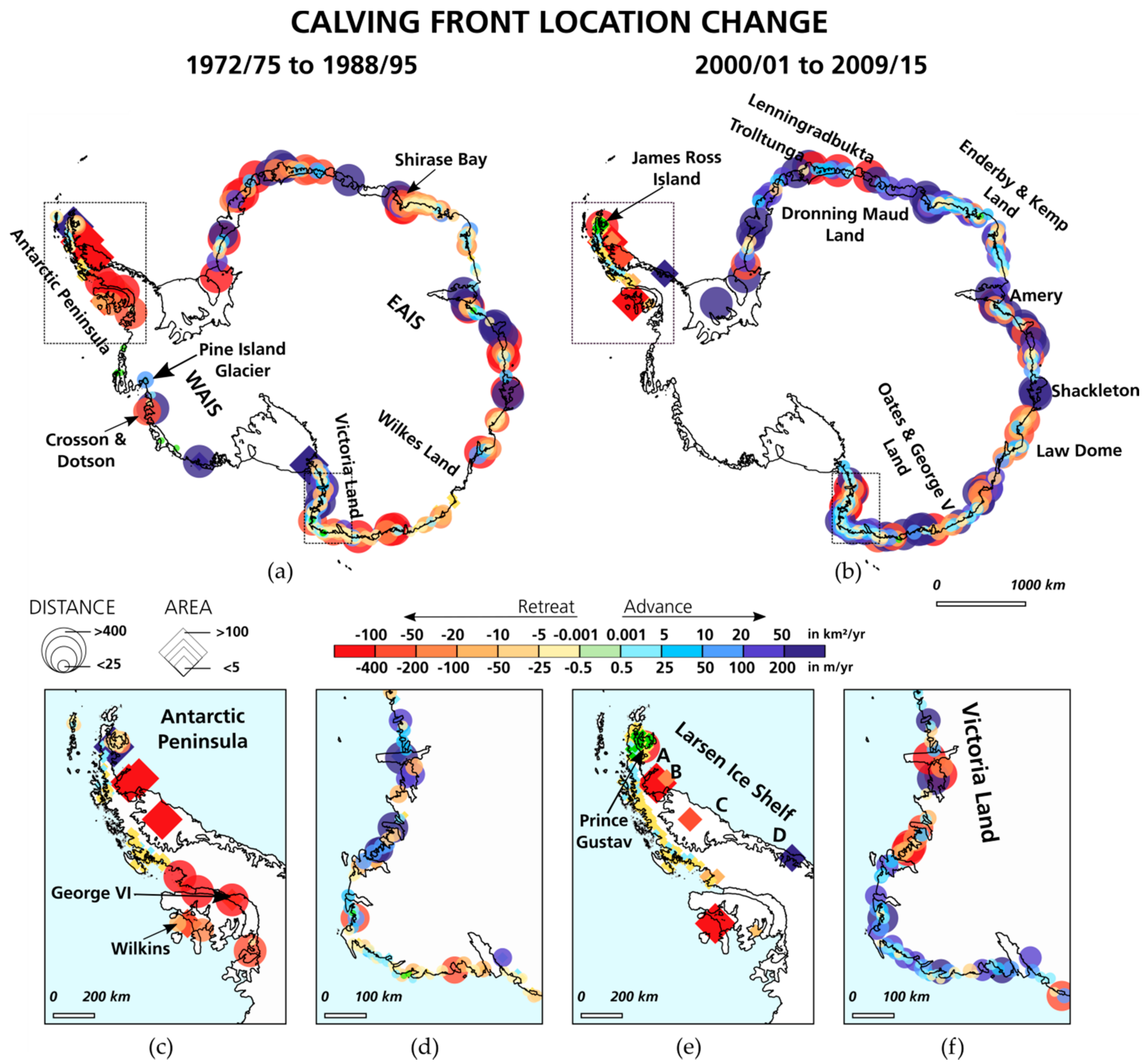
3.7. Circum-Antarctic Calving Front Change Rates

This review also aims to summarize circum-Antarctic patterns of glacier and ice-shelf front changes by combining all of the existing measured CFL. This approach causes various challenges. First of all, data gaps exist for some coastal sections due to a lack of suitable remote sensing imagery. Second, every study measured front stages for different time spans with different intervals. Third, different methods were used to measure front changes. To overcome all of those challenges, some assumptions had to be made. Advance and retreat rates had to be calculated for similar time frames to compare changes in CFL along the Antarctic coastline. To create comparable time periods for each glacier and ice shelf, measured CFL changes from different studies were averaged, as explained in the Supplementary Material, Figure S4 The rates were taken from the reviewed papers in Table S1 in the Supplementary Material. Area and distance measurements were kept separate, as the two cannot be converted without information on glacier width. The annual change rates are averaged for the time frames 1972/75 to 1988/95 and 2000/01 to 2009/15 (detailed calculation is described in the Supplementary Material, Figure S2). Those time frames were chosen to use as many CFL records as possible with large-scale coverage. Assessing circum-Antarctic patterns before 1972 was not possible. No sufficient amounts of East Antarctic CFL records exist before 1972, as Miles et al. (2016) [33] were the first and still only to publish a large-scale calving front study on the EAIS starting in the 1970s. Start and end years vary slightly, depending on available measurements, but do not span more than seven years. Exact start and end points as well as change rates for each measured glacier and ice shelf are available in the Supplementary Excel Sheet.

The results are presented in Figure 7. Advancing and retreating fronts are compared for the periods 1972/75 to 1988/95 and 2000/01 to 2009/15. Circles indicate changes measured by distance, while diamonds indicate changes measured by area. Red colors indicate retreat, whereas blue colors represent advance.

The larger and darker symbols show high annual change rates, and small, light-colored symbols indicate slight changes. For the entire Antarctic coastline, it appears that glacier and ice-shelf front retreat predominates between 1972/75 and 1988/95, and advance occurs between 2000/01 and 2009/15. However, it should be noted that the presented dataset has gaps for some coastal regions, and that measurements locations are not always the same between both timeframes.

Nevertheless, the pattern varies regionally. Glaciers and ice shelves along the Antarctic Peninsula show a retreating trend for both timeframes (Figure 7c,e). Small glaciers along James Ross Island retreated slightly between 1972/75 and 1988/95, except for glaciers terminating into Rhöss Bay. Especially, the huge ice shelves along the Antarctic Peninsula (such as Prince Gustav, Larsen A–C, Wilkins and George VI) show strong retreat rates for the earlier time period. Retreat is still apparent between 2000/01 and 2009/15, but of lower magnitude: Larsen D is the only exception with an advancing front (Figure 7e).

For the WAIS, only measurements for the earlier timeframe are available. During the period 1972/75 to 1988/95, only the Dotson and Crosson ice shelves retreated. The other ice shelves and glaciers advanced or are classified as stable (less than 0.5 m per year). It is important to note that the fronts of West Antarctic ice shelves and glaciers highly fluctuate [30]. This means that a front that is classified as “stable” might have moved within the observation timeframe, and just ended at the same position as it started over the period of observation.

The coastline along the EAIS changed within both observation periods. The glaciers along Victoria Land mostly advanced between 1972/75 and 1988/95, whereas calving fronts along the nearby Oates and George V Land rather retreated (Figure 7d). This tendency reverses between 2000/01 and 2009/15 (Figure 7f). Especially interesting are the strong retreating glaciers along Victoria Land. Investigating changes in boundary conditions and distinguishing between glacier terminus types (e.g., Lovell et al. (2017) [28]) could yield explanations for this change in calving front position. For Wilkes Land, the data availability makes any analysis of coastal change difficult. Slight retreats can be seen for both time periods, but are not comparable, as many measurements are missing between 1972/75 and 1988/95 due to a lack of data. Between the Law Dome site and the Shackleton ice shelves, retreating fronts dominate over the slight advances. Fronts along Enderby and Kemp Land slightly retreated between 1975–1995, but mostly switched to advance in 2000/01 to 2009/15. The same can be observed for the glaciers terminating in the Shirase Glacier Bay, but the magnitude of change is much higher. Dronning Maud Land also shows the tendency of glaciers to retreat during the earlier time frame and advance for the later time frame. Only the ice shelves between Lenningradbukta and Trolltunga still retreated between 2000/01 and 2009/15.

The pattern of circum-Antarctic CFL change can be summarized as follows. In general, the majority of the ice fronts along the Antarctic Peninsula retreated strongly between 1972/75 and 1988/95, and continued to do so between 2000/01 to 2009/15, but with less magnitude. In contrast, most fronts along the WAIS rather advanced between 1972/75 and 1988/95, but it is important to note that only a low amount of records exist, and fronts highly fluctuate in this region, which requires high temporal mapping. For the EAIS, the general trend of retreat between 1972/75 and 1988/95 toward advance between 2000/01 to 2009/15 is apparent. Exceptions of this overall trend are Victoria Land, Wilkes Land, and the northernmost part of Dronning Maud Land.

4. The Future Potential of Earth Observation to Analyze CFLs

The analysis of calving fronts advanced significantly as the number of available satellite products increased. In the future, Earth observation has a high potential to fulfill the needs of calving front mapping of the Antarctic scientific community, as outlined below.

4.1. Need for Homogenized Data

This review presents numerous measurements of CFLs. Nevertheless, the measurements are not always comparable, as different measurement techniques, timespans, and reference areas were used. With increasing volumes of satellite imagery, it becomes more and more important to standardize mapping regarding (i) time periods, (ii) methodology, and (iii) reference areas of glacial features.

The timing of measurements is essential for the definition of retreat and advance. For example, the Amery Ice Shelf showed advance when measured from 1936 to 2010, but retreat when measured from 1963 to 2011. Standardized observation time intervals would allow clear and comparable definitions of retreat and advance. A comparison of glacier change between individual glaciers would be easier and more accurate. Timing also includes the regular monitoring of fronts. For example, trends in East Antarctic calving front changes can only be discovered by the regular observation of CFLs [33]. Earlier studies could not identify those trends, as data availability was restricted, and did not allow monitoring in regular intervals [128]. Besides, a dataset of frequently monitored calving fronts would be a valuable dataset for ice sheet modelers. The so far common but unrealistic flux gate calculations with steady-state fronts [6,52] could finally be replaced by dynamic fronts and improve sea level models significantly [30]. Earth observation can be valuable, as sensors with high repeat rates allow the regular analysis of frontal positions.

A standardized methodology should be based on an automated approach, as the widely used manual delineation of fronts is time-consuming. Automatization would make calving front measurements more comparable, such as the new tool developed by Lea et al. [77]. It is a great support to efficiently extract calving front locations from Landsat and Sentinel satellite imagery, even though manual editing is still necessary. An accurate fully automated algorithm does not yet exist, as it would need to be capable of distinguishing between different backscatter values depending on the season, sea ice conditions, and extract fronts of various morphologies, as shown in Figure 2.

Finally, catchment-based reference areas for glacial features would be important to measure the percentage of change related to glacier size. The absolute retreat rates of glaciers on the Antarctic Peninsula are small compared to the ones of huge ice shelves (e.g., Ronne–Filchner). A specific satellite imagery mosaic (e.g., LIMA) could be used for measuring the initial glacier or ice shelf area and serve as a standard. Additionally, for the future quantification of glacier change, area measurements should be prioritized to capture frontal changes along the entire margin, standardize methodology, and obtain comparable results.

4.2. Need for Longer, More Frequent, and Spatially Complete Measurements

A longer time-series of front fluctuations would be desirable to analyze the impact of changes in air and ocean temperatures on CFLs. Extending the time-series backwards in time with remote sensing is not possible, but nevertheless, already existing imagery and maps could be digitized and measured by a standardized approach, as mentioned above. A good starting point would be the digitalization of the USGS Coastal Change and Glaciological Maps Series of Antarctica. Once the project is finished for the entire continent, a valuable and standardized record of frontal positions would be available. To extend the time-series in the future, abundant data is regularly acquired by Sentinel 1, 2, and 3, Landsat-8, ENVISAT, and MODIS. For the huge amount of data, an automated method for front extraction would be needed. The benefits of high repeat cycles and wide coverage can then be maximized. Additionally, the precision in ice front mapping should be consistent, as the accuracy of early measurements from expeditions (e.g., [109]) differs significantly from the precision of modern measurements based on accurate georeferenced satellite imagery.

4.3. Sensor Requirements

Mapping calving fronts automatically and accurately could be much more efficient with a sensor delivering radar imagery in addition to height information. SAR imagery could be very valuable for the simple reason of independence to illumination and cloud penetration. Additionally, SAR data allows interferometric SAR (InSAR) applications, which have shown potential for coastline extraction [136,137,138]. Sentinel-1 already provides valuable data, but low penetration depth due to the C-band, and the repeat cycle does not always allow coherence between scenes for areas of very dynamic Antarctic glaciers [139]. A higher repeat cycle or even a tandem mission would be needed instead. Additional height information would help with extracting the front more accurately, as the ice front is higher than the water surface. Elevation information can be retrieved either by an altimeter or tandem mission. Up until now, frequent height measurements and an InSAR analysis of the Antarctic coastline would be beyond the power and size of current processing and data storage environments. However, in a time where storage matters less and computing power gets stronger, this kind sensor should be considered.

4.4. Need for Joint Data Analysis

The interest in the Antarctic Ice Sheet is mainly driven by the question of its contribution to sea-level rise [52,140]. To answer this pressing geoscientific question, besides calving fronts, several other parameters need to be jointly assessed. For example, no clear changes in frontal positions could be observed along the WAIS, but many studies confirm high trends in mass loss [6,27,43,44,141]. Therefore, the changes in CFLs should be analyzed in combination with other input data such as elevation data, mass balance estimates, and temperature measurements. The value of a large-scale CFL dataset in combination with environmental variables to explain drivers of glacier change was already presented for Greenland [53,142]. Data on height through altimeters or tandem missions such as TanDEM-X and planned TanDEM-L can offer information on mass loss. Also, the improved version of GRACE (Gravity Recovery and Climate Experiment) - GRACE follow-on - will reveal changes in mass through gravity measurements. Additionally, data on ice-sheet flow velocities [143], warming air temperatures, ocean temperature, and sea-ice extent [144] are other important parameters that are needed to quantify sea-level contribution. It is essential to improve the understanding of iceberg calving and the driving forces behind it [18,46], as well as including dynamic ice shelf and glacier fronts in mass balance calculations [27] and ice sheet models [52]. It is still a long journey to sophisticated ice sheet models, but Earth observation will definitely contribute significantly to offer the best possible input datasets. Only then, models can be calibrated and validated properly and give accurate predictions about future sea level scenarios.

5. Conclusions

This review provides a comprehensive overview of ice shelf and glacier front measurements along the Antarctic coastline. Remote sensing imagery is a valuable resource to measure ice shelf and glacier front dynamics. Optical as well as radar sensors are suitable with individual advantages and drawbacks. In general, both data sources are used to achieve a long-term and spatially as well as temporal denser time-series of front fluctuations. Until now, the favored front extraction method is the manual delineation (used by 85%) from remote sensing imagery, but a trend to pre-classification and manual post-corrections exists. The motivation for CFL studies is either to explain observed ice dynamical changes (45% of studies) or to link changes in the frontal position to climate change and sea-level rise (46%). This reflects the challenge in establishing the influence of climate change on glacier and ice shelf retreat and advance. A uniform circum-Antarctic record on calving front locations will allow a better linkage between changes in boundary conditions and glacier and ice shelf retreat. Sufficient records on calving front studies exist for regions of sensitive marine-terminating outlet glaciers such as the Antarctic Peninsula, South Shetland Islands, and Victoria Land. On the West Antarctic Ice Sheet, only popular individual glaciers and ice shelves (e.g., Pine Island and Thwaites Glacier) are studied frequently. Areal long-term change rates for the WAIS coast and most of the parts of the EAIS are missing. Most of the reviewed studies cover single glacier or ice-shelf fronts (64%), whereas large-scale circum-Antarctic analyses are scarce (9%). Large ice shelves such as Larsen A-D, Wilkins, Filchner-Ronne, and Ross are intensively studied. The temporal availability of calving front measurements varies depending on observation length and intervals. The observation length for the Antarctic Peninsula is mainly between 50–75 years, due to the good coverage of ARGON imagery from the year 1963 and partial coverage of RARE aerial imagery in 1947. Fronts along the EAIS are mapped since the 1970s, except for Wilkes Land. For all of Antarctica, good coverage of recent CFL observations (from 1975 to 2015) exists only for 16% of the total amount of calving fronts that have been mentioned in the reviewed studies. The pattern of glacier change along the Antarctic coastline varies depending on the region and observation period. Calving fronts along the Antarctic Peninsula generally retreated since the 1970s, but with a higher magnitude between 1972–1995 compared to 2000 and 2015. Glaciers and ice shelves are very dynamic along the coastline of the WAIS, where only a small amount of measurements exist. Between 1975–1995, advance dominated. The EAIS shows a general trend of retreating fronts between 1975–1995. In contrast, many of the fronts started to advance between 2000–2015. Exceptions to this trend were identified for Victoria Land, Wilkes Land, and the northernmost part of Dronning Maud Land.

For further analyses, calving front measurements should be extended in space and time where remote sensing data is available. The standardization of observation length, mapping intervals, measurement method, and relative change rates to glacier size are important for comparable analysis. To conclude, standardized and high-interval measurements of calving fronts would revolutionize our understanding of glacier and ice shelf dynamics, contribute to more sophisticated ice sheet models by replacing steady-state calving front assumptions, and allow a better identification of the boundary conditions driving calving front changes.

References

1. Swithinbank, C.; Chinn, T.J.; Williams, R.S.; Ferrigno, J.G. Satellite Image Atlas of Glaciers of the World: Antarctica; U.S. Geological Survey Professional Paper 1386-B; United States Government Printing Office: Washington, DC, USA, 1988. [Google Scholar]
2. Fox, A.J.; Cooper, R. Measured properties of the Antarctic ice sheet derived from the SCAR Antarctic digital database. Polar Record 1994, 30, 201–206. [Google Scholar] [CrossRef]
3. Vaughan, D.G.; Comiso, J.C.; Allison, I.; Carrasco, J.; Kaser, G.; Kwok, R.; Mote, P.; Murray, T.; Paul, F.; Ren, J.; et al. Observations: Cryosphere. Clim. Chang. 2013, 2103, 317–382. [Google Scholar]
4. IMBIE. Mass balance of the Antarctic Ice Sheet from 1992 to 2017. Nature 2018, 558, 219–222. [Google Scholar] [CrossRef] [PubMed]
5. Liu, H.; Jezek, K.C. Automated extraction of coastline from satellite imagery by integrating Canny edge detection and locally adaptive thresholding methods. Int. J. Remote Sens. 2004, 25, 937–958. [Google Scholar] [CrossRef]
6. Rignot, E.; Jacobs, S.; Mouginot, J.; Scheuchl, B. Ice-shelf melting around Antarctica. Science 2013, 341, 266–270. [Google Scholar] [CrossRef] [PubMed]
7. Radić, V.; Bliss, A.; Beedlow, A.C.; Hock, R.; Miles, E.; Cogley, J.G. Regional and global projections of twenty-first century glacier mass changes in response to climate scenarios from global climate models. Clim. Dyn. 2014, 42, 37–58. [Google Scholar] [CrossRef]
8. Rose, G.; McElroy, C.T. Coal Potential of Antarctica; Australia Bureau of Mineral Resources, Geology and Geophysics; Australian Government Publishing Service: Canberra, Australia, 1987.
9. Wright, N.A.; Williams, P.L. Mineral Resources of Antarctica; United States Department of the Interior: Washington, DC, USA, 1974. [Google Scholar]
10. Naylor, S.; Siegert, M.; Dean, K.; Turchetti, S. Science, geopolitics and the governance of Antarctica. Nat. Geosci. 2008, 1, 143–143. [Google Scholar] [CrossRef]
11. Secretariat of the Antarctic Treaty. Compilation of Key Documents of the Antarctic Treaty System, 3rd ed.; Secretariat of the Antarctic Treaty: Buenos Aires, Argentina, 2017; Volume 3. [Google Scholar]
12. Swithinbank, C. Airborne tourism in the Antarctic. Polar Record 1993, 29, 103–110. [Google Scholar] [CrossRef]
13. Dodds, K. Governing Antarctica: Contemporary Challenges and the Enduring Legacy of the 1959 Antarctic Treaty. Glob. Policy 2010, 1, 108–115. [Google Scholar] [CrossRef] [Green Version]
14. Bindoff, N.L.; Stott, P.A.; AchutaRao, K.M.; Allen, M.R.; Gillett, N.; Gutzler, D.; Hansingo, K.; Hegerl, G.; Hu, Y.; Jain, S.; et al. Detection and Attribution of Climate Change: From Global to Regional. In Climate Change 2013: The Physical Science Basis; Contribution of Working Group I to the Fifth Assessment Report of the Intergovernmental Panel on Climate, Change; Stocker, T.F., Qin, D., Plattner, G.-K., Tignor, M., Allen, S.K., Boschung, J., Nauels, A., Xia, Y., Bex, V., Midgley, P.M., Eds.; Cambridge University Press: Cambridge, UK; New York, NY, USA, 2013. [Google Scholar]
15. Miles, B. Synchronous Terminus Change of East Antarctic Outlet Glaciers Linked to Climatic Forcing. Master’s Thesis, Durham University, Durham, UK, 2013. [Google Scholar]
16. Foga, S.; Stearns, L.A.; Van der Veen, C.J. Application of satellite remote sensing techniques to quantify terminus and ice mélange behavior at Helheim Glacier, East Greenland. Mar. Technol. Soc. J. 2014, 48, 81–91. [Google Scholar] [CrossRef]
17. Benn, D.I.; Warren, C.R.; Mottram, R.H. Calving processes and the dynamics of calving glaciers. Earth-Sci. Rev. 2007, 82, 143–179. [Google Scholar] [CrossRef]
18. Luckman, A.; Benn, D.I.; Cottier, F.; Bevan, S.; Nilsen, F.; Inall, M. Calving rates at tidewater glaciers vary strongly with ocean temperature. Nat. Commun. 2015, 6, 8566. [Google Scholar] [CrossRef] [PubMed] [Green Version]
19. Bindschadler, R.A. History of lower Pine Island Glacier, West Antarctica, from Landsat imagery. J. Glaciol. 2002, 48, 536–544. [Google Scholar] [CrossRef]
20. Massom, R.A.; Giles, A.B.; Warner, R.C.; Fricker, H.A.; Legresy, B.; Hyland, G.; Lescarmontier, L.; Young, N. External influences on the Mertz Glacier Tongue (East Antarctica) in the decade leading up to its calving in 2010. J. Geophys. Res.-Earth Surf. 2015, 120, 490–506. [Google Scholar] [CrossRef] [Green Version]
21. Rott, H.; Rack, W.; Skvarca, P.; De Angelis, H. Northern Larsen ice shelf, Antarctica: Further retreat after collapse. Ann. Glaciol. 2002, 34, 277–282. [Google Scholar] [CrossRef]
22. Fountain, A.G.; Glenn, B.; Scambos, T.A. The changing extent of the glaciers along the western Ross Sea, Antarctica. Geology 2017, 45, 927–930. [Google Scholar] [CrossRef]
23. Cook, A.J.; Vaughan, D.G. Overview of areal changes of the ice shelves on the Antarctic Peninsula over the past 50 years. Cryosphere 2010, 4, 77–98. [Google Scholar] [CrossRef] [Green Version]
24. Cook, A.J.; Fox, A.J.; Vaughan, D.G.; Ferrigno, J.G. Retreating glacier fronts on the Antarctic Peninsula over the past half-century. Science 2005, 308, 541–544. [Google Scholar] [CrossRef] [PubMed]
25. Scambos, T.A.; Haran, T.M.; Fahnestock, M.A.; Painter, T.H.; Bohlander, J. MODIS-based Mosaic of Antarctica (MOA) data sets: Continent-wide surface morphology and snow grain size. Remote Sens. Environ. 2007, 111, 242–257. [Google Scholar] [CrossRef]
26. Liu, H.; Jezek, K.C. A complete high-resolution coastline of Antarctica extracted from orthorectified Radarsat SAR imagery. Photogramm. Eng. Remote Sens. 2004, 70, 605–616. [Google Scholar] [CrossRef]
27. Liu, Y.; Moore, J.C.; Cheng, X.; Gladstone, R.M.; Bassis, J.N.; Liu, H.; Wen, J.; Hui, F. Ocean-driven thinning enhances iceberg calving and retreat of Antarctic ice shelves. Proc. Natl. Acad. Sci. USA 2015, 112, 3263–3268. [Google Scholar] [CrossRef] [PubMed] [Green Version]
28. Lovell, A.M.; Stokes, C.R.; Jamieson, S.S.R. Sub-decadal variations in outlet glacier terminus positions in Victoria Land, Oates Land and George V Land, East Antarctica (1972–2013). Antarct. Sci. 2017, 29, 468–483. [Google Scholar] [CrossRef]
29. Cook, A.J.; Holland, P.R.; Meredith, M.P.; Murray, T.; Luckman, A.; Vaughan, D.G. Ocean forcing of glacier retreat in the western Antarctic Peninsula. Science 2016, 353, 283–286. [Google Scholar] [CrossRef] [PubMed] [Green Version]
30. MacGregor, J.A.; Catania, G.A.; Markowski, M.S.; Andrews, A.G. Widespread rifting and retreat of ice-shelf margins in the eastern Amundsen Sea Embayment between 1972 and 2011. J. Glaciol. 2012, 58, 458–466. [Google Scholar] [CrossRef]
31. Nicholls, K.W.; Østerhus, S.; Makinson, K.; Gammelsrød, T.; Fahrbach, E. Ice-ocean processes over the continental shelf of the southern Weddell Sea, Antarctica: A review. Rev. Geophys. 2009, 47, RG3003. [Google Scholar] [CrossRef]
32. Bindschadler, R. Monitoring ice sheet behavior from space. Rev. Geophys. 1998, 36, 79–104. [Google Scholar] [CrossRef] [Green Version]
33. Miles, B.W.J.; Stokes, C.R.; Jamieson, S.S.R. Pan–ice-sheet glacier terminus change in East Antarctica reveals sensitivity of Wilkes Land to sea-ice changes. Sci. Adv. 2016, 2, e1501350. [Google Scholar] [CrossRef] [PubMed] [Green Version]
34. Bassis, J.N. The statistical physics of iceberg calving and the emergence of universal calving laws. J. Glaciol. 2011, 57, 3–16. [Google Scholar] [CrossRef] [Green Version]
35. Wesche, C.; Jansen, D.; Dierking, W. Calving Fronts of Antarctica: Mapping and Classification. Remote Sens. 2013, 5, 6305–6322. [Google Scholar] [CrossRef] [Green Version]
36. Zwally, H.J.; Beckley, M.A.; Brenner, A.C.; Giovinetto, M.B. Motion of major ice-shelf fronts in Antarctica from slant-range analysis of radar altimeter data, 1978–1998. Ann. Glaciol. 2002, 34, 255–262. [Google Scholar] [CrossRef]
37. Urbanski, J.A. A GIS tool for two-dimensional glacier-terminus change tracking. Comput. Geosci. 2018, 111, 97–104. [Google Scholar] [CrossRef]
38. Frezzotti, M.; Polizzi, M. 50 years of ice-front changes between the Adélie and Banzare Coasts, East Antarctica. Ann. Glaciol. 2002, 34, 235–240. [Google Scholar] [CrossRef]
39. Ferrigno, J.G.; Williams Jr, R.S.; Rosanova, C.E.; Lucciiitta, B.K.; Swithinbank, C. Analysis of coastal change in Marie Byrd Land and Ellsworth Land, West Antarctica, using Landsat imagery. Ann. Glaciol. 1998, 27, 33–40. [Google Scholar] [CrossRef] [Green Version]
40. Williams, R.S.; Ferrigno, J.G.; Swithinbank, C.; Lucchitta, B.K.; Seekins, B.A. Coastal-change and glaciological maps of Antarctica. Ann. Glaciol. 1995, 21, 284–290. [Google Scholar] [CrossRef] [Green Version]
41. Pollard, D.; DeConto, R.M.; Alley, R.B. Potential Antarctic Ice Sheet retreat driven by hydrofracturing and ice cliff failure. Earth Planet. Sci. Lett. 2015, 412, 112–121. [Google Scholar] [CrossRef]
42. Hindmarsh, R.C.A. An observationally validated theory of viscous flow dynamics at the ice-shelf calving front. J. Glaciol. 2012, 58, 375–387. [Google Scholar] [CrossRef] [Green Version]
43. Depoorter, M.A.; Bamber, J.L.; Griggs, J.A.; Lenaerts, J.T.M.; Ligtenberg, S.R.M.; Van den Broeke, M.R.; Moholdt, G. Calving fluxes and basal melt rates of Antarctic ice shelves. Nature 2013, 502, 89. [Google Scholar] [CrossRef] [PubMed]
44. Paolo, F.S.; Fricker, H.A.; Padman, L. Volume loss from Antarctic ice shelves is accelerating. Science 2015, 348, 327–331. [Google Scholar] [CrossRef] [PubMed]
45. Hanna, E.; Navarro, F.J.; Pattyn, F.; Domingues, C.M.; Fettweis, X.; Ivins, E.R.; Nicholls, R.J.; Ritz, C.; Smith, B.; Tulaczyk, S.; et al. Ice-sheet mass balance and climate change. Nature 2013, 498, 51–59. [Google Scholar] [CrossRef] [PubMed] [Green Version]
46. Miles, B.W.J.; Stokes, C.R.; Jamieson, S.S.R. Simultaneous disintegration of outlet glaciers in Porpoise Bay (Wilkes Land), East Antarctica, driven by sea ice break-up. Cryosphere 2017, 11, 427–442. [Google Scholar] [CrossRef] [Green Version]
47. Fricker, H.A.; Young, N.W.; Allison, I.; Coleman, R. Iceberg calving from the Amery Ice Shelf, East Antarctica. Ann. Glaciol. 2002, 34, 241–246. [Google Scholar] [CrossRef]
48. Friedl, P.; Seehaus, T.C.; Wendt, A.; Braun, M.H.; Höppner, K. Recent dynamic changes on Fleming Glacier after the disintegration of Wordie Ice Shelf, Antarctic Peninsula. Cryosphere 2018, 12, 1347–1365. [Google Scholar] [CrossRef]
49. Alley, R.B.; Anandakrishnan, S.; Christianson, K.; Horgan, H.J.; Muto, A.; Parizek, B.R.; Pollard, D.; Walker, R.T. Oceanic forcing of ice-sheet retreat: West Antarctica and more. Annu. Rev. Earth Planet. Sci. 2015, 43, 207–231. [Google Scholar] [CrossRef]
50. Rignot, E.; Casassa, G.; Gogineni, P.; Krabill, W.; Rivera, A.; Thomas, R. Accelerated ice discharge from the Antarctic Peninsula following the collapse of Larsen B ice shelf. Geophys. Res. Lett. 2004, 31. [Google Scholar] [CrossRef] [Green Version]
51. Hill, E.A.; Carr, J.R.; Stokes, C.R.; Gudmundsson, G.H. Dynamic changes in outlet glaciers in northern Greenland from 1948 to 2015. Cryosphere Discuss. 2018. [Google Scholar] [CrossRef]
52. DeConto, R.M.; Pollard, D. Contribution of Antarctica to past and future sea-level rise. Nature 2016, 531, 591–597. [Google Scholar] [CrossRef] [PubMed]
53. Moon, T.; Joughin, I. Changes in ice front position on Greenland’s outlet glaciers from 1992 to 2007. J. Geophys. Res. Earth Surf. 2008, 113. [Google Scholar] [CrossRef]
54. Seale, A.; Christoffersen, P.; Mugford, R.I.; O’Leary, M. Ocean forcing of the Greenland Ice Sheet: Calving fronts and patterns of retreat identified by automatic satellite monitoring of eastern outlet glaciers. J. Geophys. Res. Earth Surf. 2011, 116. [Google Scholar] [CrossRef] [Green Version]
55. Bamber, J.L.; Rivera, A. A review of remote sensing methods for glacier mass balance determination. Glob. Planet. Chang. 2007, 59, 138–148. [Google Scholar] [CrossRef]
56. Nick, F.M.; Vieli, A.; Howat, I.M.; Joughin, I. Large-scale changes in Greenland outlet glacier dynamics triggered at the terminus. Nat. Geosci. 2009, 2, 110–114. [Google Scholar] [CrossRef]
57. Liu, H.; Wang, L.; Jezek, K.C. Automated delineation of dry and melt snow zones in Antarctica using active and passive microwave observations from space. IEEE Trans. Geosci. Remote Sens. 2006, 44, 2152–2163. [Google Scholar]
58. Fahnestock, M.; Bindschadler, R.; Kwok, R.; Jezek, K. Greenland ice sheet surface properties and ice dynamics from ERS-1 SAR imagery. Science 1993, 262, 1530–1530. [Google Scholar] [CrossRef] [PubMed]
59. Kwok, R.; Rignot, E.; Holt, B.; Onstott, R. Identification of sea ice types in spaceborne synthetic aperture radar data. J. Geophys. Res. Oceans 1992, 97, 2391–2402. [Google Scholar] [CrossRef] [Green Version]
60. Bogdanov, A.V.; Sandven, S.; Johannessen, O.M.; Alexandrov, V.Y.; Bobylev, L.P. Multisensor approach to automated classification of sea ice image data. IEEE Trans. Geosci. Remote Sens. 2005, 43, 1648–1664. [Google Scholar] [CrossRef] [Green Version]
61. Ressel, R.; Frost, A.; Lehner, S. Comparing automated sea ice classification on single-pol and dual-pol TerraSAR-X data. In Proceedings of the 2015 IEEE International Geoscience and Remote Sensing Symposium (IGARSS), Milan, Italy, 26–31 July 2015; pp. 3442–3445. [Google Scholar]
62. Wesche, C.; Dierking, W. Iceberg signatures and detection in SAR images in two test regions of the Weddell Sea, Antarctica. J. Glaciol. 2012, 58, 325–339. [Google Scholar] [CrossRef] [Green Version]
63. König, M.; Winther, J.-G.; Isaksson, E. Measuring snow and glacier ice properties from satellite. Rev. Geophys. 2001, 39, 1–27. [Google Scholar] [CrossRef] [Green Version]
64. Dietz, A.J.; Kuenzer, C.; Gessner, U.; Dech, S. Remote sensing of snow—A review of available methods. Int. J. Remote Sens. 2012, 33, 4094–4134. [Google Scholar] [CrossRef]
65. Klinger, T.; Ziems, M.; Heipke, C.; Schenke, H.W.; Ott, N. Antarctic Coastline Detection using Snakes. Photogramm. Fernerkund. Geoinf. 2011, 2011, 421–434. [Google Scholar] [CrossRef]
66. Partington, K.C. Discrimination of glacier facies using multi-temporal SAR data. J. Glaciol. 1998, 44, 41–53. [Google Scholar] [CrossRef]
67. Tedesco, M. Remote Sensing of the Cryosphere; John Wiley & Sons: Hoboken, NJ, USA, 2014. [Google Scholar]
68. Gao, B.-C.; Han, W.; Tsay, S.C.; Larsen, N.F. Cloud detection over the Arctic region using airborne imaging spectrometer data during the daytime. J. Appl. Meteorol. 1998, 37, 1421–1429. [Google Scholar] [CrossRef]
69. Zeng, Q.; Cao, M.; Feng, X.; Liang, F.; Chen, X.; Sheng, W. A study of spectral reflection characteristics for snow, ice and water in the north of China. Hydrol. Appl. Remote Sens. Remote Data Transm. 1984, 145, 451–462. [Google Scholar]
70. Rau, F.; Mauz, F.; De Angelis, H.; Jaña, R.; Neto, J.A.; Skvarca, P.; Vogt, S.; Saurer, H.; Gossmann, H. Variations of glacier frontal positions on the northern Antarctic Peninsula. Ann. Glaciol. 2004, 39, 525–530. [Google Scholar] [CrossRef]
71. Mason, D.C.; Davenport, I.J. Accurate and efficient determination of the shoreline in ERS-1 SAR images. IEEE Trans. Geosci. Remote Sens. 1996, 34, 1243–1253. [Google Scholar] [CrossRef]
72. Caspar, C.; Colin, O.; Laur, H.; Tell, B.R.; Mathot, E.; Tandurella, G.; Goncalves, P.; Brito, F. Generation of ENVISAT ASAR mosaics accessible on-line. In Proceedings of the IEEE International Geoscience and Remote Sensing Symposium, Barcelona, Spain, 23–28 July 2007; pp. 1405–1408. [Google Scholar]
73. Kuenzer, C.; Ottinger, M.; Wegmann, M.; Guo, H.; Wang, C.; Zhang, J.; Dech, S.; Wikelski, M. Earth observation satellite sensors for biodiversity monitoring: Potentials and bottlenecks. Int. J. Remote Sens. 2014, 35, 6599–6647. [Google Scholar] [CrossRef]
74. Kim, K.; Jezek, K.C.; Liu, H. Orthorectified image mosaic of Antarctica from 1963 Argon satellite photography: Image processing and glaciological applications. Int. J. Remote Sens. 2007, 28, 5357–5373. [Google Scholar] [CrossRef]
75. Lee, J.; Jurkevich, I. Coastline Detection and Tracing InSAR Images. IEEE Trans. Geosci. Remote Sens. 1990, 28, 662–668. [Google Scholar] [CrossRef]
76. Wu, S.Y.; Liu, A.K. Towards an automated ocean feature detection, extraction and classification scheme for SAR imagery. Int. J. Remote Sens. 2003, 24, 935–951. [Google Scholar] [CrossRef]
77. Lea, J.M. Google Earth Engine Digitisation Tool (GEEDiT), and Margin change Quantification Tool (MaQiT)—Simple tools for the rapid mapping and quantification of changing Earth surface margins. Earth Surf. Dyn. Discuss. 2018, 6, 551–561. [Google Scholar] [CrossRef]
78. Sohn, H.-G.; Jezek, K.C. Mapping ice sheet margins from ERS-1 SAR and SPOT imagery. Int. J. Remote Sens. 1999, 20, 3201–3216. [Google Scholar] [CrossRef]
79. Krieger, L.; Floricioiu, D. Automatic calving front delienation on TerraSAR-X and Sentinel-1 SAR imagery. In Proceedings of the IEEE International Geoscience and Remote Sensing Symposium (IGARSS), Fort Worth, TX, USA, 23–28 July 2017. [Google Scholar]
80. Lea, J.M.; Mair, D.W.F.; Rea, B.R. Evaluation of existing and new methods of tracking glacier terminus change. J. Glaciol. 2014, 60, 323–332. [Google Scholar] [CrossRef] [Green Version]
81. Skvarca, P.; Rack, W.; Rott, H.; Donángelo, T.I. Climatic trend and the retreat and disintegration of ice shelves on the Antarctic Peninsula: An overview. Polar Res. 1999, 18, 151–157. [Google Scholar] [CrossRef]
82. Bevan, S.L.; Luckman, A.J.; Murray, T. Glacier dynamics over the last quarter of a century at Helheim, Kangerdlugssuaq and 14 other major Greenland outlet glaciers. Cryosphere 2012, 6, 923–937. [Google Scholar] [CrossRef] [Green Version]
83. Ferrigno, J.G.; Cook, A.J.; Foley, K.M.; Williams, R.S.; Swithinbank, C.; Fox, A.J.; Thomson, J.W.; Sievers, J. Coastal-Change and Glaciological Map of the Trinity Peninsula area and South Shetland Islands, Antarctica: 1843–2001; USGS Geologic Investigation Series; U.S. Geological Survey: Reston, VA, USA, 2006. [Google Scholar]
84. Fukuda, T.; Sugiyama, S.; Sawagaki, T.; Nakamura, K. Recent variations in the terminus position, ice velocity and surface elevation of Langhovde Glacier, East Antarctica. Antarct. Sci. 2014, 26, 636–645. [Google Scholar] [CrossRef] [Green Version]
85. Davies, B.J.; Carrivick, J.L.; Glasser, N.F.; Hambrey, M.J.; Smellie, J.L. Variable glacier response to atmospheric warming, northern Antarctic Peninsula, 1988–2009. Cryosphere 2012, 6, 1031–1048. [Google Scholar] [CrossRef] [Green Version]
86. Cook, A.J.; Vaughan, D.G.; Luckman, A.J.; Murray, T. A new Antarctic Peninsula glacier basin inventory and observed area changes since the 1940s. Antarct. Sci. 2014, 26, 614–624. [Google Scholar] [CrossRef] [Green Version]
87. Kim, K.T.; Jezek, K.C.; Sohn, H.G. Ice shelf advance and retreat rates along the coast of Queen Maud Land, Antarctica. J. Geophys. Res. Oceans 2001, 106, 7097–7106. [Google Scholar] [CrossRef] [Green Version]
88. Anderson, R.; Jones, D.H.; Gudmundsson, G.H. Halley Research Station, Antarctica: Calving risks and monitoring strategies. Nat. Hazards Earth Syst. Sci. 2014, 14, 917–927. [Google Scholar] [CrossRef] [Green Version]
89. Sahade, R.; Lagger, C.; Torre, L.; Momo, F.; Monien, P.; Schloss, I.; Barnes, D.K.A.; Servetto, N.; Tarantelli, S.; Tatián, M.; et al. Climate change and glacier retreat drive shifts in an Antarctic benthic ecosystem. Sci. Adv. 2015, 1, e1500050. [Google Scholar] [CrossRef] [PubMed] [Green Version]
90. Peck, L.S.; Barnes, D.K.A.; Cook, A.J.; Fleming, A.H.; Clarke, A. Negative feedback in the cold: Ice retreat produces new carbon sinks in Antarctica. Glob. Chang. Biol. 2010, 16, 2614–2623. [Google Scholar] [CrossRef]
91. Bindschadler, R.; Vornberger, P.; Fleming, A.; Fox, A.; Mullins, J.; Binnie, D.; Paulsen, S.J.; Granneman, B.; Gorodetzky, D. The Landsat image mosaic of Antarctica. Remote Sens. Environ. 2008, 112, 4214–4226. [Google Scholar] [CrossRef]
92. Kunz, M.; Mills, J.P.; Miller, P.E.; King, M.A.; Fox, A.J.; Marsh, S. Application of surface matching for improved measurements of historic glacier volume change in the Antarctic Peninsula. Int. Arch. Photogramm. Remote Sens. Spat. Inform. Sci. 2012, 39, 579–584. [Google Scholar] [CrossRef]
93. Ward, C.G. Mapping ice front changes of Müller Ice Shelf, Antarctic Peninsula. Antarct. Sci. 1995, 7, 197–198. [Google Scholar] [CrossRef]
94. Albrecht, T.; Levermann, A. Spontaneous ice-front retreat caused by disintegration of adjacent ice shelf in Antarctica. Earth Planet. Sci. Lett. 2014, 393, 26–30. [Google Scholar] [CrossRef]
95. Massom, R.A.; Scambos, T.A.; Bennetts, L.G.; Reid, P.; Squire, V.A.; Stammerjohn, S.E. Antarctic ice shelf disintegration triggered by sea ice loss and ocean swell. Nature 2018, 558, 383–389. [Google Scholar] [CrossRef] [PubMed]
96. Schodlok, M.P.; Menemenlis, D.; Rignot, E.J. Ice shelf basal melt rates around Antarctica from simulations and observations. J. Geophys. Res. Oceans 2016, 121, 1085–1109. [Google Scholar] [CrossRef] [Green Version]
97. Khazendar, A.; Borstad, C.P.; Scheuchl, B.; Rignot, E.; Seroussi, H. The evolving instability of the remnant Larsen B Ice Shelf and its tributary glaciers. Earth Planet. Sci. Lett. 2015, 419, 199–210. [Google Scholar] [CrossRef] [Green Version]
98. Pritchard, Hd.; Ligtenberg, S.R.M.; Fricker, H.A.; Vaughan, D.G.; Van den Broeke, M.R.; Padman, L. Antarctic ice-sheet loss driven by basal melting of ice shelves. Nature 2012, 484, 502–505. [Google Scholar] [CrossRef] [PubMed]
99. Lee, J.; Jin, Y.K.; Hong, J.K.; Yoo, H.J.; Shon, H. Simulation of a tidewater glacier evolution in Marian Cove, King George Island, Antarctica. Geosci. J. 2008, 12, 33–39. [Google Scholar] [CrossRef]
100. Rückamp, M.; Braun, M.; Suckro, S.; Blindow, N. Observed glacial changes on the King George Island ice cap, Antarctica, in the last decade. Glob. Planet. Chang. 2011, 79, 99–109. [Google Scholar] [CrossRef]
101. Simões, J.C.; Bremer, U.F.; Aquino, F.E.; Ferron, F.A. Morphology and variations of glacial drainage basins in the King George Island ice field, Antarctica. Ann. Glaciol. 1999, 29, 220–224. [Google Scholar] [CrossRef] [Green Version]
102. Skvarca, P. Changes and surface features of the Larsen Ice Shelf, Antarctica, derived from Landsat and Kosmos mosaics. Ann. Glaciol. 1994, 20, 6–12. [Google Scholar] [CrossRef]
103. Rott, H.; Skvarca, P.; Nagler, T. Rapid collapse of northern Larsen Ice Shelf, Antarctica. Science 1996, 271, 788–792. [Google Scholar] [CrossRef]
104. Scambos, T.A.; Bohlander, J.A.; Shuman, C.A.; Skvarca, P. Glacier acceleration and thinning after ice shelf collapse in the Larsen B embayment, Antarctica. Geophys. Res. Lett. 2004, 31. [Google Scholar] [CrossRef] [Green Version]
105. Glasser, N.F.; Kulessa, B.; Luckman, A.; Jansen, D.; King, E.C.; Sammonds, P.R.; Scambos, T.A.; Jezek, K.C. Surface structure and stability of the Larsen C ice shelf, Antarctic Peninsula. J. Glaciol. 2009, 55, 400–410. [Google Scholar] [CrossRef] [Green Version]
106. Rankl, M.; Fürst, J.J.; Humbert, A.; Braun, M.H. Dynamic changes on the Wilkins Ice Shelf during the 2006--2009 retreat derived from satellite observations. Cryosphere 2017, 11, 1199–1211. [Google Scholar] [CrossRef]
107. Braun, M.; Humbert, A.; Moll, A. Changes of Wilkins Ice Shelf over the past 15 years and inferences on its stability. Cryosphere 2009, 3, 41–56. [Google Scholar] [CrossRef] [Green Version]
108. Arigony-Neto, J.; Skvarca, P.; Marinsek, S.; Braun, M.; Humbert, A.; Júnior, C.W.M.; Jaña, R. Monitoring glacier changes on the Antarctic Peninsula. In Global Land Ice Measurements from Space; Springer: Berlin, Germany, 2014; pp. 717–741. [Google Scholar]
109. Ross, J.C. A Voyage of Discovery and Research in the Southern and Antarctic Regions, during the Years 1839-43; John Murray: London, UK, 1847; Volume 1. [Google Scholar]
110. Keys, H.J.R.; Jacobs, S.S.; Brigham, L.W. Continued northward expansion of the Ross Ice Shelf, Antarctica. Ann. Glaciol. 1998, 27, 93–98. [Google Scholar] [CrossRef] [Green Version]
111. Jacobs, S. The Voyage of Iceberg B-9. Am. Sci. 1992, 80, 32–42. [Google Scholar]
112. Rignot, E. Ice-shelf changes in Pine Island Bay, Antarctica, 1947–2000. J. Glaciol. 2002, 48, 247–256. [Google Scholar] [CrossRef]
113. Jenkins, A.; Vaughan, D.G.; Jacobs, S.S.; Hellmer, H.H.; Keys, J.R. Glaciological and oceanographic evidence of high melt rates beneath Pine Island Glacier, West Antarctica. J. Glaciol. 1997, 43, 114–121. [Google Scholar] [CrossRef]
114. Jenkins, A.; Dutrieux, P.; Jacobs, S.S.; McPhail, S.D.; Perrett, J.R.; Webb, A.T.; White, D. Observations beneath Pine Island Glacier in West Antarctica and implications for its retreat. Nat. Geosci. 2010, 3, 468–472. [Google Scholar] [CrossRef] [Green Version]
115. Dutrieux, P.; Vaughan, D.G.; Corr, H.F.J.; Jenkins, A.; Holland, P.R.; Joughin, I.; Fleming, A.H. Pine Island glacier ice shelf melt distributed at kilometre scales. Cryosphere 2013, 7, 1543–1555. [Google Scholar] [CrossRef] [Green Version]
116. Shepherd, A.; Wingham, D.J.; Mansley, J.A.D.; Corr, H.F.J. Inland thinning of pine island Glacier, West Antarctica. Science 2001, 291, 862–864. [Google Scholar] [CrossRef] [PubMed]
117. Jacobs, S.S.; Jenkins, A.; Giulivi, C.F.; Dutrieux, P. Stronger ocean circulation and increased melting under Pine Island Glacier ice shelf. Nat. Geosci. 2011, 4, 519–523. [Google Scholar] [CrossRef] [Green Version]
118. Wendler, G.; Ahlnäs, K.; Lingle, C.S. On Mertz and Ninnis Glaciers, East Antarctica. J. Glaciol. 1996, 42, 447–453. [Google Scholar] [CrossRef] [Green Version]
119. Wang, X.; Holland, D.M.; Cheng, X.; Gong, P. Grounding and calving cycle of Mertz Ice Tongue revealed by shallow Mertz Bank. Cryosphere 2016, 10, 2043–2056. [Google Scholar] [CrossRef]
120. Giles, A.B. The Mertz Glacier Tongue, East Antarctica. Changes in the past 100 years and its cyclic nature - Past, present and future. Remote Sens. Environ. 2017, 191, 30–37. [Google Scholar] [CrossRef]
121. Walker, C.C.; Bassis, J.N.; Fricker, H.A.; Czerwinski, R.J. Observations of interannual and spatial variability in rift propagation in the Amery Ice Shelf, Antarctica, 2002–14. J. Glaciol. 2015, 61, 243–252. [Google Scholar] [CrossRef] [Green Version]
122. Huber, J.; Cook, A.J.; Paul, F.; Zemp, M. A complete glacier inventory of the Antarctic Peninsula based on Landsat 7 images from 2000 to 2002 and other preexisting data sets. Earth Syst. Sci. Data 2017, 9, 115–131. [Google Scholar] [CrossRef]
123. Holt, T.O.; Glasser, N.F.; Quincey, D.J.; Siegfried, M.R. Speedup and fracturing of George VI Ice Shelf, Antarctic Peninsula. Cryosphere 2013, 7, 373–417. [Google Scholar] [CrossRef] [Green Version]
124. Doake, C.S.M.; Corr, H.F.J.; Rott, H.; Skvarca, P.; Young, N.W. Breakup and conditions for stability of the northern Larsen Ice Shelf, Antarctica. Nature 1998, 391, 778–780. [Google Scholar] [CrossRef]
125. Glasser, N.F.; Scambos, T.A.; Bohlander, J.; Truffer, M.; Pettit, E.; Davies, B.J. From ice-shelf tributary to tidewater glacier: Continued rapid recession, acceleration and thinning of Rohss Glacier following the 1995 collapse of the Prince Gustav Ice Shelf, Antarctic Peninsula. J. Glaciol. 2011, 57, 397–406. [Google Scholar] [CrossRef]
126. Ferrigno, J.G.; Williams, R.S.; Foley, K.M. Coastal-Change and Glaciological Map of the Saunders Coast Area, Antarctica: 1972–97. Ann. Glaciol. 2005, 39, 245–250. [Google Scholar] [CrossRef]
127. Frezzotti, M.; Gimbelli, A.; Ferrigno, J.G. Ice-front change and iceberg behaviour along Oates and George V Coasts, Antarctica, 1912–96. Ann. Glaciol. 1998, 27, 643–650. [Google Scholar] [CrossRef]
128. Frezzotti, M. Ice front fluctuation, iceberg calving flux and mass balance of Victoria Land glaciers. Antarct. Sci. 1997, 9, 61–73. [Google Scholar] [CrossRef]
129. Swithinbank, C.; Williams, R.S., Jr.; Ferrigno, J.G.; Seekins, B.A.; Lucchita, B.K.; Rosanova, C.E. Coastal-Change and Glaciological Map of the Bakutis Coast, Antarctica; IMAP: Reston, VA, USA, 1997. [Google Scholar]
130. Jezek, K.C. RADARSAT-1 Antarctic Mapping Project: Change-detection and surface velocity campaign. Ann. Glaciol. 2002, 34, 263–268. [Google Scholar] [CrossRef]
131. Pope, A.; Rees, W.G.; Fox, A.J.; Fleming, A. Open access data in polar and cryospheric remote sensing. Remote Sens. 2014, 6, 6183–6220. [Google Scholar] [CrossRef] [Green Version]
132. De Angelis, H.; Skvarca, P. Glacier Surge after Ice Shelf Collapse. Science 2003, 299, 1560–1562. [Google Scholar] [CrossRef] [PubMed]
133. Rodriguez Cielos, R.; Aguirre de Mata, J.; Diez Galilea, A.; Alvarez Alonso, M.; Rodriguez Cielos, P.; Navarro Valero, F. Geomatic methods applied to the study of the front position changes of Johnsons and Hurd Glaciers, Livingston Island, Antarctica, between 1957 and 2013. Earth Syst. Sci. Data 2016, 8, 341–353. [Google Scholar] [CrossRef] [Green Version]
134. Wang, S.; Liu, H.; Yu, B.; Zhou, G.; Cheng, X. Revealing the early ice flow patterns with historical Declassified Intelligence Satellite Photographs back to 1960s. Geophys. Res. Lett. 2016, 43, 5758–5767. [Google Scholar] [CrossRef]
135. Scambos, T.A.; Hulbe, C.; Fahnestock, M.; Bohlander, J. The link between climate warming and break-up of ice shelves in the Antarctic Peninsula. J. Glaciol. 2000, 46, 516–530. [Google Scholar] [CrossRef]
136. Schmitt, M.; Wei, L.; Zhu, X.X. Automatic coastline detection in non-locally filtered tandem-X data. In Proceedings of the 2015 IEEE International Geoscience and Remote Sensing Symposium (IGARSS), Milan, Italy, 26–31 July 2015; pp. 1036–1039. [Google Scholar]
137. Dellepiane, S.; De Laurentiis, R.; Giordano, F. Coastline extraction from SAR images and a method for the evaluation of the coastline precision. Pattern Recognit. Lett. 2004, 25, 1461–1470. [Google Scholar] [CrossRef]
138. Yang, H.; Lee, D.-G.; Kim, T.-H.; Sumantyo, J.T.S.; Kim, J.-H. Semi-automatic coastline extraction method using Synthetic Aperture Radar images. In Proceedings of the 16th International Conference on Advanced Communication Technology, Pyeongchang, Korea, 16–19 February 2014; pp. 678–681. [Google Scholar]
139. Scheuchl, B.; Mouginot, J.; Rignot, E.; Morlighem, M.; Khazendar, A. Grounding line retreat of Pope, Smith, and Kohler Glaciers, West Antarctica, measured with Sentinel-1a radar interferometry data. Geophys. Res. Lett. 2016, 43, 8572–8579. [Google Scholar] [CrossRef] [Green Version]
140. Le Bars, D.; Drijfhout, S.; de Vries, H. A high-end sea level rise probabilistic projection including rapid Antarctic ice sheet mass loss. Environ. Res. Lett. 2017, 12, 044013. [Google Scholar] [CrossRef]
141. Pritchard, H.D.; Vaughan, D.G. Widespread acceleration of tidewater glaciers on the Antarctic Peninsula. J. Geophys. Res.-Earth Surf. 2007, 112. [Google Scholar] [CrossRef] [Green Version]
142. Joughin, I.; Smith, B.; Howat, I.; Moon, T.; Scambos, A. A SAR record of early 21st century change in Greenland. J. Glaciol. 2016, 62, 62–71. [Google Scholar] [CrossRef]
143. Rignot, E.; Bamber, J.L.; Van Den Broeke, M.R.; Davis, C.; Li, Y.; Van De Berg, W.J.; Van Meijgaard, E. Recent Antarctic ice mass loss from radar interferometry and regional climate modelling. Nat. Geosci. 2008, 1, 106–110. [Google Scholar] [CrossRef] [Green Version]
144. Hall, D.K.; Key, J.R.; Casey, K.A.; Riggs, G.A.; Cavalieri, D.J. Sea ice surface temperature product from MODIS. IEEE Trans. Geosci. Remote Sens. 2004, 42, 1076–1087. [Google Scholar] [CrossRef]
Figure 1. Map of Antarctica visualizing territorial claims and locations of national research facilities (flags). Sources: Territorial Boundaries: Australian Antarctic Data Center; Research Facilities (March 2017): Council of Managers of National Antarctic Programs (COMNAP). Polar Stereographic Projection.
Remotesensing 10 01445 g001
Figure 2. Various ice fronts in remote sensing imagery. (af) Radar Imagery, Sentinel-1, (gi) Optical Imagery, Sentinel-2, (j,k) Comparison of Matusevich Glacier in radar and optical imagery, (l) Overview of front locations along the Antarctic coastline.
Remotesensing 10 01445 g002
Figure 3. (a) Pie chart of the proportions of used data sources and (b) bar plot of most frequently used sensors. Aerial imagery is an optical source of data. The category ‘Other’ includes maps and further optical sensors.
Remotesensing 10 01445 g003
Figure 4. Different techniques to measure calving front dynamics. Distance-based methods measure from one fixed point to the front (a). Higher accuracy is reached by using the average of several lines (b). Area (light blue) can only be measured to a reference line (red). This can be a fixed box (c), which is relative to the grounding line or coastline of a specific year.
Remotesensing 10 01445 g004
Figure 5. Pie charts visualizing (a) main study topic, (b) drivers of research, (c) type of studied feature to answer the research question, and (d) nationalities of the first author.
Remotesensing 10 01445 g005
Figure 6. Spatial and temporal availability of Antarctic calving front studies. (a) Regional agglomeration of studies within a radius of 100 km. (b) Frequency of studies on single glaciers and ice shelves. (c) Mapped coastal sections. (d) Maximum available observation length for individual fronts.
Remotesensing 10 01445 g006
Figure 7. Circum-Antarctic pattern of annual calving front change rates. Red colors show retreating calving fronts, whereas blue colors show advancing glacier and ice shelves. Colored dots indicate measurements by distance, and diamonds indicate measurements by area. The map (a) shows advancing and retreating fronts between 1972/75 and 1988/95. Magnified views of advance and retreat are presented in (c) for the Antarctic Peninsula and (d) for Victoria Land. Advance and retreat between 2000/01 and 2009/15 is presented in (b) with magnified views in (e) and (f) of Antarctic Peninsula and Victoria Land.
Remotesensing 10 01445 g007