Mapping Individual Tree Species and Vitality along Urban Road Corridors with LiDAR and Imaging Sensors: Point Density versus View Perspective

Abstract

To meet a growing demand for accurate high-fidelity vegetation cover mapping in urban areas toward biodiversity conservation and assessing the impact of climate change, this paper proposes a complete approach to species and vitality classification at single tree level by synergistic use of multimodality 3D remote sensing data. So far, airborne laser scanning system(ALS or airborne LiDAR) has shown promising results in tree cover mapping for urban areas. This paper analyzes the potential of mobile laser scanning system/mobile mapping system (MLS/MMS)-based methods for recognition of urban plant species and characterization of growth conditions using ultra-dense LiDAR point clouds and provides an objective comparison with the ALS-based methods. Firstly, to solve the extremely intensive computational burden caused by the classification of ultra-dense MLS data, a new method for the semantic labeling of LiDAR data in the urban road environment is developed based on combining a conditional random field (CRF) for the context-based classification of 3D point clouds with shape priors. These priors encode geometric primitives found in the scene through sample consensus segmentation. Then, single trees are segmented from the labelled tree points using the 3D graph cuts algorithm. Multinomial logistic regression classifiers are used to determine the fine deciduous urban tree species of conversation concern and their growth vitality. Finally, the weight-of-evidence (WofE) based decision fusion method is applied to combine the probability outputs of classification results from the MLS and ALS data. The experiment results obtained in city road corridors demonstrated that point cloud data acquired from the airborne platform achieved even slightly better results in terms of tree detection rate, tree species and vitality classification accuracy, although the tree vitality distribution in the test site is less balanced compared to the species distribution. When combined with MLS data, overall accuracies of 78% and 74% for tree species and vitality classification can be achieved, which has improved by 5.7% and 4.64% respectively compared to the usage of airborne data only.

1. Introduction

Urban trees play an important role in city planning and urban environment preservation. They can absorb airborne pollutants, improve local water quality, mitigate urban heat islands’ effects and reduce energy consumption associated with cooling buildings [1,2,3]. Thus, precise forest management and planning are also important tasks in city management and planning. It is essential to derive and update the single tree information such as tree distribution, diameter at breast height(DBH), stems volume, biomass and so on, whereas tree detection and species recognition are fundamental. Vitality describes tree’s growing status which is useful for precise forest management. The large number of trees makes the manual updating process very laborious. Remote sensing has become the main technique to monitoring forest because of its low cost and highly efficient data acquisition capability at a large scale, especially the LiDAR which can acquire 3D measurements and is particularly suitable for observing the forests. Use of LiDAR in urban tree management can lead to savings in maintenance actions and costs, prevention of urban heat island effect, purified air and water, and increasing livability of neighborhoods etc.

Previous studies focused mainly on forest trees, though some studies have taken urban trees as research objects. However, those trees are located within the forest environment without suffering from the influences of the complex man-made objects, and these studies also mostly relied on using LiDAR data acquired from an airborne platform to recognize the geometric structure of tree crowns [4,5,6,7].

Compared to the relatively simple extraction of tree points in forested areas, it is very interesting to investigate whether the vehicle-borne mobile LiDAR technique can conduct single tree inventories in a very complex urban street environment. According to the used platforms, the LiDAR system used in surveys can be categorized into terrestrial laser scanning( TLS), MLS and ALS, which collect data from different view perspectives, platforms and data resolutions (i.e., point cloud density).

Regarding the combined use of different sensors for vegetation monitoring, the studies can be divided into two types: one uses the heterogeneous data from different sensors such as LiDAR with optical sensors [8,9,10,11], synthetic aperture radar(SAR) with optical sensors [12,13] and high geometrical resolution images with hyper/multi spectral images [14]; the other category is through the synthetic use of similar sensors from different platforms, such as TLS with ALS [15], airborne with space-borne and so on.

To the best of our knowledge, the combined use of these LiDAR data sets acquired from two different platforms/perspectives for tree monitoring is still lacking, especially for tree species and vitality classification in the complicated urban street environment. To a great extent, complementary information is supposed to exist between the MLS and ALS data, since both platforms can collect information from different perspectives, area coverage, and collection efficiency and data resolutions.

Kankare et al. [5] mapped the tree diameter distribution of a Finland urban forest by synergistic use of TLS and ALS data. In [5], TLS was used to derive precise DBH and potential undergrowth which are difficult to implement using ALS alone; meanwhile, the ALS data was used to obtain tree species information based on both the stem location derived from TLS data and metrics extracted from ALS data. The main tree populations are coniferous with 4 species. The authors of [6] conducted the mapping of street roadside trees using the ALS only, which achieved detection accuracy of 88.8% and estimation root mean square error (RMSE) of 1.27 m and 6.9 cm for tree height and DBH respectively. In [7], TLS, MLS and ALS were compared for tree mapping. The authors concluded that challenges to be solved in further studies include ALS individual tree detection (ITD) auto over-segmentation as well as MLS auto processing methodologies and data collection for tree detection.

Most recently, the authors of [15] presented a data fusion approach to extract tree crowns from TLS by exploiting the complementary perspective of ALS. The combined segmentation results from co-registered TLS scan and the ALS data using adapted tree boundaries from ALS are fused into single-tree point clouds, from which canopy-level structural parameters can be extracted.

Besides LiDAR data, optical images collected from overhead to ground were also adopted to detect and classify individual trees using photogrammetric techniques [16]. In particular, Google Street View (GSV, available through http://www.google.com/streetview) was found to be well suited for assessing street-level greenery [17]. GSV provides many free street tree photos, and processing these free available pictures through manual interpretation [18] or deep learning method [19] can generate some types of street tree information such as DBH and tree specifics.

This paper analyzes the potential of MLS-based methods for tree species mapping and vitality monitoring in a complex urban road environment using high-density point clouds and provides a comparison with the ALS-based methods. It is therefore naturally expected in the next step that we propose to combine MLS with ALS to characterize the tree attributes.

As a case study, we aim to map roadside trees in a European city and distinguish fine deciduous tree species and vitality conditions by synergistic use of laser scanning data and infrared images. This case is challenging since individual trees have diverse distribution patterns, and physiological status but less varied shapes and sizes. In addition, separating trees from neighboring man-made objects in LiDAR point clouds of urban road corridors is complex for non-experts and for automatic classification methods since the surrounding plants and the scene background strongly differ and interact with each other. In particular, the contributions of this work are summarized as:

(1)

Developing an accurate and efficient context-based classification method for vegetation mask mapping using ultra-high density MLS point clouds;

(2)

Comparing MLS-based methods with ALS-based methods in terms of performance in detecting trees and recognizing their species and vitality;

(3)

Designing a decision fusion scheme that combines outputs of ALS models with MLS model for tree attribute recognition;

(4)

Demonstrating that the sole use of ALS datasets for tree detection and characterization in urban road corridors can lead to satisfactory results that can be further enhanced by incorporating MLS data using decision fusion techniques.

2. Methods

2.1. Overall Strategy

Deriving tree species and vitality information from remote sensing data is a complicated and challenging task. In our approach, point cloud data from ALS and MLS together with infrared image data were used to map the distribution of single tree species and vitality. Firstly, tree points were accurately separated from other type points by exploiting contextual classification with spatial semantic features. To handle ultra-dense MLS data (for example, with density larger than 1000 points/m²), region growing based segmentation was adopted to extract useful planar structures, which were integrated alongside spatial context features into a conditional random field (CRF) framework for improving point labeling accuracy and efficiency [20]. Secondly, individual trees were segmented from tree points through the graph cuts segmentation method; then more than 400 features including infrared image features, geometric and intensity related features from LiDAR data were extracted for each detected tree. To select the useful features for corresponding tree attributes classification, an iterative forward feature selection strategy [21] was applied together with the multinomial logistic regression (MLR) classifier. Finally, tree species and vitality classifications were conducted with MLR using selected extracted features. The weight of evidence fusion method was adopted to improve classification accuracy by combing the ALS and MLS classification probability outputs, which could make use of the complementary characteristics of ALS and MLS data for tree-level information extraction. The whole workflow for the strategy is depicted in Figure 1.

2.2. Point-Wise Semantic Labeling for LiDAR Data via CRF Fusion

In this section, we present a general framework for automated point classification in LiDAR point clouds, aiming to assign each 3D point one object class label. In this work a context-aware classification scheme is applied based on combining constrained CRF with random forest (RF). The majority of the strategy was developed and described in [20], which is extended here to make it applicable to ALS point clouds as well. For the sake of being self-contained, in this paper we briefly review the developed approach to classify MLS point clouds and present it in a way to unify the semantic labeling for all kinds of dense point cloud data including ALS data. We first introduce locality-based spatial features with optimized neighborhood size followed by the plane-based region growing for extracting shape priors and fixing their labels. Finally, for those point clouds we refine labeling results by a constrained CRF method for subsets of graph nodes. An overview of the proposed semantic labeling framework is illustrated in Figure 2.

2.2.1. Local Neighborhood for Feature Extraction

The first step is to define a suitable local neighborhood for a point cloud with 𝑁 points 𝑃_𝑖 = (𝑋_𝑖, 𝑌_𝑖, 𝑍_𝑖) ∈ ℝ³ with 𝑖 ∈ {1,2,..., 𝑁}. An optimal spherical neighborhood 𝑁_𝑜𝑝𝑡 is considered based on the eigen-entropy of the covariance matrix induced by the 𝑘 ∈ ℕ nearest neighborhood [22]. The 3D covariance matrix C ∈ ℝ^3×3 is calculated for a given point with its 𝑘 nearest neighbors. The three eigenvalues λ₁, λ₂, λ₃ ∈ ℝ, with λ₁ ≥ λ₂ ≥ λ₃ ≥ 0 represent the extent of a 3D covariance ellipsoid along its main axes for describing the local 3D structure. The Shannon entropy serves as a basis for the calculation of the Eigen-entropy 𝐸_λ,i.

$$E_{\lambda ,i}=-e_1\ln (e_{1,i})-e_2\ln (e_{2,i})-e_3\ln (e_{3,i})$$

(1)

The Eigen-entropy is a measure of the disorder of the 3D points, which is minimized by finding the optimum value of 𝑘 corresponding to the minimum Shannon entropy. Based on the 3D covariance matrix, geometric features are derived: Linearity 𝐿_λ, planarity 𝑃_λ, and sphericity 𝑆_λ provide information on whether it is a linear 1D structure, a planar 2D structure, or a volumetric 3D structure. The other eigenvalue-based features are the omnivariance 𝑂_λ, anisotropy 𝐴_λ, eigenentropy 𝐸_λ, the sum of the eigenvalues Σ_λ and the change in the curvature 𝐶_λ.

2.2.2. Constrained Conditional Random Field with Fixed Labels

CRFs are graph-based contextual classifier and directly model the joint probability of the entire labeling 𝑌 of all points simultaneously, conditioned on their features x:

$$P\left(Y|x\right)=\frac{1}{Z\left(x\right)}exp\left({\displaystyle \prod }_{i \in n}\varphi \left(x,y_i\right){\displaystyle \prod }_{i \in n}{\displaystyle \prod }_{j \in N_i}\psi \left(x,y_i,y_j\right)\right)$$

(2)

The equation thus consists of two functions: the association potential φ(𝑥,𝑦_𝑖) and the interaction potential ψ(𝑥, 𝑦_𝑖, 𝑦_𝑗). The vector 𝑌 contains the class labels 𝑦_𝑖 for each point, whereas x represents the independent variables. The aim of the classification is to find the optimal configuration 𝑌, for which (𝑌|𝑥) becomes maximal. Since features fed to unary probability could be complementary to the pair-wise interaction features, a separate graph-based optimization is done to output class probabilities.

Pre-Classification Using Plane Fitting

The goal of this step is to extract planar structures and assign semantic label priors. The motivation is twofold. First, in urban areas planar surfaces make up a significant portion of the scene. On the other hand, by removing large planes we potentially simplify the subsequent CRF based contextual classification problem. The plane extraction is based on the region growing with a smoothness constraint [23], where seed points are iteratively selected, and their corresponding regions are expanded based on two criteria: maximum neighbor spatial distance and maximum normal vector angular deviation compared to the seed point’s normal. Each recovered region is processed using a RANSAC (random sample consensus) plane fitting procedure. Finally, each plane is classified into one of 5 categories: car, roof, façade, ground or tree, based on the heuristic rules described in [20].

Introducing Fixed Labels

Solving the optimization problem (2) for the set of all points may be prohibitively expensive in terms of computational resources. Therefore, it is desirable to decompose the problem into independent sub-problems using the planar structures detected before. For this purpose, consider a subset of labeled points P_L, with index set L, i.e., $P_L=\left\{P_i:i \in L\right\}$. The labels of points from L correspond to the planar structure labels assigned. Then, we can express the log-likelihood of labeling 𝑌 from (2) in the following manner:

$$\begin{array}{l}𝓁\left(Y\right)={\displaystyle {\displaystyle \sum }_{i\notin L}}f\left(y_i\right)+{\displaystyle {\displaystyle \sum }_{i \in L}}f\left(y_i\right)\\ +{\displaystyle {\displaystyle \sum }_{i\notin L,j\notin L}}g\left(y_i,y_j\right)+{\displaystyle {\displaystyle \sum }_{i\notin L,j \in L}}g\left(y_i,y_j\right)+{\displaystyle {\displaystyle \sum }_{i \in L,j \in L}}g\left(y_i,y_j\right)+C\end{array}$$

(3)

Since the labels of points from L are fixed, the terms in the energy function defined only over L are constant and do not influence the optimization. Moreover, the mixed pairwise term where each edge connects a fixed and a non-fixed node is transformed into a new unary potential $g^{\prime }$:

$$\underset{i\notin L}{\Lambda }{g}^{\prime }\left(y_i\right)={\displaystyle \sum }_{j \in L,i~j}g\left(y_i,y_j\right)$$

(4)

where ~ refers to the graph’s adjacency relation. Therefore, a new optimization problem over a reduced set of labels Y′ can be defined, associated only with points having non-fixed labels:

$$𝓁\left(Y\prime \right)={\displaystyle \sum }_{i\notin L}\left[f\left(y_i\right)+g^{\prime }\left(y_i\right)\right]+{\displaystyle \sum }_{i\notin L,j\notin L}g\left(y_i,y_j\right)$$

(5)

Note that the fixed labels still influence the optimal configuration of the non-fixed nodes through the altered unary potential.

Definition of Potentials

The association potential $\varphi \left(x,y_i\right)$ connects the data 𝑥 and the corresponding class labels and can be defined as a posteriori probability of a discriminative classifier based on features created for each node as described in Section 2.2.1. A RF classifier is used for the association potential $\varphi \left(x,y_i\right)$ using a posterior class probability. For the interaction potential $\psi \left(x,y_i,y_j\right)$ characterizing the interaction between the labels of two adjacent nodes $\left(y_i,y_j\right)$ and features x, a variant of the contrast-sensitive Potts model [24] is applied:

$$log\left(\psi \left(x,y_i,y_j\right)\right)={\delta }_{y_i{y}_j}·w_1·N_a/N_{k_i}·\left[w_2+\left(1-w_2\right)·exp\left(-\frac{d_{ij}\left(x\right)²}{2\sigma ²}\right)\right]$$

(6)

Here, the two weight parameters are 𝑤₁ and 𝑤₂. The first weight determines the influence of the interaction potential on the classification. The second weight 𝑤₂ ∈ [0,1] influences the degree of smoothing depending on the data.

Training and Inference

Firstly, the corresponding parameters and weights of the classifiers must be determined in a training process. The two parameters 𝑤₁ and 𝑤₂ are selected by means of a grid search. For the CRF classification, the optimal assignment of the labels 𝑌 is determined which maximizes criterion (6). The RF classifier and shape priors provide us with the evidences for semantic labels from two different sources. The idea is to fuse the outcomes of two independent inference schemes to boost the CRF classification accuracy and efficiency.

2.3. Single Tree Detection and Feature Extraction

2.3.1. Single Tree Segmentation

Segmenting tree points into individual trees is an essential step to derive species-specific information. In this paper, single trees are extracted from the vegetation points through a 3D segmentation based approach [25], which combines watershed segmentation with normalized cut segmentation [26]. The main procedure consists of following steps:

(1)

Firstly, finding the potential tree centers as local maxima of point clusters obtained by applying watershed segmentation to the canopy height model (CHM). To obtain the CHM, DTM with 25 cm resolution is generated and subtracted from the tree points-only generated DSM;

(2)

Secondly, a stem detection method is adopted to obtain potential stem positions of intermediate and lower height level trees;

(3)

Segmenting tree points into single trees through voxel structure based normalized cut segmentation using the potential tree centers or stem positions derived in step (1) and (2) as a priori knowledge. Tree points are subdivided into voxels and the normalized cut segmentation is applied based on a graph G. The disjoint segments A and B of the graph G are found by maximizing the similarity of the segment members and minimizing the similarity between the segments A and B through solving the minimum solution for cost function:

$$NCut(\mathrm{A},\mathrm{B})=Cut(A,B)/Assoc(A,V)+Cut(A,B)/Assoc(B,V)$$

(7)

In (7), $Cut(A,B)$ is the sum of weights specifying the similarity between A and B, and $Assoc(A,V)$ is the sum of the weights of all edges ending in the segment A. All the weights in $Cut(A,B)$ and $Assoc(A,V)$ or $Assoc(B,V)$ specify the similarity between the voxels and are a function of LiDAR point distribution and intensity derived features. Prior knowledge about the position of the single tree can benefit the segmentation. Thus, both the local maxima of a CHM as a result of watershed segmentation and stem positions are used to create the weighting function and hence, improve the segmentation result.

2.3.2. Tree-Level Feature Extraction and Selection

Based on the segmented tree points, corresponding infrared imagery for each single tree extracted from ALS and MLS data respectively, was extracted by means of projecting its 3D contour onto the image plane using the photogrammetric collinearity equation. Then, three types of features for single trees were extracted for tree species and vitality classification, which included more than 400 hundred features:

(1)

Geometric features from LiDAR data: one external geometric feature—semi-axis lengths of paraboloid fitted to tree crown and three types of internal geometric features-percentiles of height distribution of points in tree cluster, percentage of points per height layer of tree, ratios of point counts by reflection type (single, first, middle) [27];

(2)

Reflectivity features from LiDAR data: mean intensity of single and first reflections, mean intensity of LiDAR points in each height layer, mean intensity of the whole tree points;

(3)

Image intensity related features. The image intensity related features were extracted from the three-band color infrared imagery corresponding to each extracted 3D tree crown polygon, which included [28]:

• Channel means and covariance-the mean values of each spectral channel over all pixels inside the tree polygon, and the inter-channel covariance;
• Haralick texture features. The gray-level co-occurrence matrix (GLCM) [29] was calculated for the quantization of 4–16 gray levels. Each GLCM was used for deriving the means and standard deviations of 14 features;
• Gabor filter-type convolutional features. We convolved the images with Gabor filters at different bandwidth settings, scales and orientations. The response image was processed with 3 functions: mean, variance and mean energy.

However, using too many extracted features in the classifier training process can cause curse of dimensionality that a large hyper-dimensional feature space faces a frequently sparse number of reference samples [30]. Irrelevant and redundant features contribute little to improving learning accuracy. Thus, feature selection methods are usually used to choose the useful features and remove the useless redundant ones. There are three general classes of feature selection algorithms [21]: filter methods, wrapper methods and embedded methods. We apply the wrapper methods adopting the forward stepwise selection strategy to select the features useful for accuracy improvement, where we start with a small number of features, and then proceed in an iterative fashion by picking one additional feature in each round. Each single iteration evaluates every available feature candidate by adding it to the currently active feature set and obtaining an estimate of the classification error rate on the test data through cross-validation. The feature whose introduction into the active set yields the lowest error rate is incorporated into the final selected set, and the iteration continues. The iteration process is terminated when the inclusion of additional features ceases to decrease the classification error rate.

2.4. Classification of Tree Species and Vitality via Decision Fusion

In the field of remote sensing, fusion is a useful and effective way to improve data classification accuracy. There exist three levels of fusion methods: data level, feature level and decision level. Decision level fusion for classification can effectively enhance the final classification accuracy through combining outputs from various classifiers. In this paper, we adopted features of data acquired from two different platforms—airborne and vehicle-borne LiDAR systems. Multinomial logistic regression was firstly applied to the two different sources of features respectively, resulting in two different classification processes. Then we applied the decision fusion method based on weight-of-evidence (WofE) to combine the two classifiers’ probability outputs, which improved classification accuracy with respect to single data source. In [31], a similar fusion method was adopted to combine different random forest classifiers’ output to improve the semantic labeling accuracy of 3D point cloud.

2.4.1. Classification of Tree Species and Vitality with Multinomial Logistic Regression

We adopt multinomial logistic regression with L1 regularization to classify single tree level species and vitality based on the features extracted and selected by methods discussed in the Section 2.3.2. The multinomial logistic regression models the probability distribution of class label $\mathrm{y}$ as follows [32]:

$$p\left({\mathrm{y}}_{\mathrm{i}}=\mathrm{k}|{\mathrm{x}}_{\mathrm{i}};\varnothing \right)=\exp \left({\mathsf{\theta }}_{\mathrm{k}}^{\mathrm{T}}{\mathrm{x}}_{\mathrm{i}}\right)/\left({\displaystyle \sum }_{l=1,2\dots c}\exp \left({\mathsf{\theta }}_{\mathrm{l}}^{\mathrm{T}}{\mathrm{x}}_{\mathrm{i}}\right)\right)$$

(8)

where $\left\{{\mathrm{x}}_{\mathrm{i}}\in \mathrm{X},\mathrm{i}=1,2,3\dots .\mathrm{N}\right\}$ denotes N feature vectors of the training samples, $\left\{{\mathrm{y}}_{\mathrm{i}}=1,2,3\dots .\mathrm{C}\right\}$ denotes corresponding $C$ types of labels for the classified tree attributes, and ${\mathsf{\theta }}_l^{\mathrm{T}}$ is the model coefficient vector for the l-th class. The model is trained by maximizing the joint log likelihood of the training examples in Equation (8) with respect to the $\mathsf{\beta }>0$ term as:

$$\underset{\varnothing }{\max }\left({\displaystyle \sum }_{i=1}^N\log p\left({\mathrm{y}}_i=\mathrm{k}|x_i;\varnothing \right)+\mathsf{\beta }||\varnothing |{|}_1\right)$$

(9)

where $\left|\right|\varnothing |{|}_1$ is the regularization term, which promotes the sparsity of coefficient vector $\varnothing$ by causing many weights to be exactly zero, and thus simplifies the model.

2.4.2. Theory of WofE

WofE model is a Bayesian-based approach, which adopts both the prior and conditional probability to generate a logit posterior odds and examine the support for a given hypothesis [33]. Considering a C-class classification task, given N data sources D₁, D₂…D_i …D_N with corresponding N independently trained classifiers f₁, f₂, f₃ … f_N, for each predicted sample in data sources, the weight of evidence ($\mathrm{W}(w_j:f_i)$) for the j_th class (w_j) with the i_th classifier (f_i for D_i) can be expressed as following [34]:

$$\mathrm{W}(w_j:f_i)={\log }_e(P(w_j|f_i)/(1-P(w_j|f_i)))$$

(10)

In Equation (10), the conditional probability that one sample in D_i is classified and not classified as class w_j is denoted as $P(w_j|f_i)$ and $1-P(w_j|f_i)$, respectively. Take the prior probability for class w_j as $P(w_j)$, then the log posterior odds for data source D_i is calculated as:

$${\log }_{e}O(w_j|f_i)={\log }_{e}O(w_j)+W(w_j:f_i)$$

(11)

where $O(w_j)=P(w_j)/(1-P(w_j))$ is an odds operation, and $P(w_j)$ is determined based on the average result of N classifiers’ results in multinomial logistic regression based classifier.

Assume the N data sources are conditionally independent, so are the corresponding N classifiers. Combine the N classifiers’ results into a probability for a specific class w_j by considering the different influences of independent data sources or classifiers, its log posterior odds can be calculated as:

$${\log }_{e}O(w_j|f)={\log }_{e}O(w_j)+{\displaystyle \sum _{i=1}^N{\alpha }_i}W(w_j:f_i)$$

(12)

where weight ${\alpha }_i$ represents the classification reliability and we used the producer’s accuracy and user’s accuracy to calculate it.

Lastly, for a C-class classification task, the final label for a sample can be determined as the one with the maximal logit posterior odds:

$$\mathrm{Class}(j)=\arg \underset{j=1,2..C}{\max }{\log }_{e}O(w_j|f)$$

(13)

2.4.3. Decision Fusion Based on WofE

Due to the different data characteristics caused by platform and data collection methods, we obtained two classification results by using MLR to classify the two data sets separately. Using the probability output of both classifiers as input, final decision level fusion was performed with the WofE method to improve single data source based classification accuracy. The main adopted procedure for the fusion of ALS and MLS data to classify tree species and vitality is as follows (Figure 3).

3. Materials and Experiment

3.1. Materials

In this study, MLS and ALS datasets with infrared imagery collected during the same time in the downtown area of Munich, Germany were used. (1) The MLS dataset were acquired by a vehicle-borne Z + F phase-based laser scanner measurement (Z + F IMAGER^® 5010), permitting the generation of point clouds of urban road environment with an ultra-high sampling rate and accuracy. The data are divided into a training data record with approximately 2.5 M points, a validation data set with 25 M points for each of test road corridors. Labelled ground truth data were not provided, but is supposed to be made up of 7 categories: Impervious surfaces, facade, Low vegetation, Tree, Car and roof; (2) The ALS datasets of more than 40 points/m² were acquired from a helicopter platform equipped with a Riegl waveform LiDAR scanner(Riegl LMS-Q680i) and an integrated color infrared (CIR) camera (the red, green and blue image channels(rgb) are with actual near infra-red (nir: 740–850 nm), red (r: 590–675 nm) and green (g: 500–650 nm) wavelength respectively). DTM was calculated as well, where the normalized height of points is computed.

To validate the proposed approach, the experiment datasets covering 6 street segments were selected, from which 220 trees’ attributes including location, height, species and vitality etc. were collected by a professional forester. Lengths of the 6 street segments in the experiment were as follows: Kronenpark-225 m, Liebigstr-400 m, Maistr-355 m, Seybothstr-200 m, Sonnenstr-440 m, Wittelsba-cherstr-310 m.

3.2. Experiment and Results

3.2.1. Point Wise Semantic Labeling of Dense LiDAR Point Clouds

Pointwise classification is the basis for extracting single tree level information. The experiments are carried out with the local neighborhoods described in Section 2.2.1. For the optimal neighborhood 𝑁_𝑜𝑝𝑡, the interval for 𝑁_𝑜𝑝𝑡 is defined by 𝑘_𝑚𝑖𝑛 = 10 and 𝑘_𝑚𝑎𝑥 = 100 with a step size of Δ𝑘 = 1. The feature extraction is based on the 𝑘 nearest neighbors, which result from the corresponding neighborhood definition.

For all experiments, a constant training quantity 𝑇 with 𝑁_𝑡𝑟 = 2000 randomly selected examples per class is generated for the RF. With an increase in the value, no significantly better classification results could be achieved. The number of decision trees was determined empirically and set to 𝑁_𝑇 = 100. To apply the rule-based plane region classification, the probability threshold was set to 0.6 to separate tree points from original point cloud. Then based on other rules described in [20], other points were pre-labelled. After two initial labeling steps, the CRF smoothing and fusion optimization described in Section 2.2.2 was applied. The two weight parameters 𝑤₁ and 𝑤₂ of the Potts model are determined by means of a grid search on the entire training data record. For this purpose, the two parameters are varied with a certain interval each and the CRF is trained with all the resulting combinations. Based on the training accuracies, the best combination is then selected. For MLS data set 𝑤₁ = 0.85 and 𝑤₂ = 0.1. The threshold for the maximum neighborhood size within the graph is set to 𝑘_𝑡ℎ𝑟 = 25. An example of point-wise semantic labeling results is depicted in Figure 4. Through Figure 4c,d, it shows that the CRF can effectively smooth the RF classification results and improve the classification accuracy.

The CRF optimization and smoothing algorithm is highly computationally intensive especially for the dense point cloud data. Thus, the training time increased rapidly as well when a bigger test site was applied to train the model. Owing to the proposed optimization in Section 2.2, all computations were possible and performed using an eight core CPU of an Intel Xeon E3-1245 with 3.40 GHz in the experiments.

3.2.2. Single Tree Detection from ALS and MLS Data

The NCut algorithm was adopted to segment single trees from the labelled tree points in Section 3.2.1. To obtain the best segmented results, some key parameters including threshold for the minimum tree merging area, the maximum iteration times for NCut segmentation, minimum tree height, minimum pixels of a tree etc. were tuned through grid searching. To test the detection results, the segmented trees were compared to the ground truth from field work. In this experiment, if the segmented trees were located within 60% of average tree distance to the nearest ground truth and the height difference with the nearest ground truth was less than 15% of average tree height, then they were taken as the correctly detected trees.

According to the segmentation results and the above-mentioned evaluation criterions, 184 trees were detected from 220 ground truth trees by ALS data and 170 trees by the MLS data. The overall detection results are summarized as

Table 1. Single tree detection results with ALS and MLS data.

Data	Correctly Detected Trees with Ground Truth	Ground Truth Trees	Detection Rate
ALS	184	220	0.836
MLS	170	220	0.772

. The achieved tree detection rate for ALS data was better than that for MLS data by 6% when evaluated with the ground reference. Although there were only 220 trees in the ground reference and the tree populations in the test site could not be completely surveyed by the field work, we processed the whole dataset and detected even more trees from both ALS and MLS data, and 79 more trees in total were detected by ALS data than by MLS data in the whole test site.

A tree detection example result from one of the test areas is illustrated in Figure 5. In the figure, the cyan colour dot indicates the tree positions from the field work and the polygons represent extracted tree crowns. Within the test plot, all the 40 trees of ground truth were successfully detected in the ALS data and 39 trees were detected in the MLS data.

3.2.3. Single Tree Species and Vitality Classification

The imagery and point cloud derived features described in Section 2.3.2 were combined into one feature vector for classification of tree species and vitality. It has been proved that more features can’t achieve better accuracy in many cases. Feature selection is the method to obtain better or similar accuracy through selecting useful features from the great number of derived features. In this experiment, the forward selection method was adopted to derive the useful features from the 400+ extracted features. Feature selection results were in

Table 2. Selected features for different classification applications by forward selection method.

Applications	Selected Features According to the Importance for Classification
Tree species classification by ALS data with CIR imagery	rgb_mu_g, rgb_mu_r, rgb_mu_nir, S1_I, s_h_8, H_14_8_1
Tree vitality classification by ALS data with CIR imagery	rgb_mu_g, rgb_mu_r, rgb_mu_nir, S2_I, rgb_sigma_gg, s_h_3, G_r_4_RI_8_4_3 and s_d_5
Tree species classification by MLS data with CIR imagery	rgb_mu_g, rgb_mu_r, rgb_mu_nir, H_8_8_1, rgb_sigma_gg, rgb_mu_ndvi, rgb_sigma_rr, H_7_8_1, s_d_1
Tree vitality classification by MLS data with CIR imagery	rgb_mu_g, rgb_mu_r, rgb_mu_nir, s_h_7, H_6_8_1, G_r_4_RI_8_9_3, H_3_8_1, H_8_8_2, rgb_sigma_gg, rgb_sigma_rnir, H_13_8_1, s_h_1, H_12_8_2, s_h_10, H_7_8_2, s_h_8, s_d_1, G_r_4_RI_8_4_3, H_4_8_2, H_2_8_2, rgb_sigma_gr, H_2_8_1.

Note. The definition or meaning of the selected features’ expression in Table 2 is as the following (the red, green and blue image channels(rgb) are with actual near infra-red(nir), red(r) and green(g) wavelength respectively): (1) Image intensity related features selected: a. Channel means and covariance: rgb_mu_g, rgb_mu_r, rgb_mu_nir, rgb_mu_ndvi, rgb_sigma_gg, rgb_sigma_rr, rgb_sigma_rnir, rgb_sigma_gr (in the features’ expressions: mu = mean, sigma = std. dev. For example: rgb_mu_g is mean value of blue channel over pixels inside polygon; rgb_sigma_rnir is covariance of red and near infra-red channels over pixels inside polygon); b. Haralick texture features (GLCM): H_14_8_1, H_8_8_1, H_7_8_1, H_6_8_1, H_3_8_1, H_8_8_2, H_13_8_1, H_12_8_2, H_7_8_2, H_4_8_2, H_2_8_2, H_2_8_1. The Haralick texture features’ expressions are formatted as “H_<feature-id>_<num-gray-levels>_<subfeature-num>”. Here, feature id: 1-14, one of fourteen original features described in [Haralick’spaper]; num-gray-levels: number of gray levels to which the image was quantized before processing; subfeature-num: 1-2, type of aggregation of the feature over 4 image orientations (rotations) to achieve rotation invariance, 1 indicates mean value, 2 indicates range of values.); c. Gabor features: G_r_4_RI_8_4_3, G_r_4_RI_8_9_3, G_r_4_RI_8_4_3. The Gabor features’ expressions are formatted as: “G_r_<filter-size>_RI_<num-orientations>_<filter-idx>_<feature-func-idx>”. Here, “RI” stands for “rotation invariant”; filter-size: size of convolutional Gabor filter applied to image; num-orientations: number of considered angular orientations of the filter; filter-idx: index of the currently used Gabor filter among the constructed filter set (with different scale parameters/orientations); feature-func-idx: 1-3, method of aggregation of image convolved with filter,1- mean energy, 2- mean, 3-variance.); (2) Geometric features from LiDAR data. a. percentiles of the LIDAR point height distribution [27]: s_h_1, s_h_3, s_h_7, s_h_8, s_h_10. The features’ expression is formatted as “s_h_<layerID>”, here, we divided the tree into 10 height percentiles, layerID is the height percentiles layer ID); b. percentage of points per height layer of tree: s_d_1, s_d_5. Percentage of the 1st and 5th layer’s points of the tree’s all points); (3) Reflectivity features from LiDAR data: S1_I (It’s a vector of mean reflection intensity of each layer points of the tree, here we divided the tree into 10 height layers), S2_I (mean reflection intensity of the whole tree points).

for different dataset and applications.

As samples from species with too few trees were not used in tree species classification, the sample size of tree species classification was not equal to that of tree vitality classification in our experiment. The used sample size was also not equal to the number of detected trees for the same reason. In this experiment, the main tree species are littleleaf linden, Dutch linden, Norway maple, Robinia. For the tree vitality, there were 4 kinds of growing status in this experiment: Status 1+ means the tree growing very well almost without any problems; status 1 means growing well but not better than 1+; status 1- means growing with some problems; status 2 means growing not well worse than 1-. As the sample size was greatly different both for species and vitality classification, sample imbalance processing was adopted: making the small sample size larger than 1/3 of the large sample size. The training sample sizes for different cases are depicted in

Table 3. Training sample size of tree species classification by ALS data.

Littleleaf Linden	Dutch Linden	Norway Maple	Robinia
33	33	22	11

,

Table 4. Training sample size of tree vitality classification by ALS data.

	1+	1	1-	2
unbalanced	93	38	42	7
Balanced	21	21	21	7

,

Table 5. Training sample size of tree species classification by MLS data.

Littleleaf Linden	Dutch Linden	Norway Maple	Robinia
39	39	23	13

and

Table 6. Training sample size of tree vitality classification by MLS data.

	1+	1	1-	2
unbalanced	75	38	39	8
Balanced	24	24	24	8

after sample imbalance processing. The Confusion-Matrices of classification for different cases are listed in

Table 7. Confusion-Matrix of tree species classification by ALS data.

	Littleleaf Linden	Dutch Linden	Norway Maple	Robinia
Littleleaf linden	54	9	2	2
Dutch linden	3	46	4	1
Norway maple	5	13	15	1
Robinia	5	1	1	7

,

Table 8. Confusion-Matrix of tree vitality classification by ALS data.

	1+	1	1-	2
1+	62	0	16	1
1	0	38	3	1
1-	27	0	22	3
2	4	0	1	2

,

Table 9. Confusion-Matrix of tree species classification by MLS data.

	Littleleaf Linden	Dutch Linden	Norway Maple	Robinia
Littleleaf linden	34	14	0	4
Dutch linden	10	40	2	0
Norway maple	4	7	20	2
Robinia	6	4	1	7

and

Table 10. Confusion-Matrix of tree vitality classification by MLS data.

	1+	1	1−	2
1+	36	5	15	0
1	8	33	6	1
1-	27	0	17	1
2	4	0	1	6

. The corresponding overall accuracy and kappa coefficients are in

Table 11. Overall accuracy for tree species and vitality classification.

Dataset	Tree Species Classification		Tree Vitality Classification
	Kappa Coefficients	Overall Accuracy	Kappa Coefficients	Overall Accuracy
ALS	0.5496	0.7219	0.2800	0.6889
MLS	0.4500	0.6516	0.2204	0.5750
ALS and MLS	0.678	0.7789	0.5964	0.7353

.

To test whether the combined use of ALS and MLS data can achieve better classification accuracy, we took the single trees derived from ALS dataset as reference and selected the nearest trees in MLS dataset as the identical tree, which was also within less than 1/3 tree average distance and had a height difference below 15% of tree height. Then, the WofE based decision fusion of classification results from ALS and MLS dataset was applied. The final fusion classification results are shown in Table 11.

4. Discussion

As we can see from the tree detection results in Table 1, ALS achieved better detection accuracy than MLS: 83.63% vs. 77.27%. About 80 more trees were detected from ALS in the same covering test area. Compared to [7], we achieved comparable detection accuracy while in a more complicated environment. One example of such a complicated scene is depicted in Figure 6, in which trees appeared largely mixed with man-made object especially the buildings. The overall classification accuracy of both species and vitality was depicted in Table 11. From Table 11 we can conclude that ALS achieved better classification accuracy than MLS: 72.19% vs. 65.16% for species classification, and 68.89% vs. 57.50% for vitality classification. Through decision level fusion of the ALS and MLS classification results, we achieved better accuracy both on determining trees’ species and health status: 77.89% and 73.63%, which constituted an improvement of 5.7 and 4.64 percentage points compared to the ALS result respectively. The obtained accuracy improvement through fusion demonstrates information from different scanning perspectives is complementary for tree mapping and information extraction.

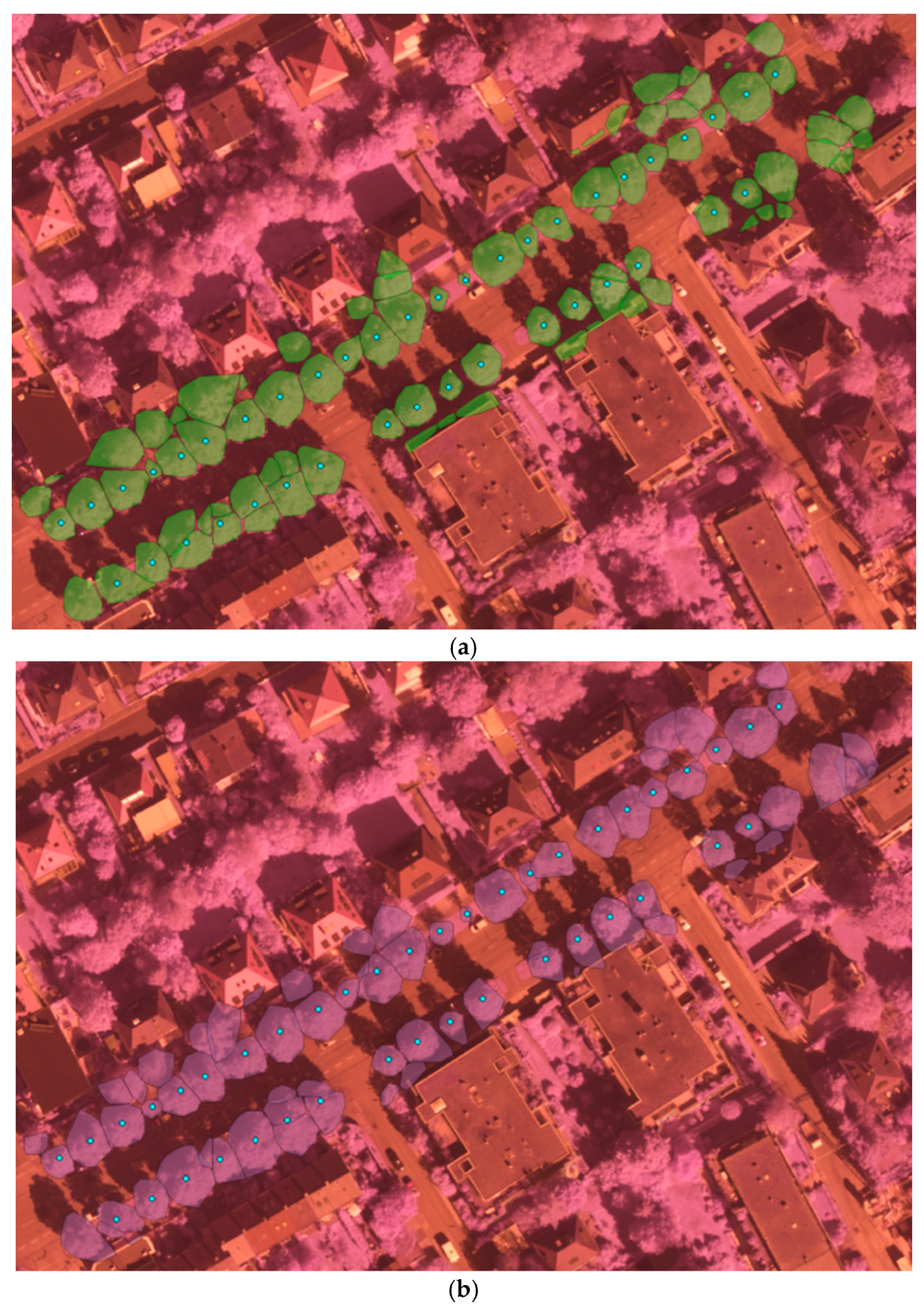
From the detection results in Figure 6, we can see that our method detected almost all the trees with ground truth. Through comparing the results of ALS and MLS, we can state that some trees’ contours derived from MLS were too large due to adjacent building points’ influence. As MLS collects data from the ground platform in a side-view perspective with a dense scanning of elevated surface, MLS data can’t cover upper part of high objects. It is greatly affected by the visibility along the scanning vehicle’s trajectory, in particular occlusions due to the presence of moving objects, buildings and trees etc. Thus, for the complicated scene in Figure 6, tree points with adjacent building points are prone to be segmented into larger trees and mixed small trees might be detected as one larger tree in the MLS data. Besides, some small structures of building tops and edges are also falsely detected as trees. On the other hand, the ALS collects data in a nadir (top-down) view perspective with aerial platform and less dense scanning at a high altitude, thus ALS data can achieve wider area coverage and represent the non-occluded top surface well. Thus, the tree crowns were extracted more accurately, which can be observed from Figure 6a. The point density is also an important factor in tree detection. It’s difficult and almost impossible to detect trees from sparse points. In the experiment two small ground truth trees(in Figure 6a, the two yellow arrows direct the two undetected small trees) were not correctly detected as depicted in Figure 6a in the relatively less dense ALS data, while they were both correctly detected in the MLS data. Overall, the detection accuracy from MLS data was worse than ALS data, though the MLS data was with much higher density. Higher density is not equivalent to better detection accuracy, the more complete and better data coverage of trees can be more important.

Comparing the tree attributes classification results from ALS and MLS data summarized in Table 11, it shows the ALS dataset obtained better accuracy for both the species and vitality using the MLR classifier. Thus, features extracted from the data collected in different view perspectives mainly caused the differences in attribute classification accuracy. In the experiment, features were extracted and selected with same approach from the detected tree points collected in different scanning perspectives: nadir (top-down ALS) view versus side view (MLS). As analysed and discussed above, view perspectives for LiDAR data collection have impact on the extraction accuracy of tree crowns, which further influences the correctness and reliability of the feature extraction for single trees. The selected features were arranged and listed in Table 2 according to the feature importance for classification. From Table 2, we can derive: (1) fewer features were selected from the ALS data, which means fewer features from nadir view collected data are essential to describe the tree attributes; (2) fewer features were selected for species classification, which means it needs more essential features to determine health status than classify tree species with LiDAR remote sensing data; (3) intensity feature S1_I and S2_I from ALS data were selected as the most important LiDAR features for determining tree species and vitality respectively in this experiment, while no intensity feature from MLS data was selected. The MLS intensity from side-view mode suffers from strongly varying incident angles and ranging distances, causing the intensity feature’s inconsistency; (4) compared to species classification, more LiDAR geometric features were selected for classifying tree vitality especially from the MLS data. The MLS scans the trees from a side-view perspective and can model their vertical structure in much more detail with dense point clouds, thus more internal geometric features from MLS can contribute to the tree vitality classification in the experiment; (5) as we used the infrared imagery which is very useful for vegetation classification, the image intensity related features for singles trees detected by LiDAR point clouds played an important role in tree attributes classification.

Better classification accuracy was achieved through fusing MLS and ALS classification probability outputs, which demonstrated that there exists complementary information useful for tree attributes classification. This is in compliance with the fact that MLS and ALS data were collected in different view perspectives, recording information describing the tree structure in different ways. Similarly, tree crown structure was accurately reconstructed through fusing the complementary perspective of ALS with the ultra-dense scanning of TLS in [15].

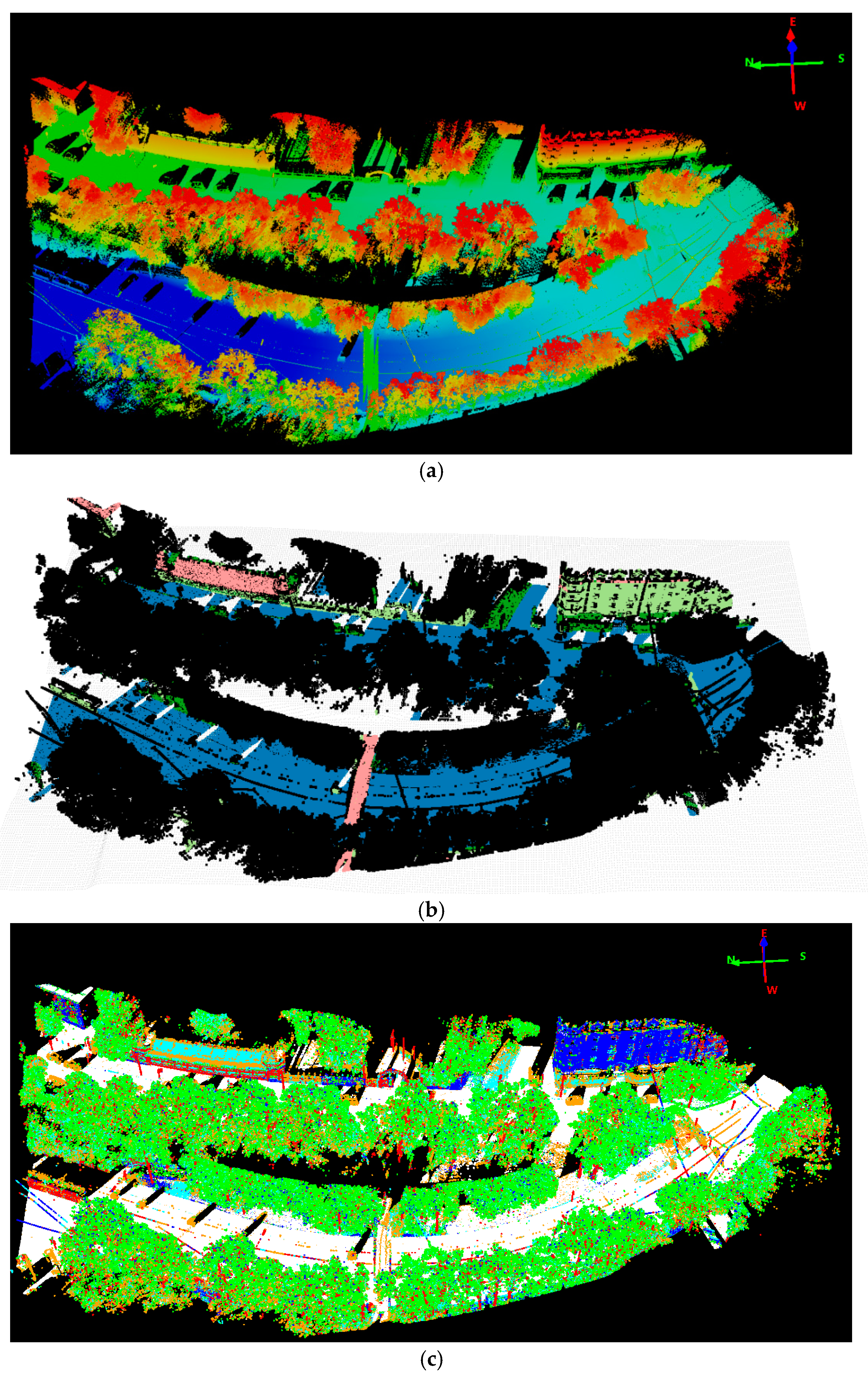
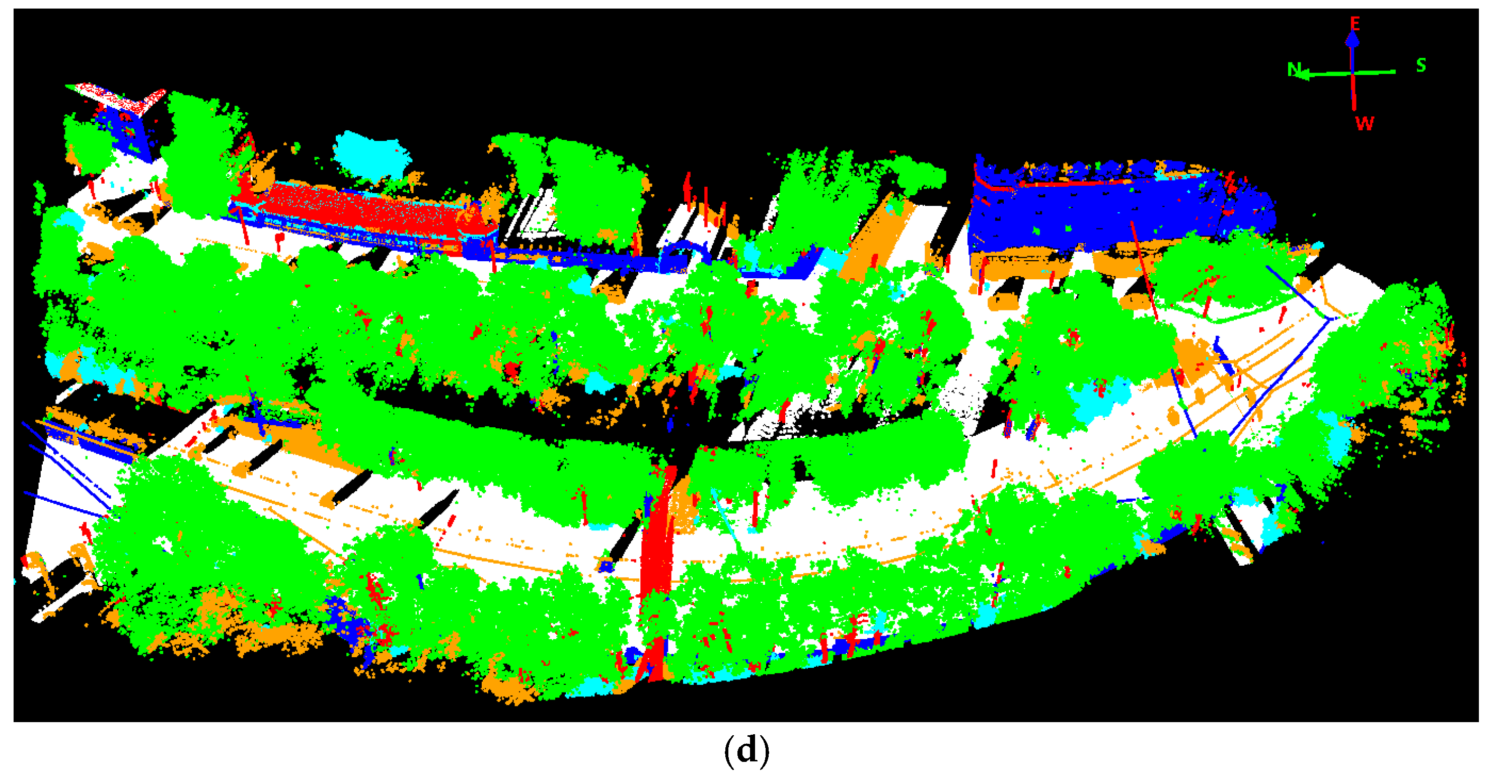
The different scanning perspectives also result in the difference of data collection cost and efficiency: ALS collects data more quickly and efficiently but less flexibly than the MLS as ALS is more likely to be constrained by weather conditions; it also costs more for ALS than MLS to enable the data collection in specific areas. However, more intensive computation arises for the MLS data. In our approach, a new method for the semantic labeling of ultra-high point density MLS data is developed based on combining a CRF for the context-based classification of 3D point clouds with shape priors, which makes the final point labeling results look smoother for the MLS data as depicted in Figure 4d. To cope with the ultra-high point density and maintain a graph structure of rational size for CRF solution, a plane-based region growing method combined with a rule-based classifier is applied to first generate semantic labels for man-made objects. Once these kind of points, that usually account for up to 60% proportion of the entire data set, are pre-labelled, the CRF classifier can be solved by optimizing the discriminative probability for nodes within a subgraph structure excluded from those nodes assigned with pre-fixed labels. Moreover, through the pre-labeling of planar structures, the scene can often be partitioned into disjoint regions whose labels no longer interact, and hence can be optimized independently.

Compared to traditional field work and laboratory measurement methods [35,36,37], tree vitality classification by remote sensing is a relatively new and challenging task, especially at the single tree level. Within our experiment, the infrared imagery features contributed more than point cloud features, which could be induced from Table 2. Almost all existing studies from remote sensing community mainly adopted spectral and image features for tree vitality or condition classification with aerial or space-born platform [38,39,40,41,42,43,44], and studies using LiDAR related features for tree vitality classification are seldom reported. Our experiments demonstrated that the infrared features are more powerful than both the MLS and ALS data for tree vitality determination. On the other hand, laser scanning can acquires tree structure more accurately which can be used to assess the tree health status [45]. From Table 2 it can also be deduced that the MLS geometric features contribute more than that of ALS to tree vitality classification, which is attributed to the capability of MLS to scan the tree vertical structure in much more details from side-view.

Although a re-balancing process was conducted to adjust great differences in training sample size per class, it should be noted that the imbalanced sample sizes in our experimental data still influenced the classification accuracy: the number of Robinia trees was much smaller than other species, and training samples for trees of growing health level 2 were too few compared to other tree growing health levels, which can be observed from Table 3, Table 4, Table 5 and Table 6. Tree species and vitality classes with similar sample sizes could even improve the classification results. Through analyzing Table 8 and Table 10 for confusion-matrix of tree vitality classification, it can be observed that there was a relatively higher confusion between 1+ and 1- category than that between 1+ and 1 or between 1 and 1−. The reason is that almost all the tree samples with growth health level 1 belong to Dutch linden, while tree samples with 1+ and 1- category are evenly distributed across all 4 species.

As ALS and MLS data were collected in two different platforms, fine registration is essential for their data level fusion. In our experiment, only accurate georeferencing process was conducted on the ALS and MLS data respectively, which achieved good geolocation accuracies. However, no mutual fine registration was applied to the ALS and MLS data which impeded a data-level fusion at the beginning. To combine the tree attribute classification results of ALS and MLS data, we selected the nearest trees extracted from MLS data as the corresponding trees to ALS data. This relatively simple process may encounter nonalignment problem which will cause fusion errors in the complicated environment. Single tree level attributes should be studied as the constraints to find corresponding trees between ALS and MLS data in the further work. It consists of many processing steps for single tree level mapping. Accurate semantic labeling of the LiDAR data is the basis of good tree detection results. Tree detection error can reduce classification accuracy: the adjacent trees with clumped crowns are easy to be detected as one tree which will cause wrong classification results. Besides, the accuracy of detected trees’ contour also influences the extraction of trees’ features, which has direct impact on the classification accuracy.

5. Conclusions and Future Work

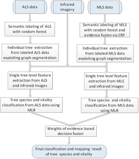
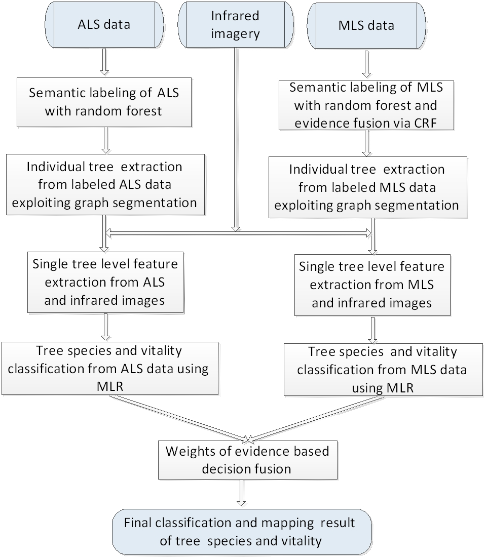
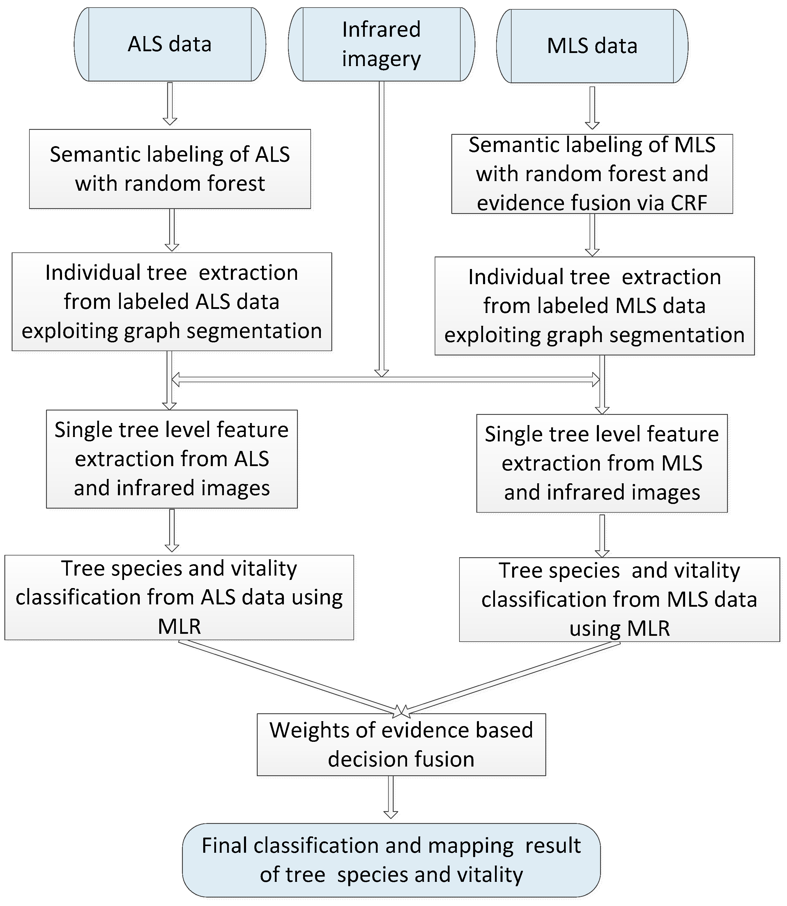
In this work, we studied and compared the urban tree mapping potential of ALS and MLS data in terms of performance in detecting trees and recognizing their species and vitality. A complete approach was presented, including semantic labeling for point cloud, single tree detection and feature extraction, classification of tree species and vitality, and decision fusion of ALS and MLS classification outputs to enhance final mapping results. To make better point-wise semantic labeling for the highly dense MLS data, an improved framework for combining the point-wise class labeling results of RF and local contexts was proposed, which reduces the highly intensive computation efficiently and makes it possible to accurately label ultra-dense point clouds through CRF smoothing.

Through comparing ALS based and MLS based methods, we can conclude: (1) LiDAR scanning perspective is a greatly influential factor for tree detection rate and classification accuracy of tree species and vitality. In our experiment, ALS based methods achieved better accuracy of both the tree detection and classification of the two tree attributes. ALS can cover the tree top surface more completely with nadir scanning perspective, which is very useful for tree detection and tree feature extraction; in contrast, MLS collects data in a side-view perspective and collected tree points are always affected by the adjacent man-made objects like buildings. Contours of tree crowns extracted from ALS are more accurate than that from MLS, which contribute to extraction of more accurate tree features; (2) Higher density is helpful for deriving better geometric features but not equivalent to yielding better mapping accuracy. MLS achieves much higher density data and can retrieve vertical structure information of trees in much more details. In our experiment, more geometric features from MLS were selected for determining tree health status than that from ALS. However, MLS still obtained worse accuracy than ALS for determining tree vitality; (3) Only use of ALS data can lead to satisfactory results for tree detection and characterization in urban road corridors, and even better accuracy can be achieved through fusing the complementary information of the ALS and MLS data. Applying the approach presented in this work to the ALS data only, we achieved tree detection accuracy of 83.6%, species classification accuracy of 72.19% and vitality classification accuracy of 68.89% under the complicated urban road environment. To make use of the complementary information of the ALS and MLS data, a weight of evidence based decision method was adopted to improve the tree attributes classification accuracy. In our experiment, the fusion methods achieved an overall accuracy of 77.89% for tree species classification and 73.53% for tree vitality classification, which was better than the method based on a single data source for both ALS and MLS.

Since there exists good complementarity between ALS and MLS in terms of different scanning perspectives and platforms, point density, ranging distance and data coverage, ALS and MLS data can be further combined to solve more challenging tasks such as fine tree structure modeling, accurate carbon stock estimation and so on in the future work. As these two data sources are collected from different platforms, the fine registration of ALS and MLS data needs further study to handle the redundancy for various applications.

References

1. Nowak, D.J.; Crane, D.E.; Stevens, J.C. Air pollution removal by urban trees and shrubs in the United States. Urban For. Urban Green. 2006, 4, 115–123. [Google Scholar] [CrossRef] [Green Version]
2. Xiao, Q.; Mcpherson, E.G. Rainfall interception by Santa Monica’s municipal urban forest. Urban Ecosyst. 2002, 6, 291–302. [Google Scholar] [CrossRef]
3. Mcpherson, E.G.; Simpson, J.R. Potential energy savings in buildings by an urban tree planting programme in California. Urban For. Urban Green. 2003, 2, 73–86. [Google Scholar] [CrossRef]
4. Amiri, N.; Yao, W.; Heurich, M.; Krzystek, P.; Skidmore, A.K. Estimation of regeneration coverage in a temperate forest by 3D segmentation using airborne laser scanning data. Int. J. Appl. Earth Obs. Geoinform. 2016, 52, 252–262. [Google Scholar] [CrossRef]
5. Kankare, V.; Liang, X.; Vastaranta, M.; Yu, X.; Holopainen, M.; Hyyppä, J. Diameter distribution estimation with laser scanning based multisource single tree inventory. ISPRS J. Photogramm. Remote Sens. 2015, 108, 161–171. [Google Scholar] [CrossRef]
6. Tanhuanpää, T.; Vastaranta, M.; Kankare, V.; Holopainen, M.; Hyyppä, J.; Hyyppä, H.; Raisio, J. Mapping of urban roadside trees—A case study in the tree register update process in Helsinki City. Urban For. Urban Green. 2014, 13, 562–570. [Google Scholar] [CrossRef]
7. Holopainen, M.; Kankare, V.; Vastaranta, M.; Liang, X.; Lin, Y.; Vaaja, M.; Kukko, A. Tree mapping using airborne, terrestrial and mobile laser scanning—A case study in a heterogeneous urban forest. Urban For. Urban Green. 2013, 12, 546–553. [Google Scholar] [CrossRef]
8. Dalponte, M.; Bruzzone, L.; Gianelle, D. Tree species classification in the Southern Alps based on the fusion of very high geometrical resolution multispectral/hyperspectral images and LiDAR data. Remote Sens. Environ. 2012, 123, 258–270. [Google Scholar] [CrossRef]
9. Deng, S.; Katoh, M.; Yu, X.; Hyyppä, J.; Gao, T. Comparison of tree species classifications at the individual tree level by combining ALS data and RGB images using different algorithms. Remote Sens. 2016, 8, 1034. [Google Scholar] [CrossRef]
10. Piiroinen, R.; Heiskanen, J.; Maeda, E.; Viinikka, A.; Pellikka, P. Classification of tree species in a diverse African agroforestry landscape using imaging spectroscopy and laser scanning. Remote Sens. 2017, 9, 875. [Google Scholar] [CrossRef]
11. Shen, X.; Cao, L. Tree-species classification in subtropical forests using airborne hyperspectral and LiDAR data. Remote Sens. 2017, 9, 1180. [Google Scholar] [CrossRef]
12. Moghaddam, M.; Dungan, J.L.; Acker, S. Forest variable estimation from fusion of SAR and multispectral optical data. IEEE Trans. Geosci. Remote Sens. 2002, 40, 2176–2187. [Google Scholar] [CrossRef]
13. Cremon, É.H.; de Fátima Rossetti, D.; Zani, H. Classification of vegetation over a residual megafan landform in the amazonian lowland based on optical and SAR imagery. Remote Sens. 2014, 6, 10931–10946. [Google Scholar] [CrossRef]
14. Kosaka, N.; Akiyama, T.; Tsai, B.; Kojima, T. Forest type classification using data fusion of multispectral and panchromatic high-resolution satellite imageries. In Proceedings of the IEEE International Geoscience and Remote Sensing Symposium, IGARSS ’05, Seoul, South Korea, 29 July 2005; pp. 2980–2983. [Google Scholar]
15. Paris, C.; Kelbe, D.; van Aardt, J.; Bruzzone, L. A novel automatic method for the fusion of ALS and TLS lidar data for robust assessment of tree crown structure. IEEE Trans. Geosci. Remote Sens. 2017, 55, 3679–3693. [Google Scholar] [CrossRef]
16. Lefèvre, S.; Tuia, D.; Wegner, J.D.; Produit, T.; Nassaar, A.S. Toward seamless multiview scene analysis from satellite to street level. Proc. IEEE 2017, 105, 1884–1899. [Google Scholar] [CrossRef]
17. Li, X.; Zhang, C.; Li, W.; Richard, R.; Meng, Q.; Zhang, W. Assessing street-level urban greenery using Google Street View and a modified green view index. Urban For. Urban Green. 2015, 14, 675–685. [Google Scholar] [CrossRef]
18. Berland, A.; Lange, D.A. Google Street View shows promise for virtual street tree surveys. Urban For. Urban Green. 2017, 21, 11–15. [Google Scholar] [CrossRef]
19. Wegner, J.D.; Branson, S.; Hall, D.; Schindler, K.; Perona, P. Cataloging public objects using Aerial and street-level images—Urban trees. In Proceedings of the 2016 IEEE Conference on Computer Vision and Pattern Recognition (CVPR), Las Vegas, NV, USA, 27–30 June 2016; pp. 6014–6023. [Google Scholar]
20. Yao, W.; Polewski, P.; Krzystek, P. Semantic labelling of ultra dense MLS point clouds in urban road corridors based on fusing CRF with shape priors. In Proceedings of the International Archives Photogrammetry, Remote Sensing and Spatial Information Sciences, Wuhan, China, 18–22 September 2017; Volume XLII-2/W7, pp. 971–976. [Google Scholar]
21. Guyon, I.; Elisseeff, A. An introduction to variable and feature selection. J. Mach. Learn. Res. 2003, 3, 1157–1182. [Google Scholar]
22. Weinmann, M.; Schmidt, A.; Mallet, C. Contextual classification of point cloud data by exploiting individual 3D neighborhoods. In Proceedings of the ISPRS Annals of Photogramm., Remote Sensing and Spatial Information Sciences, Munich, Germany, 25–27 March 2015; Volume II-3/W4, pp. 271–278. [Google Scholar]
23. Rabbani, T.; Van Den Heuvel, F.; Vosselmann, G. Segmentation of point clouds using smoothness constraint. Int. Arch. Photogramm. Remote Sens. Spat. Inf. Sci. 2006, 36, 248–253. [Google Scholar]
24. Boykov, Y.Y.; Jolly, M.P. Interactive graph cuts for optimal boundary & region segmentation of objects in N-D images. In Proceedings of the Eighth IEEE International Conference on Computer Vision. ICCV 2001, Vancouver, BC, Canada, 7–14 July 2001; Volume 1, pp. 105–112. [Google Scholar]
25. Yao, W.; Krzystek, P.; Heurich, M. Tree species classification and estimation of stem volume and DBH based on single tree extraction by exploiting airborne full-waveform LiDAR data. Remote Sens. Environ. 2012, 123, 368–380. [Google Scholar] [CrossRef]
26. Shi, J.; Malik, J. Normalized cuts and image segmentation. IEEE Trans. Pattern Analysis Mach. Intell. 2000, 22, 888–905. [Google Scholar] [Green Version]
27. Reitberger, J.; Krzystek, P.; Stilla, U. Analysis of full waveform LIDAR data for the classification of deciduous and coniferous trees. Int. J. Remote Sens. 2008, 29, 1407–1431. [Google Scholar] [CrossRef]
28. Amiri, N.; Polewski, P.; Yao, W.; Heurich, P.; Krzystek, A.S. Feature relevance assessment for single tree species classification using ALS point clouds and aerial imagery. In Proceedings of the Young Professionals Conference on Remote Sensing, Cologne, Germany, 20–21 October 2016. [Google Scholar]
29. Haralick, R.M.; Shanmugam, K. Textural features for image classification. IEEE Trans. Syst. Man Cybern. 1973, 6, 610–621. [Google Scholar] [CrossRef]
30. Fassnacht, F.E.; Latifi, H.; Stereńczak, K.; Modzelewska, A.; Lefsky, M.; Waser, L.T.; Ghosh, A. Review of studies on tree species classification from remotely sensed data. Remote Sens. Environ. 2016, 186, 64–87. [Google Scholar] [CrossRef]
31. Jianwei, W.; Yao, W.; Zhang, J.; Li, Y. 3D semantic labeling of ALS data based on domain adaption by transferring and fusing random forest models. In Proceedings of the ISPRS TC III Symposium 2018, Beijing, China, 7–10 May 2018. [Google Scholar]
32. Bishop, C.M. Pattern Recognition and Machine Learning (Information Science and Statistics); Springer-Verlag: New York, NY, USA, 2006. [Google Scholar]
33. Good, I.J. Weight of Evidence: A Brief Survey. Bayesian Stat. 1985, 1, 249–269. [Google Scholar]
34. Song, B.; Li, P. A novel decision fusion method based on weights of evidence model. Int. J. Image Data Fusion 2014, 5, 123–137. [Google Scholar] [CrossRef]
35. Allikmäe, E.; Laarmann, D.; Korjus, H. Vitality assessment of visually healthy trees in Estonia. Forest 2017, 8, 223. [Google Scholar] [CrossRef]
36. Reichmuth, A.; Henning, L.; Pinnel, N.; Bachmann, M.; Rogge, D. Early detection of vitality changes of multi-temporal Norway spruce laboratory needle measurements—The ring-barking experiment. Remote Sens. 2018, 10, 57. [Google Scholar] [CrossRef]
37. Callow, D.; May, P.; Johnstone, D.M. Tree vitality assessment in urban landscapes. Forests 2018, 9, 279. [Google Scholar] [CrossRef]
38. Entcheva Campbell, P.K.; Rock, B.N.; Martin, M.E.; Neefus, C.D.; Irons, J.R.; Middleton, E.M.; Albrechtova, J. Detection of initial damage in Norway spruce canopies using hyperspectral airborne data. Int. J. Remote Sens. 2004, 25, 5557–5584. [Google Scholar] [CrossRef]
39. Xiao, Q.; McPherson, E.G. Tree health mapping with multispectral remote sensing data at UC Davis, California. Urban Ecosyst. 2005, 8, 347–359. [Google Scholar] [CrossRef]
40. Lambert, J.; Denux, J.-P.; Verbesselt, J.; Balent, G.; Cheret, V. Detecting clear-cuts and decreases in forest vitality using MODIS NDVI time series. Remote Sens. 2015, 7, 3588–3612. [Google Scholar] [CrossRef]
41. Näsi, R.; Honkavaara, E.; Blomqvist, M.; Lyytikäinen-Saarenmaa, P.; Hakala, T.; Viljanen, N.; Kantola, T.; Holopainen, M. Remote sensing of bark beetle damage in urban forests at individual tree level using a novel hyperspectral camera from uav and aircraft. Urban For. Urban Green. 2018, 30, 72–83. [Google Scholar] [CrossRef]
42. Fassnacht, F.E.; Latifi, H.; Ghosh, A.; Joshi, P.K.; Koch, B. Assessing the potential of hyperspectral imagery to map bark beetle-induced tree mortality. Remote Sens. Environ. 2014, 140, 533–548. [Google Scholar] [CrossRef]
43. Näsi, R.; Honkavaara, E.; Lyytikäinen-Saarenmaa, P.; Blomqvist, M.; Litkey, P.; Hakala, T.; Viljanen, N.; Kantola, T.; Tanhuanpää, T.; Holopainen, M. Using UAV-based photogrammetry and hyperspectral imaging for mapping bark beetle damage at tree-level. Remote Sens. 2015, 7, 15467–15493. [Google Scholar] [CrossRef]
44. Zagajewski, B.; Tømmervik, H.; Bjerke, J.W.; Raczko, E.; Bochenek, Z.; Kłos, A.; Jarocińska, A.; Lavender, S.; Ziółkowski, D. Intraspecific Differences in Spectral Reflectance Curves as Indicators of Reduced Vitality in High-Arctic Plants. Remote Sens. 2017, 9, 1289. [Google Scholar] [CrossRef]
45. Zarnoch, S.J.; Bechtold, W.A.; Stolte, K.W. Using crown condition variables as indicators of forest health. Can. J. For. Res. 2004, 34, 1057–1070. [Google Scholar] [CrossRef]
Figure 1. Overall workflow.
Remotesensing 10 01403 g001
Figure 2. Workflow for semantic labeling of point clouds.
Remotesensing 10 01403 g002
Figure 3. Workflow for single tree attributes classification based on weight-of-evidence (WofE) fusion.
Remotesensing 10 01403 g003
Figure 4. MLS dataset rendered by height (a) and its labeling by (b) pre-classification using plane fitting and heuristic rules plane fitting and heuristic rules (light blue = ground, light green = facade, pink = roof, dark green = low vegetation and car, black = tree); (c) random forest (RF) and (d) conditional random field (CRF) classification (white = ground, blue = facade, orange = car and low vegetation, green = tree, red = roof and pole).
Remotesensing 10 01403 g004aRemotesensing 10 01403 g004b
Figure 5. Single tree detection results of (a) Seybothstr ALS data and (b) Seybothstr MLS data.
Remotesensing 10 01403 g005
Figure 6. Single tree detection results of (a) Liebig ALS data; (b) Liebig MLS data.
Remotesensing 10 01403 g006