Satellite-Based Water Consumption Dynamics Monitoring in an Extremely Arid Area

Abstract

Evapotranspiration (ET) involves actual water consumption directly from the land surface; however, regional ET maps are usually neglected during water management and allocation. In this study, an integrated satellite-based ET monitoring approach with two spatial resolutions is proposed over an extremely arid basin in China that has experienced crop area expansion and has been the focus of a water-saving project since 2012. The proposed ETWatch approach combined with an empirical downscaling strategy based on vegetation condition was employed to produce monthly ET maps. This method achieves satisfactory accuracy and is validated by its reasonable spatial and temporal pattern results. Yearly results exhibit an increasing ET trend before 2012, which subsequently gradually decrease. This trend fits well with the dynamics of the basin-wide vegetation condition, indicating that there is a stronger correlation between water consumption and vegetation than between other environmental indicators. The average ET over three main crop types in the region (grape, cotton, and melon) decreased by approximately 5% due to optimizations of the irrigation timeline during the project, while 13% of the water savings can be attributed to the fallowing of crop areas. Based on the irrigation distribution in 2012, a comparison between drip and border irrigation that achieves water savings of 3.6% from grape and 5.8% from cotton is conducted. However, an afforestation project that involved planting young trees led to an approximate 25% increase in water consumption. Overall, since 2012, the water-saving project has achieved satisfactory performance regarding excessive groundwater withdrawal, showing a reduction trend of 3 million m³/year and an increase in Lake Aiding water levels since 2011. The results reveal the potential of the ET monitoring strategy as a basis for basin-scale water management.

1. Introduction

There are longstanding concerns that freshwater resources are insufficient to satisfy the increasing demand from various segments of human society. However, water allocation is slanted towards industry and domestic use primarily due to their economic benefits. Therefore, a dwindling agricultural water supply due to inadequate allocation is becoming a barrier to agriculture and husbandry in some parts of the world, even areas where farming lifestyles have been dominant for hundreds of years. Agricultural regions with arid climates such as the Nile basin in Egypt and Syria suffer from additional water stress due to an imbalance between ET and precipitation, usually leading to over-exploitation of aquifers and even water-related conflicts [1,2].

Globally, the spatial inhomogeneity of water resources is primarily affected by climate, which is difficult to change with human action. However, local and regional water management and re-allocation could be conducted to match the local topography and land surface patterns to better utilize water storage and runoff patterns [3]. Studies to optimize water allocation have been proposed worldwide and are available to policy makers [4,5,6,7,8]. In addition to guiding water into appropriate areas, advanced irrigation technology (e.g., sprinkler and drip) can be applied to improve water use efficiency (WUE) by reducing non-beneficial soil consumption [9,10]. However, inadequate allocation and irrigation programmes provide no water-saving guarantees because they typically fail to consider the hydrological cycle as a whole system [11]. The relationship between water consumption dynamics in water-saving measures should also be considered. In reality, both systematic designation and stepwise policy optimization through monitoring are required.

Water conservation projects have been proposed to save water from several aspects, especially in the arid north-western areas of China. Except for dams built to store floodwater for the dry season, investments in China have mainly targeted improved water delivery infrastructure and irrigation technologies. However, these measures may not always achieve a reduction of real water consumption from crops [12]. Optimized infrastructure can greatly reduce percolation but provide no guarantee of real water saving. This approach simply allocates reduced water resources to specific uses. In fact, overall water consumption in a basin may even increase ET and exacerbate the water scarcity. It is easy to imagine a scenario in which growing high-value crops, such as fruit, becomes easier with sufficient water supply provided by the improved drainage and irrigation system, resulting in increased total water consumption due to the expansion of fruit cultivation. In some regions, a reduced water supply might be more susceptible to contamination by saline aquifer or runoff into the sea [11]. Due to the outmoded management strategies, in some parts of China, surface and groundwater over-exploitation resulting from irrigated agriculture has led to ecosystem deterioration [13]. Thus, conservation projects require both adoption and constant optimization with assistance from timely monitoring results to achieve true water savings.

Remote sensing (RS) images can provide spatially distributed, time-series data of the earth’s surface at diverse resolutions and have been proven to be a reliable source for monitoring water consumption [14,15,16]. Researchers worldwide have designed satellite-based ET models with satisfactory reliability [10,17,18]. Over the past decade, management and allocation projects have capitalized on satellite-based ET monitoring to relieve water stress [19,20,21]. Anderson lists several applications that employ moderate-resolution ET maps (30-m) to reflect the ecosystem response to water management [22]. In addition, an Operational Simplified Surface Energy Balance (SSEBop) model has been used to monitor water consumption in two American regions, including the Palo Verde Irrigation District, which has an arid climate [23,24]. The results show that there is a high correlation between total water consumption and human activity, especially with respect to irrigation in arid regions. ET from local plants consumes approximately 70% of total terrestrial rainfall [11]. Therefore, water consumption by vegetation should be effectively controlled and managed. However, due to differences in surface conditions, no universally applicable monitoring strategy exists. For example, large homogeneous farmland areas (over 100 ha) are rare in northwest China, which usually causes RS pixels to be mixed. Therefore, the 4-km pixels from reference ET data are not fine grained enough to reveal ET spikes after local irrigation [24]. Moreover, developing a unified spatial resolution of an ET map that is suitable for analysis from different aspects is impractical. Data with low spatial resolution are available at higher frequencies and over longer time series, but responses from ecosystems and human society to the water-saving policy are necessary to maintain a sustainable cycle, which could be monitored by more detailed analysis. Therefore, an integrated ET monitoring strategy should be designed and conducted considering different monitoring tasks and their corresponding resolution requirements.

In this study, an ET monitoring approach that uses two spatial resolutions was designed for the Turpan Oasis, which has an extremely arid climate. Since 2006, the region has experienced farmland expansion due to policy and migration from other provinces. In late 2011, the local government began investing in a water protection project, and drastic variations in agricultural and ecological policies make this area a valuable case study for water management monitoring. The main objectives of this study were: (a) to evaluate the monitoring strategy’s performance in an extremely arid region using data from 2006 to 2016; (b) to analyse the spatiotemporal dynamics by employing validated ET results; (c) to summarize the agriculture and ecological responses to the water-saving policy; and (d) to assess the successes and challenges in current ET monitoring strategy. Section 2 introduces the methods and data involved in this study. Section 3 presents ET simulation results and a detailed analysis based on ET monitoring. Section 4 provides a discussion of the entire monitoring study. Conclusions and a summary of the study are presented in Section 5.

2. Materials and Methods

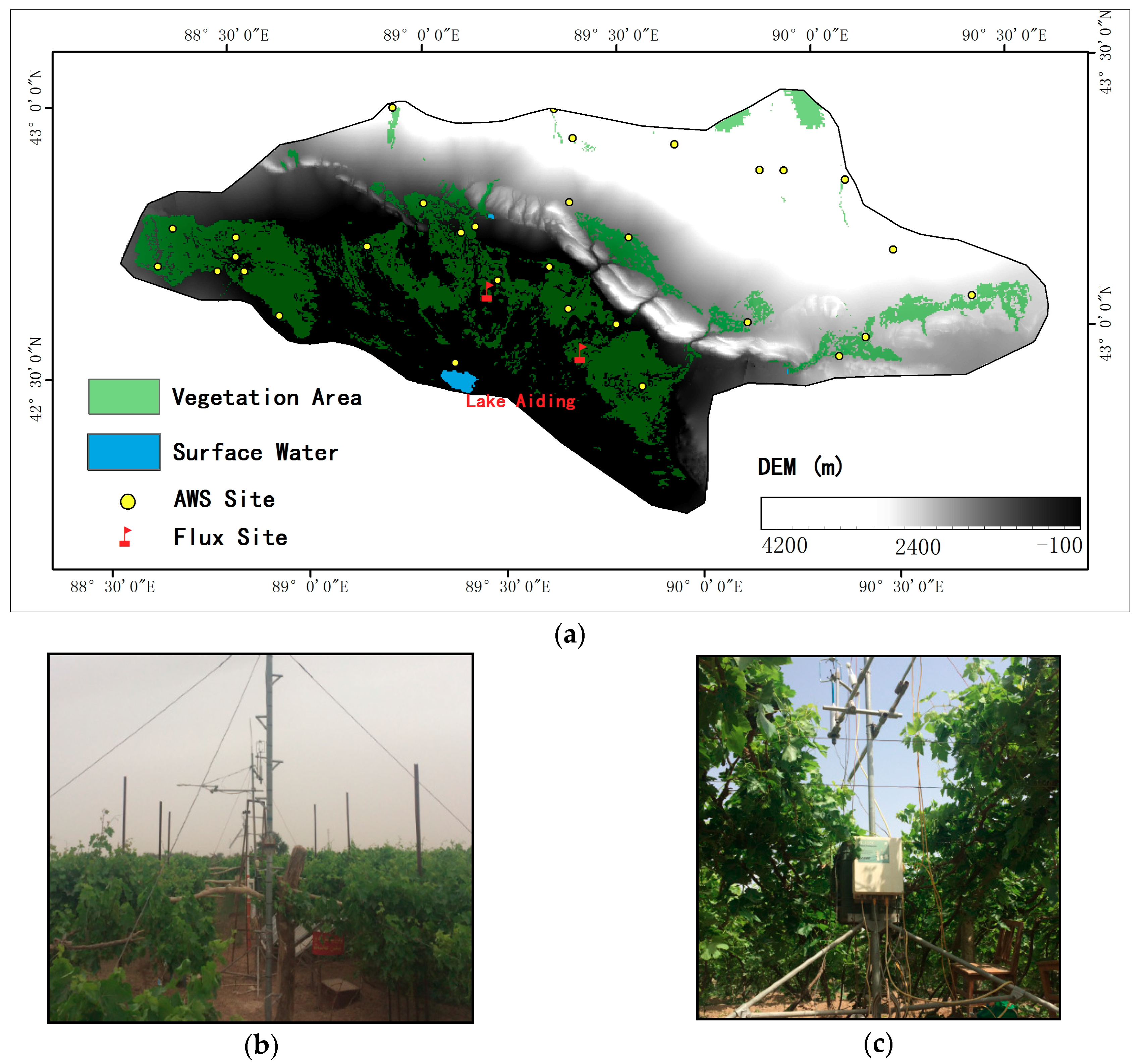
2.1. Research Area

Turpan Prefecture is located in the eastern part of the Xinjiang Uygur Autonomous Region, which is the most arid province in China. The prefecture’s total area is approximately 70,000 km² and includes the Turpan basin and a large area of Gobi land. The basin is surrounded by mountain ranges with snow-covered peaks rising nearly 5000 m above sea level in the north. The southern part of the region contains the second lowest point on earth, 155 m below sea level, which has a neighbouring salt swamp called Lake Aiding. The basin has been recorded as the hottest and most arid area in China, with average air temperatures above 40 °C in summer and less than 20 mm of annual precipitation. The hot, windy and dry climate causes the annual potential evaporation to exceed 2000 mm. The location of the Turpan basin with a digital elevation model (DEM) is shown in Figure 1a.

The Turpan basin contains a successful irrigated oasis with a long cultivation history. Available surface water in the oasis originates in the mountainous areas in the north and west and is supplied by snowmelt and rainfall. A complex canal system built by local residents guides water into every field. Irrigation is also conducted using groundwater acquired through the Karez water supply system, which is an ancient and unique water delivery system devised to avoid non-useful evaporation during water flow by employing underground drainage, and electrical pumps [25].

In total, approximately 20% of the water for irrigation comes from groundwater and the other 80% from the mountains. The dominant crop grown in the oasis is grape. Three main crop types, grape, cotton and melon, occupy approximately 75% of the total arable land area.

Turpan Oasis experienced a sharp expansion of irrigated land due to modern well-drilling technology. Cropland nearly doubled in 30 years, from 60 kilo-hectares (kha) in 1970 to approximately 100 kha in 2012. Basin-wide water consumption now exceeds the renewable supply, resulting in severe groundwater over-exploitation. On average, groundwater tables are declining by 1.5–2 m per year and have fallen by up to 180 m in some areas. Of the 1237 Karez systems that existed in 1957, fewer than 300 have running water today. The disappearance of the Karez systems and the decreasing groundwater have contributed to the degradation of the oasis ecosystems; Lake Aiding is nearly dry most of the year. Faced with this situation, the government has supported a pilot integrated water management project based on consumption that adopts satellite-based ET monitoring and has introduced basin-wide planning and water allocation schemes for the different sectors.

Supported by this project, an eddy covariance (EC) recorder equipped with an automatic weather system (AWS) was originally located in a basin over a grape field (89.58°E, 42.76°N). To improve management, the tower and its recorders were moved to another grape field (89.31°E, 42.84°N) in early 2016. The position and images of the two sites are shown in Figure 1. ET simulation involves records from 29 AWS stations administered by the local weather bureau; the positions of these AWS stations are also displayed in Figure 1a.

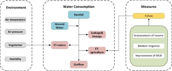
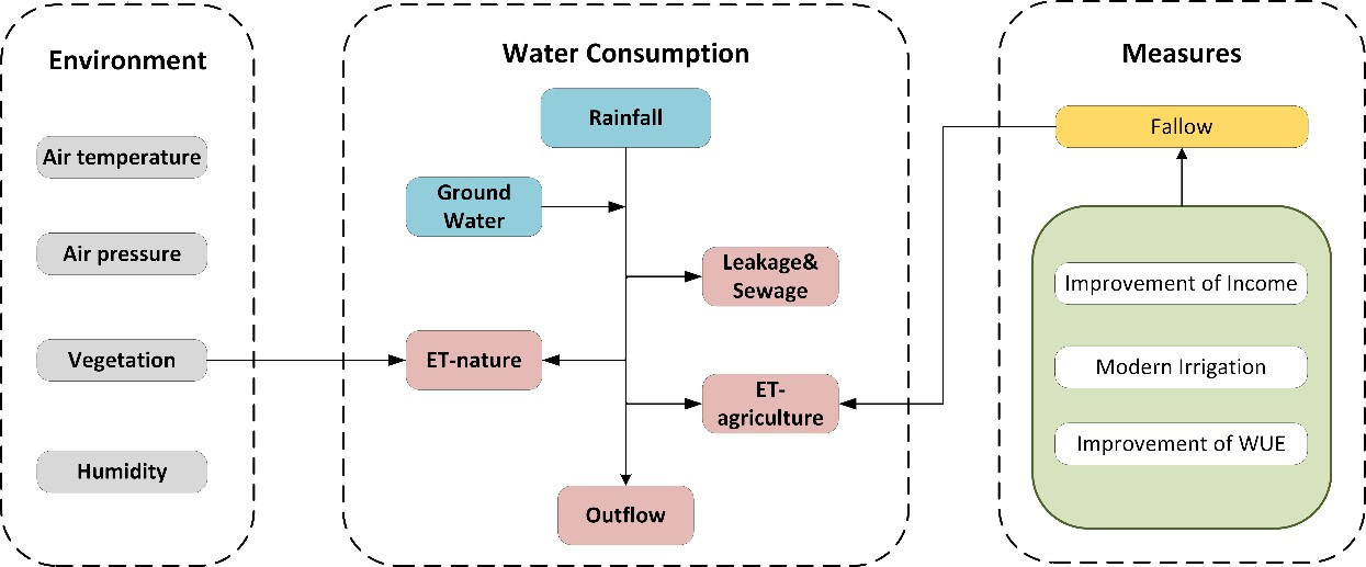
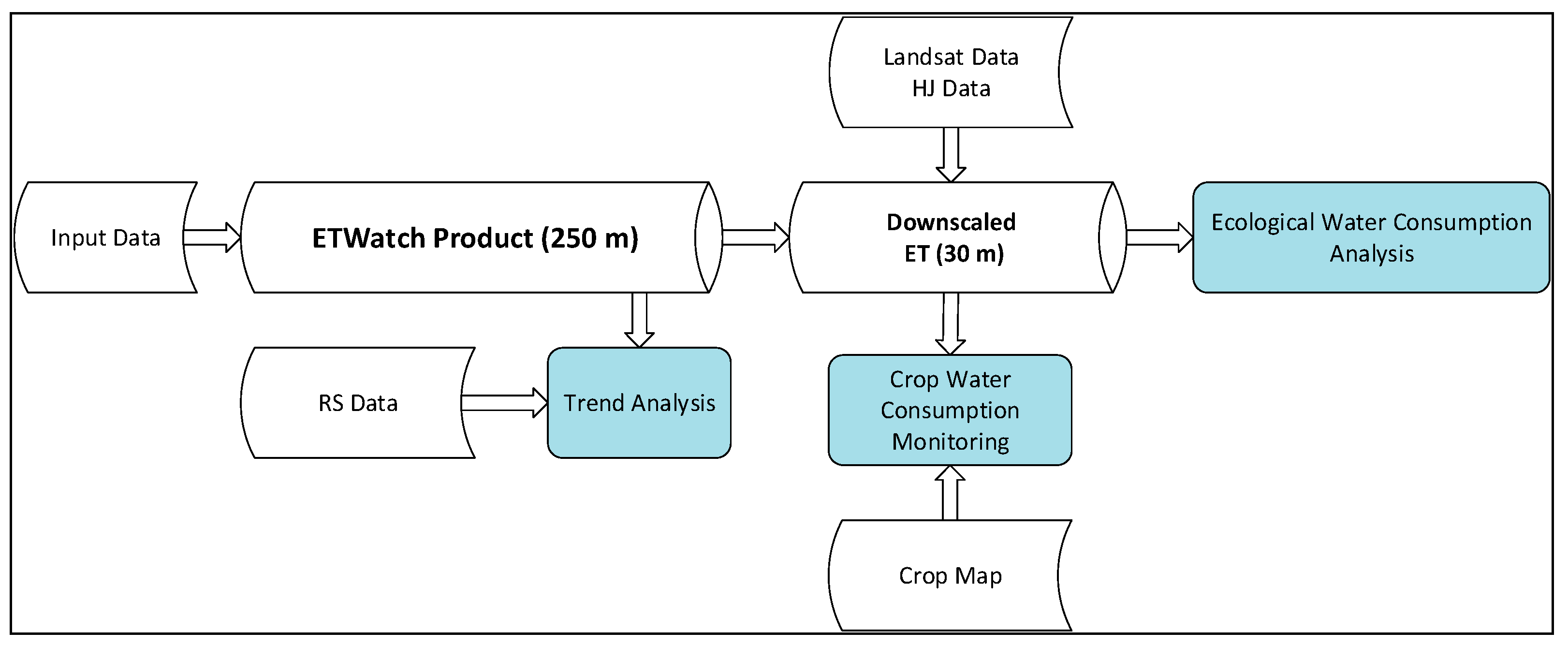
2.2. Monitoring Framework

Monitoring conducted in this study was designed to use ET maps with multiple spatial resolutions. Two levels of spatial resolution and temporal range were proposed, including corresponding ancillary data for different analysis purposes. Basin-wide spatial and temporal trend analysis was conducted with validated 250-m ETWatch products from 2006 to 2016, based on which the water consumption dynamics of the entire basin could be calculated. During this step, daily MODIS products were involved with smoothed meteorological observations as model inputs. This interpolation step was required because influences from topography should be taken into consideration for a regional meteorological analysis, especially in the current irregular hilly basin. Downscaled 30-m distributed ET from 2012 to 2016 was then employed to conduct a further analysis over farmland through a yearly crop map and monthly normalized difference vegetation index (NDVI) maps from Landsat images. This disaggregation step was required because the 250-m pixel resolution was insufficiently fine to achieve homogeneous field patches, which need to be provided by Landsat scale images. Figure 2 shows the overall workflow of the monitoring process.

An ET map at the 250-m level was first calculated using the ETWatch method, which has been validated in several regions under different climate types [15,26]. “Clear day ET” was simulated using the “Residue Approach”, which is based on the energy balance model. Instantaneous latent heat flux ($\lambda E$) was computed as the residue of the energy balance equation using data from satellite overpasses on cloud-free days.

$$R_n=\lambda E+H+G_0$$

(1)

where $R_n$ (W/m²) is the net radiation, $G_0$ (W/m²) is the soil heat flux, H (W/m²) is the sensible heat flux, and λE (W/m²) is the latent heat flux.

The $\lambda E$ from the instant of imaging was then extended to a full-day scale under the assumption that the evapotranspiration fraction (ef) is constant during every clear day [27]. An inverse of the Penman–Monteith (P-M) equation was employed to calculate surface resistance ($R_{sur}$). Daily net radiation was simulated by the Ångström–Prescott model [28,29,30,31], in which sunshine duration was estimated by Liu’s empirical strategy using the FengYun geostationary meteorological satellite (FY-2D) hourly cloud classification data [32]. Information on the planetary boundary layer (PBL) was extracted using Feng’s approach [33]. The time series of $R_{sur}$ was then reconstructed using the gap-filling algorithm to simulate water losses on cloudy days, taking the minimum air temperature ($T_{min}$), vapour pressure deficit (VPD), smoothed leaf area index (LAI), soil moisture content (SM) and net radiation ($R_n$) into account [15]. Finally, the daily ET for the whole year was calculated using the PM equation with routine meteorological observations as follows [34]:

$$\lambda E=\frac{sA+\rho C_p(e_{sat}-e_a)/R_a}{s+\gamma (1+R_{sur}/R_a)},$$

(2)

where λE (W/m²) is the latent heat flux, s is the slope of the curve relating saturated water vapour pressure to temperature, A (W/m²) is the available energy calculated using net radiation and soil heat flux, Rn is the net radiation flux, ρ (kg·m⁻³) is the air density, $C_p$ (J·kg⁻¹K⁻¹) is the specific heat of air, $(e_{sat}-e_a)$ is the vapour pressure deficit (VPD), γ (Pa·K⁻¹) is the psychrometric constant, $R_a$ is the aerodynamic resistance, and $R_{sur}$ is the surface resistance.

The resulting coarse ET map was then disaggregated to a 30-m scale using the empirical downscaling method recommended by Tan [35]. The downscaling step was conducted under the assumption that the 250-m pixels accurately represent the water consumption from the corresponding land surface. Then, we could calculate

$${\mathrm{ET}}_{30}={\mathrm{ET}}_{250}\times \frac{p_{30}}{p_{250}},$$

(3)

where ${\mathrm{ET}}_{30}$ is the downscaled ET result at a resolution of 30 m; ${\mathrm{ET}}_{250}$ is the actual ET (ETa) calculated from the 250-m MODIS data (ETWatch in this research); and $p_{30}$ and $p_{250}$ are the driving factors calculated from the 30-m resolution images and historical reports of water consumption, respectively.

Downscaling factor $p$ consists of the NDVI because water consumption in arid areas is dominated by vegetation. The historical ratio of NDVI/ETa was used to decrease the potential deviation because of heterogeneity of the land surface [35].

Only one NDVI image is usually available from Landsat during this step in Turpan due to cloud contamination. Consequently, the 30-m resolution ET maps were provided only at monthly intervals. The downscaling strategy described above allocates total ET in the coarse pixels (e.g., one MODIS pixel) into every single fine pixel (30-m pixel) rather than calculating ET independently. Water consumption amount in every coarse pixel remains invariable after disaggregation. However, regional water consumption between different resolutions increased slightly (approximately 10 mm per year) over every crop type during this step due to the concentration of ET from bare land in the mixed coarse pixels.

Next, an analysis combined with corresponding information was proposed to diagnose the water consumption variations, which are influenced by many aspects. The 250-m resolution ET map was mainly utilized in conjunction with regional meteorological parameters, such as air temperature and humidity, and the NDVI map was used to analyse temporal and spatial trends and their driving factors at the basin scale. In contrast, at the 30-m scale, yearly crop maps can be employed to monitor the water-saving performances of different crop types. Fallow farmland and optimized crop selection can also be monitored at this level. A detailed field survey of a sub-basin of the entire study region was completed in 2012 that included attributes such as irrigation types. Based on this survey, we proposed an analysis to investigate the performances of different irrigation strategies. Obtaining these results is important before encouraging the adoption of basin-scale drip irrigation.

2.3. Satellite Data

Three MODIS tiles (h23v04, h24v04 and h25v04) were needed to cover the entire Turpan region. The daily instantaneous surface pattern was simulated by MYD02, MYD09GA and MYD11A1 products. Surface reflectance from AQUA (MYD02 and MYD09GA) was used to retrieve surface parameters, such as NDVI and albedo, at 250-m and 500-m spatial resolutions. Land surface temperatures with abnormal pixels are recorded in MYD11A1, which can be used as a mask at the 1-km scale. However, artificial image selection was still needed to eliminate cloud contamination over the basin (or, at least, over the oasis). Images at approximately 100 days were chosen for every study year after this step.

For downscaling purposes, at least one 30-m resolution image was required every month during the growing season. Two tiles were needed to cover the whole basin (paths 141 and 142 and row 030). Tiles from the HuanJing (HJ) satellite of China (path 35, rows 60 and 64) were employed when no qualified image could be obtained from Landsat for a given month. Images from the two satellites share similar wavelength and spatial resolution (30 m), but shorter re-visiting intervals are used with the HJ satellite. However, a registration/matching step was still required to guarantee that the same pixel from two different sensors represents the same surface area. After this rectification process, we achieved less than one pixel of root mean square error (RMSE). Similar performances after downscaling have been observed from these two data sources based on Tan’s research [35].

2.4. Other Data

2.4.1. Land Cover and Crop Maps

China Cover, a nationwide land cover product, was employed to summarize and analyse ET over diverse surfaces at a 30-m resolution. The China Cover dataset is generated using an object-based method and updated every five years [36]. The overall accuracy of this dataset at the second level of classes is >86% [37]. This study included land cover maps from 2005, 2010 and 2015.

Farmland was optimized over the whole basin during the monitoring period; this includes retiring fields with relatively low WUE and converting cotton fields into fruit crops such as grape and melon. Other than grape, most of the crops in the oasis are annual. Thus, crop areas vary substantially from year to year, and this variation can be monitored with a RS-based crop map. Basin-wide crop monitoring was conducted for each year from 2012 to 2016 at a 30-m resolution using an object-based method that considers the phenological differences between the crops in this region.

2.4.2. Ancillary Datasets

Daily meteorological observations from 29 stations from Chinese Meteorological Administration and local bureau were spatially interpolated to form the input data for ETWatch, and the basin-wide analysis using this method takes elevation and topography into consideration. Parameters involved include air temperature, relative humidity, air pressure and wind speed after artificial checking of data quality. Basin-wide statistics used in the analysis, such as the use of chemical fertilizers and income from agriculture, were taken from the National Bureau of Statistics of the People’s Republic of China. Groundwater and inflow water were monitored by the local Bureau of Water Conservancy of Turpan City. The area of open water surface was provided by a global water surface product available on the Internet [38].

2.5. Trend Analysis

ET was monitored at MODIS scale with a relatively long time series (2006–2016) that covers the intensive variation period of irrigated agriculture in the Turpan basin. The time-series water consumption trend was analysed using a Mann–Kendal (M-K) trend test [39] at the basin scale. The non-parametric rank-based strategy has been widely used to analyse time-series trends in hydrological data by other researchers [40,41,42].

3. Results and Analysis

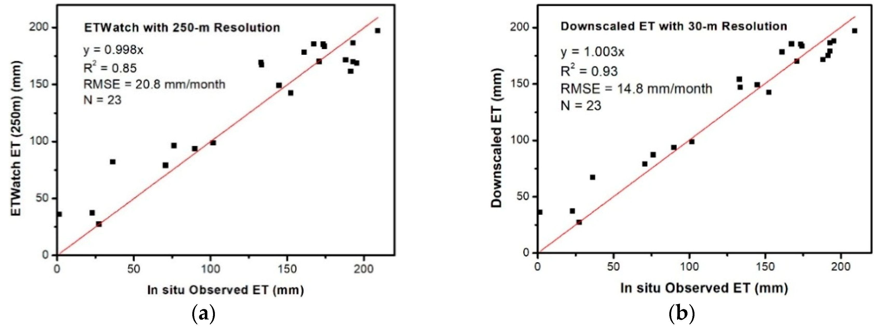
3.1. Evaluation of ET Estimates

ET monitoring at the 250-m resolution was acquired for 11 years, from 2006 to 2016. Spatially distributed ET maps covering the same time interval for 2006, 2011 and 2016 are presented in Figure 3a–c. There is an obvious difference in ET between vegetation and bare land. A high ET value comes from crop fields in most of the oasis and the wet areas around Lake Aiding in the south. Annual water consumption from bare soil and desert is typically less than 20 mm due to sparse precipitation, which is insufficient for growing plants. Fields in Toksun (in the western part of the oasis—separated from other regions by Gobi land) consume less water than those in other regions. This phenomenon is caused by strong winds in this region (daily average of approximately 2.5 m/s in this region, compared with 1.5 m/s over the entire oasis), which limits the growing of grape. Transpiration from annual herbaceous crops such as melon is not as high as that from grape.

An obvious time-series trend was observed in the middle and eastern portion due to increasing numbers of vineyards compared to other crop types, especially cotton. In total, water consumption increased before 2011 and reached a peak. Since then, retiring and fallowing farmland (due to the water-saving project) has led to a decreasing trend. Fallow fields typically occur in small patches (smaller than one pixel) in Turpan rather than across entire large farms. Although the oasis area seemingly remains invariable, the average ET over the vegetation pixels changes. Across the entire region, the most obvious decreasing ET trend occurred in Toksun due to the policy in this region to encourage the cultivation of crops that require less water, such as fast-growing melon and date trees.

The 30-m ET maps after disaggregation for the three years 2012, 2014 and 2016 are displayed in Figure 3d–f. The downscaled ET map supplements the spatial trend of the 250-m map by providing more details such as highways and access roads between fields. Thus, further analysis is mainly conducted on the 30-m ET maps in the following sections.

Because the hot, dusty and windy climate in the Turpan basin is harmful to the EC recorder, records from certain months had to be eliminated due to equipment maintenance. Finally, records from 23 months were available to validate the ETWatch dataset. Figure 4 presents the results of a comparison between the simulated ET at 250-m and 30-m resolutions and the in situ observations. The results indicate that the accuracy of modelled ET by ETWatch and downscaled dataset are satisfactory. The R² values range from 0.85 using the 250-m maps to 0.93 using the 30-m maps, and the RMSE values range from 20.8 mm/month to 14.8 mm/month. The results from the 30-m maps show obvious improvements due to the disaggregation of coarse pixels. A small patch of bare land exists northeast of the EC tower that could not be recognized on the 250-m map. The high estimated ET from this patch will be distributed across vegetation pixels during downscaling. A small increasing trend of fixed slope is thus observed in the 30-m validation (with a slope of 1.003 as opposed to 0.998). The water consumption from the mixed 250-m pixels is disaggregated into each 30-m grid, which improves the accuracy.

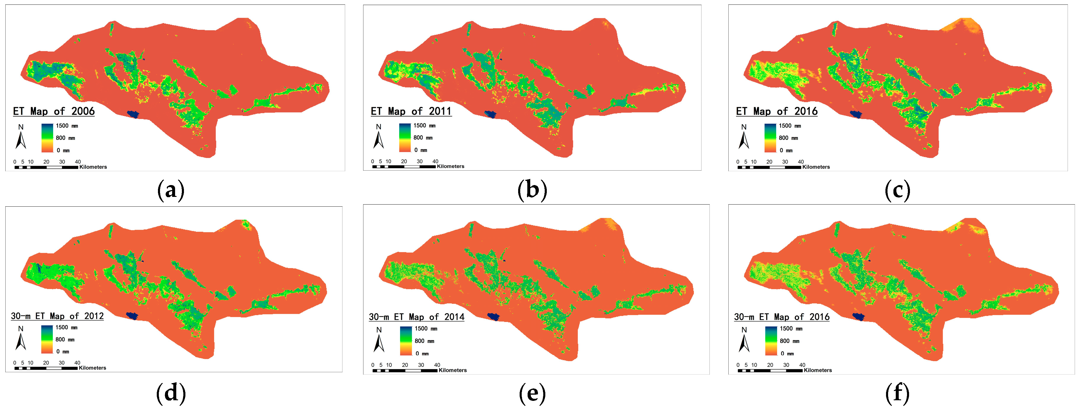
3.2. Water Consumption Dynamics

Characterization of water consumption dynamics is useful for basin-scale water management. Variations in ET response could provide effective optimization information for decision makers. In the current research, the annual average ET (ETa) is summarized to help detect temporal trends over the whole basin. Yearly variations of relative environmental indicators such as NDVI, air temperature (Ta) and relative humidity (humd_rel) are also illustrated in Figure 5. In this research, time-series NDVI maps after Savitzky–Golay filtering covering the entire growing season (April to October) were employed to calculate yearly average area with vegetation cover [43]. Annual precipitation was not investigated because, unlike in other regions, rainfall scarcely affects water consumption in this region [24,42]. According to the results of the M-K test, the ETa from Turpan displays a non-significant increasing trend starting in 2006 with a slope of 0.70. Average water consumption reached a peak of 128.6 mm in 2012 and decreased gradually thereafter but remained higher than in 2006. This trend is confirmed by the ET map shown in Figure 3. The non-significant increasing is caused by the re-decreasing phenomenon since 2012. No other indictor shows a similar increasing trend except NDVI. Figure 5b shows that the increase in ET is positively related to NDVI (R² = 0.61). Crops in extreme areas can be cultivated only with irrigation. Therefore, it is reasonable to conclude that better plant conditions, which are reflected by higher NDVI, lead to increased water consumption. T_a and humd_rel display neither significant temporal trends nor correlations with water consumption (R² values of 0.23 and 0.37, respectively). In addition, an increase in NDVI leads to a slight decrease in the average air temperature, which is typically positively correlated with ETa. The opposite trend in Turpan indicates that the ETa is more sensitive to variations in vegetation than to variations in air temperature in arid regions.

3.3. Agricultural Water Consumption

Total ET is mainly affected by vegetation in the Turpan basin. The analysis in the current and following sections addresses water consumption over cropland and ecological regions, respectively. A comparison of inflow water, actual water consumption across the entire basin and cropland is displayed in Figure 6a. From the monitoring results, we can conclude that water inflow from the mountains and groundwater decreased gradually prior to 2016 and has increased slightly since then. These results can be partly attributed to newly constructed dams, which were built to accumulate water during the spring and summer floods. Nonetheless, a steady deficit between total irrigation and water consumption through ET and local residential and industrial consumption still exists at levels of approximately 30 million m³/year. This water is consumed by other evaporation or percolates into the soil during transport. This latter part of water consumption is uncontrollable but could be reduced through canal system maintenance and renovation. Basin-wide, the true water consumption has decreased gradually from 1.19 to 1.13 billion m³/year, indicating that the water-saving policy is performing satisfactorily. An obvious decreasing trend was also observed over cropland—from 0.7 billion m³/year in 2012 to 0.61 billion m³/year in 2016, a decrease of approximately 13%.

Agricultural water consumption is affected by the mean crop ET and the cropped area. Both can be summarized based on the 30-m ET and crop maps. The annual average ET of the three main crop types (grape, cotton and melon) is shown in Figure 6b. Among these species, grape consumes the most water due to its longer stems and larger leaves. The yearly average ET from grape decreased by approximately 30 mm over the five years. This achievement is due to the dissemination of advanced technology, which changed traditional practices employing flooding irrigation every 8–10 days into deficit irrigation with longer time intervals during certain growing stages [44]. Although potential still exists to save water through deficit irrigation, no substantial improvement can be expected due to the hot and dry weather. In addition, modern irrigation is only partially available in grape fields due to the root system depth (over 2.5 m measured during field survey), which is beyond the range of drip or sprinkler irrigation. Little reduction of annual ET was observed for the other two crops, ranging from approximately 10 mm for cotton to 20 mm for melon. Although the areas under drip irrigation increased sharply, reduction in the average water consumption is still not obvious. The above analysis indicates that improvements to irrigation technology during the monitoring period achieved a water savings of less than 5% over the same area.

Table 1. Crop area of the Turpan basin from 2012 to 2016 (unit: kha).

Crop Type	2012	2013	2014	2015	2016
Grape	28.97	33.59	34.64	34.70	34.91
Cotton	48.07	31.00	21.30	16.93	12.31
Melon	0.41	1.58	9.23	7.03	9.19
Other crops	17.06	21.57	19.66	25.06	25.10
Total	94.50	87.74	84.83	83.72	81.51

provides a detailed list of the crop areas of the entire region, which is summarized based on the yearly crop maps. In total, cropland areas fell from 94.5 kha in 2012 to 81.51 in 2016, an approximate 14% decrease. The grape field area increased gradually from 28.97 kha to 34.91 kha. The sharpest increase occurred in melon fields (from 0.41 kha to 9.19 kha) due to melon’s high profit margin. In addition, limitations through purchasing policy explains the approximately 75% reduction in cotton fields. In some areas with a long history of cotton cultivation, sparse fields with homogeneous cotton were found; these are usually replaced by melon.

A detailed field survey in a sub-basin of Turpan was conducted in 2012, which included field attributes. A map of the different irrigation types used in grape and cotton fields is shown in Figure 7a. Grape fields in this region are only partially equipped with drip irrigation because drip irrigation only cannot meet grape growing requirements. A comparison of ET over different types of irrigated fields is depicted in Figure 7b. Little reduction in ET occurred over drip-irrigated fields except during the first two months of the growing season. Local farmers irrigate only once or twice during the early growing stage, typically by flooding. Because the weather in this period is not terribly hot, the soil can store water for a long time, but drip irrigation should be applied continuously Water reductions of only 3.6% were observed over grape fields, compared with 5.8% over cotton fields.

From the above analysis, we can conclude that water savings stem partly from reducing the average ET over single crops but particularly from fallowing cropland. The 13% of total water savings coincides with a 14% decrease in crop area. The reduction of average ET over three main crop types is then consumed by increasing the area of grape farms. The conclusion could be proposed that irrigation strategy optimization achieves gradual results. However, saving water by fallowing could achieve a relatively short-term policy response. However, there is still risk from cropland shrinking sharply without considering the economic and social consequences.

Although efforts to reduce water consumption for a given crop type have little effect, WUE improvement saves water in another way. Basin-wide yearly WUE was calculated according to total water consumption and economic statistics and then analysed with the relative indicators. Utilization of chemical fertilizer data from the National Bureau of Statistics is highly linearly correlated with WUE (R² of 0.96). According to Li’s theory, the relationship between WUE and chemical fertilization should form a logarithmic curve [45]. The linear relationship obtained in the current study indicates the potential for improving WUE by increasing fertilizer use. Basin-wide WUE is also positively correlated with grape and melon areas and negatively correlated with cotton, which indicates that fruit crops offer a higher economic efficiency than does cotton. The policy of transitioning cotton fields into melon achieves a satisfactory level of success.

3.4. Ecological Water Consumption

Another dominant component of water consumption comes from non-crop areas, i.e., ecological regions. This part includes grassland, forest, water surfaces and other surface areas with plants. Because precipitation within the basin cannot meet the requirements for vegetation growing, irrigation (both intentional and unintentional) is necessary for plants. In this study, an ecological region is defined as a pixel with an ET above 100 mm/year (except cropland) under the assumption that this amount of water is the minimum limit for plant growth. This portion of the ET is a summation of water consumption from both vegetation areas and open water surfaces; however, the latter part contributes less than 1% of the total ET.

Annual water consumption for ecological functioning and the percentage from the summation of water consumption in cropland and ecological regions are shown in Figure 8a. Water consumption increased from 0.39 billion m³ in 2012 to 0.46 billion m³ in 2015 and continues to fluctuate. The percentage of ET contributed by this component increased from less than 35% to over 40%. This increasing trend can be attributed primarily to the afforestation project, in which many young trees were planted and irrigated by new canals built during 2012–2013 supported by the local government. Excessive amounts of water are needed during the first growing stage; therefore, ET increases sharply during this period. Although the plantation project slowed after 2014 and only small patches of new shrubs were planted, the increasing ecological water consumption trend will continue in future decades as the trees grow if the green areas remain static. As the forest matures, it will absorb enormous amounts of water during photosynthesis with high leaf conductance [46]. In addition to newly planted trees, some fallowed farmland with complete irrigation systems changed into grassland without manual management, which also contributed to the increase in total water consumption. Part of the water saved from agricultural use is then consumed for ecological purposes, such as the creation of wind screen and soil stabilization, which is also supported by local government simultaneously with water saving.

Another important aspect of ecological area is water surface, which a good indicator of environmental condition and groundwater depth, although approximately only 3 million m³/year of evaporation is from Lake Aiding [47]. Satellite-based monitoring results indicate a decreasing trend before 2011 but a subsequent increase since 2012 (data before 2015 are available), which is shown in Figure 8b. The increasing trend indicates a success in saving water and reducing exploitation from the aquifer since recharge from percolation makes little difference. Monitoring of aquifer over-exploitation is also displayed in Figure 8b. There is a decreasing trend of groundwater extraction, with approximately 3.6 million m³/year. One of the goals of the government is to irrigate without depending on groundwater in the near future and, if possible, recharge to the original level of water table gradually, which could contribute to sustainable development.

4. Discussion

The integrated monitoring strategy employed in this research uses two scales for different purposes and has been proven to be effective during water management. However, the yearly water consumption pattern is available only after the growing season. In future research, the short time interval of MODIS images will make it possible to automatically retrieve surface ET in near real time to monitor causes of concern such as deforestation, agricultural diseases and other passive changes. More detailed monitoring is based on the 30-m ET maps; creating these maps requires input from yearly crop maps after each growing season. The analysis at this resolution enables a greater focus on irrigated cropland and supports the evaluation and optimization of agricultural and hydrological policies based on performance over the preceding year. With this approach, the two-level monitoring could be conducted more precisely.

In contrast to land surface temperature (LST)-based downscaling strategies such as the disaggregated atmosphere land exchange inverse model (DisAlexi), an empirical strategy is chosen here for disaggregating mixed coarse pixels [48] by taking two main factors into consideration. First, the Turpan basin has an extremely arid and windy climate, which causes a relatively low atmospheric transmittance by dust in the air. The LST retrieved from Landsat 8 images is unsatisfactory under such conditions. According to Zhuang’s research, a 130% deviation of heat flux occurs when faced with 20% temperature differences at the surface-to-air interface, especially in hot regions [49]. Thus, the severe environment in Turpan may lead to serious mistakes when estimating ET based on LST images. Additionally, this strategy depends heavily on the LST patterns observed at the moment of imaging, which is not as stable as an NDVI map. In addition, because the vegetation condition in Turpan is mainly affected by irrigation, NDVI-driven downscaling can reliably estimate the relative water consumption over individual crop types. Downscaled results in this research also suggest that the performance is satisfactory and the accuracy is improved. All downscaling approaches displayed unsatisfactory performances reflecting ET spikes after irrigation due to the Landsat revisit frequency. Therefore, the one-month time interval of NDVI was selected for the current monitoring study because MODIS water consumption monitoring can effectively reflect ET fluctuation through LST variations.

A water-saving project was implemented with series measurements starting in 2012 that includes crop type optimizations. Previous researchers have argued for the consideration of the uniformity of crop water consumption for basin-wide analysis [23,24]. However, there are large differences in annual ET between different crop types, such as grape and cotton. With the help of the yearly crop maps, more detailed analysis could be conducted on the main crop types. The strategy taking crop types into consideration can aid in selecting a suitable crop combination to both save water and improve local income.

A comparison between different types of irrigation was conducted with the help of a crop map and field attribute map at the start of the programme. However, this study found only limited improvement (3.6% reduction from grape and 5.8% from cotton) in water use from drip irrigation, which is different from conclusions by other researchers. This difference occurred because, theoretically, irrigation should follow the reference schedule to achieve the best performance of water saving. However, plants in Turpan under the extremely hot and dry climate use more water to cool down when growing, and the guidelines for irrigation are generally ignored by local farmers. Drip irrigation in this area reduces ET only from wetting soil between the plants. In addition, the shortened growing days and substantial improvements in WUE resulting from drip irrigation in other areas were not observed in this study [12].

The monitoring results indicate that the reduction in irrigation water use can mainly be attributed to cropland reductions. Optimization of crop types and irrigation strategies contributes little to water savings over the short term because the minimum requirements for plant growth are unchangeable. While there is no doubt that reducing cropped areas reduces water consumption, policies should also consider social stability and the incomes of local residents. There is potential to improve WUE through investing in chemical fertilizers and other agronomic practice factors that can reduce ET while providing considerable economic benefits, which achieves water savings in another way. We conclude that saving water in arid regions does not simply involve reducing consumption; instead, policies should be proposed that reduce non-beneficial consumption and improve the ratio of beneficial consumption. In this way, water-saving policies could be sustained without continuous investigations. Improving WUE by planting fruits combined with fallowing infertile areas seems feasible and realistic based on the monitoring results thus far in Turpan. However, in this study, statistical data regarding agricultural film and pesticide use were unavailable, although these practices have been shown to have a high correlation with improving WUE in Li’s research [45]. Future research will be conducted on using an integrated strategy to improve WUE once more data are available.

Since 2015, policy has encouraged the grafting of the well-known Chinese medicinal herb desert-living cistanche basin-wide. This herb grows parasitically on local shrubs and can be planted over bare land at considerable profit (several times greater than the income available from planting grape) without increasing irrigation. However, exact basin-wide water consumption due to this herb was not analysed due to the similarity between shrubs with and without the parasite. Further monitoring and discussion of the results of partially substituting crops with this herb will be conducted in the future. There is potential for a solution that could save water in arid regions if no obvious increased water consumption occurs due to the increase in parasitized shrubs.

The water consumption in arid areas is also influenced by ecological areas under irrigation, especially artificial and non-artificial forests. Young forests and other ecological regions offer benefits such as improving carbon sequestration, soil conservation and reducing floods [50], but their effects are difficult to evaluate over the short term. A continuous (and increasing) water supply is required to maintain newly planted forests. However, water is also required by the 0.63 million people living in Turpan. Watering inadequate forest areas without a detailed analysis of the available water may cause serious consequences [21]. Counter-examples of inadequate restoration activities can be found worldwide that are divorced from consideration of water resources. Any basin management activity changes the water consumption pattern through ecosystem responses [51,52]. Further water consumption monitoring will continue over this area of the Turpan basin.

5. Conclusions

In this study, integrated satellite-based water consumption monitoring was proposed based on an extremely arid area in China, in which the ETWatch method combined with an empirical downscaling approach was employed to simulate monthly 30-m ET maps covering the Turpan basin. The 250-m resolution ET maps display reliable spatial patterns and temporal trends; water consumption is concentrated around the oasis with irrigation rather than with bare soil, and ET increased from 2006 to 2011 and decreased after 2012. Downscaled 30-m ET maps were used to investigate the large spatial patterns found in the 250-m maps at greater spatial detail. Validations using in situ EC observations suggest that there is an improvement in accuracy when using the 30-m results due to the disaggregation of mixed pixels. The accuracy and performance of the two-stage ET monitoring was shown to be satisfactory for basin-scale water consumption monitoring. Annual ET over the entire basin shows an increasing trend as determined using the M-K approach, which has a high correlation with the average NDVI. The relationship between water consumption and vegetation has also been discussed by a peer researcher [42].

A 13% decrease in agricultural water consumption was observed because the cropland shrank. Approximately 5% of the decrease was observed over individual crop types through optimized irrigation strategies and improvements in technology, both from the whole basin and a single region. Nevertheless, water saving requires improved WUE through the additional investigation of the use of chemical fertilizers and increased fruit planting.

However, part of the water saved from agriculture is then consumed for ecological purposes; this component increased by approximately 25% over the past five years due to newly planted trees. In addition, water for this purpose will increase in the coming decades as these trees grow. Fortunately, overall water saving has been achieved through government conservancy policies since 2012. Over-exploitation of groundwater has decreased gradually, by approximately 3.6 million m³ each year, and this decrease has led to an increase in the area of Lake Aiding as monitored by RS images. The recovery of groundwater levels in Turpan is a good example of ameliorating the global water crisis. Advanced experiences from water-saving policies combined with monitoring approaches could be transferable to other regions suffering from similar ecosystem and environmental conditions.

References

1. Engelen, J.V.; Essink, G.H.P.O.; Kooi, H.; Bierkens, M.F.P. On the origins of hypersaline groundwater in the nile delta aquifer. J. Hydrol. 2018. [Google Scholar] [CrossRef]
2. Gleick, P.H. Water, drought, climate change, and conflict in syria. Weather Clim. Soc. 2013, 6, 331–340. [Google Scholar] [CrossRef]
3. Li, M.; Guo, P.; Singh, V.P.; Yang, G. An uncertainty-based framework for agricultural water-land resources allocation and risk evaluation. Agric. Water Manag. 2016, 177, 10–23. [Google Scholar] [CrossRef]
4. Dai, Z.Y.; Li, Y.P. A multistage irrigation water allocation model for agricultural land-use planning under uncertainty. Agric. Water Manag. 2013, 129, 69–79. [Google Scholar] [CrossRef]
5. Fasakhodi, A.A.; Nouri, S.H.; Amini, M. Water resources sustainability and optimal cropping pattern in farming systems; a multi-objective fractional goal programming approach. Water Resour. Manag. 2010, 24, 4639–4657. [Google Scholar] [CrossRef]
6. Grafton, R.Q. Editorial: Water reform and planning in the murray–darling basin, australia. Water Econ. Policy 2017, 3, 1702001. [Google Scholar] [CrossRef]
7. Sethi, L.N.; Panda, S.N.; Nayak, M.K. Optimal crop planning and water resources allocation in a coastal groundwater basin, Orissa, India. Agric. Water Manag. 2006, 83, 209–220. [Google Scholar] [CrossRef]
8. Yun, C.; Chenghaw, L.; Tan, Y.C.; Hsinfu, Y. An optimal water allocation for an irrigation district in pingtung county, Taiwan. Irrig. Drain. 2009, 58, 287–306. [Google Scholar]
9. Bavi, A.; Kashkuli, H.A.; Boroomand, S.; Naseri, A.; Albaji, M. Evaporation losses from sprinkler irrigation systems under various operating conditions. J. Appl. Sci. 2009, 9, 597–600. [Google Scholar] [CrossRef]
10. Su, Z. The surface energy balance system (sebs) for estimation of turbulent heat fluxes. Hydrol. Earth Syst. Sci. 2002, 6, 85–99. [Google Scholar] [CrossRef]
11. Perry, C. Accounting for water use: Terminology and implications for saving water and increasing production. Agric. Water Manag. 2011, 98, 1840–1846. [Google Scholar] [CrossRef]
12. Qin, S.; Li, S.; Kang, S.; Du, T.; Tong, L.; Ding, R. Can the drip irrigation under film mulch reduce crop evapotranspiration and save water under the sufficient irrigation condition? Agric. Water Manag. 2016, 177, 128–137. [Google Scholar] [CrossRef]
13. Qi, S.; Luo, F. Environmental degradation problems in the Heihe River Basin, Northwest China. Water Environ. J. 2007, 21, 142–148. [Google Scholar] [CrossRef]
14. Mu, Q.; Heinsch, F.A.; Zhao, M.; Running, S.W. Development of a global evapotranspiration algorithm based on modis and global meteorology data. Remote Sens. Environ. 2007, 111, 519–536. [Google Scholar] [CrossRef]
15. Wu, B.; Yan, N.; Xiong, J.; Bastiaanssen, W.G.M.; Zhu, W.; Stein, A. Validation of etwatch using field measurements at diverse landscapes: A case study in hai basin of China. J. Hydrol. 2012, 436–437, 67–80. [Google Scholar] [CrossRef]
16. Wu, B.; Zhu, W.; Yan, N.; Feng, X.; Xing, Q.; Zhuang, Q. An improved method for deriving daily evapotranspiration estimates from satellite estimates on cloud-free days. IEEE J. Sel. Top. Appl. Earth Obs. Remote Sens. 2016, 9, 1323–1330. [Google Scholar] [CrossRef]
17. Bastiaanssen, W.G.M.; Pelgrum, H.; Wang, J.; Ma, Y.; Moreno, J.F.; Roerink, G.J.; Wal, T.V.D. A remote sensing surface energy balance algorithm for land (sebal). Part 2: Validation. J. Hydrol. 1998, 212, 213–229. [Google Scholar] [CrossRef]
18. Timmermans, W.J.; Kustas, W.P.; Anderson, M.C.; French, A.N. An intercomparison of the surface energy balance algorithm for land (sebal) and the two-source energy balance (tseb) modeling schemes. Remote Sens. Environ. 2007, 108, 369–384. [Google Scholar] [CrossRef]
19. Li, J.; Zhu, T.; Mao, X.; Adeloye, A.J. Modeling crop water consumption and water productivity in the middle reaches of heihe river basin. Comput. Electron. Agric. 2016, 123, 242–255. [Google Scholar] [CrossRef]
20. Roerink, G.J.; Bastiaanssen, W.G.M.; Chambouleyron, J.; Menenti, M. Relating crop water consumption to irrigation water supply by remote sensing. Water Resour. Manag. 1997, 11, 445–465. [Google Scholar] [CrossRef]
21. Wu, B.; Zeng, H.; Yan, N.; Zhang, M. Approach for estimating available consumable water for human activities in a river basin. Water Resour. Manag. 2018. [Google Scholar] [CrossRef]
22. Anderson, M.C.; Allen, R.G.; Morse, A.; Kustas, W.P. Use of landsat thermal imagery in monitoring evapotranspiration and managing water resources. Remote Sens. Environ. 2012, 122, 50–65. [Google Scholar] [CrossRef]
23. Senay, G.B.; Friedrichs, M.K.; Singh, R.K.; Velpuri, N.M. Evaluating landsat 8 evapotranspiration for water use mapping in the colorado river basin. Remote Sens. Environ. 2016, 185, 171–185. [Google Scholar] [CrossRef]
24. Senay, G.B.; Schauer, M.; Friedrichs, M.K.; Velpuri, N.M.; Singh, R.K. Satellite-based water use dynamics using historical landsat data (1984–2014) in the southwestern united states. Remote Sens. Environ. 2017. [Google Scholar] [CrossRef]
25. Goes, B.J.M.; Parajuli, U.N.; Haq, M.; Wardlaw, R.B. Karez (qanat) irrigation in the helmand river basin, afghanistan: A vanishing indigenous legacy. Hydrogeol. J. 2017, 25, 269–286. [Google Scholar] [CrossRef]
26. Bing-Fang, W.U.; Xiong, J.; Yan, N.N.; Yang, L.D.; Xin, D.U. Etwatch for monitoring regional evapotranspiration with remote sensing. Adv. Water Sci. 2008, 19, 671–678. [Google Scholar]
27. Xu, Z.W.; Liu, S.M.; Gong, L.J.; Wang, J.M.; Li, X.W. A study on the data processing and quality assessment of the eddy covariance system. Adv. Earth Sci. 2008, 23, 357–370. [Google Scholar]
28. Afsin Gungor, U.Y. Global solar radiation estimation using sunshine duration in nigde. Energy Convers. Manag. 2014, 45, 1529–1535. [Google Scholar]
29. Hargreaves, G.L.; Hargreaves, G.H.; Riley, J.P. Irrigation water requirement for the senegal river basin. J irrig drain e-asce. J. Irrig. Drain. Eng. 1985, 111, 265–275. [Google Scholar] [CrossRef]
30. Supit, I.; Kappel, R.V. A simple method to estimate global radiation. Sol. Energy 1998, 63, 147–160. [Google Scholar] [CrossRef]
31. Wu, B.; Liu, S.; Zhu, W.; Yan, N.; Xing, Q.; Tan, S. An improved approach for estimating daily net radiation over the heihe river basin. Sensors 2017, 17, 86. [Google Scholar] [CrossRef] [PubMed]
32. Wu, B.; Liu, S.; Zhu, W.; Yu, M.; Yan, N.; Xing, Q. A method to estimate sunshine duration using cloud classification data from a geostationary meteorological satellite (fy-2d) over the heihe river basin. Sensors 2016, 16, 1859. [Google Scholar] [CrossRef] [PubMed]
33. Feng, X.; Wu, B.; Yan, N. A method for deriving the boundary layer mixing height from modis atmospheric profile data. Atmosphere 2015, 6, 1346–1361. [Google Scholar] [CrossRef]
34. Monteith, J.L. Evaporation and environment. Symp. Soc. Exp. Biol. 1965, 19, 205–234. [Google Scholar] [PubMed]
35. Tan, S.; Wu, B.; Yan, N.; Zhu, W. An ndvi-based statistical et downscaling method. Water 2017, 9, 995. [Google Scholar] [CrossRef]
36. Zhang, A.L.; Li, X.; Yuan, Q.; Liu, Y. Object-based approach to national land cover mapping using hj satellite imagery. J. Appl. Remote Sens. 2014, 8, 464–471. [Google Scholar] [CrossRef]
37. Ouyang, Z.; Zheng, H.; Xiao, Y.; Polasky, S.; Liu, J.; Xu, W.; Wang, Q.; Zhang, L.; Xiao, Y.; Rao, E. Improvements in ecosystem services from investments in natural capital. Science 2016, 352, 1455–1459. [Google Scholar] [CrossRef] [PubMed]
38. Pekel, J.F.; Cottam, A.; Gorelick, N.; Belward, A.S. High-resolution mapping of global surface water and its long-term changes. Nature 2016, 540, 418–422. [Google Scholar] [CrossRef] [PubMed]
39. Kendall, M.G. A new measure of rank correlation. Biometrika 1938, 30, 81–93. [Google Scholar] [CrossRef]
40. Douglas, E.M.; Vogel, R.M.; Kroll, C.N. Trends in floods and low flows in the United States: Impact of spatial correlation. J. Hydrol. 2000, 240, 90–105. [Google Scholar] [CrossRef]
41. Hirsch, R.M.; Slack, J.R. A nonparametric trend test for seasonal data with serial dependence. Water Resour. Res. 1984, 20, 727–732. [Google Scholar] [CrossRef]
42. Yan, N.; Tian, F.; Wu, B.; Zhu, W.; Yu, M. Spatiotemporal analysis of actual evapotranspiration and its causes in the Hai Basin. Remote Sens. 2018, 10, 332. [Google Scholar] [CrossRef]
43. Savitzky, A.; Golay, M.J.E. Smoothing and differentiation of data by simplified least squares procedures. Anal. Chem. 1964, 36, 1627–1639. [Google Scholar] [CrossRef]
44. Du, T.; Kang, S.; Zhang, J.; Davies, W.J. Deficit irrigation and sustainable water-resource strategies in agriculture for China’s food security. J. Exp. Bot. 2015, 66, 2253–2269. [Google Scholar] [CrossRef] [PubMed] [Green Version]
45. Li, X.; Zhang, X.; Niu, J.; Tong, L.; Kang, S.; Du, T.; Li, S.; Ding, R. Irrigation water productivity is more influenced by agronomic practice factors than by climatic factors in Hexi Corridor, Northwest China. Sci. Rep. 2016, 6, 37971. [Google Scholar] [CrossRef] [PubMed] [Green Version]
46. Jackson, R.B.; Murray, B.C. Trading water for carbon with biological carbon sequestration. Science 2005, 310, 1944–1947. [Google Scholar] [CrossRef] [PubMed]
47. Subin, Z.M.; Riley, W.J.; Mironov, D. An improved lake model for climate simulations: Model structure, evaluation, and sensitivity analyses in cesm1. J. Adv. Model. Earth Syst. 2012, 4. [Google Scholar] [CrossRef]
48. Norman, J.M.; Anderson, M.C.; Kustas, W.P.; French, A.N.; Mecikalski, J.; Torn, R.; Diak, G.R.; Schmugge, T.J.; Tanner, B.C.W. Remote sensing of surface energy fluxes at 101-m pixel resolutions. Water Resour. Res. 2003, 39. [Google Scholar] [CrossRef] [Green Version]
49. Zhuang, Q.; Wu, B.; Yan, N.; Zhu, W.; Xing, Q. A method for sensible heat flux model parameterization based on radiometric surface temperature and environmental factors without involving the parameter kb−1. Int. J. Appl. Earth Obs. Geoinf. 2016, 47, 50–59. [Google Scholar] [CrossRef]
50. Liu, J.; Li, S.; Ouyang, Z.; Tam, C.; Chen, X. Ecological and socioeconomic effects of China’s policies for ecosystem services. Proc. Natl. Acad. Sci. USA 2008, 105, 9477–9482. [Google Scholar] [CrossRef] [PubMed]
51. Ma, C.; Luo, Y.; Shao, M.; Li, X.; Sun, L.; Jia, X. Environmental controls on sap flow in black locust forest in Loess Plateau, China. Sci. Rep. 2017, 7, 13160. [Google Scholar] [CrossRef] [PubMed] [Green Version]
52. Yang, Y.; Watanabe, M.; Zhang, X.; Hao, X.; Zhang, J. Estimation of groundwater use by crop production simulated by dssat-wheat and dssat-maize models in the piedmont region of the north china plain. Hydrol. Process. 2010, 20, 2787–2802. [Google Scholar] [CrossRef]
Figure 1. (a) DEM map of the Turpan basin with EC and AWS sites; (b) photo of EC site before 2015; and (c) photo of EC site after 2016.
Remotesensing 10 01399 g001
Figure 2. Monitoring workflow in this study.
Remotesensing 10 01399 g002
Figure 3. (ac) The 250-m ET maps for 2006, 2011 and 2016, respectively; and (df) the 30-m ET maps for 2012, 2014 and 2016, respectively.
Remotesensing 10 01399 g003
Figure 4. Comparison between EC observations with: (a) simulated 250-m ET by ETWatch; and (b) downscaled 30-m ET.
Remotesensing 10 01399 g004
Figure 5. (a) Temporal variations of annual average ET, NDVI, air temperature and relative humidity; and (b) comparison between annual ETa and NDVI. Note: z c = z α / 2 at the α = 0.05 significance level.
Remotesensing 10 01399 g005
Figure 6. (a) Histogram of cropland annual water inflow, actual water consumption and water consumption over cropland from 2012–2016 (in billion m3); and (b) average ET over the three main crop types (in mm).
Remotesensing 10 01399 g006
Figure 7. (a) Map of two different irrigation types over cotton and grape in a sub-basin of Turpan in 2012; and (b) comparison of monthly ET over grape and cotton with two different irrigation types.
Remotesensing 10 01399 g007
Figure 8. (a) Water consumption from the ecological regions and their percentage of the total consumption in the oasis from 2012 to 2016; and (b) area of open water surface (Lake Aiding) and over-exploitation of groundwater in the entire basin.
Remotesensing 10 01399 g008