Estimation of Size-Fractionated Primary Production from Satellite Ocean Colour in UK Shelf Seas

Abstract

Satellite ocean-colour based models of size-fractionated primary production (PP) have been developed for the oceans on a global level. Uncertainties exist as to whether these models are accurate for temperate Shelf seas. In this paper, an existing ocean-colour based PP model is tuned using a large in situ database of size-fractionated measurements from the Celtic Sea and Western English Channel of chlorophyll-a (Chl a) and the photosynthetic parameters, the maximum photosynthetic rate ($P_m^B$) and light limited slope (${\alpha }^B$). Estimates of size fractionated PP over an annual cycle in the UK shelf seas are compared with the original model that was parameterised using in situ data from the open ocean and a climatology of in situ PP from 2009 to 2015. The Shelf Sea model captured the seasonal patterns in size-fractionated PP for micro- and picophytoplankton, and generally performed better than the original open ocean model, except for nanophytoplankton PP which was over-estimated. The overestimation in PP is in part due to errors in the parameterisation of the biomass profile during summer, stratified conditions. Compared to the climatology of in situ data, the shelf sea model performed better when phytoplankton biomass was high, but overestimated PP at low Chl a.

1. Introduction

Photosynthesis by phytoplankton is the primary source of organic carbon to pelagic ecosystems, which is determined and modified by the intensity and spectral quality of light within the water column and the efficiency with which it is absorbed by phytoplankton. Phytoplankton production is the basis of the biological carbon pump that modulates many biogeochemical cycles and in turn mediates many ocean-atmosphere fluxes [1,2,3,4]. Though only occupying ~7% of Earth’s surface, the shelf seas constitute one of its most productive environments, with 2 to 5 times the annual production (g C m⁻² y⁻¹) of the open ocean, allowing these seas to support 90% of global fisheries [5]. Photosynthesis by phytoplankton is the principal source of organic carbon for pelagic ecosystems in shelf seas [6], supporting secondary production by heterotrophic protozoan and metazoan grazers and regenerative production by a range of heterotrophic bacteria [7]. Due to the high rates of PP common to many shelf seas, and their economic importance and sensitivity to transient and long-term anthropogenic perturbations [8,9,10,11], in situ measurements and subsequent models of primary production for these regions are of considerable value to marine managers and policy makers.

Different phytoplankton taxa contribute to different components of the marine biogeochemical cycle [12] and different biogeographical regions favour distinctive phytoplankton assemblages. Oligotrophic regions are generally low in Chl a and dominated by picophytoplankton [13,14], particularly prokaryotes such as Prochlorococcous which have a competitive advantage under low nutrient conditions [15,16]. Temperate shelf seas are often dominated by larger eukaryotes such as diatoms during spring and dinoflagellates during summer and undergo periodic shifts in population size and structure due to grazing pressure and various abiotic conditions [17,18,19]. The spatio-temporal variability of shelf sea hydrography means that distinct assemblages of phytoplankton canbe observed between neighbouring regions when strong physical forcing separates water masses or impacts the surface mixed layer depth or nutrient input [20,21]. Ecosystem and biogeochemical models often include phytoplankton size classes and functional types and primary production to estimate group- or size-specific carbon and nutrients cycling rates [22,23,24,25,26] to evaluate the impact of phytoplankton size classes on elemental stoichiometry and grazing rates in the ecosystem [27,28,29,30].

Generally, microphytoplankton (phytoplankton >20 µm) can have high maximum photosynthetic rates when not consistently light or nutrient limited [31,32,33,34,35], though there are exceptions [36]. Nanophytoplankton (phytoplankton between 2–20 µm) are considered to be globally ubiquitous with photophysiology intermediate between micro and picophytoplankton (phytoplankton between 0.2–2 µm), and responsible for the majority of non-spring bloom primary production in many shelf seas, with picophytoplankton generally being considered a minor component of annual primary production (PP) [37] given the supply of macronutrients is often high enough that the competitive advantage of small cell size is not beneficial. There are, however, a number of studies that indicate smaller size fractions as having higher photosynthetic rates than larger cells in shelf systems [13,38,39,40] and supplying a significant proportion of annual PP [41,42].

Efforts to produce regional and global estimates of primary production from satellite data have combined maps of Chl a with estimates of photosynthetic parameters for each size class. As the relative biomass and photosynthetic rates of phytoplankton size fractions vary considerably throughout the oceans with respect to hydrography, irradiance and biogeochemistry [43,44,45,46,47,48], robust relationships between them must be defined so that certain components of PP models can be accurately parameterised. Satellite models of size fractionated PP have been developed either based on deriving size fractionated Chl a biomass [35] or size fractionated phytoplankton absorption coefficients [49]. Uitz et al. [35] developed a model of size-fractionated PP based on a large in situ data base of phytoplankton pigments, absorption coefficient of phytoplankton (a_ph) and photosynthesis-irradiance (PE) curves taken along latitudinal transects in the sub-tropical Atlantic and Pacific Oceans. This model describes the dependence of algal photo-physiology on phytoplankton size and the relative irradiance of the water column. It has been applied to global ocean colour satellite data to derive PP in micro, nano and picophytoplankton [50]. By comparison, Hirata et al. [49] used an inherent optical property (IOP) inversion model to estimate a_ph and portioned this between phytoplankton >20 µm (micro), phytoplankton between 2–20 µm (nano) and phytoplankton between 0.2–2 µm (picophytoplankton) using known slopes in these spectra between blue and green wave bands. They then regressed a_ph against PP from simulated in situ deck incubations and applied these relationships to satellite data from different upwelling zones.

The first step in deriving size-fractionated PP is to accurately determine the biomass of different phytoplankton size-fractions or functional types. As the spectral resolution of ocean colour sensors has increased [51], algorithms to identify specific phytoplankton functional types from their optical properties have been proposed [52,53,54]. To date remote sensing algorithms and models having been developed for identification of diazotrophs [55,56], diatoms [57], and coccolithophores [58,59], though for the latter, estimates using calcite reflection in highly scattering media as in case-2 waters or coccolith blooms [59] limits the accuracy and comparability with other groups [52]. Specific algorithms have been developed to differentiate single species of phytoplankton, such as harmful algal blooms of Karenia brevis and Karenia mikimotoi [60,61,62]. Uncertainties in Chl a from satellite can be a major limitation modelling PP and much more so than uncertainties in other parameters used in PP models such as mixed layer depth or sea surface temperature [63]. Despite these advances in identifying phytoplankton types or cell sizes that dominate specific blooms, the complex optics of some marine regions means that although some phytoplankton groups—such as cyanobacteria and coccolithophores—are more easily detected [64], other groups are more difficult to identify [65]. Accurate remotely-sensed estimates of phytoplankton community composition from discrete classes requires consideration of the physical and biological determinants of community composition, not merely the optical properties and pigment concentrations. Factors such as temperature can greatly affect absorption coefficients within photo-physiologically heterogeneous size classes by indirectly selecting for different taxa, with strong correlation between temperatures and mean cell spherical diameter and thus pigment packaging [66]. Combining temperature with Chl a concentration therefore greatly increases the skill of phytoplankton absorption models, though such correlations are often regionally-specific, owing to bio-optical differences and the influence of other physical variables such as nutrient regime and water column stability [67].

In this paper an existing ocean-colour based primary production model [68,69] is tuned using in situ data of size-fractionated Chl a and photosynthetic parameters to estimate size fractionated primary production over an annual cycle in the UK shelf seas. In situ measurements from the Celtic Sea and Western English Channel are used to test the accuracy of the model and are compared to the model tuned with data from the open ocean. Potential sources of error in PP between shelf and open ocean hybrids of the model are discussed. The novelty of this approach is that: (i) It illustrates that a global, basin scale and Atlantic parameterisation of a satellite size fractionated PP model is not appropriate for the UK shelf seas, but that by using sufficient input data to re-tune an existing model, its performance is significantly improved; (ii) It also provides and compares size fractionated photosynthetic parameters data for parameterising Atlantic basin and shelf sea variants of the model; which are scarce in the literature; and (iii) it also provides estimates of size fractionated PP from satellite Ocean Colour for the UK shelf seas.

2. Materials and Methods

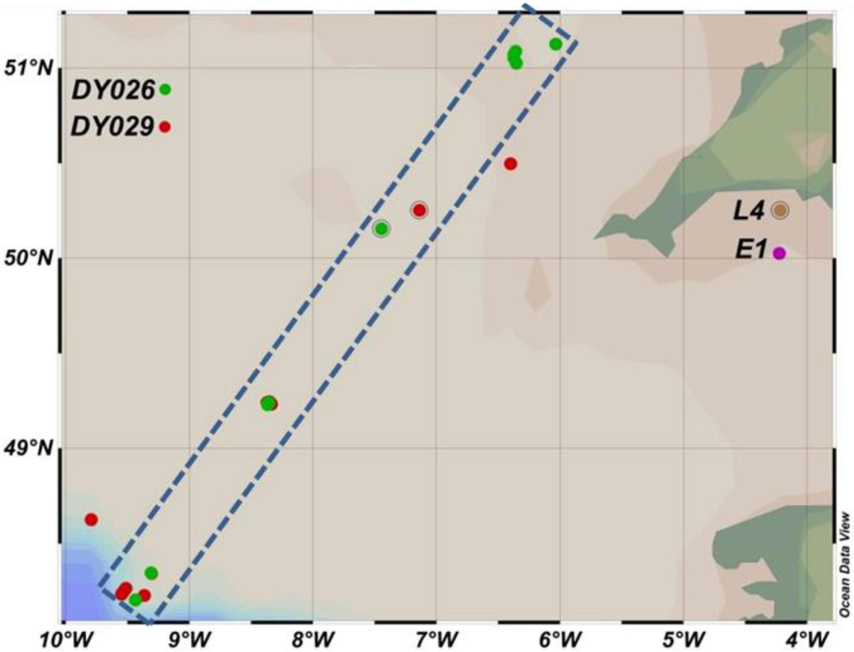
2.1. In Situ Measurements of Size Fractionated Primary Production

Water samples were collected on board Research Vessel (RV) Plymouth Quest from the Western Channel Observatory (WCO, Plymouth, England) at stations L4 and E1 between March–July 2014 and March–November 2015 (Figure 1). No data from the winter months were included. At L4, sampling depths were 0, 10, 25 and 50 m, and at E1 they were 0, 10, 30 and 60 m. Samples were also taken during two cruises to the Celtic Sea (Figure 1) during August 2014 (DY026) and April 2015 (DY029) on board Royal Research Ship (RRS) Discovery, where up to four sampling depths were chosen with respect to profiles of photosynthetically available radiation (PAR), density and fluorescence data obtained from CTD casts. PE curves were measured following the method of Tilstone et al. [70]. For each depth, 15 clear polycarbonate bottles containing 70 mL seawater were spiked with 5–10 µCi of ¹⁴C-labelled NaHCO₃ (Perkin Elmer, Buckingham, UK, administered as a 0.5–1.0 mL solution of autoclaved, 0.2 µm filtered sea water. Bottles were incubated in a linear photosynthetron and maintained at the in situ temperature. Maximum irradiance on sampling days was measured using an above-water PAR sensor (Skye Instruments, Llandrindod Wells, UK) and the maximum incubator light level in the incubator was set accordingly. High-output white LEDs were used for sampling days when maximum irradiance was <1900 µE m⁻² s⁻¹ due to their superior spectral quality and low heat output compared to incandescent bulbs. For summer sampling days with higher incident light levels, 50 W halogen bulbs were used due to their higher emission. The attenuation of PAR along the length of the incubator was accounted for by measuring PAR at each bottle position at a number of maximum irradiances. After 1.5 h incubations, each bottle was filtered through sequential 47 mm polycarbonate filters (20 µm, 2.0 µm and 0.2 µm pore sizes) as per chlorophyll samples. Each sample filter was then fumed for 15 h in 37% HCl to remove residual inorganic carbon before being placed in 6 mL vials with 4 mL scintillation cocktail (Meridian Biotech, Tadworth, UK). After 24 h in the cocktail, samples were run on a liquid scintillation counter (Tricarb—Perkin Elmer, Buckingham, UK) to determine beta particle emission. External ¹⁴C standards (Perkin Elmer, Buckingham, UK) were used to correct for quenching following the dual channel ratio method in order to generate ¹⁴C disintegrations per minute (DPM). Chlorophyll-specific photosynthesis-irradiance data were subsequently fitted to the function of Platt et al. [71] in Sigmaplot (Systat) using non-linear least squares regression as follows:

$$P^B\left(z,t\right)=P_m^B\left(z\right)\times \left(1-\exp \left(\frac{-{\alpha }^B\left(z\right)\times E_{PAR}\left(z,t\right)}{P_m^B\left(z\right)}\right)\right)\times \exp \left(\frac{-{\beta }^B\left(z\right)\times E_{PAR}\left(z,t\right)}{P_m^B\left(z\right)}\right)$$

(1)

where $P_m^B$, is the light-saturated rate of photosynthesis), α^B is the light-limited slope) and β^B is the rate of photoinhibition and E_PUR is the phytoplankton available radiation. Curves with R² ≥ 0.95 were used to determine the photo-physiological parameters $P_m^B$, ${\alpha }^B$ and β^B.

2.2. Satellite Model of Size Fractionated Primary Production

The model of Brewin et al. [68] was used to calculate daily integrated primary production (g C m⁻² d⁻¹). The model is parameterised using photosynthetic parameters and the available light [71], using depth-resolved estimates of community size structure, chlorophyll biomass and irradiance over the euphotic zone, as follows:

$$PP={{\displaystyle \int }}_{t=0}^D{{\displaystyle \int }}_{z=0}^{1.5Z_{eu}}{\displaystyle \sum }_{i=1}^3{B}_i\left(z\right)P_{m,i}^B\left(z\right)\left[1-\exp (-\frac{{\alpha }_i^B\left(z\right)E\left(z,t\right)}{P_{m,i}^B\left(z\right)})\right]dzdt$$

(2)

where $D$ is day length, $Z_{eu}$ is euphotic depth (depth of 1% of surface PAR), $z$ is depth, and $t$ is time. Subscript $i$ denotes size fraction e.g., pico (<2 µm), nano (2–20 µm), micro (>20 µm) used with respect to light-saturated $(P_{m,i}^B)$ and light-limited $\left({\alpha }_i^B\right)$ photosynthetic rate values and chlorophyll biomass ($B_i$). These size ranges are consistent with the model of Uitz et al. [35] and differ from the model of Brewin et al. [68] which defines microphytoplankton as >10 µm due to the limited concentrations of cells above 20 µm in oligotrophic Atlantic waters.

2.2.1. Estimation of Euphotic Depth

In situ data from sampling stations in the Western English Channel and cruises in the Celtic Sea were used to calculate the euphotic depth ($Z_{eu}$) at each station. Data from CTD rosette-mounted downwelling PAR sensors (Biospherical Cosine 2-pi sensor) were used to determine the depth at which downwelling PAR was 1% of surface irradiance and values of $\frac{Z}{Z_{eu}}$ were then generated for each sample depth. Measured $Z_{eu}$ and surface Chlorophyll a (Chl a) concentrations were then used to test whether $Z_{eu}$ can be estimated accurately from satellite observations of Chl a in the UK shelf using the equation of Morel, et al. [72], modified by Brewin et al [68], who used a dataset of Atlantic Ocean measurements to produce new coefficient values for the following relationship:

$$Z_{eu}={10}^{\left[q_a+q_b{\log }_{10}\left(B_s\right)+q_c{\log }_{10}{\left(B_s\right)}^2+q_d{\log }_{10}{\left(B_s\right)}^3\right]}$$

(3)

where $q_i$ are model parameters and $B_S$ is surface (or satellite-derived) chlorophyll concentration. These estimates were then compared with data collected from cruises in the Celtic and Irish Seas (JR98, CD173 [73,74]).

2.2.2. Estimation of Vertical Variability in Chlorophyll-a

Vertical biomass profiles were calculated as shifted Gaussian distributions normalised to surface Chl a following Brewin et al. [68]; see parameter $B^{B_s}$ in Equation (3). These were then applied to ocean colour surface Chl a data to reconstruct the vertical distribution of Chl a over 1.5 × $Z_{eu}$. The accuracy of the method was validated using in situ Chl a data (for stations with observations >4 depths to produce interpolated profiles). The vertical distribution of Chl a with respect to surface Chl a $\left(B^{B_s}\right)$ was calculated as follows:

$$B^{B_s}\left(\mathsf{\zeta }\right)=1-S^{B_s}\mathsf{\zeta }+B_m^{B_s}exp\left\{-{\left[\left(\mathsf{\zeta }-{\mathsf{\zeta }}_m\right)/\sigma \right]}^2\right\}$$

(4)

where $B^{B_s}$ is the Chl a profile normalised to surface concentration at dimensionless depth, $\mathsf{\zeta }$ defined as $\mathsf{\zeta }=z/Z_{eu}$, where z is geometric depth, $S^{B_s}$ is the background linear decrease of $B^{B_s}$ with increasing $\mathsf{\zeta }$, $B_m^{B_s}$ is the maximum chlorophyll concentration in the Gaussian part of the profile, ${\mathsf{\zeta }}_m$ is the dimensionless depth at which $B_m^{B_s}$ occurs and $\sigma$ is the width (in terms of $\mathsf{\zeta }$) of the $B_m^{B_s}$ peak biomass.

2.2.3. Estimation of Photosynthetic Parameters

Size-fractionated photosynthetic parameters, the light-limited slope $({\alpha }^B)$ and maximum photosynthetic rate $\left(P_m^B\right)$ measured using photosynthesis-irradiance curves made on the Celtic Sea and Western English Channel cruises were estimated as a function of dimensionless depth ($\mathsf{\zeta }$) by retuning the model of Brewin et al. [68].

Table 1. Average surface values of ${\alpha }^B$ and $P_m^B$ and their slope values $S^{Ps}$ and $S^{{\alpha }_s}$ with respect to dimensionless depth ζ for UK shelf seas data and Atlantic Ocean data following Brewin et al. [68]. Bracket values are standard deviations.

Parameter	Size Class	UK Shelf Model	Atlantic Model	Shelf Values % of Atlantic Values
$P_m^{B_s}$	Micro	4.27 (±0.25)	6.05 (±0.98)	70.6
	Nano	4.43 (±0.28)	5.13 (±0.94)	86.4
	Pico	5.51 (±0.30)	3.46 (±0.80)	159.2
${\alpha }^{B_s}$	Micro	0.050 (±0.004)	0.016 (±0.004)	312.5
	Nano	0.050 (±0.004)	0.014 (±0.003)	357.1
	Pico	0.062 (±0.004)	0.011 (±0.001)	563.6
$S^{P_s}$	Micro	0.49 (±0.09)	0.35 (±0.27)	140.0
	Nano	0.38 (±0.09)	0.59 (±0.29)	64.4
	Pico	0.45 (±0.09)	0.68 (±0.31)	66.2
$S^{{\alpha }_s}$	Micro	0.51 (±0.12)	−0.07 (±0.30)	−728.6
	Nano	0.25 (±0.12)	−0.12 (±0.23)	−208.3
	Pico	0.30 (±0.10)	−0.32 (±0.17)	−93.75

shows the mean surface values and their respective slopes with ζ for the original Atlantic Ocean parameterisation of the model, and when retuned using UK shelf sea values.

2.2.4. Estimation of Irradiance

PAR over the euphotic zone and at hourly intervals (t) over day length ($D$) (hours) were estimated from the attenuation of surface irradiance according to the sub-surface Chl a, as follows:

$$E\left(0^{-},t\right)=\frac{E_m\left(0-\right)\sin \left(\frac{\pi t}{D}\right)}{3600}$$

(5)

where $E\left(0^{-},t\right)$ is the irradiance at time t just below the surface, $E_m\left(0^{-}\right)$ is the maximum irradiance at midday just below the surface. Dividing by 3600 converts flux per hour to flux per second, for consistency with time units used in α^B (µmol m⁻² s⁻¹). For each hourly time step (t), changes with irradiance (E) with depth (z) are modelled using diffuse attenuation of PAR, thus:

$$E\left(z,t\right)=E\left(0^{-},t\right)\exp \left[-K\left(z\right)z\right]$$

(6)

where $K\left(z\right)$ is the diffuse attenuation coefficient of PAR $\left(K\right)$ at depth (z), which can vary with depth due to changes in water column optical properties. Here $K\left(z\right)$ is estimated at specific depths as a function of chlorophyll concentration $B\left(z\right)$ and background PAR attenuation coefficient $K_c$. To estimate $K\left(z\right)$, the average attenuation coefficient for the euphotic zone ($K_{Zeu})$ is first calculated as:

$$K_{Zeu}=4.6/Z_{eu}$$

(7)

where $Z_{eu}$ is the euphotic depth derived from surface Chl a and Equation (2). Next, the depth-dependent $K\left(z\right)$ was computed from the following equation from Brewin et al. [68]:

$$K\left(z\right)=\left[\left(K_{Zeu}-K_c\right)\left(\frac{B\left(z\right)}{1/N{\sum }_{j=1}^{N}Bj}\right)\right]+K_c$$

(8)

where $K_c$ denotes the background attenuation of PAR independent of phytoplankton biomass and depth—assumed to be due to pure water [75] derived from computation of K when Chl a = 0.01 mg m⁻³—and $1/N\sum _{j=1}^{N}Bj$ represents the average Chl a over the euphotic zone and beyond to 1.5$Z_{eu}$, and N is the number of depth intervals within the euphotic zone used in the computation.

2.2.5. Satellite Data

Shelf seas and open ocean variants of the model were compared against in situ data. Equation (1) requires two satellite data values per pixel in order to estimate integrated size-fractionated primary production, surface Chl a ($B_s$) and PAR. Monthly, $B_s$ for the year 2016 were taken from the Ocean-Colour Climate Change Initiative (Version 3.1, http://www.oceancolour.org/, see Sathyendranath et al. [76]), which is an error-characterised (Jackson et al. [77]) time series of merged ocean colour data from a number of satellite missions (MODIS Aqua and VIIRS for the year 2016), at approximately 4 × 4 km resolution. Note the vertical chlorophyll profile is computed from the surface concentration in the model (see Section 3.4). For PAR, monthly averages for 2016 were derived from MODIS-Aqua level-3 PAR data, extracted at 4 × 4 km resolution (https://modis.gsfc.nasa.gov/data/dataprod/ipar.php). For the open ocean variant of the model, following Brewin et al. [68], a climatology of mixed-layer depth was also used in the computation of the biomass profile (not required from the Shelf Sea model, see Section 3.4 below), from de Boyer Montégut et al. [78]. Match-ups were extracted for each month, using a 3 × 3-pixel average centered at station L4.

3. Results

3.1. Modelling Size-Fractionated Chlorophyll-a from Total Chlorophyll-a

The model of Brewin et al. [69] was used to estimate size-fractionated Chl a from total Chl a. This model was tuned to the North Atlantic, including some samples from the shelf sea (Figure 1) also used in this study. The model assumes that as total Chl a increases, the community size structure changes from picophytoplankton dominated in low-chlorophyll regions such as the gyres to microphytoplankton dominated in high-chlorophyll regions such as temperate shelf seas or upwelling zones. Nano and picophytoplankton reach asymptotic Chl a values $\left(C_n^m,C_p^m\right)$, such that $C_p$ does not increase above 0.13 mg m⁻³, and $C_n$ does not increase above 0.82 mg m⁻³, beyond which additional Chl a is apportioned to microphytoplankton. The model was retuned using observations from this study only. When compared with the Brewin et al. [69] model, the retrieved parameters were not significantly different and therefore the parameterisation of Brewin et al. [69] was used to estimate size-fractionated Chl a.

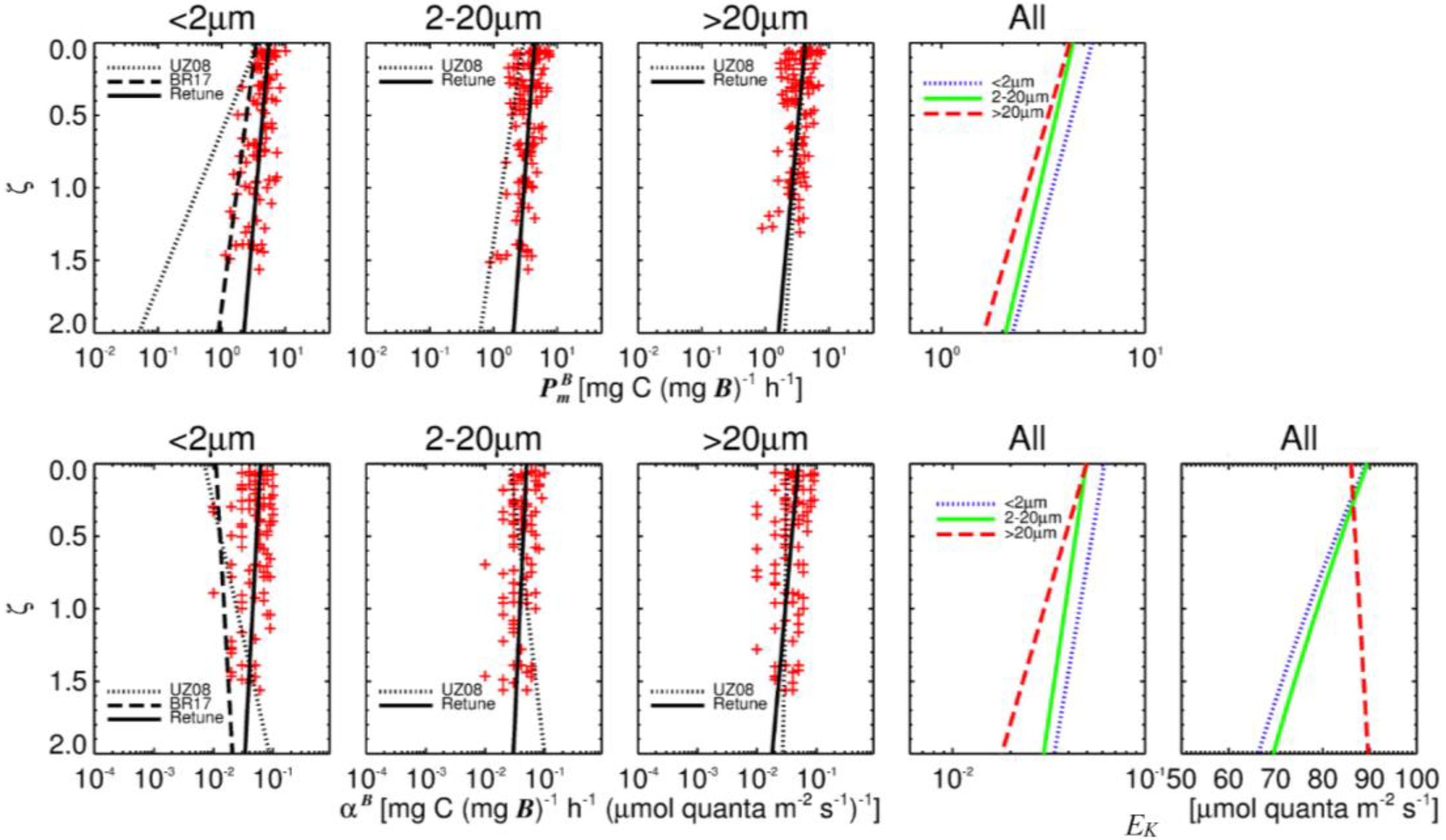
3.2. Comparison of Measured and Modelled Photosynthetic Parameters

Values of size-fractionated photosynthetic parameters with respect to the dimensionless depth ζ using the Atlantic Ocean parameterisation were compared with measured values from the UK shelf seas. Values of $P_m^B$ and ${\alpha }^B$ were modelled at specific values of ζ using:

$$P_{m,i}^B=P_{m,i}^{B_s}\exp \left(-S_i^P\zeta \right)$$

(9)

$${\alpha }_i^B={\alpha }_i^{B_s}\exp \left(-S_i^{\alpha }\zeta \right)$$

(10)

Equations (8) and (9) were used to calculate $P_m^B$ and ${\alpha }^B$ at specific dimensionless depth ζ from mean surface values $P_{m,i}^{B_s}$ and ${\alpha }_i^{B_s}$ and their respective slopes $S_i^P$ and $S_i^{\alpha }$ [68]. $P_{m,i}^{B_s}$ and ${\alpha }_i^{B_s}$ are surface values when ζ$~$0, $S_i^P$ and $S_i^{\alpha }$ are slope values quantifying the change in $P_{m,i}^B$ and ${\alpha }_i^B$ from surface values with respect to ζ. Figure 2 shows the differences between the values of $P_m^B$ and ${\alpha }^B$ estimated by both the Atlantic Ocean and Shelf seas models. Only the nano and picophytoplankton fractions can be compared, as the microphytoplankton are defined as >10 µm in the Brewin et al. [68] model whereas they are >20 µm for the Shelf seas model.

Measured values of $P_m^B$ follow a similar trend with respect to ζ compared to other models (Figure 2). However, mean measured surface values of $P_m^B$ and ${\alpha }^B$ were highest for pico and smallest for microphytoplankton, which is the opposite trend for open ocean parameterisation of the models of Uitz et al. [35] and Brewin et al. [68]. Mean measured values of $P_{m,i}^{B_s}$ and ${\alpha }_i^{B_s}$ for micro and nanophytoplankton were similar, with a higher slope for microphytoplankton causing values to decrease with increasing ζ. Picophytoplankton had significantly higher mean surface values than the larger fractions and followed a similar reduction with increasing ζ.

When compared to the profiles of Uitz et al. [35], differences in microphytoplankton photo physiology are less pronounced than for the smaller fractions, with similar mean surface values of $P_{m,i}^{B_s}$ and ${\alpha }_i^{B_s}$ and slopes $S_i^P$ and $S_i^{\alpha }$. Nano and picophytoplankton values have greater $P_{m,i}^{B_s}$ and particularly ${\alpha }_i^{B_s}$ values when compared with the values of Uitz et al. [35] and Brewin et al. [68] (pico only). Picophytoplankton values of $S_i^P$ are closer to those reported by Brewin et al. [68] while the negative values of picophytoplankton $S_i^{\alpha }$ values with ζ common to Uitz et al. [35] and Brewin et al. [68] models is not observed in the model re-tuned with UK shelf seas data. The light saturation parameter $E_k$ calculated as $(\frac{P_m^B}{{\alpha }^B})$ follows a negative trend with ζ for pico and nanophytoplankton fractions—which were of similar magnitude—while a slight positive trend is observed for microphytoplankton, which have substantially greater values of $E_k$ than smaller fractions at ζ > 0.5.

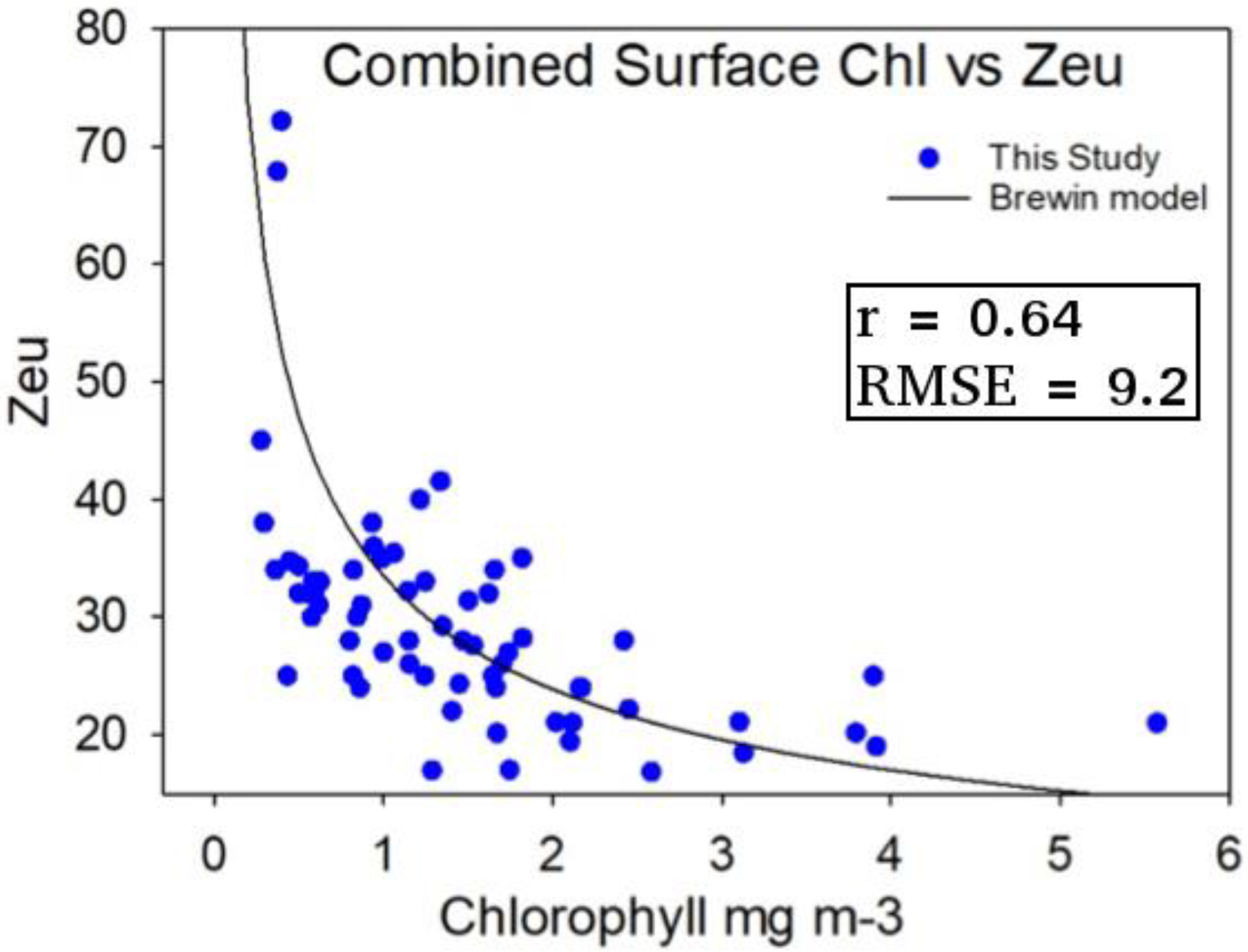
3.3. Estimation of Euphotic Depth from Surface Chlorophyll-a

Figure 3 shows measured surface chlorophyll concentrations and euphotic depth from the Western Channel and the Celtic Sea. Observations were in good agreement with the re-tuned algorithm of Brewin et al [68], though there was a considerable degree of variability at lower Chl a values (<0.7 mg m⁻³). With these results it is possible to use surface Chl a to estimate euphotic depth with some confidence, although the scatter may indicate significant concentrations of coloured dissolved organic matter (CDOM) and suspended matter (TSM) which do not co-vary with surface Chl a.

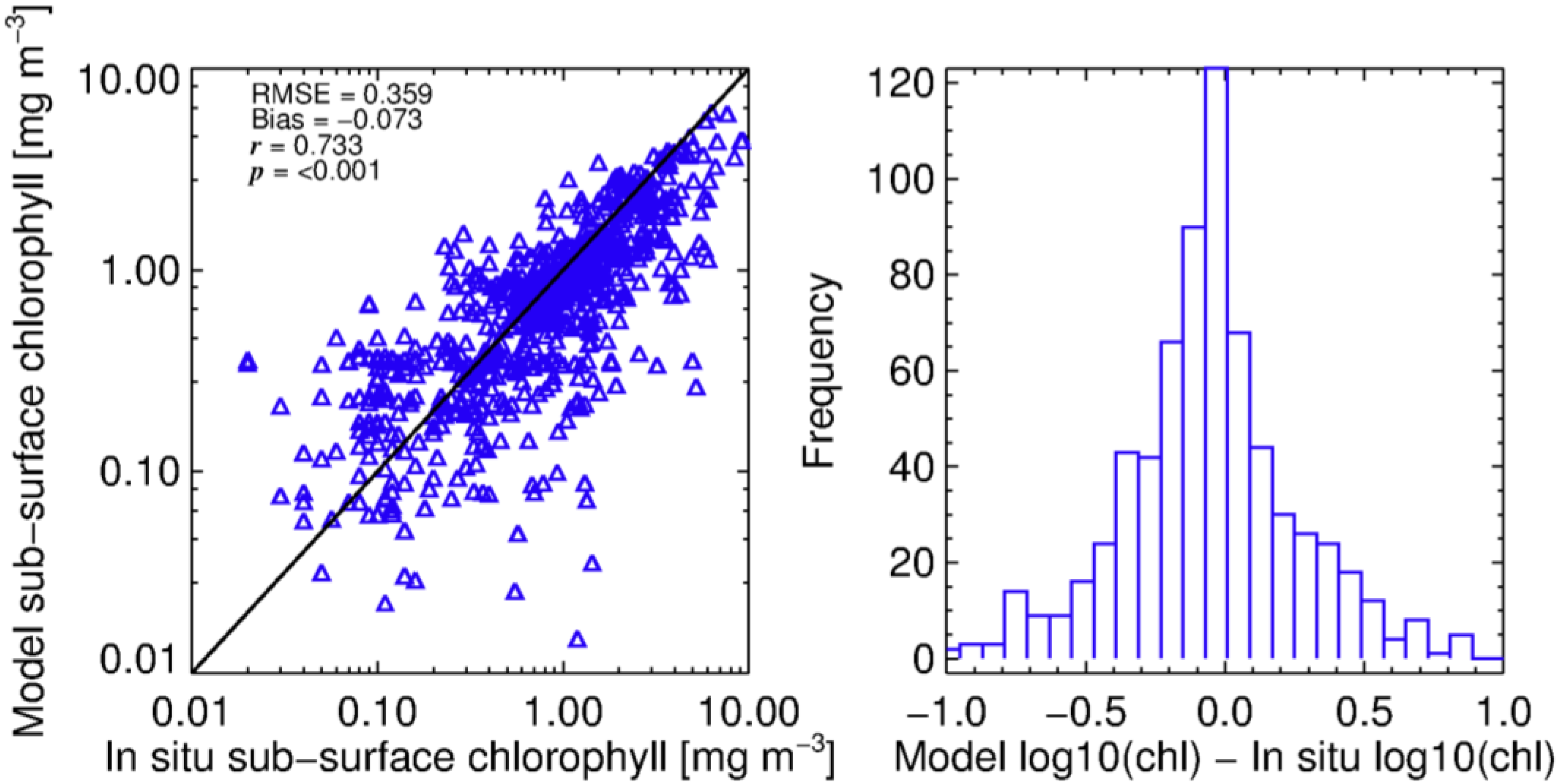
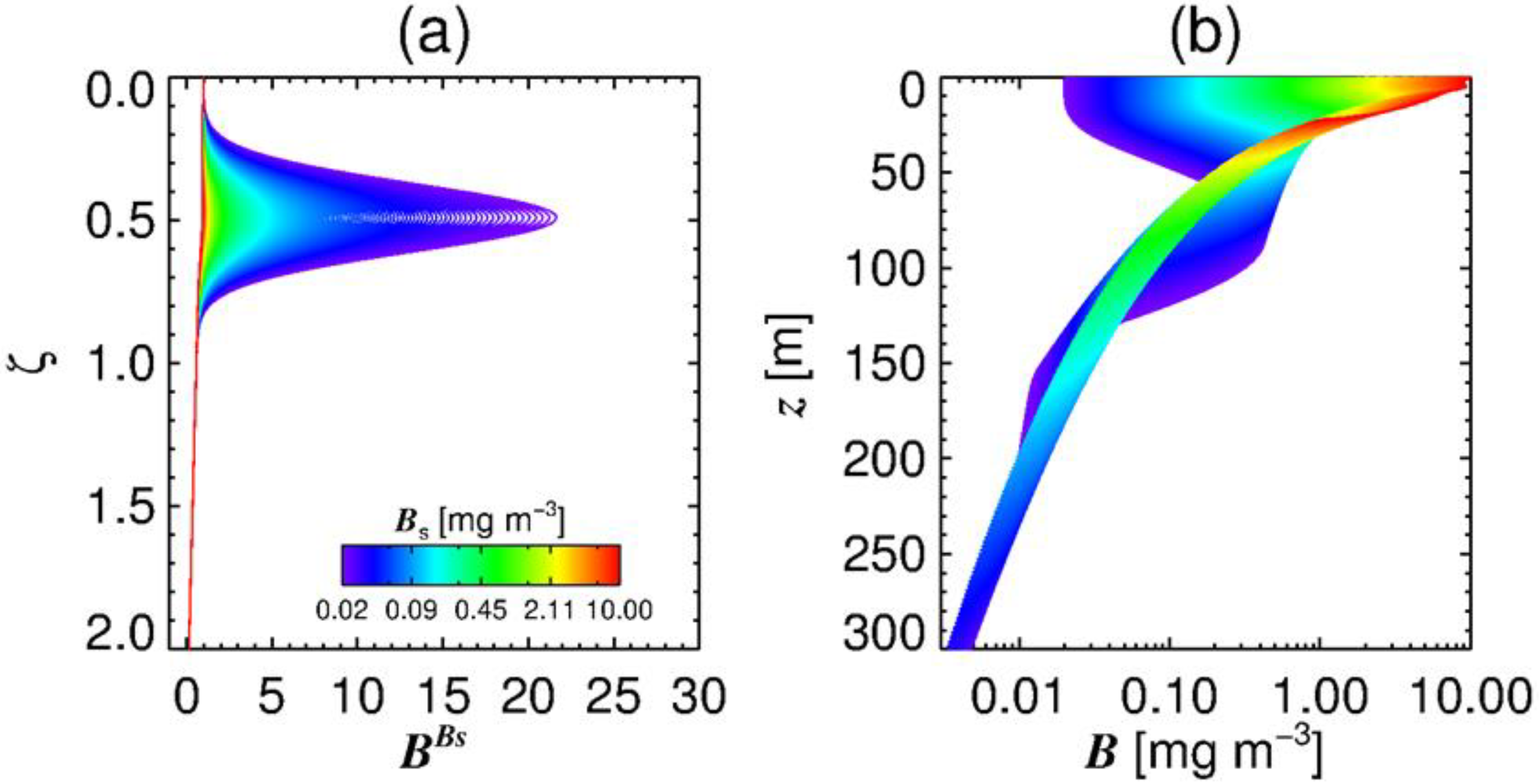
3.4. Estimation of the Vertical Distribution of Phytoplankton Biomass

Modelled sub-surface Chl a was calculated using Equation (3). Unlike the original model [68], waters were not separated into mixed and stratified conditions using the ratio of euphotic depth to mixed layer depth, then treating the mixed cases as uniform and applying Equation (3) to the stratified cases. Instead, we found a better performance when not making this partitioning and assuming Equation (3) holds for most conditions.

Figure 4 shows the improvement in model skill when making this assumption, with a Gaussian distribution in model differences. The distribution of observed versus measured values plotted via regression is more normal, with reduced bias and RMSE compared to the methods of Brewin et al. [68], indicating that this parameterisation is more representative for the Celtic Sea and Western English Channel sites from spring to summer. The derived parameters for the revised shelf model were: $S^{B_s}$ = 0.432; $B_m^{B_s}$ = ${10}^{({\log }_{10}(B_S)\times \left(-0.8\right)-0.04)}$, ${\mathsf{\zeta }}_m=0.492$; and $\sigma =0.166$.

Compared to the values reported by Brewin et al. [68], where the peak of phytoplankton biomass resides at between ζ = 0.8–1.2, Figure 5 indicates that the shelf sea data used here produce a peak biomass at shallower depths within the photic zone, though this may be due to the Case 1 light field used.

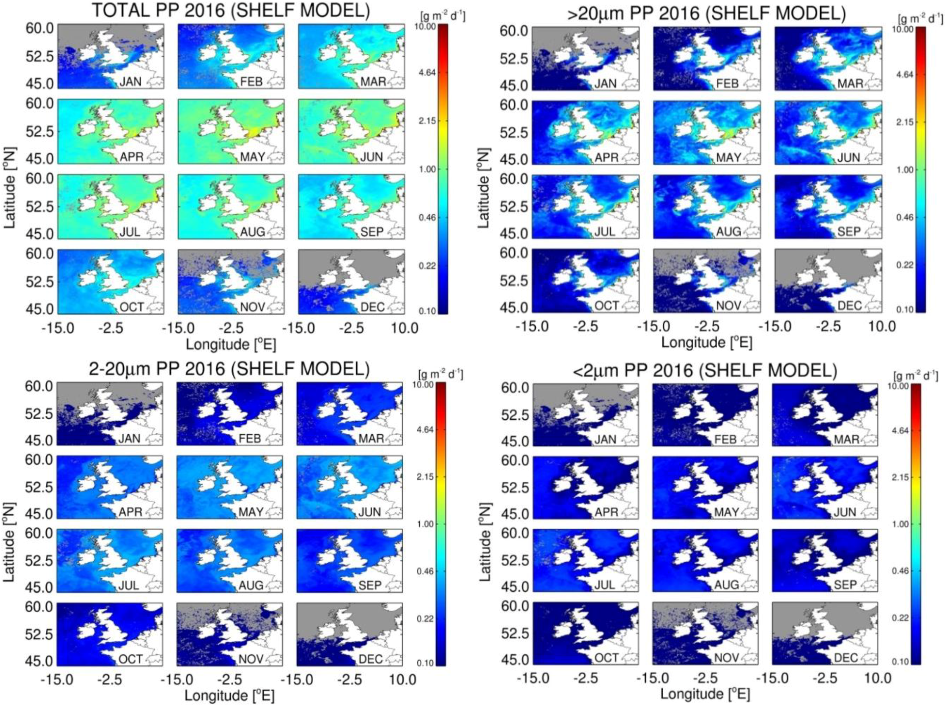
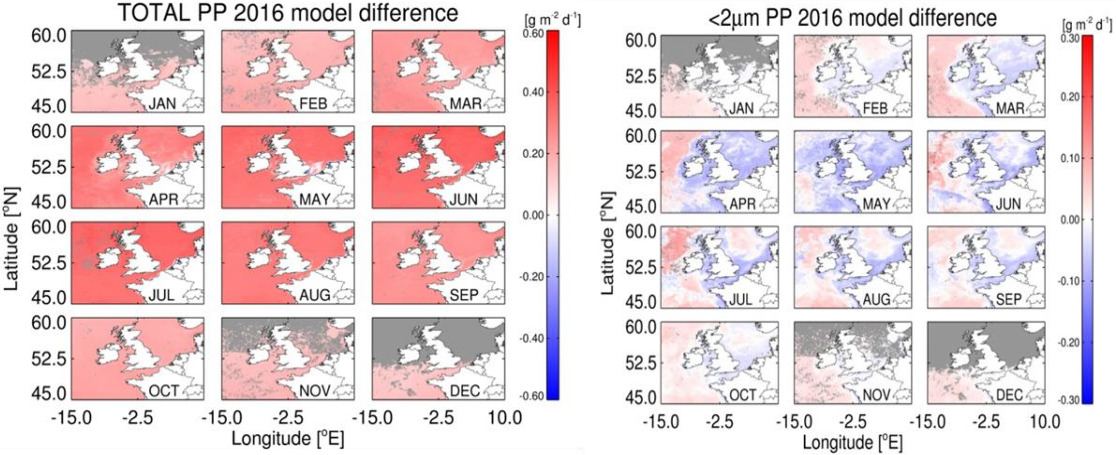
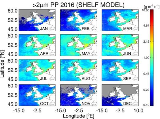
3.5. Estimates of Annual Size-Fractionated Primary Production

Using the original Atlantic Ocean (Open Sat) of Brewin et al. [68] and refined Shelf Sea (Shelf Sat) algorithms, size-fractionated primary production was estimated using remote sensing chlorophyll and PAR products for 2016, so that the results are not biased toward the shelf dataset sampled during 2014–2015. Differences between the Open and Shelf Sat models are due to the vertical profile in PE parameters for each the size-class used. Differences in model output was subsequently calculated as a positive or negative anomaly (Figure 6, Figure 7 and Figure 8), and subsequently compared with climatological means of monthly PP at the Western English Channel station L4, where a time series of total PP calculated using measured PE parameters is available.

Total daily integrated primary production form the re-tuned Shelf satellite model peaked in April (Figure 6), with open shelf regions having values of 0.6–1.7 g m⁻² d⁻¹, with the highest values of 4–6 g m⁻² d⁻¹ in estuarine regions such as the Thames estuary, The Wash, The Rhine Delta and dominated by cells >20 µm; microphytoplankton. Nanophytoplankton (2–20 µm) PP was lower and more uniformly distributed than microphytoplankton with values of 0.3–0.5 g m⁻² d⁻¹ from April–August (Figure 6), even though they have similar photosynthetic rates to microphytoplankton (Table 1). Picophytoplankton account for the lowest proportion of total PP, which never exceeds 0.4 g m⁻² d⁻¹. As they are the least abundant fraction at high Chl a, they follow an inverse pattern to microphytoplankton in the distribution of their maximal PP, with lower PP in coastal regions and often relatively higher PP in off-shelf areas.

Estimates of PP using the Shelf Sat model resulted in an increase in total PP (0.06–0.5 g m² y⁻¹) compared to the Open Sat model, with the greatest differences observed between May and July. Combined estimates of micro and nanophytoplankton PP account for the overestimation in total PP by the Shelf Sat model (Figure 8). Values in coastal regions were lower, however for the Shelf Sat model, particularly around estuarine plumes, where total PP was highest.

The difference in picophytoplankton PP between models was more complex; values of the Shelf Sat model were lower in regions of high total PP and higher in regions of low total PP (Atlantic Ocean and Northern North Sea waters) for most months. As there is considerable variability in PE parameters measured at station L4 over weekly timescales with some months being sampled less frequently through the year (

Table 2. Regression statistics for Shelf sat and Open sat models against in situ data from station L4, CCS and Off the shelf edge.

Modelled PP	r2		Slope		Intercept
	Shelf	Open	Shelf	Open	Shelf	Open
Total shelf, n = 15	0.78	0.75	0.59	0.43	321	158
Micro, Nano shelf, n = 10	0.56	0.39	0.54	0.33	309	101
Pico shelf, n = 10	0.32	0.00	0.24	-0.01	104	188

), a climatology, using average values for each month over 2009–2015, was used to compare with seasonal patterns in satellite PP to assess whether the models are able to capture the seasonal dynamics in PP. Annual trends were plotted for the original Open Sat and Shelf Sat models, and the mean climatology of measured PP. Two values of total PP were removed from the climatology for August as these were taken during a large, atypical Karenia mikimotoi bloom, but were included in Figure 9 for reference. Size-fractionated values were restricted to March–September to ensure sufficient data to calculate averages and standard error. Shelf Sat overestimated total PP compared to the climatology across all months. The Open Sat model underestimates PP from April to August and was similar to the climatological values from September to December. The Open Sat model appears more accurate during periods of lower PP, while the Shelf Sat model performs better at high values in the spring-summer period, when most of the data of this study was measured. Microphytoplankton PP estimates by the Shelf Sat model were underestimated from April–June and slightly overestimated in September, whereas values in March, July and August were similar to the measured climatological mean. Nanophytoplankton PP had considerably higher inter-annual variability than the other fractions, but satellite modelled values only fell within the climatological variability in May to June, and greatly overestimated PP outside of these months. Picophytoplankton satellite PP was closer to the climatology, except during May, August and September (Figure 9). The average seasonal dynamics of PP was generally captured for total, micro and picophytoplankton (except from August to September), but was less accurate for nanophytoplankton.

Generally, the Shelf Sat model captured the seasonal dynamics of picophytoplankton PP better between March–July, but PP values were overestimated, whereas the Open Sat model returned values closer to the climatological means. Combined micro and nanophytoplankton PP is generally better estimated by the Shelf Sat model, though is often overestimated outside of May and June. The Open Sat model consistently underestimated micro and nanophytoplankton PP.

Statistical parameters of linear regression between mean daily integrated PP values at station L4 (50.25°N, 4.21°E), Central Celtic Sea (CCS 49.24°N, 8.36°E) and off shelf (48.62°N, 9.79°E) with modelled values from the Open Sat and Shelf Sat model tunes are given in Table 2. Both models performed well for total PP, with the shelf model having a slightly higher coefficient of determination and slope closer to 1:1, but a considerable offset, consistently overestimating at low to moderate values (0–0.5 g m⁻² d⁻¹). The Open Ocean model exhibited a lower slope and offset and was more accurate at lower PP but underestimated PP at values >0.5 g m⁻² d⁻¹. The statistics indicate that the shelf model generally performs better at estimating micro + nano PP, but overestimates PP at lower values (<0.25 g m⁻² d⁻¹) which were not frequently encountered within this study. Picophytoplankton PP showed a weak correlation for the shelf model, with reduced range in PP with a tendency to underestimate PP at >0.15 g m⁻² d⁻¹. There is considerable variability in Celtic Sea PP at the same sampling sites on sub-month time scales that is not captured in monthly averages and composites. In order to calibrate and validate the Shelf Sat model to the same degree as the Open Sat model, more data from the shelf are needed, preferably sampled with match up satellite data of Chl a and PAR products.

4. Discussion

4.1. Accuracy of Size-Fractionated Primary Production Satellite Estimates for the UK Shelf Seas

By retuning the model of Brewin et al. [68] using measurements made in the Celtic Sea and Western English Channel, the overall accuracy of estimates of total and size-fractionated PP was generally improved (Figure 9 and Figure 10). The original Open Sat model provided more accurate estimates at lower PP (Figure 7), during periods of the year where no data were available to re-tune the model from the shelf seas, as in winter. Compared to in situ climatology from station L4, the Shelf Sat model overestimated PP from September to March. While the re-tuned Shelf Sea model appears to replicate the trends of PP calculated from in situ data (Figure 9 and Figure 10). There are instances however, when there are differences in the magnitude of values, with nanophytoplankton PP being greatly overestimated outside of May and June (Figure 9 and Figure 10). A sensitivity analysis of the modelled PP output was conducted by Brewin et al. [68] using Monte Carlo simulations (200 iterations) on input variables (total surface Chl a, surface irradiance and mixed layer depth) and model parameters. The sensitivity analysis of the input and parameters of the model indicated that total and size-fractionated PP were particularly sensitive to $S^{Bs}$ the background decrease of $B^{Bs}$ with ζ, and $q_a,q_b$ the empirical parameters used in the calculation of $Z_{eu}$ from surface Chl a (Equation (3)). Output PP values for nano and picophytoplankton were most sensitive to changes in asymptotic maximum Chl a $(B_1^m,B_{1,2}^m)$ and scaling parameters with respect to total Chl a $\left(S_1,S_{1,2}\right)$ in mesotrophic environments (Chl a = 0.2 mg m⁻³). There are a number of sampling stations within this study where nano- and occasionally picophytoplankton dominate size-fractionated Chl a across a range of total concentrations, meaning PP may be incorrectly apportioned to microphytoplankton when total Chl a is > 1.0 mg m⁻³. Although there were periods in this study when nanophytoplankton dominated PP, typically microphytoplankton dominated PP during spring and late summer/autumn blooms [79,80].

In the original Open Sat model, in a well-mixed eutrophic environment (Chl a = 2.0 mg m⁻³), the model is generally less sensitive to individual parameters than lower Chl a (particularly for $S^{Bs}$ as the water column is considered uniform), but the relative sensitivity to ${\alpha }_i^{B_s}$ is increased for all size fractions. Considered individually, the means by which these model parameters might be impacted in a highly seasonal, meso or eutrophic shelf sea which may explain some sources of error and elucidate ways to improve the modelling of size-fractionated PP with refined models.

4.2. Accuracy of Size-Fractionated Photosynthetic Parameters and Biomass Distribution

Total and size-fractionated PP estimates calculated by the model of Brewin et al. [68] for both the open ocean and shelf seas, are more sensitive to differences in ${\alpha }^{B_s}$ than $P_m^{B_s}$. The lower significance of $P_m^B$ as a source of error in applying this modified open ocean PP model is compounded by the smaller differences in values of $P_m^B$ and $S^{B_s}$ between the Open and Shelf Sat models than for ${\alpha }^{B_s}$ (Table 1). The parameterisation of ${\alpha }^B$ therefore has a greater impact on estimates of PP when comparing models, as there are substantial differences in ${\alpha }^{B_s}$ and $S^{{\alpha }_s}$ between each dataset (Table 1). In previous studies, ${\alpha }^B$ in shelf regions can vary over an order of magnitude, which can be due to a combination of changes in nutrients, irradiance, temperature and phytoplankton community composition [39,81,82,83,84,85]. These cannot be easily accounted for in these generalised satellite models. Differences between the Shelf Sat and in situ data may also be due to using a Case 1 light field during instances when other IOPs are significant and cCase 2 light field is required. Using cCase 1 light field will mean that Z_eu will be estimated to be deeper than it actually is if, for instance, CDOM is in higher concentrations than the Case 1 model predicts.

4.3. Effect of Hydrographic and Optical Differences on Model Performance

The sites where measurements were taken during this study ranged from shallow, coastal sites (55 m) of the English Channel, the off-shore shelf of the Celtic Sea (100–140 m) and its shelf break (200 m) to the continental slope at the Celtic Margin (1500 m). Whilst many of these areas may show similarities to North Atlantic waters [85,86,87], the hydrography and nutrient dynamics are notably different. Outside of deep winter mixing, vertical water transport in the North Atlantic is often through Ekman pumping and mesoscale eddies, with little diapycnal flux of nutrients [88,89,90]. This contrasts the NW European Shelf, where nutrients can be supplied by advective, tidal, frontal and diapycnal means, with internal tides and wind stress modifying the supply of nutrients to the euphotic layer [21,91,92,93,94,95,96,97]. There is therefore a potentially greater variability in the vertical distribution, biomass, community structure and size-fractionated photosynthesis with respect to the surface values of variables observable from satellite and their respective model parameters. For example, subsurface Chl a maxima in the seasonally stratified Celtic Sea have been observed to have greater Chl a concentrations in regions with stronger tides [96] and at higher irradiance levels and have greater nitrate supply compared to the open ocean [74,98]. Due to the difficulty in modelling variable sub-surface physical features from satellite, using simpler, generalised models of sub-surface biomass distribution tuned to the hydrography of specific regions may be a reasonable approach. The advent of combined passive ocean colour and BioArgo float arrays, offer the potential to improve the modelling of the vertical distribution of phytoplankton to increase the accuracy of satellite estimates of PP [98,99,100,101,102,103,104,105,106,107].

The Chl a algorithm used in the OC-CCI v3.1 dataset is tuned to an optical classification based on 14 optical types [77]. While it should therefore provide reliable estimates of Chl a when other optical constituents are present, the effect of the variability in light attenuation by CDOM and TSM with respect to surface Chl a is not considered in the modelling of $Z_{eu}$, as has been previously carried out in the UK shelf seas [108]. Although observed values of surface Chl a vs. $Z_{eu}$ show good overall agreement to the model being used (Figure 4), there is considerable scatter suggesting that the relationship between these two variables may be different across a shelf sea environment than in an oceanic regions due to the differences in hydrography and biogeochemistry [102,103]. As the UK shelf seas are highly heterogenous in their optical characteristics and may exhibit classical Case 1 optics in deeper, off-shore areas, to more extreme Case 2 waters around estuaries [103,104,105,106,107,108], the inclusion of IOPs in the estimation of $Z_{eu}$ may benefit the accuracy of the modelled light field from ocean colour data.The available light PP model used here is broadband, with irradiance expressed as the integrated flux of photons 400–700 nm ($\mu$mol photons m⁻² s⁻¹). It does not consider the spectral distribution of the light field and the variable specific absorption properties of phytoplankton. Future development of satellite PP models for Shelf seas should focus on a spectral irradiance approach that considers the absorption of light by CDOM and scattering of light by TSM, in order to improve estimates of PP in these environments.

Further improvements to this re-tuned model are possible, such as improving the modelling of the light field to accommodate the more coastal regions where the current model may break down. The model would also benefit from a rigorous step by step validation of each component by comparing modelled vertical structure of irradiance, size fractionated Chl-a and photosynthesis-irradiance parameters with in situ data, especially for winter where observations are lacking.

5. Conclusions

Measurements of the photosynthetic parameters, ${\alpha }^B$ and $P_m^B$, in the Celtic Sea and Western English Channel were used to re-tune a satellite model of size-fractionated PP. The model was forced with satellite surface Chl a and PAR using estimates of the vertical Chl a and photosynthetic parameters based on the in situ observations. This Shelf Sea version of the model was compared with the original parameterisation based on parameters measured in open ocean waters of the Atlantic. The Shelf Sea tuned model captured the seasonal patterns in size-fractionated PP for micro- and picophytoplankton, and generally performed better than the original open ocean model. The Shelf Seas version of the model however, substantially overestimated nanophytoplankton PP outside of May-June. The shelf-sea pigment dataset also showed a significant degree of variability in the relative concentrations of Chl a of three size fractions for a given total surface Chl a, suggesting that the relationships used to partition total chlorophyll into the three size classes from Brewin et al. [69] model may require further development for application to the UK shelf seas.

Compared to a climatology of in situ data at station L4 from 2009–2015, the Self Seas model performed better when phytoplankton biomass was high (April–August), but overestimated PP under conditions of low phytoplankton biomass. The overestimation in PP is in part due to the sensitivity of PP models to the parameterisation of the biomass profile. The difficulty in producing a generalised model of the vertical distribution of phytoplankton within the euphotic water column in seasonally-stratified shelf seas was shown to be a potential source of error in integrated estimates of daily PP, especially outside of the spring bloom period. Establishing new relationships between surface Chl a and the vertical biomass profile for UK shelf seas requires further development to improve satellite estimates of size-fractionated PP for this and similar ecosystems.

References

1. Dacey, J.W.; Wakeham, S.G. Oceanic dimethylsulfide: Production during zooplankton grazing on phytoplankton. Science 1986, 233, 1314–1316. [Google Scholar] [CrossRef] [PubMed]
2. Jin, X.; Gruber, N.; Dunne, J.; Sarmiento, J.; Armstrong, R. Diagnosing the contribution of phytoplankton functional groups to the production and export of particulate organic carbon, CaCO3, and opal from global nutrient and alkalinity distributions. Glob. Biogeochem. Cycles 2006, 20. [Google Scholar] [CrossRef]
3. Sinha, V.; Williams, J.; Meyerhöfer, M.; Riebesell, U.; Paulino, A.; Larsen, A. Air-sea fluxes of methanol, acetone, acetaldehyde, isoprene and dms from a Norwegian fjord following a phytoplankton bloom in a mesocosm experiment. Atmos. Chem. Phys. 2007, 7, 739–755. [Google Scholar] [CrossRef] [Green Version]
4. Arnold, S.; Spracklen, D.; Williams, J.; Yassaa, N.; Sciare, J.; Bonsang, B.; Gros, V.; Peeken, I.; Lewis, A.; Alvain, S. Evaluation of the global oceanic isoprene source and its impacts on marine organic carbon aerosol. Atmos. Chem. Phys. 2009, 9, 1253–1262. [Google Scholar] [CrossRef] [Green Version]
5. Pauly, D.; Christensen, V.; Guénette, S.; Pitcher, T.J.; Sumaila, U.R.; Walters, C.J.; Watson, R.; Zeller, D. Towards sustainability in world fisheries. Nature 2002, 418, 689–695. [Google Scholar] [CrossRef] [PubMed]
6. De Haas, H.; van Weering, T.C.; de Stigter, H. Organic carbon in shelf seas: Sinks or sources, processes and products. Cont. Shelf Res. 2002, 22, 691–717. [Google Scholar] [CrossRef]
7. Pace, M.; Glasser, J.; Pomeroy, L. A simulation analysis of continental shelf food webs. Mar. Biol. 1984, 82, 47–63. [Google Scholar] [CrossRef]
8. Yunev, O.A.; Carstensen, J.; Moncheva, S.; Khaliulin, A.; Ærtebjerg, G.; Nixon, S. Nutrient and phytoplankton trends on the Western Black Sea shelf in response to cultural eutrophication and climate changes. Estuar. Coast. Shelf Sci. 2007, 74, 63–76. [Google Scholar] [CrossRef]
9. McQuatters-Gollop, A.; Raitsos, D.E.; Edwards, M.; Pradhan, Y.; Mee, L.D.; Lavender, S.J.; Attrill, M.J. A long-term chlorophyll dataset reveals regime shift in North Sea phytoplankton biomass unconnected to nutrient levels. Limnol. Oceanogr. 2007, 52, 635–648. [Google Scholar] [CrossRef] [Green Version]
10. Ridgway, J.; Shimmield, G. Estuaries as repositories of historical contamination and their impact on shelf seas. Estuar. Coast. Shelf Sci. 2002, 55, 903–928. [Google Scholar] [CrossRef]
11. Gowen, R.J.; Hydes, D.; Mills, D.; Stewart, B.; Brown, J.; Gibson, C.; Shammon, T.; Allen, M.; Malcolm, S.J. Assessing trends in nutrient concentrations in coastal shelf seas: A case study in the Irish Sea. Estuar. Coast. Shelf Sci. 2002, 54, 927–939. [Google Scholar] [CrossRef]
12. Arnold, H.E.; Kerrison, P.; Steinke, M. Interacting effects of ocean acidification and warming on growth and dms-production in the haptophyte coccolithophore Emiliania huxleyi. Glob. Chang. Biol. 2013, 19, 1007–1016. [Google Scholar] [CrossRef] [PubMed]
13. Platt, T.; Rao, D.S.; Irwin, B. Photosynthesis of picoplankton in the oligotrophic ocean. Nature 1983, 301, 702–704. [Google Scholar] [CrossRef]
14. Viviani, D.A.; Björkman, K.M.; Karl, D.M.; Church, M.J. Plankton metabolism in surface waters of the tropical and subtropical Pacific Ocean. Aquat. Microb. Ecol. 2011, 62, 1–12. [Google Scholar] [CrossRef] [Green Version]
15. Montoya, J.P.; Holl, C.M.; Zehr, J.P.; Hansen, A.; Villareal, T.A.; Capone, D.G. High rates of N2 fixation by unicellular diazotrophs in the oligotrophic Pacific Ocean. Nature 2004, 430, 1027–1032. [Google Scholar] [CrossRef] [PubMed]
16. Zubkov, M.V.; Fuchs, B.M.; Tarran, G.A.; Burkill, P.H.; Amann, R. High rate of uptake of organic nitrogen compounds by prochlorococcus cyanobacteria as a key to their dominance in oligotrophic oceanic waters. Appl. Environ. Microbiol. 2003, 69, 1299–1304. [Google Scholar] [CrossRef] [PubMed]
17. Fehling, J.; Davidson, K.; Bolch, C.J.; Brand, T.D.; Narayanaswamy, B.E. The relationship between phytoplankton distribution and water column characteristics in North West European shelf sea waters. PLoS ONE 2012, 7, e34098. [Google Scholar] [CrossRef] [PubMed]
18. Edwards, M.; Richardson, A.J. Impact of climate change on marine pelagic phenology and trophic mismatch. Nature 2004, 430, 881–884. [Google Scholar] [CrossRef] [PubMed]
19. Olson, M.B.; Strom, S.L. Phytoplankton growth, microzooplankton herbivory and community structure in the southeast Bering Sea: Insight into the formation and temporal persistence of an Emiliania huxleyi bloom. Deep Sea Res. Part II Top. Stud. Oceanogr. 2002, 49, 5969–5990. [Google Scholar] [CrossRef]
20. Siemering, B.; Bresnan, E.; Painter, S.C.; Daniels, C.J.; Inall, M.; Davidson, K. Phytoplankton distribution in relation to environmental drivers on the north west european shelf sea. PLoS ONE 2016, 11, e0164482. [Google Scholar] [CrossRef] [PubMed]
21. Holligan, P. Biological implications of fronts on the northwest European continental shelf. Philos. Trans. R. Soc. Lond. A Math. Phys. Eng. Sci. 1981, 302, 547–562. [Google Scholar] [CrossRef]
22. Aumont, O.; Maier-Reimer, E.; Blain, S.; Monfray, P. An ecosystem model of the global ocean including Fe, Si, P colimitations. Glob. Biogeochem. Cycles 2003, 17. [Google Scholar] [CrossRef] [Green Version]
23. Moore, J.K.; Doney, S.C.; Kleypas, J.A.; Glover, D.M.; Fung, I.Y. An intermediate complexity marine ecosystem model for the global domain. Deep Sea Res. Part II Top. Stud. Oceanogr. 2001, 49, 403–462. [Google Scholar] [CrossRef] [Green Version]
24. Moloney, C.L.; Field, J.G. The size-based dynamics of plankton food webs. I. A simulation model of carbon and nitrogen flows. J. Plankton Res. 1991, 13, 1003–1038. [Google Scholar] [CrossRef]
25. Van den Berg, A.; Ridderinkhof, H.; Riegman, R.; Ruardij, P.; Lenhart, H. Influence of variability in water transport on phytoplankton biomass and composition in the southern North Sea: A modelling approach (fyfy). Cont. Shelf Res. 1996, 16, 907–931. [Google Scholar] [CrossRef]
26. Baretta-Bekker, J.; Baretta, J.; Ebenhöh, W. Microbial dynamics in the marine ecosystem model ersem ii with decoupled carbon assimilation and nutrient uptake. J. Sea Res. 1997, 38, 195–211. [Google Scholar] [CrossRef]
27. Finkel, Z.V.; Beardall, J.; Flynn, K.J.; Quigg, A.; Rees, T.A.V.; Raven, J.A. Phytoplankton in a changing world: Cell size and elemental stoichiometry. J. Plankton Res. 2009, 32, 119–137. [Google Scholar] [CrossRef]
28. Poulton, A.J.; Davis, C.E.; Daniels, C.J.; Mayers, K.M.J.; Harris, C.; Tarran, G.A.; Widdicombe, C.E.; Woodward, E.M.S. Seasonal phosphorus and carbon dynamics in a temperate shelf sea (Celtic Sea). Prog. Oceanogr. 2017. [Google Scholar] [CrossRef] [Green Version]
29. Arrigo, K.R. Marine microorganisms and global nutrient cycles. Nature 2004, 437, 349–355. [Google Scholar] [CrossRef] [PubMed]
30. Hessen, D.O.; Færøvig, P.J.; Andersen, T. Light, nutrients, andP:C ratios in algae: Grazer performance related to food quality and quantity. Ecology 2002, 83, 1886–1898. [Google Scholar] [CrossRef]
31. Key, T.; McCarthy, A.; Campbell, D.A.; Six, C.; Roy, S.; Finkel, Z.V. Cell size trade-offs govern light exploitation strategies in marine phytoplankton. Environ. Microbiol. 2010, 12, 95–104. [Google Scholar] [CrossRef] [PubMed]
32. Cermeno, P.; Estévez-Blanco, P.; Maranón, E.; Fernóndez, E. Maximum photosynthetic efficiency of size-fractionated phytoplankton assessed by 14C uptake and fast repetition rate fluorometry. Limnol. Oceanogr. 2005, 50, 1438–1446. [Google Scholar] [CrossRef]
33. Cermeño, P.; Marañón, E.; Rodríguez, J.; Fernández, E. Large-sized phytoplankton sustain higher carbon-specific photosynthesis than smaller cells in a coastal eutrophic ecosystem. Mar. Ecol. Prog. Ser. 2005, 297, 51–60. [Google Scholar] [CrossRef] [Green Version]
34. Maraóón, E.; Cermeóo, P.; Rodríguez, J.; Zubkov, M.V.; Harris, R.P. Scaling of phytoplankton photosynthesis and cell size in the ocean. Limnol. Oceanogr. 2007, 52, 2190–2198. [Google Scholar] [CrossRef] [Green Version]
35. Uitz, J.; Huot, Y.; Bruyant, F.; Babin, M.; Claustre, H. Relating phytoplankton photophysiological properties to community structure on large scales. Limnol. Oceanogr. 2008, 53, 614–630. [Google Scholar] [Green Version]
36. Marañón, E.; Cermeño, P.; López-Sandoval, D.C.; Rodríguez-Ramos, T.; Sobrino, C.; Huete-Ortega, M.; Blanco, J.M.; Rodríguez, J. Unimodal size scaling of phytoplankton growth and the size dependence of nutrient uptake and use. Ecol. Lett. 2013, 16, 371–379. [Google Scholar] [CrossRef] [PubMed]
37. Joint, I.; Owens, N.; Pomroy, A.; Pomeroy, A. Seasonal production of photosynthetic picoplankton and nanoplankton in the Celtic Sea. Mar. Ecol. Prog. Ser. 1986, 251–258. [Google Scholar] [CrossRef]
38. Stuart, V.; Sathyendranath, S.; Head, E.; Platt, T.; Irwin, B.; Maass, H. Bio-optical characteristics of diatom and prymnesiophyte populations in the Labrador Sea. Mar. Ecol. Prog. Ser. 2000, 201, 91–106. [Google Scholar] [CrossRef] [Green Version]
39. Morán, X.A.G.; Scharek, R. Photosynthetic parameters and primary production, with focus on large phytoplankton, in a temperate mid-shelf ecosystem. Estuar. Coast. Shelf Sci. 2015, 154, 255–263. [Google Scholar] [CrossRef] [Green Version]
40. Joint, I.; Pomroy, A. Photosynthetic characteristics of nanoplankton and picoplankton from the surface mixed layer. Mar. Biol. 1986, 92, 465–474. [Google Scholar] [CrossRef]
41. Morán, X.A.G. Annual cycle of picophytoplankton photosynthesis and growth rates in a temperate coastal ecosystem: A major contribution to carbon fluxes. Aquat. Microb. Ecol. 2007, 49, 267–279. [Google Scholar] [CrossRef]
42. Chen, Y.-L.L. Comparisons of primary productivity and phytoplankton size structure in the marginal regions of southern East China Sea. Cont. Shelf Res. 2000, 20, 437–458. [Google Scholar] [CrossRef]
43. Marañón, E.; Holligan, P.M.; Barciela, R.; González, N.; Mouriño, B.; Pazó, M.J.; Varela, M. Patterns of phytoplankton size structure and productivity in contrasting open-ocean environments. Mar. Ecol. Prog. Ser. 2001, 216, 43–56. [Google Scholar] [CrossRef] [Green Version]
44. Bricaud, A.; Claustre, H.; Ras, J.; Oubelkheir, K. Natural variability of phytoplanktonic absorption in oceanic waters: Influence of the size structure of algal populations. J. Geophys. Res. Ocean. 2004, 109. [Google Scholar] [CrossRef] [Green Version]
45. Kulk, G.; de Vries, P.; van de Poll, W.H.; Visser, R.J.; Buma, A.G. Temperature-dependent growth and photophysiology of prokaryotic and eukaryotic oceanic picophytoplankton. Mar. Ecol. Prog. Ser. 2012, 466, 43–55. [Google Scholar] [CrossRef] [Green Version]
46. Mino, Y.; Matsumura, S.; Lirdwitayaprasit, T.; Fujiki, T.; Yanagi, T.; Saino, T. Variations in phytoplankton photo-physiology and productivity in a dynamic eutrophic ecosystem: A fast repetition rate fluorometer-based study. J. Plankton Res. 2013, 36, 398–411. [Google Scholar] [CrossRef]
47. Moore, C.M.; Suggett, D.J.; Hickman, A.E.; Kim, Y.-N.; Tweddle, J.F.; Sharples, J.; Geider, R.J.; Holligan, P.M. Phytoplankton photoacclimation and photoadaptation in response to environmental gradients in a shelf sea. Limnol. Oceanogr. 2006, 51, 936–949. [Google Scholar] [CrossRef] [Green Version]
48. Banse, K. Rates of growth, respiration and photosynthesis of unicellular algae as related to cell size—A review. J. Phycol. 1976, 12, 135–140. [Google Scholar]
49. Hirata, T.; Hardman-Mountford, N.J.; Barlow, R.; Lamont, T.; Brewin, R.; Smyth, T.; Aiken, J. An inherent optical property approach to the estimation of size-specific photosynthetic rates in eastern boundary upwelling zones from satellite ocean colour: An initial assessment. Prog. Oceanogr. 2009, 83, 393–397. [Google Scholar] [CrossRef]
50. Uitz, J.; Claustre, H.; Gentili, B.; Stramski, D. Phytoplankton class-specific primary production in the world’s oceans: Seasonal and interannual variability from satellite observations. Glob. Biogeochem. Cycles 2010, 24. [Google Scholar] [CrossRef]
51. Blondeau-Patissier, D.; Gower, J.F.R.; Dekker, A.G.; Phinn, S.R.; Brando, V.E. A review of ocean color remote sensing methods and statistical techniques for the detection, mapping and analysis of phytoplankton blooms in coastal and open oceans. Prog. Oceanogr. 2014, 123, 123–144. [Google Scholar] [CrossRef] [Green Version]
52. Nair, A.; Sathyendranath, S.; Platt, T.; Morales, J.; Stuart, V.; Forget, M.-H.; Devred, E.; Bouman, H. Remote sensing of phytoplankton functional types. Remote. Sens. Environ. 2008, 112, 3366–3375. [Google Scholar] [CrossRef]
53. Alvain, S.; Moulin, C.; Dandonneau, Y.; Bréon, F.-M. Remote sensing of phytoplankton groups in case 1 waters from global SeaWiFS imagery. Deep Sea Res. Part I Oceanogr. Res. Pap. 2005, 52, 1989–2004. [Google Scholar] [CrossRef] [Green Version]
54. Astoreca, R.; Rousseau, V.; Ruddick, K.; Knechciak, C.; Van Mol, B.; Parent, J.-Y.; Lancelot, C. Development and application of an algorithm for detecting phaeocystis globosa blooms in the case 2 Southern North Sea waters. J. Plankton Res. 2008, 31, 287–300. [Google Scholar] [CrossRef] [PubMed]
55. Westberry, T.; Siegel, D.; Subramaniam, A. An improved bio-optical model for the remote sensing of trichodesmium spp. Blooms. J. Geophys. Res. Ocean. 2005, 110. [Google Scholar] [CrossRef]
56. Subramaniam, A.; Brown, C.; Hood, R.R.; Carpenter, E.; Capone, D. Detecting Trichodesmium blooms in SeaWiFS imagery. Deep Sea Res. Part II Top. Stud. Oceanogr. 2001, 49, 107–121. [Google Scholar] [CrossRef]
57. Sathyendranath, S.; Watts, L.; Devred, E.; Platt, T.; Caverhill, C.; Maass, H. Discrimination of diatoms from other phytoplankton using ocean-colour data. Mar. Ecol. Prog. Ser. 2004, 272, 59–68. [Google Scholar] [CrossRef] [Green Version]
58. Iglesias-Rodríguez, M.D.; Brown, C.W.; Doney, S.C.; Kleypas, J.; Kolber, D.; Kolber, Z.; Hayes, P.K.; Falkowski, P.G. Representing key phytoplankton functional groups in ocean carbon cycle models: Coccolithophorids. Glob. Biogeochem. Cycles 2002, 16, 47-1–47-20. [Google Scholar] [CrossRef]
59. Smyth, T.J.; Moore, G.F.; Groom, S.B.; Land, P.E.; Tyrrell, T. Optical modeling and measurements of a coccolithophore bloom. Appl. Opt. 2002, 41, 7679–7688. [Google Scholar] [CrossRef] [PubMed]
60. Carvalho, G.A.; Minnett, P.J.; Fleming, L.E.; Banzon, V.F.; Baringer, W. Satellite remote sensing of harmful algal blooms: A new multi-algorithm method for detecting the Florida Red Tide (Karenia brevis). Harmful Algae 2010, 9, 440–448. [Google Scholar] [CrossRef] [PubMed]
61. Siswanto, E.; Ishizaka, J.; Tripathy, S.C.; Miyamura, K. Detection of harmful algal blooms of Karenia mikimotoi using modis measurements: A case study of Seto-Inland Sea, Japan. Remote Sens. Environ. 2013, 129, 185–196. [Google Scholar] [CrossRef]
62. Lou, X.; Hu, C. Diurnal changes of a harmful algal bloom in the East China Sea: Observations from goci. Remote Sens. Environ. 2014, 140, 562–572. [Google Scholar] [CrossRef]
63. Saba, V.; Friedrichs, M.A.; Antoine, D.; Armstrong, R.; Asanuma, I.; Behrenfeld, M.; Ciotti, A.; Dowell, M.; Hoepffner, N.; Hyde, K.; et al. An evaluation of ocean color model estimates of marine primary productivity in coastal and pelagic regions across the globe. Biogeosciences 2011, 8, 489–503. [Google Scholar] [CrossRef] [Green Version]
64. Kutser, T. Passive optical remote sensing of cyanobacteria and other intense phytoplankton blooms in coastal and inland waters. Int. J. Remote Sens. 2009, 30, 4401–4425. [Google Scholar] [CrossRef]
65. Hunter, P.D.; Tyler, A.N.; Présing, M.; Kovács, A.W.; Preston, T. Spectral discrimination of phytoplankton colour groups: The effect of suspended particulate matter and sensor spectral resolution. Remote Sens. Environ. 2008, 112, 1527–1544. [Google Scholar] [CrossRef]
66. Bouman, H.A.; Platt, T.; Sathyendranath, S.; Li, W.K.; Stuart, V.; Fuentes-Yaco, C.; Maass, H.; Horne, E.P.; Ulloa, O.; Lutz, V.; et al. Temperature as indicator of optical properties and community structure of marine phytoplankton: Implications for remote sensing. Mar. Ecol. Prog. Ser. 2003, 258, 19–30. [Google Scholar] [CrossRef]
67. Bouman, H.; Platt, T.; Sathyendranath, S.; Stuart, V. Dependence of light-saturated photosynthesis on temperature and community structure. Deep Sea Res. Part I Oceanogr. Res. Pap. 2005, 52, 1284–1299. [Google Scholar] [CrossRef]
68. Brewin, R.J.W.; Tilstone, G.H.; Jackson, T.; Cain, T.; Miller, P.I.; Lange, P.K.; Misra, A.; Airs, R.L. Modelling size-fractionated primary production in the Atlantic Ocean from remote sensing. Prog. Oceanogr. 2017, 158, 130–149. [Google Scholar] [CrossRef]
69. Brewin, R.J.W.; Ciavatta, S.; Sathyendranath, S.; Jackson, T.; Tilstone, G.; Curran, K.; Airs, R.L.; Cummings, D.; Brotas, V.; Organelli, E.; et al. Uncertainty in ocean-color estimates of chlorophyll for phytoplankton groups. Front. Mar. Sci. 2017, 4, 104. [Google Scholar] [CrossRef]
70. Tilstone, G.H.; Figueiras, F.; Lorenzo, L.M.; Arbones, B. Phytoplankton composition, photosynthesis and primary production during different hydrographic conditions at the Northwest Iberian upwelling system. Mar. Ecol. Prog. Ser. 2003, 252, 89–104. [Google Scholar] [CrossRef] [Green Version]
71. Platt, T.; Gallegos, C.; Harrison, W. Photoinhibition of photosynthesis in natural assemblages of marine phytoplankton. J. Mar. Res. 1980, 38, 687–701. [Google Scholar]
72. Morel, A.; Huot, Y.; Gentili, B.; Werdell, P.J.; Hooker, S.B.; Franz, B.A. Examining the consistency of products derived from various ocean color sensors in open ocean (Case 1) waters in the perspective of a multi-sensor approach. Remote Sens. Environ. 2007, 111, 69–88. [Google Scholar] [CrossRef]
73. Hickman, A.E.; Holligan, P.M.; Moore, C.M.; Sharples, J.; Krivtsov, V.; Palmer, M.R. Distribution and chromatic adaptation of phytoplankton within a shelf sea thermocline. Limnol. Oceanogr. 2009, 54, 525–536. [Google Scholar] [CrossRef] [Green Version]
74. Hickman, A.E.; Moore, C.; Sharples, J.; Lucas, M.I.; Tilstone, G.H.; Krivtsov, V.; Holligan, P.M. Primary production and nitrate uptake within the seasonal thermocline of a stratified shelf sea. Mar. Ecol. Prog. Ser. 2012, 463, 39–57. [Google Scholar] [CrossRef] [Green Version]
75. Pope, R.M.; Fry, E.S. Absorption spectrum (380–700 nm) of pure water. II. Integrating cavity measurements. Appl. Opt. 1997, 36, 8710–8723. [Google Scholar] [CrossRef] [PubMed]
76. Sathyendranath, S.; Brewin, R.J.W.; Jackson, T.; Mélin, F.; Platt, T. Ocean-colour products for climate-change studies: What are their ideal characteristics? Remote Sens. Environ. 2017, 203, 125–138. [Google Scholar] [CrossRef]
77. Jackson, T.; Sathyendranath, S.; Mélin, F. An improved optical classification scheme for the Ocean Colour Essential Climate Variable and its applications. Remote Sens. Environ. 2017, 203, 152–161. [Google Scholar] [CrossRef]
78. De Boyer Montégut, C.; Madec, G.; Fischer, A.S.; Lazar, A.; Iudicone, D. Mixed layer depth over the global ocean: An examination of profile data and a profile-based climatology. J. Geophys. Res. Ocean. 2004, 109. [Google Scholar] [CrossRef] [Green Version]
79. Sathyendranath, S.; Cota, G.; Stuart, V.; Maass, H.; Platt, T. Remote sensing of phytoplankton pigments: A comparison of empirical and theoretical approaches. Int. J. Remote. Sens. 2001, 22, 249–273. [Google Scholar] [CrossRef]
80. Widdicombe, C.E.; Eloire, D.; Harbour, D.; Harris, R.P.; Somerfield, P.J. Long-term phytoplankton community dynamics in the western english channel. J. Plankton Res. 2010, 32, 643–655. [Google Scholar] [CrossRef]
81. Wiltshire, K.H.; Malzahn, A.M.; Wirtz, K.; Greve, W.; Janisch, S.; Mangelsdorf, P.; Manly, B.F.; Boersma, M. Resilience of North Sea phytoplankton spring bloom dynamics: An analysis of long-term data at Helgoland roads. Limnol. Oceanogr. 2008, 53, 1294–1302. [Google Scholar] [CrossRef]
82. De Madariaga, I.; Joint, I. Photosynthesis and carbon metabolism by size-fractionated phytoplankton in the southern North Sea in early summer. Cont. Shelf Res. 1994, 14, 295–311. [Google Scholar] [CrossRef]
83. Barnes, M.K.; Tilstone, G.H.; Suggett, D.J.; Widdicombe, C.E.; Bruun, J.; Martinez-Vicente, V.; Smyth, T.J. Temporal variability in total, micro-and nano-phytoplankton primary production at a coastal site in the western English Channel. Prog. Oceanogr. 2015, 137, 470–483. [Google Scholar] [CrossRef]
84. Segura, V.; Lutz, V.A.; Dogliotti, A.; Silva, R.I.; Negri, R.M.; Akselman, R.; Benavides, H. Phytoplankton types and primary production in the Argentine Sea. Mar. Ecol. Prog. Ser. 2013, 491, 15–31. [Google Scholar] [CrossRef]
85. Pemberton, K.; Rees, A.P.; Miller, P.I.; Raine, R.; Joint, I. The influence of water body characteristics on phytoplankton diversity and production in the Celtic Sea. Cont. Shelf Res. 2004, 24, 2011–2028. [Google Scholar] [CrossRef]
86. Birchill, A.J.; Milne, A.; Woodward, E.M.S.; Harris, C.; Annett, A.; Rusiecka, D.; Achterberg, E.P.; Gledhill, M.; Ussher, S.J.; Worsfold, P.J.; et al. Seasonal iron depletion in temperate shelf seas. Geophys. Res. Lett. 2017, 44, 8987–8996. [Google Scholar] [CrossRef] [Green Version]
87. Holligan, P.; Groom, S. Phytoplankton distributions along the shelf break. Proc. R. Soc. Edinb. Sect. B Biol. Sci. 1986, 88, 239–263. [Google Scholar] [CrossRef]
88. Martin, A.P.; Richards, K.J. Mechanisms for vertical nutrient transport within a North Atlantic mesoscale eddy. Deep Sea Res. Part II Top. Stud. Oceanogr. 2001, 48, 757–773. [Google Scholar] [CrossRef]
89. Williams, R.G.; Follows, M.J. The Ekman transfer of nutrients and maintenance of new production over the North Atlantic. Deep Sea Res. Part I Oceanogr. Res. Pap. 1998, 45, 461–489. [Google Scholar] [CrossRef]
90. McGillicuddy, D.; Anderson, L.; Doney, S.; Maltrud, M. Eddy-driven sources and sinks of nutrients in the upper ocean: Results from a 0.1 resolution model of the North Atlantic. Glob. Biogeochem. Cycles 2003, 17. [Google Scholar] [CrossRef]
91. Palmer, M.R.; Stephenson, G.R.; Inall, M.E.; Balfour, C.; Düsterhus, A.; Green, J.A.M. Turbulence and mixing by internal waves in the Celtic Sea determined from ocean glider microstructure measurements. J. Mar. Syst. 2015, 144, 57–69. [Google Scholar] [CrossRef] [Green Version]
92. Palmer, M.; Green, M.; Inall, M.; Hopkins, J. Internal tidal bores and turbulent mixing at the Celtic Sea shelf break. In Proceedings of the AGU Fall Meeting Abstracts, San Francisco, CA, USA, 3–7 December 2012. [Google Scholar]
93. Sharples, J.; Tett, P. Modelling the effect of physical variability on the midwater chlorophyll maximum. J. Mar. Res. 1994, 52, 219–238. [Google Scholar] [CrossRef]
94. Tweddle, J.F.; Sharples, J.; Palmer, M.R.; Davidson, K.; McNeill, S. Enhanced nutrient fluxes at the shelf sea seasonal thermocline caused by stratified flow over a bank. Prog. Oceanogr. 2013, 117, 37–47. [Google Scholar] [CrossRef] [Green Version]
95. Green, J.M.; Simpson, J.H.; Legg, S.; Palmer, M.R. Internal waves, baroclinic energy fluxes and mixing at the European shelf edge. Cont. Shelf Res. 2008, 28, 937–950. [Google Scholar] [CrossRef]
96. Pingree, R.D.; Mardell, G.T.; Holligan, P.M.; Griffiths, D.K.; Smithers, J. Celtic Sea and Armorican current structure and the vertical distributions of temperature and chlorophyll. Cont. Shelf Res. 1982, 1, 99–116. [Google Scholar] [CrossRef]
97. Pérez, V.; Fernández, E.; Marañón, E.; Morán, X.A.G.; Zubkov, M.V. Vertical distribution of phytoplankton biomass, production and growth in the Atlantic subtropical gyres. Deep Sea Res. I 2006, 53, 1616–1634. [Google Scholar]
98. Reul, A.; Rodríguez, J.; Blanco, J.; Rees, A.; Burkill, P. Control of microplankton size structure in contrasting water columns of the Celtic Sea. J. Plankton Res. 2006, 28, 449–457. [Google Scholar] [CrossRef] [Green Version]
99. Schulien, J.A.; Behrenfeld, M.J.; Hair, J.W.; Hostetler, C.A.; Twardowski, M.S. Vertically-resolved phytoplankton carbon and net primary production from a high spectral resolution lidar. Opt. Express 2017, 25, 13577–13587. [Google Scholar] [CrossRef] [PubMed]
100. Hu, Y.; Behrenfeld, M.; Hostetler, C.; Pelon, J.; Trepte, C.; Hair, J.; Slade, W.; Cetinic, I.; Vaughan, M.; Lu, X. Ocean lidar measurements of beam attenuation and a roadmap to accurate phytoplankton biomass estimates. In Proceedings of the EPJ Web of Conferences, Thessaloniki, Greece, 29 August–3 September 2016. [Google Scholar]
101. Hostetler, C.A.; Behrenfeld, M.J.; Hu, Y.; Hair, J.W.; Schulien, J.A. Spaceborne lidar in the study of marine systems. Annu. Rev. Mar. Sci. 2017, 10, 121–147. [Google Scholar] [CrossRef] [PubMed]
102. Tilstone, G.H.; Smyth, T.J.; Gowen, R.J.; Martinez-Vicente, V.; Groom, S.B. Inherent optical properties of the Irish Sea and their effect on satellite primary production algorithms. J. Plankton Res. 2005, 27, 1–22. [Google Scholar] [CrossRef]
103. Siegel, D.; Maritorena, S.; Nelson, N.; Behrenfeld, M.; McClain, C. Colored dissolved organic matter and its influence on the satellite-based characterization of the ocean biosphere. Geophys. Res. Lett. 2005, 32. [Google Scholar] [CrossRef] [Green Version]
104. Nelson, N.B.; Siegel, D.A. The global distribution and dynamics of chromophoric dissolved organic matter. Annu. Rev. Mar. Sci. 2013, 5, 447–476. [Google Scholar] [CrossRef] [PubMed]
105. Kratzer, S.; Bowers, D.; Tett, P. Seasonal changes in colour ratios and optically active constituents in the optical Case-2 waters of the Menai Strait, North Wales. Int. J. Remote Sens. 2000, 21, 2225–2246. [Google Scholar] [CrossRef]
106. International Ocean-Colour Coordinating Group (IOCCG). Remote Sensing of Ocean Colour in Coastal and Other Optically-Complex Waters; IOCCG Report; IOCCG: Dartmouth, Germany, 2000; 137p. [Google Scholar]
107. Groom, S.; Martinez-Vicente, V.; Fishwick, J.; Tilstone, G.; Moore, G.; Smyth, T.; Harbour, D. The western English Channel observatory: Optical characteristics of station L4. J. Mar. Syst. 2009, 77, 278–295. [Google Scholar] [CrossRef]
108. Astoreca, R.; Rousseau, V.; Lancelot, C. Coloured dissolved organic matter (CDOM) in Southern North Sea waters: Optical characterization and possible origin. Estuar. Coast. Shelf Sci. 2009, 85, 633–640. [Google Scholar] [CrossRef]
Figure 1. Sampling sites of Western English Channel and Celtic Sea. Green points are autumn campaign; Red points are summer campaign. Dotted box shows transect between Central Celtic Sea (CCS) stations (49–51.5° N) and off-shelf (48–49° N). L4 and E1 are the Western English Channel time series stations.
Remotesensing 10 01389 g001
Figure 2. Relationship of P m B and α B with respect to ζ for each size class using the retuned shelf model (black lines) with the models of Uitz et al. [35] (dotted lines) and Brewin et al. [68] (dashed lines). Values for light saturation parameter E k of retuned model in bottom right panel.
Remotesensing 10 01389 g002
Figure 3. In situ measurements of surface Chl a and Z e u measured in the Western English Channel and Celtic Sea during four separate cruises (DY026, DY029, JR98, CD173) [72,73]. Equation (3) from the model of Brewin et al. [68] is overlaid (black line) to indicate differences with the measured shelf sea data. r is the correlation coefficient between Z e u   estimates from the Brewin et al. [68] model and the data, and RMSE is the root mean square difference in meters, between the model and data.
Remotesensing 10 01389 g003
Figure 4. Modelled Chl a calculated using Equation (3) assuming a stratified water column vs. profiles of in situ measurements of chlorophyll from UK shelf seas. Statistical tests were performed in log10 space.
Remotesensing 10 01389 g004
Figure 5. In (a) it shows the relative biomass ( B B s ) with respect to dimensionless depth (ζ) and surface chlorophyll concentration ( B s ) , and (b) shows the absolute concentration of chlorophyll-a at specific depths across a range of surface chlorophyll values. Note that the x-axis is normalised to surface Chl a.
Remotesensing 10 01389 g005
Figure 6. Estimates of total and size-fractionated primary production (PP) using the retuned shelf model run with the monthly composites of European Space Agency (ESA) Ocean Colour Climate Change Intiative (OC-CCI) Chl a product data and NASA MODIS-Aqua photosynthetically available radiation (PAR).
Remotesensing 10 01389 g006
Figure 7. Differences in total and <2 µm PP using the Shelf Sat and Open Sat models.
Remotesensing 10 01389 g007
Figure 8. Estimates of monthly micro + nanophytoplankton PP using the Shelf Sat model (left panel) and the difference in micro + nanophytoplankton PP estimated by the Shelf Sat and Open Sat models (right panel).
Remotesensing 10 01389 g008
Figure 9. Climatological means of measured total and size-fractionated PP for station L4 2009–2015 with standard error and the Shelf Sat model for 2016.
Remotesensing 10 01389 g009
Figure 10. Climatological means of picophytoplankton and micro + nanophytoplankton PP for station L4 2009–2015 with standard error plotted with estimates by the Shelf Sat and Open Sat models using OC-CCI v3.1 chlorophyll imagery for 2016.
Remotesensing 10 01389 g010