Article

ERN: Edge Loss Reinforced Semantic Segmentation Network for Remote Sensing Images

1
School of Electronic and Information Engineering, Beihang University, Beijing 100191, China
2
Unmanned Systems Research Institute, Beihang University, Beijing 100191, China
*
Author to whom correspondence should be addressed.
Remote Sens. 2018, 10(9), 1339; https://doi.org/10.3390/rs10091339
Submission received: 7 July 2018 / Revised: 14 August 2018 / Accepted: 14 August 2018 / Published: 22 August 2018
(This article belongs to the Special Issue Robust Multispectral/Hyperspectral Image Analysis and Classification)

Abstract

:
The semantic segmentation of remote sensing images faces two major challenges: high inter-class similarity and interference from ubiquitous shadows. In order to address these issues, we develop a novel edge loss reinforced semantic segmentation network (ERN) that leverages the spatial boundary context to reduce the semantic ambiguity. The main contributions of this paper are as follows: (1) we propose a novel end-to-end semantic segmentation network for remote sensing, which involves multiple weighted edge supervisions to retain spatial boundary information; (2) the main representations of the network are shared between the edge loss reinforced structures and semantic segmentation, which means that the ERN simultaneously achieves semantic segmentation and edge detection without significantly increasing the model complexity; and (3) we explore and discuss different ERN schemes to guide the design of future networks. Extensive experimental results on two remote sensing datasets demonstrate the effectiveness of our approach both in quantitative and qualitative evaluation. Specifically, the semantic segmentation performance in shadow-affected regions is significantly improved.

1. Introduction

With the rapid development of remote sensing, it has become much easier to obtain high-resolution images [1,2,3]. The ever-increasing amount of data places more emphasis on automated interpretation of remote sensing images [2,4]. As an important step towards scene understanding [5], segmentation plays a vital role in many important remote sensing applications [6], such as natural hazards detection [7], urban planning [8,9], land cover mapping [10] and so on. Unlike the classical paradigm in geographic object-based image analysis that unsupervised segmentation is followed by classification [11,12,13,14], semantic segmentation employs a pixel-level supervised style and assigns each pixel with a pre-designed label.
Recently, deep convolutional neural network (CNN)-based semantic segmentation has drawn a great deal of attention due to excellent performances [15,16]. In particular, the encoder–decoder architecture has been proven highly effective in generating pixel-wise predictions in an end-to-end style [17,18,19]. Despite this success, some detail is lost after down-sampling during the encoder forward stage, which means that predictions tend to be less accurate near boundaries [20,21]. A typical idea is to add skip connections that assemble high-resolution feature maps from the encoder to learn a more precise output [22]. For remote sensing images, Volpi et al. [23] proposed a full patch labeling (FPL) network to up-sample the rough spatial maps with successive deconvolution layers. Liu et al. [24] proposed an hourglass-shaped network (HSNet) and replaced some convolution layers with inception and residual blocks to further enhance the ability of context information extraction.
Even though the above works have achieved remarkable progress, semantic segmentation for remote sensing images is far from being solved and remains a challenging task due to the complex surface environments. The inter-class variance of different surface types in remote sensing images is extremely low, which makes accurate labeling near boundaries difficult. For example, the buildings and surfaces in Figure 1a present a very similar visual appearance that confuses the network. In addition, the ubiquitous shadows in remote sensing images further decrease the inter-class variance, resulting in a large amount of semantic ambiguity and intensifying the challenge of semantic segmentation. Figure 1b shows the incorrect labeling under the interference of shadows.
Typical semantic segmentation approaches mainly focus on mitigating semantic ambiguity via providing rich information [19,24]. However, redundant and noisy semantic information from high-resolution feature maps may clutter the final pixel-wise predictions [25]. Consideration of which kind of information can directly help the network to better distinguish different semantics is needed. The boundary information is simple but effective to indicate the semantic separation between different regions. In fact, the traditional high-order conditional random field (CRF) based semantic segmentation methods utilize superpixels to retain boundary information [26,27]. There are also some superpixel-based CNN models for semantic segmentation [15,28]. Their main shortcoming is that the superpixel is unlearnable and not robust. Thanks to the holistically-nested edge detection (HED) network [29], deep net-style edges have shown the capacity to improve the performance of high-level semantic tasks [30,31]. Chen et al. [32] proposed an edge-preserving filtering method using domain transform to enhance object localization accuracy in semantic segmentation. Cheng et al. [33] fused semantic segmentation net and edge net with a regularization method to refine entire network. Marmanis et al. [34] proposed a model that cascades the edge net (HED [29]) and semantic segmentation net (FCN [17]/SegNet [19]), where the model is complex and the training phase must be carefully fine-tuned. In contrast to these works, we sought to establish a simple and scalable model that integrates multiple weighted edge structures into semantic segmentation.
To this end, this paper proposes a novel edge loss reinforced semantic segmentation network (ERN). The framework follows the encoder–decoder architecture shown in Figure 2. The edge loss reinforced structures are constructed at the encoder and decoder parts, which consist of convolution layers and an edge ground truth supervision (only in the training phase). ERN leverages the edge loss reinforced structures to focus on the low-level boundary features and further reduce semantic ambiguity. It should be noted that the edge ground truth is obtained by a simple calculation of the semantic ground truth gradient, which does not require extra manual labeling effort.
The main contributions of our paper are as follows: (1) we propose a novel edge loss reinforced semantic segmentation network for remote sensing. By introducing multiple weighted edge supervisions, the network can better preserve the spatial boundary information and significantly improve semantic segmentation performance; (2) the main representations of the network are shared between the edge loss reinforced structures and semantic segmentation, which means that the ERN simultaneously achieves semantic segmentation and edge detection without significantly increasing the model complexity; and (3) different ERN schemes are explored and discussed to provide guidelines for applying edge loss reinforced structures to future networks.
We evaluate the performance of ERN on two remote sensing datasets: (1) UAV (unmanned aerial vehicle) Image Dataset, which is collected by a medium-altitude UAV; and the (2) ISPRS Vaihingen Dataset [35], which is a publicly available dataset for 2D semantic labeling. Experimental results show that our ERN achieved a performance that excelled the referenced methods and was significantly improved for regions near the boundary or in shadow. The remainder of the paper is organized as follows. In Section 2, we review recent related literature. We describe the ERN architecture in Section 3. In Section 4, we design the experiments and compare the performance of ERN with several CNN-based baselines. Section 5 discusses experimental results and the limitation of ERN, as well as future research directions. In addition, Section 6 gives a brief statement of our work.

2. Background

Semantic segmentation is one of the key problems in the field of computer vision [36]. In contrast to classification and recognition tasks [37,38,39], which outputs one label for the whole image, semantic segmentation assigns a pre-designed label to each pixel in an image and is thus also called pixel-wise labeling. We found that different pixel-wise labeling tasks share similar principles and frameworks. We first introduce the semantic segmentation models and then briefly present some related pixel-wise labeling methods.
Semantic segmentation models. Before the widespread application of CNN-based architectures, one kind of successful traditional method formulated semantic segmentation as a CRF-based energy minimization problem [26,27]. The expression for energy consists of a unary energy term, a pairwise energy term, and a superpixel-based high-order energy term. The superpixels are usually obtained by bottom-up image segmentation methods [40,41,42], which include a large amount of image boundary information. Our work is partly inspired by the idea that retaining the boundary information can help to establish spatial context constraints. Since they were limited by the ability of hand-crafted features [43], traditional CRF based methods were gradually surpassed by CNN-based architectures.
A fully convolutional network [17] was proposed where the fully connected layers of classification models [37,44] were replaced with deconvolution layers to produce dense pixel-wise predictions, demonstrating how CNNs can be trained end-to-end for semantic segmentation. However, deconvolutional layers produce coarse segmentation maps because of a loss of information during pooling. Two different classes of architectures have evolved in the literature to tackle this issue. The first strengthens the power of the decoder part, in which skip connections from the encoder to the decoder, along with gradual deconvolution, help to more effectively recover details [19,22,24]. Apart from the above architecture, another insightful work came from dilated/à-trous convolutions [45,46,47,48], which support exponentially expanding receptive fields without losing resolution. In addition, CRF has been applied to refine the semantic segmentation results [46,47,49,50].
Related models. From a broader perspective, edge detection, salient object detection, and object symmetry detection can all be regarded as pixel labeling problems. The difference between them is that their label value spaces are different, including “edge” or “non-edge”, “object” or “non-object”.
The HED [29] comprises a single-stream deep network with multiple side outputs. Each side-output layer is also associated with a classifier to perform deep layer supervision to "guide" early classification results, as in [51]. Thus, the loss of HED consists of side output loss and fuse loss. Hou et al. [52] further propose a deeply supervised salient object detection method (DSS) by introducing short connections to the skip-layer structures within the HED architecture. Ke et al. [53] propose a side-output residual network (SRN) for symmetry detection based on HED architecture. SRN leverages output residual units (RUs) to fit the errors between side outputs and ground truth. The short connection in DSS and residual units in SRN is extremely similar.
The above literature shows a strong correlation between different pixel labeling tasks. The network for one task can be applied to other tasks with slight or even no modification. Therefore, we were inspired to combine semantic segmentation with edge detection in a single network in which the edge outputs are deeply supervised within additional edge loss reinforced structures.

3. Proposed Edge Loss Reinforced Semantic Segmentation Network
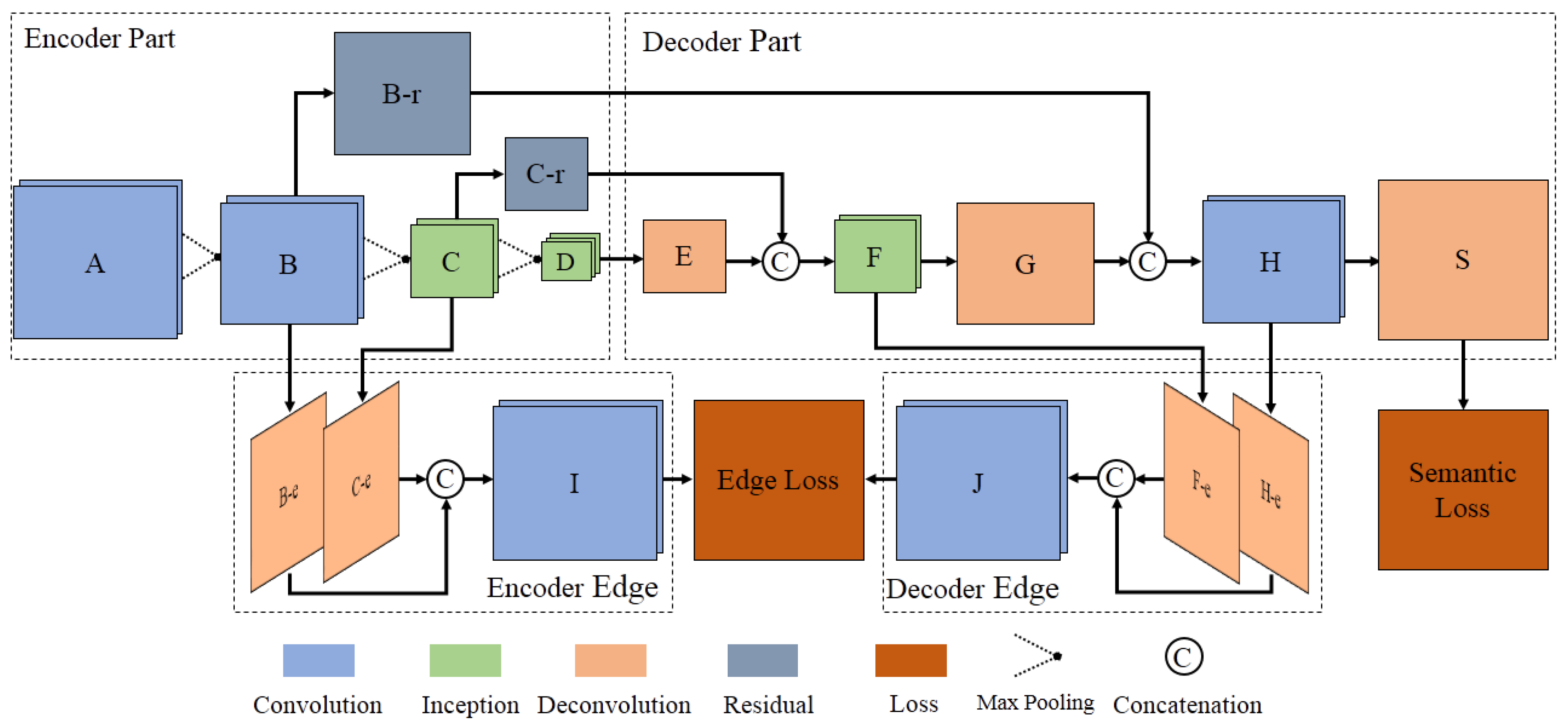
3.1. Model Overview

Our proposed ERN model is illustrated in Figure 2 and Figure 3. ERN consists of an encoder–decoder semantic segmentation net with two additional edge loss reinforced structures constructed from encoder and decoder parts, respectively. The corresponding semantic loss and edge loss are jointly trained end-to-end in order to optimize the process.
The first component is an encoder–decoder semantic segmentation net based on the HSNet [24]. The encoder part includes convolution layers, inception blocks [54], and max pooling layers. The spatial resolution of feature maps gradually decreases after pooling. The decoder part mainly includes deconvolution layers and inception blocks. The deconvolution is used to progressively up-sample the feature maps to the original spatial resolution of the input images. The skip connections from the encoder to the decoder use residual blocks [44].
The second component is the edge loss reinforced structures. Feature maps with different spatial resolution (e.g., after convolution layer H and inception block F) are directly deconvoluted to the original input size and then concatenated to further produce edge predictions. The edge loss reinforced structure is supervised by the edge ground truth. The configurations of ERN are listed in Table 1, which lists the kernel size, output number, and spatial resolution of each layer. The configurations of inception blocks (C, D, and F) and residual blocks (B-r and C-r) are discussed in Section 3.3.

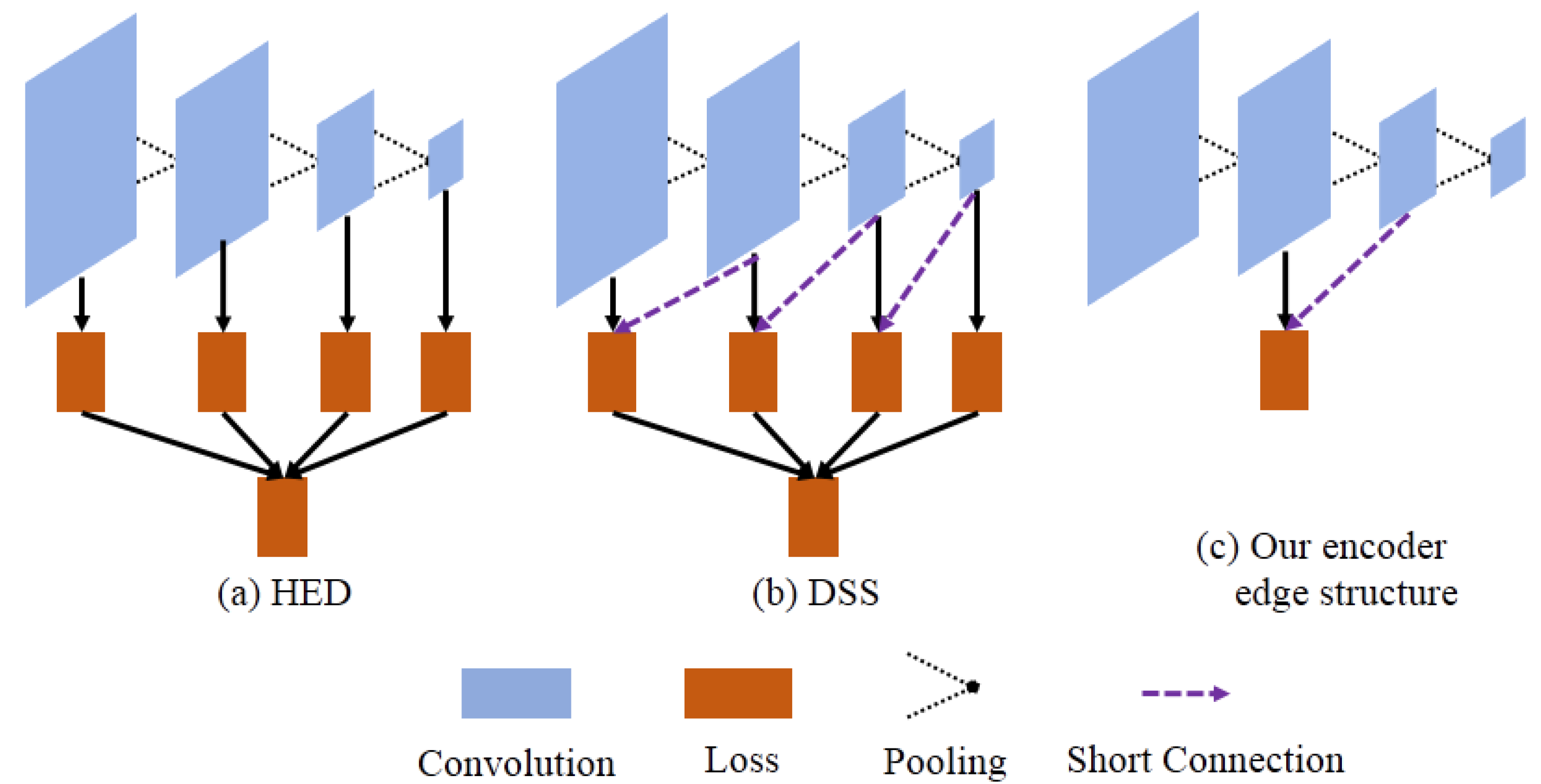
3.2. The Edge Loss Reinforced Structure Based on Short Connection

The edge loss reinforced structure in ERN was inspired by HED [29] and DSS [52]. Different architectures are illustrated in Figure 4. Figure 4a shows a simplified version of HED, showing the proposed scheme with deep supervision for each side output and fuse output. Thus, a series of side losses are added after each side output to preserve more detailed edge information. DSS further connects feature maps at different scales before output, as shown in Figure 4b.
HED [29] and DSS [52] were designed to accomplish one specific task. However, the edge loss reinforced structure within ERN is auxiliary to the semantic segmentation. It was designed to be as simple as possible, to balance the trade-off between edge detection performance and model complexity. Therefore, we simplify the edge loss reinforced structure so that the entire model is not too complicated. Moreover, the lower-resolution feature map has poorer spatial accuracy because of pooling operations, as discussed in Section 1. For these reasons, we did not design side output loss in the same way as HED [29] and DSS [52].
Finally, our edge loss reinforced structure simply concatenates two middle-scale feature maps without side output, as shown in Figure 4c. The decoder edge loss reinforced structure is symmetrical to the encoder one. See Figure 3 and Table 1 for details. The edge dependent loss in ERN comprises two terms: encoder edge loss and decoder edge loss. The encoder one plays the role of deep supervision like the shallow side output loss in HED [29] and DSS [52].

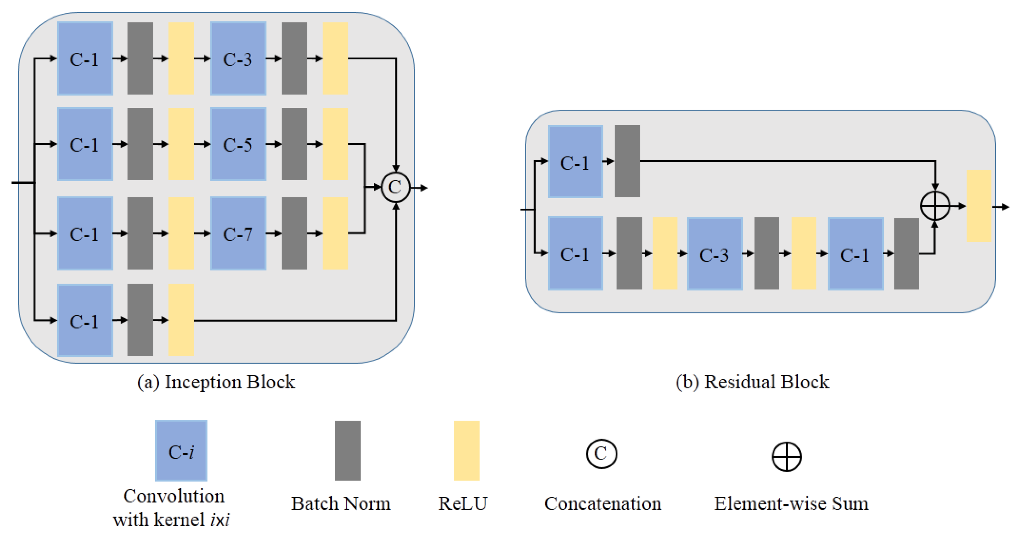
3.3. Inception and Residual Learning

The inception block is introduced to replace the convolutional layers (e.g., layers C, D, and F in Figure 3). The structure of the inception block is shown in Figure 5a, and the corresponding configurations are listed in Table 2. The inception block is composed of four branches. Three branches comprise two banks of convolution filters: the convolution size of the first is 1 × 1 , and the second is 3 × 3 , 5 × 5 , and 7 × 7 . The last branch comprises one bank of convolution filters with size 1 × 1 . Each convolution is followed by batch normalization and a rectified linear unit (ReLu). Convolution filters of different sizes are assembled in one inception block to enable multi-scale inference through the network.
The residual block in ERN is shown in Figure 5b, and the corresponding configurations are listed in Table 3. The residual block is composed of two branches. Branch one is a bank of convolution filters with size 1 × 1 , followed by batch normalization. Another branch consists of three banks of convolution filters with size 1 × 1 , 3 × 3 , and 1 × 1 . We use batch normalization after every convolution. An element-wise summation of two branches is carried out before the ReLu of the final convolution.

3.4. Joint Semantic Loss and Edge Loss

We denote the input training data set with N samples S = { ( X n , Y n , Y E n ) } n = 1 N , where X n = { x j ( n ) , j = 1 , , T } denotes the raw input image with T pixels. Y n = { y j ( n ) , j = 1 , , T } and Y E n = { y e j ( n ) , j = 1 , , T } denote the corresponding semantic ground truth and edge ground truth, respectively, for image X n . y j ( n ) = c denotes that the pixel belongs to the c t h semantic label where c { 1 , , C } . y e j ( n ) { 1 , 0 } denotes whether or not the pixel lies on an edge. It is worth mentioning that the edge ground truth is obtained by calculating the gradient of the semantic ground truth, Y E n = Y n .
For simplicity, we represent the collection of all standard network layer parameters by W . The semantic segmentation output and each edge output are associated with a classifier, in which the corresponding weights are denoted w s , w e n c o d e , and w d e c o d e .
The cross-entropy loss function summed over all pixels is used. However, when applied to semantic segmentation of remote sensing images [55] and edge detection tasks [29,56], the ordinary cross-entropy loss can be heavily affected by the imbalance of the class distribution. We adopted a weighted loss function where the calculation of trade-off weight for biased sampling is based on median frequency balancing [16].
The semantic loss is defined as:
L s e m a n t i c ( W , w s ) = j , n , c β c ( s e m a n t i c ) · log P r ( y j n = c | X ; W , w s ) ,
where β c ( s e m a n t i c ) = f r e q u e n c y ( c ) c f r e q u e n c y ( c ) denotes the weight of class c. P r denotes probability.
The encoder edge loss is defined as:
L e n e d g e ( W , w e n c o d e ) = β ( e d g e ) · j , n log P r ( y e j n = 1 | X ; W , w e n c o d e ) ( 1 β ( e d g e ) ) · j , n log P r ( y e j n = 0 | X ; W , w e n c o d e ) ,
where β ( e d g e ) = f r e q u e n c y ( e d g e ) f r e q u e n c y ( e d g e ) + f r e q u e n c y ( n o n e d g e ) indicates the weight of edge pixels and ( 1 β ( e d g e ) ) denotes the weight of non-edge pixels. The decoder edge loss L d e e d g e is identical to the encoder edge loss.
Putting the semantic loss and edge loss together, we minimize the following objective function via back-propagation:
( W , w ) * = a r g m i n ( α 1 · L s e m a n t i c ( W , w s ) + α 2 · L e n e d g e ( W , w e n c o d e ) + α 3 · L d e e d g e ( W , w d e c o d e ) ) ,
where α 1 , α 2 , and α 3 are continuous hyper-parameters and denote the weights of semantic loss, encoder edge loss, and decoder edge loss, respectively. In our experiments, the α 1 was fixed to 1, α 2 = α 3 = 20 for the UAV Image Dataset, and α 2 = α 3 = 4 for the ISPRS Vaihingen Dataset. More discussions about the value of α 1 , α 2 , and α 3 can be found in Section 5.1.

4. Experimental Design and Results

We performed extensive experiments to evaluate the effectiveness of the proposed ERN architecture. In this section, we describe the datasets used and our experimental settings, and report quantitative and qualitative results. The full implementation and trained networks are publicly available at: https://github.com/liushuo2018/ERN.

4.1. Datasets

We evaluated the proposed ERN on two datasets for semantic segmentation.
UAV Image Dataset. This dataset consists of 200 images which were obtained by a medium-altitude UAV in a plain region located in east China, where the main landforms include cities, villages, and open fields. The images were acquired by a visible light camera and composed of three channels: red (R), green (G) and blue (B). Each of the images has 1280 × 1024 pixels at a GSD (Ground Sample Distance) ranges from 35 cm to 60 cm. All of the image pixels were labeled as one of the following six classes: building, road, grassland, tree, land, and clutter. Half of the UAV images were randomly selected as the training sets, and the others were reserved for testing. Further information of this dataset will be updated in the project page.
ISPRS Vaihingen Dataset [35]. This dataset is publicly avaliable and consists of 33 very high resolution true orthophoto (TOP) tiles, as well as corresponding DSM (digital surface model) and nDSM (normalized digital surface model) data. TOP images were acquired by an airbone color-infrared camera and composed of three channels: near-infrared (NIR), red (R) and green (G). In addition, the corresponding DSM data was acquired by LiDAR and composed of one channel. Each of the tiles have ≈ 2500 × 2000 pixels at a GSD ≈ 9 cm. Pixels were labeled as one of the following six classes: impervious surfaces, building, low vegetation, tree, car, and clutter/background. Following the HSNet [24], eleven tiles (areas 1, 3, 5, 7, 13, 17, 21, 23, 26, 32, 37) were selected for training, while the other five tiles (areas: 11, 15, 28, 30, 34) were reserved for testing.

4.2. Training and Testing

Training. In the training phase, data augmentation was employed to mitigate overfitting. The images were split into fixed size patches ( 256 × 256 ) with 50% overlap. Each image patch was rotated at a 90 degree interval and flipped vertically and horizontally to produce eight augmented patches.
The adaptive moment estimation (ADAM) [57] optimization algorithm was used to train the networks. ADAM is a variant of stochastic gradient descent (SGD) with two moments m t = β 2 v t 1 + ( 1 β 2 ) g t 2 and v t = β 1 m t 1 + ( 1 β 1 ) g t ( g t is the pre-set first momentum). The update rule in ADAM is:
θ t + 1 = θ t η v t ^ + ϵ m t ^ ,
where m t ^ = m t 1 β 1 and v t ^ = v t 1 β 2 are the bias-corrected moments, and η is the learning rate. ( β 1 , β 2 , ϵ ) are parameters. In this paper, we chose β 1 = 0.9 , β 2 = 0.999 , ϵ = 10 8 . The learning rate was set to be divided by a factor of 10 every 10 epochs from an initial value of 10 5 . All the trainable parameters in the kernel of convolution and deconvolution layers were initialised following [58].
The training processes were performed on a Linux PC machine equipped with an single Nvidia GeForce 1080Ti graphics card. We implemented our deep network under Caffe [59] framework, and pre-processed original images with Python.
Testing. Limited by the GPU memory, the test images were also first split into small-size patches ( 256 × 256 ) to perform network inference. Then, the semantic segmentation result of the whole image was obtained by stitching the corresponding patch results. Overlap inference (OI) is widely used to mitigate erroneous artifacts caused by split and stitching pattern. We also performed multi-hypothesis prediction where the class for each pixel was identified in several overlapping patches to further improve the segmentation performance of whole image. In our overlap inference experiments, we classified overlapping patches with a stride of 128 pixels and then summed the results.
The testing processes were performed under the same environment with the training processes. In addition, the post-processing (stitching, multi-hypothesis prediction, etc) was also implemented with Python.

4.3. Evaluation Metrics

We used the same evaluation metrics as in HSNet [24] and evaluated the performance of different methods based on three criteria: per-class F-score, overall accuracy, and average F-score. The F-score is defined as:
F-score = 2 × p r e c i s i o n × r e c a l l ( p r e c i s i o n + r e c a l l ) .
The overall accuracy is the total number of correctly-labeled pixels divided by the total number of pixels.
In the UAV Image Dataset and ISPRS Vaihingen Dataset [35], the clutter class accounts for an extremely small number of pixels. As a result, we neglected the clutter class when reporting the results, following the common practice [23,24].

4.4. Results

We compare our results with those of FCN [17], SegNet [19], and HSNet [24]. To produce the results of the above baselines, we employed the publicly available networks provided by the original authors and trained them under the same settings in Section 4.2.

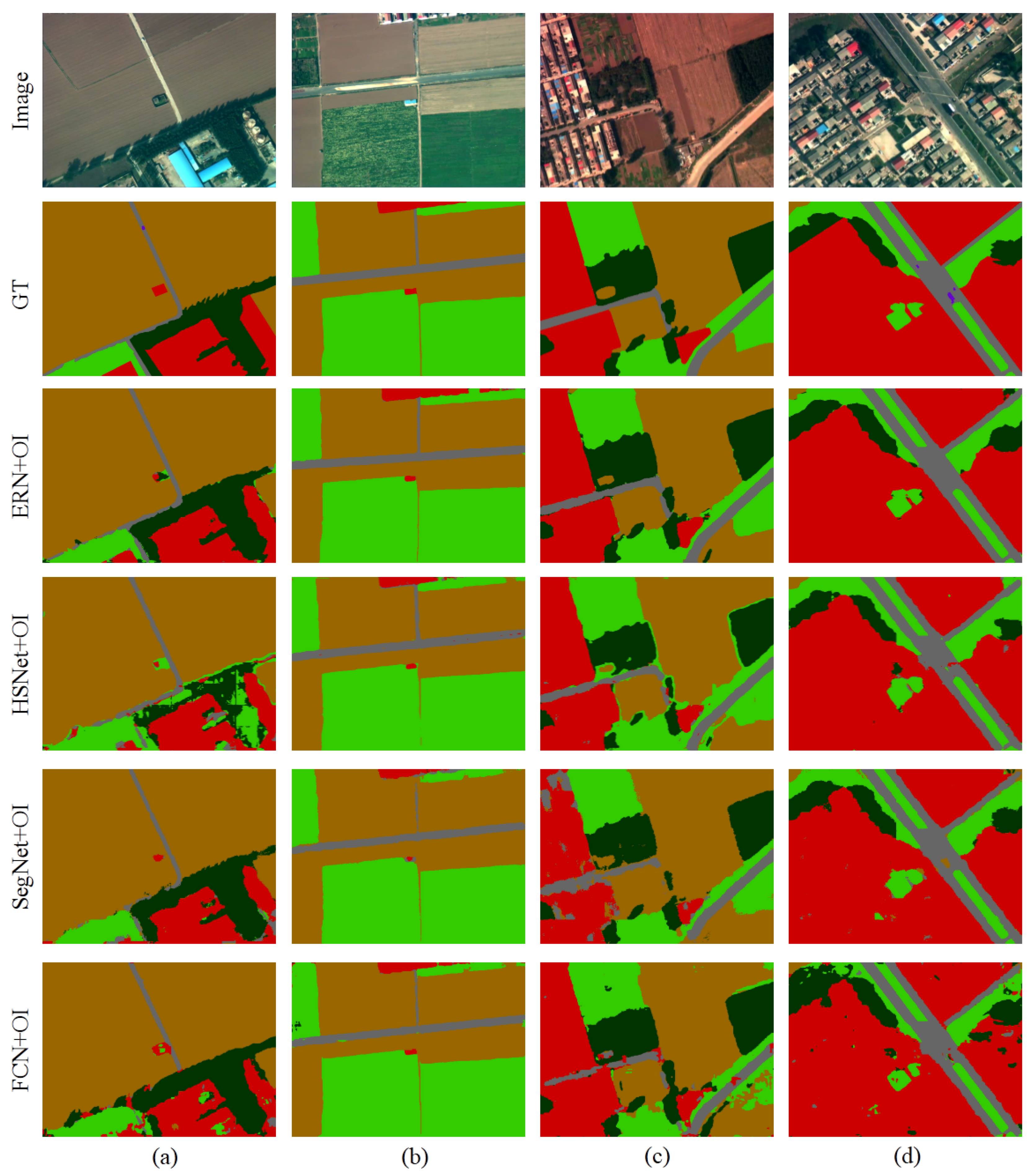
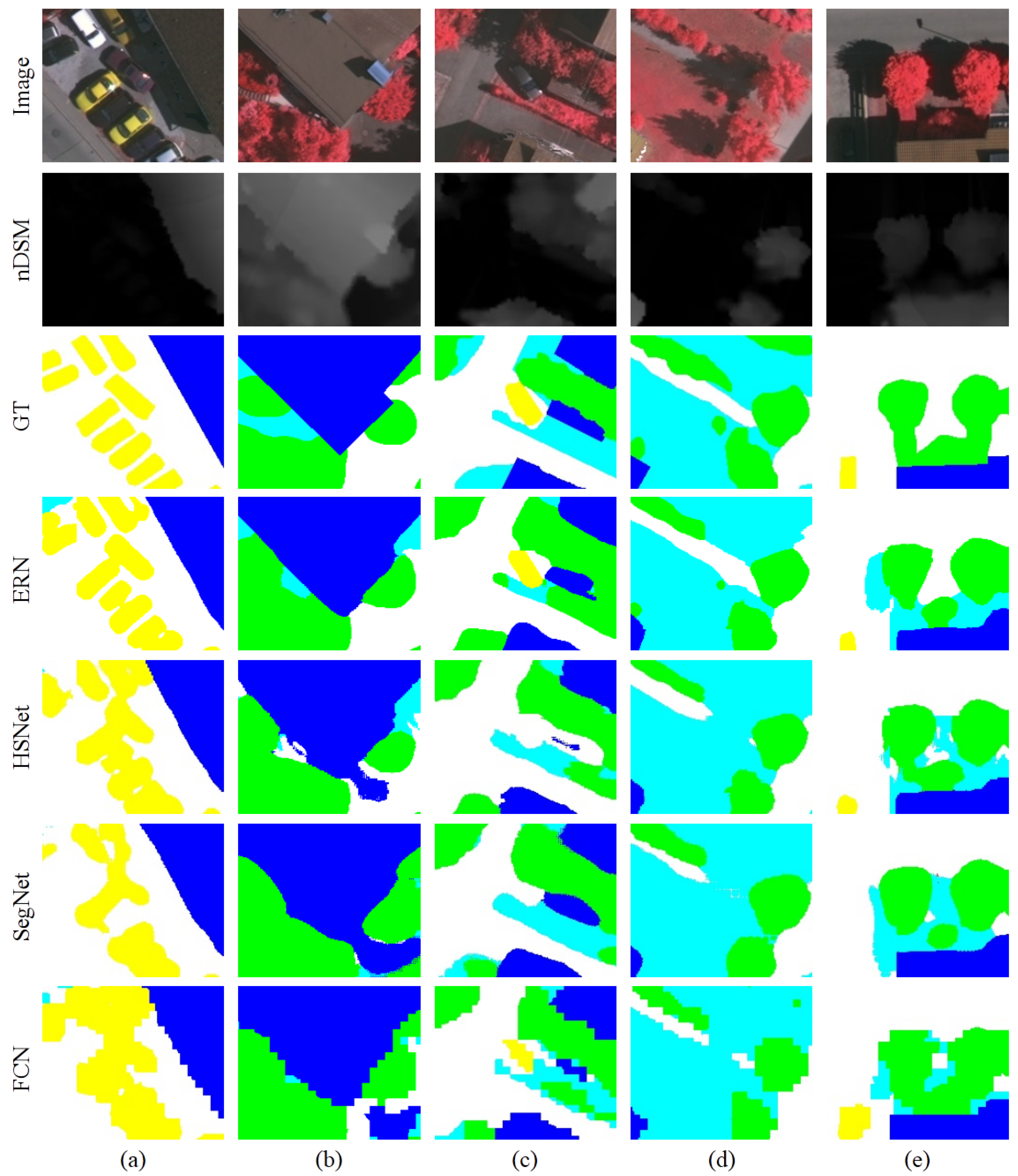
4.4.1. Results of UAV Image Dataset

Numerical results. Table 4 reports the experimental results obtained from the UAV images. The results are organized into two groups, corresponding to the normal inference results and overlap inference results. From the table, it can be observed that the proposed ERN outperformed the other networks. The average F-score and the overall accuracy of ERN reached 87.74% and 91.90%, respectively, and ERN showed a better performance for all classes. Overlap inference (OI) systematically improved the prediction accuracy for all methods and all classes. The average F-score and overall accuracy of ERN further increased to 88.81% and 92.66%, respectively. This proves the effectiveness of overlap inference. The confusion matrices are further provided in Appendix ATable A1.
Qualitative Results. For a visual demonstration, Figure 6 shows the semantic segmentation results for four complete UAV images, while Figure 7 magnifies certain areas, showing more detail.
From Figure 6, it can be observed that most of the methods performed well for buildings and land. The performance on the road, tree, and grass was relatively poor, especially at the boundaries between different regions. ERN had much cleaner boundary results than other methods. These results were consistent with the numerical results in Table 4.
Figure 7 presents some local results in detail, which better shows the strength of ERN. From Figure 7a, it can be seen that the shadows from trees posed great difficulties for semantic segmentation. Both FCN and SegNet labeled part of the road as a tree. HSNet managed to detect the road, but the segmentation accuracy was quite low. ERN successfully recognized the road, tree, grass, and land, even under shadows. In Figure 7b–e, the results of ERN outperformed the other models, giving much more accurate boundaries. We argue that the edge loss reinforced structures contributed to the good performance by improving the boundary accuracy and reducing semantic ambiguity between different regions.

4.4.2. Results of ISPRS Vaihingen Dataset

Numerical results. Aside from the conventional pixel-wise ground truth, border-eroded ground-truth label images are also available for the ISPRS Vaihingen Dataset. In these images, borders between classes are eroded with a disk radius of three pixels. We report results for both ground-truth versions. All pixels were considered for the conventional pixel-wise ground-truth version, while for the eroded version, border pixels were not accounted for.
Table 5 reports the results of different methods for the ISPRS Vaihingen Dataset. The F-scores for each class and overall performance are shown respectively for GT and er-GT (eroded ground-truth version). From the table, it can be observed that the proposed ERN outperformed the other networks. The average F-score and the overall accuracy of ERN reached 88.64% and 88.88%, respectively, and ERN reached a better performance for all classes. ERN improved the segmentation accuracy particularly well for the car class. It is worth mentioning that the experiments in Table 5 did not utilize overlap inference. The confusion matrices are further provided in Appendix ATable A2.
Qualitative Results. As a visual demonstration, Figure 8 shows the semantic segmentation results for the ISPRS Vaihingen Dataset, while Figure 9 shows certain areas in more detail. The ISPRS Vaihingen dataset provides a nDSM, which can help the network to distinguish buildings and surfaces, trees and vegetation. We connected the nDSM with near-infrared (NIR), red (R), and green (G) as an additional channel for all methods.
Figure 9 gives more results in detail. From Figure 9a, it can be seen that cars are very close to each other, and it is difficult to separate them with HSNet [24], SegNet [19], and FCN [17]. By introducing the edge loss reinforced structures, the proposed ERN can better separate densely located cars. Figure 9b shows that similar appearance between buildings and impervious surfaces confuses the network, but ERN correctly segmented neighboring regions. Moreover, Figure 9c–e show that the shadows from trees or buildings pose difficulties for semantic segmentation. In this case, ERN segmented the impervious surfaces and low vegetation with a higher accuracy. We argue that the edge loss reinforced structures helped improve the boundary accuracy in regions without effective infromation from the nDSM.

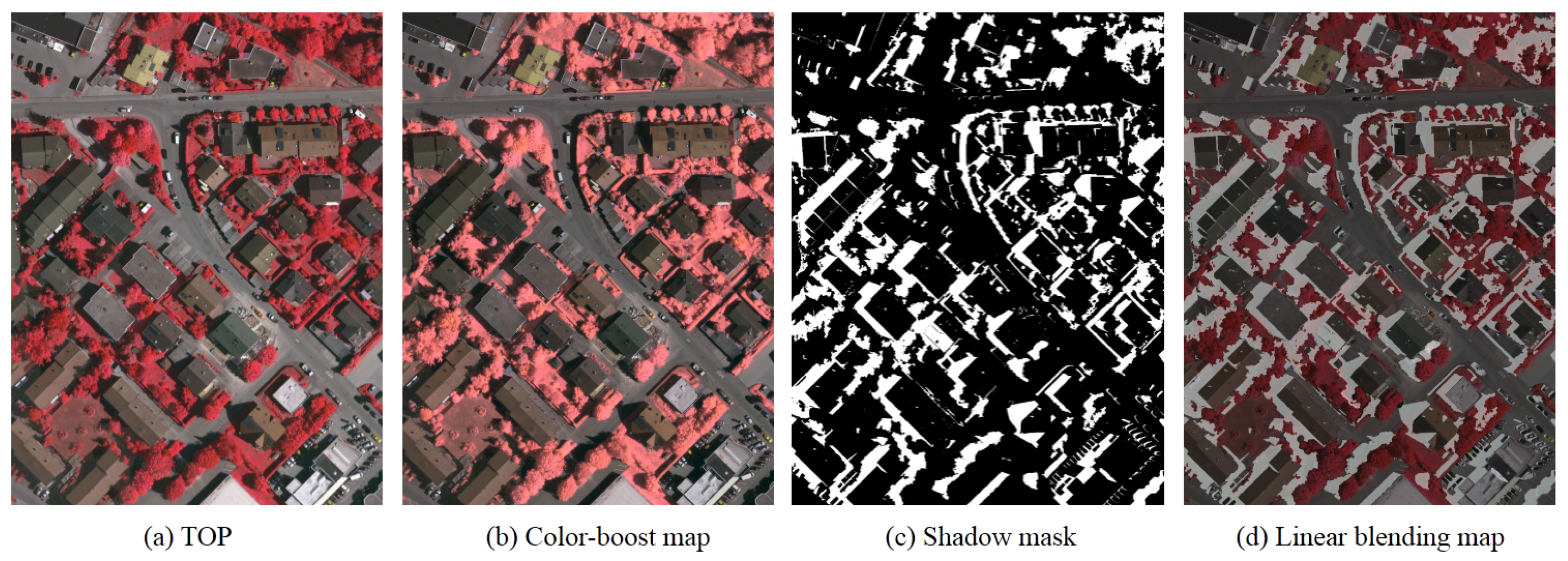
4.5. Performance in Shadow-Affected Regions

In this section, we present the performance of semantic segmentation in shadow-affected regions. The major challenge for comparison comes from the fact that there is no ground truth to indicate which pixel is covered by shadow. Traditional unsupervised shadow detection methods [60] often failed in the dark regions, such as black cars and roofs. Therefore, we manually labeled the shadow masks for the test tiles (areas: 11, 15, 28, 30, 34) in ISPRS Vaihingen Dataset [35]. We first pre-processed the original images with the contrast preserving decolorization technology [61], which can help human better separate shadow regions from surroundings. And the semantic ground truth was also utilized to help distinguish whether the pixel belongs to the shadow or dark-color cars during annotation. Figure 10 shows an example of the labeled shadow mask. According to statistics, 15%∼25% of the pixels are in shadow. And the shadow-affected pixels are mainly located in the regions of impervious surfaces and low vegetation.
The semantic segmentation performance in the shadow-affected regions has been re-evaluated and listed in Table 6. Compared with the results in whole image (see Table 5), the performance in shadow-affected regions is much poorer due to the interference of shadow. From Table 6, it can be observed that the proposed ERN outperforms the other networks. ERN reaches the best performance in F-scores of all classes, average F-score and the overall accuracy, which demonstrates its effectiveness and robustness in shadow-affected regions.

5. Discussion

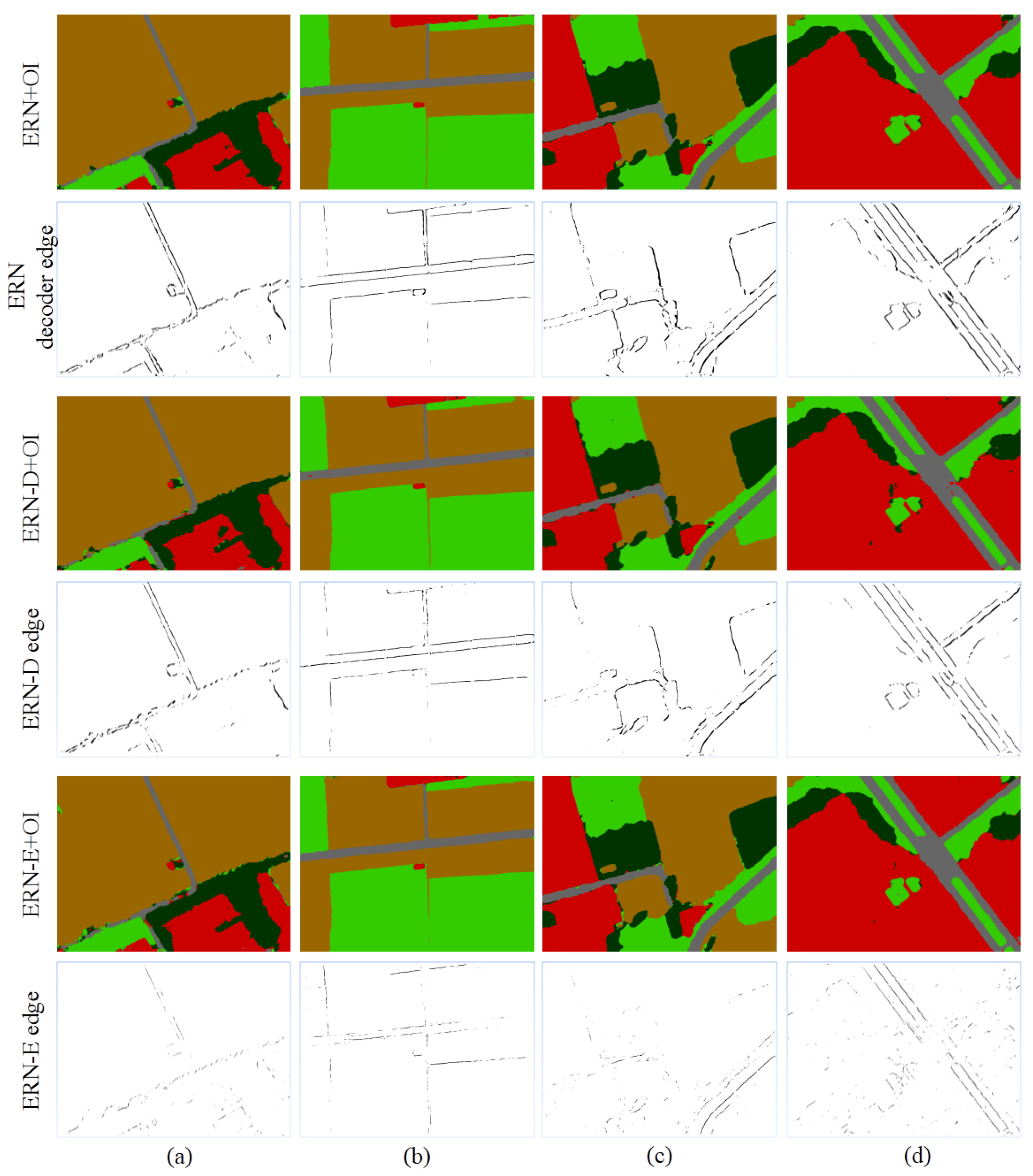
5.1. Edge Loss Analysis

To evaluate the performance brought by edge loss reinforced structures in the proposed ERN, extensive experiments of different edge loss constraints were further conducted. ERN includes two edge loss reinforced structures: encoder edge and decoder edge. In this section, we explore two variations of ERN—ERN-E and ERN-D, which are shown in Figure 11. ERN-E is the encoder–decoder semantic segmentation net with only the encoder edge, while ERN-D uses only the decoder edge. The training process for ERN-E and ERN-D is identical to ERN.
Table 7 reports the experimental results on the UAV images for ERN, ERN-E, and ERN-D with different edge loss weight. The edge loss weight in ERN-E and ERN-D are denoted as α e n and α d e , respectively. Figure 12 shows the comparison of semantic output predictions and edge output predictions of ERN, ERN-E, and ERN-D.
When setting α e n = α d e 1 , the performance of ERN-E and ERN-D was slightly decreased compared with the original encoder–decoder framework. We checked the edge structure and found that it output hardly any edge information. When setting α e n = α d e = 10 , the performances of ERN-E and ERN-D were improved. We found that the edge structure could correctly output the edge information; see Figure 12. Under the same edge loss weight, ERN ( α 1 = 1 , α 2 = α 3 = 10 ) clearly outperformed the ERN-E ( α e n = 10 ) and ERN-D ( α d e = 10 ); see Table 7 and Figure 12. Comparing the edge results of ERN and ERN-D from Figure 12, we found that the edge predictions from the ERN (decoder edge) were superior to those from ERN-D.
We argue that the edge loss reinforced structure can be incorporated into any encoder–decoder architecture with a simple modification. The instructions are as follows: (1) the edge loss weight ( α e d g e ) should be larger than the semantic loss weight ( α s e m a n t i c ), because the edge loss ( L e d g e ) is always smaller than the semantic loss ( L s e m a n t i c ). A too-small edge loss weight may lead to a failure of edge supervision; (2) the edge loss weight may differ between datasets, which helps the different kinds of losses ( α s e m a n t i c · L s e m a n t i c , α e d g e · L e d g e ) adapt to the same order of magnitude; and (3) the performance gain of semantic prediction is proportional to the accuracy of edge prediction, indicating that a better edge detection improves semantic segmentation.

5.2. General Analysis

To the best of our knowledge, the most similar works to our ERN are from Chen et al. [32] and Cheng et al. [33], where they build edge-aware nets to further filter the semantic segmentation results using domain transfer technology and regularization method, respectively. ERN constructs multiple edge loss reinforced structures from the encoder and decoder separately (namely, encoder edge and decoder edge), while only one edge-aware net has been constructed in [32] (similar to our encoder edge) and [33] (constructed by concatenating hierarchical features cross encoder and decoder). Multiple structures and corresponding weighted edge losses are introduced to strengthen the ability of preserving the boundary information rather than post-fine-tuning the semantic segmentation results. The encoder edge loss leverages the benefits of deep supervision in shallow layers like HED [29], and the decoder one aims to further assist the high-level semantic parsing. Moreover, the weighted style of edge loss helps better shape and reinforce the semantic segmentation net.
Compared with the models for general images, the network designed for remote sensing images should not only face the inherent difficulties of semantic segmentation, but also deal with the special issues derived from characters of remote sensing images. Thus, this paper mainly focuses on improving the poor segmentation performance caused by appearance similarity and shadow interference, which are ubiquitous in remote sensing images.
The experimental results in Section 4 demonstrate that our approach achieves state-of-the-art performance on two remote sensing datasets. The proposed approach outperforms reference methods by substantial margins in terms of both average F-score and overall accuracy. In particular, the easily confusing pixels with similar visual appearance have been correctly labeled (See Figure 9b,c). In addition, the semantic segmentation performance is also significantly improved in the challenging situation of shadow interference (See Figure 7a and Figure 9d,e). Specifically, the shadow masks have been manually labeled and the numerical comparison within the shadow-affected regions has been further reported in Section 4.5, which shows the advantage of the proposed ERN.
We attribute the effectiveness of the proposed approach mainly to the design of multiple weighted edge loss reinforced structures in the network. The above two problems are essentially due to the low inter-class variance and the large semantic ambiguity, which make it difficult for the network to correctly distinguish different semantics. By introducing the multiple weighted edge loss reinforced structures, more boundary information can be preserved in the network and further helps to reduce the semantic ambiguity.
It is interesting to find that our approach significantly improves the segmentation accuracy of car in the ISPRS Vaihingen dataset. The low accuracy of car segmentation is usually thought to be caused by the small sample number. However, we find that the surface between cars is often incorrectly classified when the cars are extremely close to each other (see Figure 9a). We argue that the boundary information help the network better segment cars.

5.3. Efficiency Limitation

Even though ERN provides the best overall accuracy and average F-score, it requires the highest segmentation time when compared with other networks. The efficiency of ERN is one of the biggest limitations.
Table 8 shows the average semantic segmentation time per image on the test dataset (100 images for UAV Image Dataset, five images for ISPRS Vaihingen Dataset). The running time list in the Table 8 is the sum of inference time and stitching time. The proposed ERN takes 118.83 s and 19.55 s to finish inference and stitching on the test images of UAV Image Dateset and ISPRS Vaihingen Dataset respectively. The environment is same as Section 4.2.

5.4. Future Work

Possible directions for future research include designing a more powerful edge loss reinforced structure while keeping efficiency for high quality semantic segmentation and automatically learning the edge loss weight rather than based on empirical settings.

6. Conclusions

Semantic segmentation for remote sensing images is a challenging task due to low inter-class variance and interference from areas containing shadows. In this paper, we present a new end-to-end semantic segmentation network. By introducing multiple weighted edge loss reinforced structures, the spatial boundary information is preserved and used to reduce semantic ambiguity. The performance of semantic segmentation is significantly improved in the whole image as well as the shadow-affected regions. On the UAV Image Dataset and ISPRS Vaihingen Dataset [35], the average F-score of ERN has reached 88.81% and 88.64%, and the overall accuracy has reached 92.66% and 88.88%, respectively. In addition, the F-score of Car has been impressively improved nearly 7%. In addition, the edge loss reinforced structures share most network parameters with the original network, indicating that additional structure does not greatly increase model complexity. Finally, we have compared and analyzed different edge loss constraints and clarified the working conditions where edge detection promotes semantic segmentation. The edge loss reinforced structure can be easily integrated into any encoder–decoder semantic segmentation networks. The full implementation in this project is available at: https://github.com/liushuo2018/ERN.

Author Contributions

Conceptualization, S.L. and Y.L.; Data curation, Y.W.; Funding acquisition, W.D. and H.L.; Investigation, S.L. and C.L.; Methodology, S.L., W.D. and Y.L.; Project administration, C.L.; Resources, W.D.; Software, S.L. and Y.L.; Supervision, W.D.; Validation, S.L. and C.L.; Visualization, C.L.; Writing—Original draft, S.L., Y.L. and Y.W.; Writing—Review and editing, W.D. and H.L.

Acknowledgments

This work was supported by the National Key Research and Development Program of China (Grant No. 2016YFB0502600) and the National Natural Science Foundation of China (Grant No. 61601014).

Conflicts of Interest

The authors declare no conflict of interest.

Appendix A. Confusion Matrices

In this section, we report the confusion matrices for both the proposed ERN and the reference techniques tested on the UAV Image Dateset and ISPRS Vaihingen Dataset. The values are given in percentages, and the diagonal elements are highlighted in bold.
Table A1. Confusion matrix on the UAV Image Dateset.
BuildingsRoadGrassTreeLand
FCN [17]Buildings89.901.471.916.100.62
Road7.583.163.51.93.94
Grass2.440.6374.1019.533.3
Tree8.280.261.5287.902.04
Land1.090.382.662.8193.06
SegNet [19]Buildings86.494.642.342.863.67
Road2.0478.672.200.6616.42
LowVeg0.820.8781.0413.413.87
Tree7.520.452.6579.889.5
Land0.150.182.160.4997.03
HSNet [24]Buildings91.281.973.333.160.26
Road8.0384.215.320.252.18
Grass2.120.7792.463.291.37
Tree10.901.026.7978.442.58
Land0.390.685.460.2993.18
ERNBuildings92.941.121.114.490.33
Road9.5784.252.601.352.23
Grass0.940.7290.286.441.62
Tree6.770.597.0982.343.21
Land0.220.373.260.9295.22
Table A2. Confusion matrix on the ISPRS Vaihingen Dataset. Imp.Surf: impervious surface; LowVeg: low vegetation.
Imp.SurfBuildingsLowVegTreeCar
FCN [17]Imp.Surf88.993.145.391.091.38
Buildings3.8993.212.220.570.11
LowVeg5.882.4774.1117.320.22
Tree0.920.379.3689.350.01
Car15.601.711.000.5781.11
SegNet [19]Imp.Surf91.682.463.871.180.81
Buildings4.1693.222.020.550.05
LowVeg6.622.4473.6317.220.09
Tree0.930.4614.2884.320.01
Car17.310.800.900.7280.27
HSNet [24]Imp.Surf92.642.543.710.650.46
Buildings3.5094.112.180.180.03
LowVeg6.732.4478.0912.670.08
Tree1.240.3510.9687.440.01
Car15.911.961.220.3280.59
ERNImp.Surf91.182.634.621.130.33
Buildings2.6794.802.150.350.02
LowVeg5.071.8877.9615.060.03
Tree0.800.208.8290.170.01
Car6.393.070.460.7189.23

References

  1. Plaza, A.; Plaza, J.; Paz, A.; Sanchez, S. Parallel Hyperspectral Image and Signal Processing [Applications Corner]. IEEE Signal Process. Mag. 2011, 28, 119–126. [Google Scholar] [CrossRef]
  2. Cheng, G.; Han, J.; Lu, X. Remote Sensing Image Scene Classification: Benchmark and State of the Art. Proc. IEEE 2017, 105, 1865–1883. [Google Scholar] [CrossRef] [Green Version]
  3. Zhang, B.; Gu, J.; Chen, C.; Han, J.; Su, X.; Cao, X.; Liu, J. One-two-one networks for compression artifacts reduction in remote sensing. ISPRS J. Photogramm. Remote Sens. 2018. [Google Scholar] [CrossRef]
  4. Zhu, X.X.; Tuia, D.; Mou, L.; Xia, G.; Zhang, L.; Xu, F.; Fraundorfer, F. Deep Learning in Remote Sensing: A Comprehensive Review and List of Resources. IEEE Geosci. Remote Sens. Mag. 2017, 5, 8–36. [Google Scholar] [CrossRef] [Green Version]
  5. Farabet, C.; Couprie, C.; Najman, L.; LeCun, Y. Learning hierarchical features for scene labeling. IEEE Trans. Pattern Anal. Mach. Intell. 2013, 35, 1915–1929. [Google Scholar] [CrossRef] [PubMed] [Green Version]
  6. Gaetano, R.; Scarpa, G.; Poggi, G. Hierarchical Texture-Based Segmentation of Multiresolution Remote-Sensing Images. IEEE Trans. Geosci. Remote Sens. 2009, 47, 2129–2141. [Google Scholar] [CrossRef]
  7. Martha, T.R.; Kerle, N.; Van Westen, C.J.; Jetten, V.G.; Kumar, K.V. Segment Optimization and Data-Driven Thresholding for Knowledge-Based Landslide Detection by Object-Based Image Analysis. IEEE Trans. Geosci. Remote Sens. 2011, 49, 4928–4943. [Google Scholar] [CrossRef]
  8. Yao, X.; Han, J.; Cheng, G.; Qian, X.; Guo, L. Semantic Annotation of High-Resolution Satellite Images via Weakly Supervised Learning. IEEE Trans. Geosci. Remote Sens. 2016, 54, 3660–3671. [Google Scholar] [CrossRef]
  9. Liu, Y.; Fan, B.; Wang, L.; Bai, J.; Xiang, S.; Pan, C. Semantic labeling in very high resolution images via a self-cascaded convolutional neural network. ISPRS J. Photogramm. Remote Sens. 2017. [Google Scholar] [CrossRef]
  10. Marcos, D.; Volpi, M.; Kellenberger, B.; Tuia, D. Land cover mapping at very high resolution with rotation equivariant CNNs: Towards small yet accurate models. ISPRS J. Photogramm. Remote Sens. 2018. [Google Scholar] [CrossRef]
  11. Blaschke, T. Object based image analysis for remote sensing. ISPRS J. Photogramm. Remote Sens. 2010, 65, 2–16. [Google Scholar] [CrossRef]
  12. Wang, P.; Huang, C.; Tilton, J.C.; Tan, B.; Colstoun, E.C.B.D. HOTEX: An approach for global mapping of human built-up and settlement extent. In Proceedings of the IEEE International Geoscience and Remote Sensing Symposium, Fort Worth, TX, USA, 23–28 July 2017. [Google Scholar]
  13. Liu, T.; Abd-Elrahman, A.; Zare, A.; Dewitt, B.A.; Flory, L.; Smith, S.E. A fully learnable context-driven object-based model for mapping land cover using multi-view data from unmanned aircraft systems. Remote Sens. Environ. 2018, 216, 328–344. [Google Scholar] [CrossRef]
  14. Chen, G.; Weng, Q.; Hay, G.J.; He, Y. Geographic object-based image analysis (GEOBIA): Emerging trends and future opportunities. GISci. Remote Sens. 2018, 55, 159–182. [Google Scholar] [CrossRef]
  15. Mostajabi, M.; Yadollahpour, P.; Shakhnarovich, G. Feedforward semantic segmentation with zoom-out features. In Proceedings of the IEEE Conference on Computer Vision and Pattern Recognition, Boston, MA, USA, 7–12 June 2015; pp. 3376–3385. [Google Scholar]
  16. Eigen, D.; Fergus, R. Predicting Depth, Surface Normals and Semantic Labels with a Common Multi-scale Convolutional Architecture. In Proceedings of the IEEE International Conference on Computer Vision, Washington, DC, USA, 7–13 December 2016. [Google Scholar]
  17. Long, J.; Shelhamer, E.; Darrell, T. Fully convolutional networks for semantic segmentation. In Proceedings of the IEEE Conference on Computer Vision and Pattern Recognition, Boston, MA, USA, 7–12 June 2015; pp. 3431–3440. [Google Scholar]
  18. Noh, H.; Hong, S.; Han, B. Learning Deconvolution Network for Semantic Segmentation. In Proceedings of the IEEE Conference on Computer Vision and Pattern Recognition, Boston, MA, USA, 7–12 June 2015. [Google Scholar]
  19. Badrinarayanan, V.; Kendall, A.; Cipolla, R. SegNet: A Deep Convolutional Encoder-Decoder Architecture for Scene Segmentation. IEEE Transact. Pattern Anal. Machine Intell. 2017, 39, 2481–2495. [Google Scholar] [CrossRef] [PubMed]
  20. Lin, G.; Milan, A.; Shen, C.; Reid, I.D. RefineNet: Multi-path Refinement Networks for High-Resolution Semantic Segmentation. IEEE Conf. Comput. Vis. Pattern Recognit. 2017, 1, 5168–5177. [Google Scholar]
  21. Zhao, H.; Shi, J.; Qi, X.; Wang, X.; Jia, J. Pyramid Scene Parsing Network. In Proceedings of the IEEE Conference on Computer Vision and Pattern Recognition (CVPR), Honolulu, HI, USA, 21–26 July 2017; pp. 2881–2890. [Google Scholar]
  22. Ronneberger, O.; Fischer, P.; Brox, T. U-Net: Convolutional Networks for Biomedical Image Segmentation. In Proceedings of the International Conference on Medical Image Computing and Computer Assisted Intervention, Quebec, QC, Canada, 10–14 September 2015. [Google Scholar]
  23. Volpi, M.; Tuia, D. Dense Semantic Labeling of Subdecimeter Resolution Images With Convolutional Neural Networks. IEEE Trans. Geosci. Remote Sens. 2017, 55, 881–893. [Google Scholar] [CrossRef] [Green Version]
  24. Liu, Y.; Minh Nguyen, D.; Deligiannis, N.; Ding, W.; Munteanu, A. Hourglass-ShapeNetwork Based Semantic Segmentation for High Resolution Aerial Imagery. Remote Sens. 2017, 9, 522. [Google Scholar] [CrossRef]
  25. Ghiasi, G.; Fowlkes, C.C. Laplacian Pyramid Reconstruction and Refinement for Semantic Segmentation. In Proceedings of the European Conference on Computer Vision, Amsterdam, The Netherlands, 8–16 October 2016. [Google Scholar]
  26. Kohli, P.; Torr, P.H.S. Robust higher order potentials for enforcing label consistency. Int. J. Comput. Vis. 2009, 82, 302–324. [Google Scholar] [CrossRef]
  27. Russell, C. Associative hierarchical CRFs for object class image segmentation. In Proceedings of the IEEE International Conference on Computer Vision, Angers, France, 17–21 May 2010. [Google Scholar]
  28. Arnab, A.; Jayasumana, S.; Zheng, S.; Torr, P.H.S. Higher Order Conditional Random Fields in Deep Neural Networks. In Proceedings of the European Conference on Computer Vision, Amsterdam, The Netherlands, 8–16 October 2016. [Google Scholar]
  29. Xie, S.; Tu, Z. Holistically-nested edge detection. In Proceedings of the IEEE Conference on Computer Vision and Pattern Recognition, Boston, MA, USA, 7–12 June 2015; pp. 1395–1403. [Google Scholar]
  30. Bertasius, G.; Shi, J.; Torresani, L. High-for-Low and Low-for-High: Efficient Boundary Detection from Deep Object Features and Its Applications to High-Level Vision. In Proceedings of the IEEE International Conference on Computer Vision, Washington, DC, USA, 7–13 December 2015; pp. 504–512. [Google Scholar]
  31. Kokkinos, I. Pushing the Boundaries of Boundary Detection using Deep Learning. In Proceedings of the International Conference on Learning Representations, San Juan, PR, USA, 2–4 May 2016. [Google Scholar]
  32. Chen, L.C.; Barron, J.T.; Papandreou, G.; Murphy, K.; Yuille, A.L. Semantic Image Segmentation with Task-Specific Edge Detection Using CNNs and a Discriminatively Trained Domain Transform. In Proceedings of the IEEE Conference on Computer Vision and Pattern Recognition, Las Vegas, NV, USA, 27–30 June 2016; pp. 4545–4554. [Google Scholar]
  33. Cheng, D.; Meng, G.; Xiang, S.; Pan, C. FusionNet: Edge Aware Deep Convolutional Networks for Semantic Segmentation of Remote Sensing Harbor Images. IEEE J. Sel. Top. Appl. Earth Obs. Remote Sens. 2017, 10, 5769–5783. [Google Scholar] [CrossRef]
  34. Marmanis, D.; Schindler, K.; Wegner, J.D.; Galliani, S.; Datcu, M.; Stilla, U. Classification with an edge: Improving semantic image segmentation with boundary detection. ISPRS J. Photogramm. Remote Sens. 2018, 135, 158–172. [Google Scholar] [CrossRef] [Green Version]
  35. ISPRS 2D Semantic Labeling Contest. Available online: http://www2.isprs.org/commissions/comm3/ wg4/2d-sem-label-vaihingen.html (accessed on 7 July 2018).
  36. Garciagarcia, A.; Ortsescolano, S.; Oprea, S.; Villenamartinez, V.; Rodriguez, J.G. A Review on Deep Learning Techniques Applied to Semantic Segmentation. arXiv, 2017; arXiv:1704.06857. [Google Scholar]
  37. Simonyan, K.; Zisserman, A. Very Deep Convolutional Networks for Large-Scale Image Recognition. Available online: http://arxiv.org/pdf/1409.1556v6.pdf (accessed on 18 December 2015).
  38. Zhang, B.; Yang, Y.; Chen, C.; Yang, L.; Han, J.; Shao, L. Action Recognition Using 3D Histograms of Texture and A Multi-class Boosting Classifier. IEEE Trans. Image Process. 2017, 26, 4648–4660. [Google Scholar] [CrossRef] [PubMed]
  39. Luan, S.; Chen, c.; Zhang, B.; han, j.; Liu, J. Gabor Convolutional Networks. IEEE Trans. Image Process. 2018, 27, 4357–4366. [Google Scholar] [CrossRef] [PubMed] [Green Version]
  40. Comaniciu, D.; Meer, P. Mean shift: A robust approach toward feature space analysis. IEEE Trans. Pattern Anal. Mach. Intell. 2002, 24, 603–619. [Google Scholar] [CrossRef]
  41. Felzenszwalb, P.F.; Huttenlocher, D.P. Efficient Graph-Based Image Segmentation. Int. J. Comput. Vis. 2004, 59, 167–181. [Google Scholar] [CrossRef] [Green Version]
  42. Achanta, R.; Shaji, A.; Smith, K.; Lucchi, A.; Fua, P.; Susstrunk, S. SLIC Superpixels Compared to State-of-the-Art Superpixel Methods. IEEE Trans. Pattern Anal. Mach. Intell. 2012, 34, 2274–2282. [Google Scholar] [CrossRef] [PubMed] [Green Version]
  43. Shotton, J.; Johnson, M.; Cipolla, R. Semantic texton forests for image categorization and segmentation. In Proceedings of the IEEE Conference on Computer Vision and Pattern Recognition, Anchorage, AK, USA, 23–28 June 2008; pp. 1–8. [Google Scholar]
  44. He, K.; Zhang, X.; Ren, S.; Sun, J. Deep residual learning for image recognition. In Proceedings of the IEEE Conference on Computer Vision and Pattern Recognition, Las Vegas, NV, USA, 26 June–1 July 2016; pp. 770–778. [Google Scholar]
  45. Yu, F.; Koltun, V. Multi-Scale Context Aggregation by Dilated Convolutions. In Proceedings of the International Conference on Learning Representations, San Juan, PR, 2–4 May 2016. [Google Scholar]
  46. Chen, L.; Papandreou, G.; Kokkinos, I.; Murphy, K.P.; Yuille, A.L. Semantic Image Segmentation with Deep Convolutional Nets and Fully Connected CRFs. In Proceedings of the International Conference on Learning Representations, San Diego, CA, USA, 7–9 May 2015. [Google Scholar]
  47. Chen, L.; Papandreou, G.; Kokkinos, I.; Murphy, K.P.; Yuille, A.L. DeepLab: Semantic Image Segmentation with Deep Convolutional Nets, Atrous Convolution, and Fully Connected CRFs. IEEE Trans. Pattern Anal. Mach. Intell. 2018, 40, 834–848. [Google Scholar] [CrossRef] [PubMed] [Green Version]
  48. Persello, C.; Stein, A. Deep Fully Convolutional Networks for the Detection of Informal Settlements in VHR Images. IEEE Geosci. Remote Sens. Lett. 2017, 14, 2325–2329. [Google Scholar] [CrossRef]
  49. Zheng, S.; Jayasumana, S.; Romera-Paredes, B.; Vineet, V.; Su, Z.; Du, D.; Huang, C.; Torr, P.H.S. Conditional Random Fields as Recurrent Neural Networks. In Proceedings of the IEEE Conference on International Conference on Computer Vision, Los Alamitos, CA, USA, 7–13 December 2015. [Google Scholar]
  50. Maggiori, E.; Tarabalka, Y.; Charpiat, G.; Alliez, P. High-Resolution Aerial Image Labeling with Convolutional Neural Networks. IEEE Trans. Geosci. Remote Sens. 2017, 55, 7092–7103. [Google Scholar] [CrossRef]
  51. Lee, C.; Xie, S.; Gallagher, P.W.; Zhang, Z.; Tu, Z. Deeply-Supervised Nets. In Proceedings of the International Conference on Artificial Intelligence and Statistics, San Diego, CA, USA, 9–12 May 2015; pp. 562–570. [Google Scholar]
  52. Hou, Q.; Cheng, M.; Hu, X.; Borji, A.; Tu, Z.; Torr, P.H.S. Deeply Supervised Salient Object Detection with Short Connections. In Proceedings of the IEEE Conference on Computer Vision and Pattern Recognition, Honplulu, HI, USA, 21–26 July 2017; pp. 5300–5309. [Google Scholar]
  53. Ke, W.; Chen, J.; Jiao, J.; Zhao, G.; Ye, Q. SRN: Side-Output Residual Network for Object Symmetry Detection in the Wild. In Proceedings of the IEEE Conference on Computer Vision and Pattern Recognition, Honplulu, HI, USA, 21–26 July 2017; pp. 302–310. [Google Scholar]
  54. Szegedy, C.; Liu, W.; Jia, Y.; Sermanet, P.; Reed, S.E.; Anguelov, D.; Erhan, D.; Vanhoucke, V.; Rabinovich, A. Going deeper with convolutions. In Proceedings of the IEEE Conference on Computer Vision and Pattern Recognition, Boston, MA, USA, 7–12 June 2015; pp. 1–9. [Google Scholar]
  55. Kampffmeyer, M.; Salberg, A.B.; Jenssen, R. Semantic Segmentation of Small Objects and Modeling of Uncertainty in Urban Remote Sensing Images Using Deep Convolutional Neural Networks. In Proceedings of the IEEE Conference on Computer Vision and Pattern Recognition, Las Vegas, NV, USA, 26 June–1 July 2016. [Google Scholar]
  56. Hwang, J.J.; Liu, T.L. Pixel-wise Deep Learning for Contour Detection. arXiv, 2015; arXiv:1504.01989. [Google Scholar]
  57. Kingma, D.; Ba, J. Adam: A method for stochastic optimization. arXiv, 2014; arXiv:1412.6980. [Google Scholar]
  58. He, K.; Zhang, X.; Ren, S.; Sun, J. Delving Deep into Rectifiers: Surpassing Human-Level Performance on ImageNet Classification. In Proceedings of the IEEE International Conference on Computer Vision, Washington, DC, USA, 7–13 December 2016. [Google Scholar]
  59. Jia, Y.; Shelhamer, E.; Donahue, J.; Karayev, S.; Long, J.; Girshick, R.; Guadarrama, S.; Darrell, T. Caffe: Convolutional Architecture for Fast Feature Embedding. In Proceedings of the Acm International Conference on Multimedia, Orlando, FL, USA, 3–7 November 2014; pp. 675–678. [Google Scholar]
  60. Tsai, V.J.D. A comparative study on shadow compensation of color aerial images in invariant color models. IEEE Trans. Geosci. Remote Sens. 2006, 44, 1661–1671. [Google Scholar] [CrossRef]
  61. Lu, C.; Xu, L.; Jia, J. Contrast preserving decolorization. In Proceedings of the IEEE International Conference on Computational Photography, Seattle, WA, USA, 28–29 April 2012; pp. 1–7. [Google Scholar]
Figure 1. Examples of remote sensing images that are challenging for semantic segmentation. (a) similar appearance between a building and its surroundings, in which the impervious surface was incorrectly recognized as a building by HSNet [24], SegNet [19], and FCN [17]. white: impervious surface; blue: buildings; cyan: low vegetation; green: trees. (b) interference of shadows, which results in poor performance; red: buildings; gray: roads; bright green: grass; dark green: trees; brown: land.
Remotesensing 10 01339 g001
Figure 2. Framework of the proposed edge loss reinforced semantic segmentation network (ERN). The encoder edge and decoder edge are constructed to promote the semantic segmentation. In the training phase, the semantic ground truth (GT) and edge ground truth simultaneously provide the supervision information in different layers. Thus, the loss ( L ) of the network includes semantic loss ( L s e m a n t i c ) and edge loss ( L e n e d g e , L d e e d g e ).
Remotesensing 10 01339 g002
Figure 3. Architecture of the proposed ERN. A, B, H, I, and J are convolutional layers; C, D, and F are inception blocks; B-r and C-r are residual blocks; E, G, S, B-e, C-e, F-e, and H-e are deconvolutional layers.
Remotesensing 10 01339 g003
Figure 4. Illustration of different architectures. HED [29] and DSS [52] have several side output losses and one fuse loss. Our edge structure is much simpler.
Remotesensing 10 01339 g004
Figure 5. Structure of the inception block and the residual block.
Remotesensing 10 01339 g005
Figure 6. Semantic segmentation results of the UAV images from ERN, HSNet [24], SegNet [19] and FCN [17]. GT: ground truth. OI: overlap inference. (ad) are four different scenes of UAV images, ranging from villages to cities; red: buildings; gray: roads; bright green: grass; dark green: trees; brown: land; purple: clutter.
Remotesensing 10 01339 g006
Figure 7. Semantic segmentation results for some local details of the UAV images. (a) shadow-affected region; (b) similar appearance between road and land; (ce) challenge cases near the boundary; red: buildings; gray: roads; bright green: grass; dark green: trees; brown: land; purple: clutter.
Remotesensing 10 01339 g007
Figure 8. Full tile prediction. (a) TOP (true orthophoto); (b) nDSM (normalized digital surface model); (c) GT (ground truth). (dg) the inference results from ERN, HSNet [24], SegNet [19], and FCN [17], respectively; white: impervious surfaces; blue: buildings; cyan: low vegetation; green: trees; yellow: cars; red: other.
Remotesensing 10 01339 g008
Figure 9. Semantic segmentation results for some local details of the ISPRS Vaihigen Dataset. (a) area with dense cars; (b) similar appearance between a building and its surroundings; (ce) shadow-affected regions; white: impervious surfaces; blue: buildings; cyan: low vegetation; green: trees; yellow: cars; red: other.
Remotesensing 10 01339 g009
Figure 10. The example of labeled shadow mask (area 30). (a) TOP; (b) color-boost map by contrast preserving decolorization [61]; (c) manually labeled shadow mask, white pixels denote the shadow; (d) linear blending map of (a) and (c).
Remotesensing 10 01339 g010
Figure 11. Variations of ERN–ERN-E and ERN-D–with different edge loss reinforced structures.
Remotesensing 10 01339 g011
Figure 12. The results of semantic predictions and edge predictions. ERN ( α 1 = 1 , α 2 = α 3 = 10 ), ERN-D ( α d e = 10 ), ERN-E ( α e n = 10 ). (ad) are four different scenes from the UAV image dataset.
Remotesensing 10 01339 g012
Table 1. Configurations of the ERN.
Layer IDTypeFilter SizeSpatial Resolution
EncoderAconvolution × 23 × 3, 64256 × 256
Bconvolution × 23 × 3, 128128 × 128
B-rresidual block-, 128128 × 128
Cinception block× 2-, 25664× 64
C-rresidual block-, 25664 ×64
Dinception block× 3-, 51232 × 32
DecoderEdeconvolution-, 25664 × 64
Finception block × 2-, 25664 × 64
Gdeconvolution-, 128128 × 128
Hconvolution × 23 × 3, 128128 × 128
SLdeconvolution-, 6256 × 256
Edge LossB-edeconvolution-,2256 × 256
C-edeconvolution-,2
Iconvolution × 23 × 3, 64
EELconvolution3 × 3, 2
F-edeconvolution-, 2
H-edeconvolution-, 2
Jconvolution × 23 × 3, 64
DELconvolution3 × 3, 2
Table 2. Configurations of the inception blocks.
Layer IDConvolution ConfigurationsOperationOutput Number
C1 × 1, 1283 × 3, 128concatenation256
1 × 1, 325 × 5, 32
1 × 1, 327 × 7, 32
1 × 1, 64
D1 × 1, 1923 × 3, 256concatenation512
1 × 1, 645 × 5, 128
1 × 1, 327 × 7, 64
1 × 1, 64
F1 × 1, 2563 × 3, 128concatenation256
1 × 1, 645 × 5, 32
1 × 1, 327 × 7, 32
1 × 1, 64
Table 3. Configurations of the residual blocks.
Layer IDConvolution ConfigurationsOperationOutput Number
B-r1 × 1, 128element-wise sum128
1 × 1, 643 × 3, 1281 × 1, 128
C-r1 × 1, 256element-wise sum256
1 × 1, 643 × 3, 1281 × 1, 256
Table 4. Experimental results on the UAV image dataset. OI: overlap inference.
MethodsBuildingsRoadGrassTreeLandAverage
F-Score
Overall
Accuracy
FCN [17]91.8884.0681.1260.9694.5982.5287.09
SegNet [19]91.4573.8585.5267.8593.4882.4387.98
HSNet [24]92.7881.9285.3563.4595.4583.7989.42
ERN94.4385.2790.1772.4396.3887.7491.90
FCN [17] + OI92.2784.9681.5861.3994.8783.0187.50
SegNet [19] + OI92.3376.9786.3268.7794.1283.7088.91
HSNet [24] + OI93.4784.0486.2165.2695.8884.9790.25
ERN + OI95.0287.2091.1773.8896.7688.8192.66
Table 5. Experimental results on the ISPRS Vaihingen Dataset. er-GT: eroded ground-truth; Imp.Surf: impervious surface; LowVeg: low vegetation.
MethodsImp.SurfBuildingsLowVegTreeCarAverage
F-Score
Overall
Accuracy
er-GTFCN [17]89.4193.8076.4686.6371.3283.5286.75
SegNet [19]90.1594.1177.3587.4077.3185.2787.59
HSNet [24]90.8994.5178.8387.8481.8786.7988.32
ERN91.4895.1179.4288.1889.0088.6488.88
GTFCN [17]85.8291.2772.3983.3063.1079.1883.18
SegNet [19]86.6891.7473.2283.9971.3681.4084.07
HSNet [24]87.5792.2075.0384.4475.1682.8884.92
ERN88.3493.0375.6684.7882.1584.7985.61
Table 6. Experimental results on the shadow-affected regions in the ISPRS Vaihingen Dataset. Imp.Surf: impervious surface; LowVeg: low vegetation.
MethodsImp.SurfBuildingsLowVegTreeCarAverage
F-Score
Overall
Accuracy
FCN [17]75.7066.1067.2070.2229.3061.7069.70
SegNet [19]76.4969.2668.5069.3026.4061.9970.77
HSNet [24]79.5069.1869.5172.2251.3068.3473.17
ERN80.3971.0270.3374.2162.7471.7474.37
Table 7. Experimental results on the UAV Image Dataset. ERN-E is the encoder–decoder semantic segmentation net with only the encoder edge, while ERN-D is with only the decoder edge. OI: overlap inference.
MethodsEdge Loss
Weights
BuildingsRoadGrassTreeLandAverage
F-Score
Overall
Accuracy
ERN-E192.1180.5582.8456.7995.3781.5387.60
1094.0683.9386.1867.2695.6285.4190.00
ERN-D192.4881.4182.2660.2695.2382.3388.07
1093.3484.6489.3267.9596.2786.3090.78
ERN10, 1094.3884.6988.8271.8196.1987.1891.45
20, 2094.4385.2790.1772.4396.3887.7491.90
ERN-E+OI1094.6585.7186.8868.0995.9786.2690.62
ERN-E+OI1093.8886.4690.3369.2696.6287.3191.51
ERN+OI10, 1094.9486.6789.9473.3196.5488.2892.24
20, 2095.0287.2091.1773.8896.7688.8192.66
Table 8. Average semantic segmentation time per image in the experiments.
Average Time (s)FCN [17]SegNet [19]HSNet [24]ERN
UAV Image Dateset0.330.710.961.19
ISPRS Vaihingen Dataset [35]1.012.233.413.91

