Observations and Recommendations for the Calibration of Landsat 8 OLI and Sentinel 2 MSI for Improved Data Interoperability

Abstract

Combining data from multiple sensors into a single seamless time series, also known as data interoperability, has the potential for unlocking new understanding of how the Earth functions as a system. However, our ability to produce these advanced data sets is hampered by the differences in design and function of the various optical remote-sensing satellite systems. A key factor is the impact that calibration of these instruments has on data interoperability. To address this issue, a workshop with a panel of experts was convened in conjunction with the Pecora 20 conference to focus on data interoperability between Landsat and the Sentinel 2 sensors. Four major areas of recommendation were the outcome of the workshop. The first was to improve communications between satellite agencies and the remote-sensing community. The second was to adopt a collections-based approach to processing the data. As expected, a third recommendation was to improve calibration methodologies in several specific areas. Lastly, and the most ambitious of the four, was to develop a comprehensive process for validating surface reflectance products produced from the data sets. Collectively, these recommendations have significant potential for improving satellite sensor calibration in a focused manner that can directly catalyze efforts to develop data that are closer to being seamlessly interoperable.

1. Introduction

Calibration of optical remote-sensing satellites is seen as a necessary first step to ensure the quality of all data derived from these sensor systems. Significant amounts of time, energy, and money have been spent to minimize the uncertainty in the data products by characterizing the sensors and calibrating the data both before and after launch. The traditional goal is to provide an accurate measure of the upwelling energy from the Earth at a known location on the Earth. If the calibration effort is done well, the at-sensor imagery (or Level 1 imagery) is an accurate measure of the energy received at the sensor. The current state of the art for science grade systems, such as Landsat and Sentinel 2, is in the order of 3% absolute radiometric uncertainty and less than one half pixel for geometric uncertainty [1,2].

A variety of improvements in calibration systems, both onboard and vicarious, have made this level of accuracy possible. Onboard calibrators, consisting of Spectralon^TM reflectance panels and lamps, have been able to achieve a degree of precision of less than 1%. Vicarious calibration methods, such as the deployment of teams at calibration sites and the use of pseudo invariant calibration sites (PICS), have improved over the years from 10% uncertainty to approximately 3% uncertainty today. Improved ground control points and geometric reference images have also allowed sub-pixel geometric accuracy. This improvement in calibration, as well as improvements in signal-to-noise ratio (SNR), spectral bandpasses, radiometric resolution, star trackers, onboard GPS, and many other technologies, has resulted in at-sensor imagery that is better than anything heretofore available.

All of these improvements, obtained steadily over the last three decades, have now been made available to users in an unprecedented fashion through free and open data policies for many science-grade sensors. While many such systems are in orbit, two that are quite representative are the Landsat and Sentinel 2 sensors. Both of these systems cover the optical, near infrared (NIR) and shortwave infrared (SWIR) portions of the electromagnetic spectrum, and have been shown to be quite accurate with respect to geometric and radiometric calibration. Thus, users are able to develop time series from these data that are unprecedented with respect to calibration accuracy and temporal resolution.

However, despite all of those improvements in calibration, and the presence of multiple similar sensors in space, the ability to blend these data together nearly seamlessly remains elusive. One reason for this is that the effect of calibration on the derivation of the Level 2 surface reflectance products that are necessary to produce time series of Level 3 products, such as Normalized Difference Vegetation Index (NDVI), Leaf Area Index (LAI), and Fraction of Absorbed Photosynthetically Active Radiation (FaPAR), is unknown. Calibration of sensors to obtain accurate Level 1 products is generally done without consideration of downstream products, such as surface reflectance, and their derivatives. This rather large void in our understanding can limit the information obtainable from these data sets significantly. Furthermore, the advent of sensor systems such as those on Landsat and Sentinel 2 that are quite similar in their basic designs begs the question of how we can calibrate these systems so that the accuracy, or at least the consistency, of downstream Level 2 and Level 3 products can be enhanced.

In an attempt to address the effect of calibration on the interoperability of data from similar sensor systems, a 1½ day “expert-panel” workshop was conducted. The workshop was held in conjunction with the PECORA 20 conference in Sioux Falls, SD, on November 13–14, 2017. Key to the success of the workshop was an appropriate blend of expertise so that all aspects of the problem could be considered and solid recommendations could be developed. Since both Landsat and Sentinel 2 fly science-grade sensor systems and produce free and openly available data, they were selected for the focus, but with the goal being that the workshop results would not only be applicable to Landsat and Sentinel 2, but also useful to the broader remote-sensing satellite community. Key to the problem analysis was a discussion involving both the engineers calibrating the data and the scientists using the data. Thus, a 10-member panel was selected that included Landsat calibration experts, Sentinel 2 calibration experts, and applications experts spanning a variety of disciplines. As seen in

Table 1. List of workshop panel members, their affiliation and expertise.

Panel Member	Affiliation	Expertise
Brian Markham	NASA	Landsat Prelaunch Radiometric Calibration
Ron Morfitt	USGS EROS	Landsat On-Orbit Radiometric Calibration
Jim Storey	SGT/USGS EROS	Landsat Geometric Calibration
Sebastien Clerc	ACRI/ESA	Sentinel 2 Geometric Calibration
Ferran Gascon	ESA	Sentinel 2 Quality Assurance
Bruno LaFrance	CS-SI/ESA	Sentinel 2 Radiometric Calibration
Adam Lewis	Geoscience Australia	International Data Quality Requirements
Jeff Masek	NASA	Harmonized Landsat and Sentinel Data
Nima Pahlevan	SSAI/NASA GSFC	Water applications of Landsat and Sentinel 2
David Roy	SDSU	Burned Area Mapping

, this group of individuals forms a well-rounded body of expertise to address both calibration and its effect on data interoperability from several perspectives.

The workshop was designed to maximize the contribution from each panel member and to emphasize discussions among the panel members. To that end, each panel member was allowed 30 min to present his perspective on the subject, and the rest of the workshop focused on discussions among panel members. This paper reports on the results generated from the workshop and is organized as follows. An outline of calibration procedures for Landsat and Sentinel 2 is provided with extensive references to detailed information for the interested reader. After this introduction to the sensors, a calibration comparison of the two instruments is presented. The next section of the paper presents the current status and limitations of data operability with these sensors based on four perspectives. Lastly, the recommendations produced by the panel are presented and the paper closes with a short summary.

2. Calibration Status of Landsat 8 Operational Land Imager (OLI)

2.1. Sensor Description

The Operational Land Imager (OLI) is the solar reflective imager on Landsat-8. OLI is described in detail in Knight and Kvaran [3]. Key characteristics of OLI and Sentinel 2A Multi-Spectral Instrument (MSI) are given in

Table 2. Salient characteristics of Landsat-8 Operational Land Imager (OLI) and Sentinel 2A.

Wavelength Range	Band Number		Center Wavelength (Average Measured) (nm)		Bandwidth (Average Measured) (nm)		IFOV (Nominal) (m)		SNR @ MSI Ref Radiance (Average Measured)
	OLI	MSI	OLI	MSI	OLI	MSI	OLI	MSI	OLI	MSI
Deep Blue	1	1	443	443	16	20	30	60	500	1365
Blue	2	2	482	492	60	65	30	10	880	211
Green	3	3	561	560	57	35	30	10	940	239
Red	4	4	655	664	37	30	30	10	780	222
Red Edge		5		704		14		20		247
Red Edge		6		740		14		20		216
Red Edge		7		783		19		20		224
NIR	(5) *	8	(865)	835	(28)	105	(30)	10	(540)	217
NIR	5	8a	865	865	28	20	30	20	540	158
Water Vapor		9		945		19		60		223
Cirrus	9	10	1373	1374	20	30	30	60	160	390
SWIR-1	6	11	1609	1613	85	90	30	20	260	159
SWIR-2	7	12	2201	2200	187	174	30	20	330	167
Pan	8		590		172		15

* OLI band 5 is most similar spectrally to MSI band 8a; though MSI band 8 is the 10 m band mostly likely to be used in conjunction with the MSI visible bands, e.g., as in NDVI.

. Differences in SNR between the two sensors are also a function of Instantaneous Field of View (IFOV), i.e., larger IFOV will lead to greater SNR with all other factors being equal.

OLI uses a four-mirror anastigmatic telescope to image at the focal plane. The focal plane consists of 14 focal plane modules (FPMs), each containing 494 detectors per multispectral band and 988 detectors in the panchromatic band. In front of the telescope sits the radiometric calibration subsystem, consisting of a shutter wheel, a diffuser wheel with two deployable Spectralon solar diffusers and two lamp assemblies containing multiple lamps.

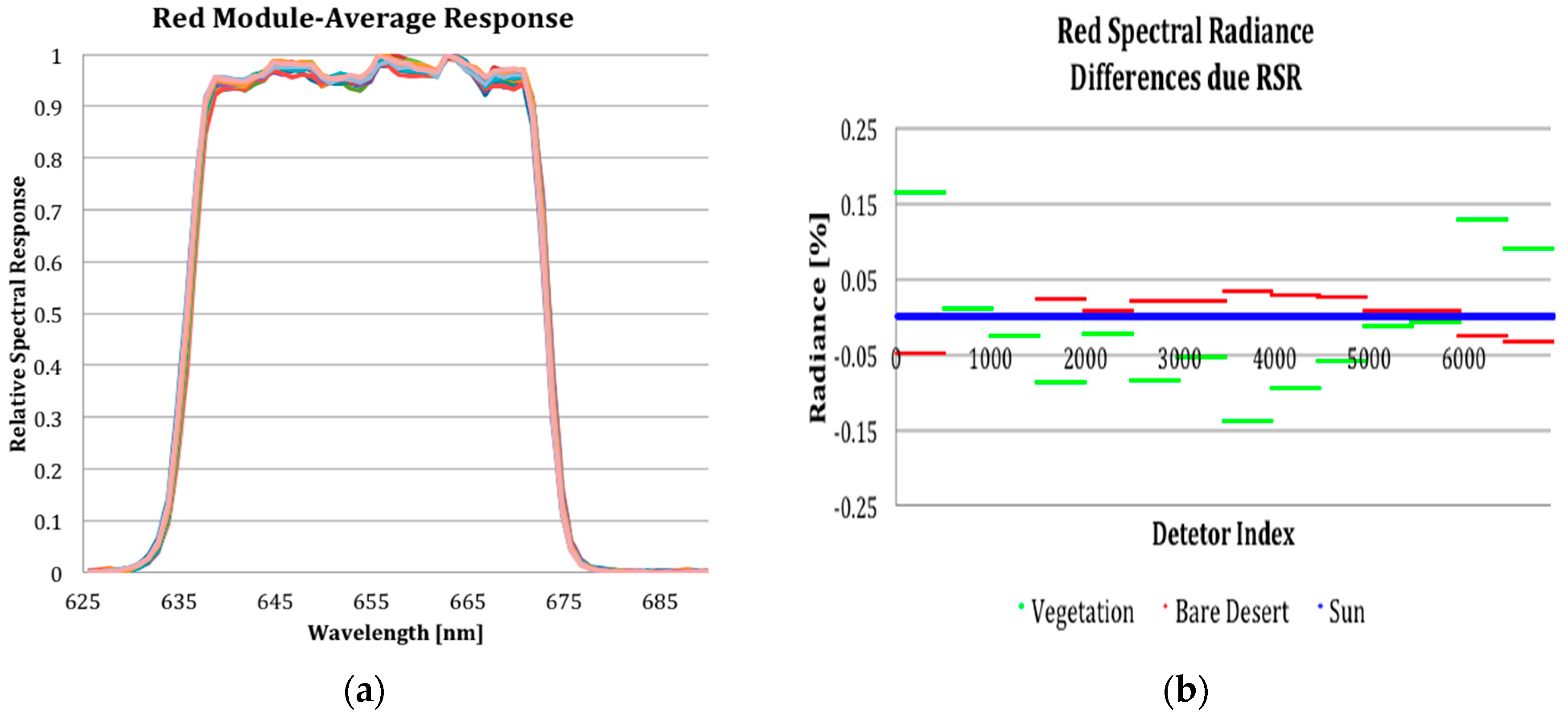
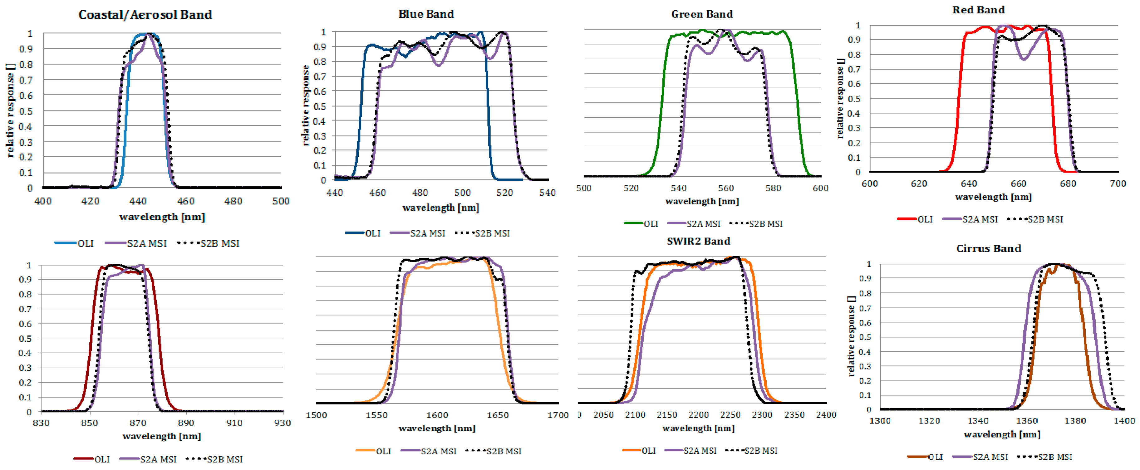
2.2. Spectral Characterization

The spectral characterization of the OLI was strictly a pre-launch operation and is described in detail in Barsi et al. [4]. Three different sets of measurements, component level, FPM level and system level, contribute to the understanding of the spectral response of the instrument. The integrated instrument level measurements, in principle, best represent the true response, although these are sub-aperture, partial field and with weak signals, so out-of-band and crosstalk are not captured. What can be observed at the integrated instrument level are the small shifts in the spectral response across the focal plane due to the slight non-telecentricity of the telescope (Figure 1a). The shifts cause small differences in the responses across the focal plane depending on the spectral shape of the target (Figure 1b). In the example, the vegetated target has a spectral shape that results in more response variability across the focal plane (although < ±0.2%) than the bare desert target. The band average integrated instrument spectral response measurements are published at: https://landsat.gsfc.nasa.gov/preliminary-spectral-response-of-the-operational-land-imager-in-band-band-average-relative-spectral-response/.

Spectral consistency in long-term data records is one of the bigger challenges in providing harmonized data. Even though technologies and sensors continue to evolve, perfectly consistent data are not obtainable. Although spectral adjustment factors can be derived to better match two (or more) sensors’ data, these factors are target- and atmospheric-dependent, meaning that to accurately calculate them one needs to know the signature of the target and atmosphere in advance, which is clearly not the norm in remote sensing.

More consistency and characterization in future sensors can help alleviate parts of the problem. Designs with good internal consistency (e.g., telecentric telescopes and inherently more uniform spectral filters) are a good starting point. Instrument-level spectral characterization of the full instrument focal plane will also help in terms of understanding the true spectral response. Selecting common spectral bands is probably the most useful approach for improving interoperability as any adjustments between systems would be small and would generate small additional uncertainties in the time series.

2.3. Prelaunch Radiometric Characterization and Calibration

The radiometric calibration and characterization of the OLI instrument, both in the pre-launch and on-orbit realms, has been well documented [5,6]. The OLI, as indicated, has extensive on-board radiometric calibration capabilities that allow tracking its performance on-orbit. These capabilities by themselves do not ensure low uncertainty in the radiometric calibration of the instrument; key pre-launch characterizations also required include instrument stability, linearity and non-uniformity, and the calibrators’ radiometric and geometric properties.

The OLI was radiometrically calibrated prior to launch relative to radiance standards traceable to the National Institute of Standards and Technology (NIST) [5]. This calibration is available within the data products. However, uncertainty calculations indicate that a more accurate radiometric calibration can be obtained using the reflectance based approach. This approach relies on the knowledge of the reflectance of the on-board diffuser along with knowledge of the illumination and viewing geometry of this diffuser. The University of Arizona measured the diffuser reflectance at multiple-view angles, illumination angles and locations to reflect the geometric conditions of use.

The estimated uncertainty in the reflectance-based calibration (

Table 3. OLI reflectance-based calibration uncertainty (modified Ball Aerospace table).

Term	Uncertainty (1σ)
	CA	Blue	Green	Red	NIR	SWIR1	SWIR 2	Pan	Cirrus
Initial Diffuser BRDF	1.4%	1.3%	1.1%	1.0%	1.0%	1.7%	1.4%	1.1%	1.7%
Diffuser Geometry	0.9%	0.9%	0.9%	0.9%	0.9%	0.9%	0.9%	0.9%	0.9%
Diffuser Stray Light	0.7%	0.7%	0.7%	0.7%	0.7%	0.7%	0.7%	0.7%	0.7%
Pristine, Wkg Non-Linearity	0%	0%	0%	0%	0%	0%	0%	0%	0%
Wkg, Scene Non-Linearity	1.0%	1.0%	1.0%	1.0%	1.0%	1.0%	1.0%	1.0%	1.0%
FFOV Non-Uniformity	0.3%	0.2%	0.3%	0.3%	0.3%	0.3%	0.4%	0.3%	0.3%
Long Term Stability	0.1%	0.1%	0.1%	0.0%	0.0%	0.3%	0.2%	0.1%	0.6%
Total	2.1%	1.9%	1.7%	1.7%	1.7%	2.2%	2.0%	1.7%	2.3%

) is about 2%, with the dominant effects being the reflectance measurement uncertainty itself, non-linearity, geometric uncertainty (contributes to illumination angle and view angle uncertainties), and stray light within the diffuser assembly.

2.4. On-Orbit Radiometric Calibration of OLI

Radiometric calibration and characterization of the OLI instrument is accomplished by processing all data through the Landsat Product Generation System (LPGS) or the Image Assessment System (IAS) at the United States Geological Survey (USGS) Earth Resources Observation and Science (EROS) Center. To show the radiometric gain trend through time, the average response from each of the on-board calibrators (working lamp, pristine lamp, backup lamp, working solar diffuser and pristine diffuser) were normalized to a point in time shortly after launch. Figure 2 shows the radiometric gain trend over time. Only the coastal aerosol (~1.5%) and blue (~0.3%) bands show any significant change in gain over almost five years on-orbit.

The on-board calibrators provide a very precise trend of the changes in the instrument response, but any connection to the absolute radiometric accuracy is tied back to a NIST reference through pre-launch calibration. In order to get on-orbit validation of this pre-launch calibration, vicarious methods are used [7] as provided by the University of Arizona and South Dakota State University (SDSU). While the vicarious results are not precise enough (~3–5%) to identify small errors or short-term trends, the results provide a measure of the absolute radiometric accuracy and enable long-term gain adjustments [8]. The University of Arizona developed an automated radiometric calibration test site (RadCatS), deployed in Railroad Valley, Nevada, that provides surface measurements continuously throughout the day [9].

2.5. Landsat-8 Geometric Calibration

For the Landsat-8 mission, geometric calibration refers to the process of measuring key elements of the OLI and Thermal Infrared Sensor (TIRS) sensor line-of-sight models to ensure accurate pointing knowledge. These calibration parameters may be sensor characteristics, for example, relative spectral band alignment or sensor chip placement, or they may capture the relationship between the sensor and the observatory, for example the OLI sensor’s attitude control system alignment. The geometric parameters that make up the sensor model were measured during instrument and observatory prelaunch integration and testing. These measurements were used to construct the at-launch sensor line-of-sight model. The prelaunch geometric calibration was refined during the on-orbit observatory commissioning period immediately following launch [10]. This was necessary since some geometric characteristics can change between the ground test and on-orbit operation environments due, for example, to launch shift and zero-G release; and because many of the critical angular parameters can be measured more accurately on-orbit due to the long lever arm when viewing Earth targets as compared to prelaunch laboratory measurements. The on-orbit geometric calibration parameters and resulting calibrated OLI and TIRS sensor models were released for operational product generation at the end of the commissioning period. These parameters are evaluated and adjusted as needed subsequently, based upon an ongoing performance characterization and calibration monitoring activity.

2.5.1. Geometric Calibration Parameters

Table 4. OLI geometric calibration operations and parameters.

Operation	Parameter	Purpose	Frequency
OLI Sensor Alignment	OLI to attitude control system alignment matrix	Estimate OLI orientation relative to attitude control system to improve absolute pointing knowledge/geolocation.	During commissioning. Update quarterly as needed.
OLI Focal Plane Alignment	Pan band sensor chip lines-of-sight	Estimate corrections to pan band line-of-sight model for each sensor chip assembly to improve internal alignment of sensor modules.	During commissioning. Monitor and update if needed.
OLI Band Alignment	MS band sensor chip lines-of-sight	Estimate corrections to MS band line-of-sight models to improve band-to-band alignment, holding pan band fixed.	During commissioning. Monitor and update if needed.

summarizes the geometric calibration parameters that are maintained on-orbit for the OLI. The table identifies the calibration operation that is used to update each parameter, and briefly describes the purpose and frequency of each calibration. These parameters can be adjusted to improve internal image geometry (focal plane alignment), band registration accuracy (band alignment), and absolute geolocation accuracy (sensor alignment).

Prior to launch, it was expected that all parameters would require some fine-tuning during commissioning but that only the OLI sensor to spacecraft attitude control system (ACS) alignment would be likely to require subsequent, possibly seasonal, adjustment during normal operations. This has been confirmed by events with only two minor calibration parameter adjustments (in July 2013 and February 2014), both to the OLI-to-ACS alignment, having been applied since the end of commissioning. This stable calibration has made it possible to achieve absolute geolocation accuracy of 18 m (CE90) for the duration of the mission to date [10].

2.5.2. Calibration, Reference Data, and Interoperability

An important additional factor in Landsat-8 OLI product geometric accuracy is the use of ground control points during product generation to ensure multi-temporal registration for products throughout the Landsat archive. These control points were originally derived from the Global Land Survey (GLS) data set composed of Landsat 7 data circa 2000 [10]. The use of ground control for registration can be thought of as a type of per-product calibration wherein the ground control points serve as the calibration standard. The geometric accuracy of Landsat-8 products is thus dependent upon the accuracy of the control point standard as much as or more than the inherent accuracy of the calibrated Landsat-8 OLI system. The accuracy of the GLS framework is estimated to be 25.8 m (CE90) so, for Landsat-8, the use of ground control to achieve multi-temporal consistency negatively affects absolute product accuracy. Although it ensures registration accuracy within the Landsat archive, the GLS control limits registration accuracy to other data sets, such as Sentinel-2, that are not tied to the GLS framework.

Direct comparison of Landsat-8 and Sentinel-2 data at 317 globally distributed test sites, with locations shown in Figure 3, resulted in a measured registration accuracy of 22.9 m (2 σ). This is somewhat better than might have been expected given the estimated accuracy of the GLS framework, but it is still more than two-thirds of an OLI multi-spectral pixel. Significantly better registration accuracy is required to allow Landsat-8 and Sentinel-2 data to effectively interoperate. A global re-triangulation of the GLS control framework is underway using Landsat-8 data to improve the consistency and accuracy of the global control reference [11]. The triangulation will include tie points extracted from the Sentinel-2 global reference image (GRI) to make the two frameworks consistent and improve registration accuracy and interoperability. Completion is expected in early 2019 to support a complete Collection-2 reprocessing of the Landsat archive.

3. Calibration Status of Sentinel-2

3.1. Sensor Description

As part of the Copernicus program of the European Union (EU), the European Space Agency (ESA) has developed and is currently operating the Sentinel-2 mission acquiring high spatial resolution (10 to 60 m) optical imagery. The Sentinel-2 mission concept draws in large part from the heritage of the Landsat program, as well as from the French Satellite Pour l’ Observation de la Terre (SPOT) series.

The Sentinel-2 mission is performed by 2 identical satellites (S2A, launched in June 2015, and S2B, launched in March 2017) each carrying a single imaging payload named MSI (the Multi-Spectral Instrument). Thanks to a wide imaging swath of 295 km, the two satellites ensure a revisit time of 5 days over a large part of global emerged lands and coastal waters, producing some 4 Terabytes of data every day.

The MSI is a pushbroom imager with a three-mirror anastigmat design utilizing 10 focal plane modules forming 10 bands in the visible and near-infrared (VNIR) and 3 bands in the SWIR (see [12] for a complete description). A solar diffuser can be positioned at the entry of the telescope for radiometric calibration purposes. Unlike OLI, the MSI does not accommodate an additional reference diffuser or calibration lamps.

3.2. Radiometric Calibration

Use of the onboard solar diffuser is the principle absolute radiometric calibration approach and is fully described in [2]. The solar diffuser provides a bright and uniform image of the solar illumination, for which the incoming solar irradiance is well known based upon use of a relevant solar spectrum irradiance (Thuillier model recommended by the Committee on Earth Observation Satellites (CEOS) [13]) convoluted by the spectral band definitions, and accounting for a fine Earth–Sun distance calculation (based on Orekit [14]). As with Landsat OLI, knowledge of the detailed solar-diffuser bidirectional reflectance distribution function (BRDF) is the most sensitive point of the calibration method. A refined diffuser BRDF that fits a Rahman model better characterizes the diffuser panel. The overall gain trend for Sentinel 2 A and B are shown in Figure 4.

The radiometric sensitivity of Sentinel-2 MSI presents a slight decrease with time. The absolute gain coefficients decrease by about 0.1% to 0.4% for S2B over six months in space, depending on the spectral band (Figure 4, use of the refined BRDF). For S2A, the trend of sensitivity loss reaches 0.4 to 1.0% over two years and half in orbit.

Validation of the absolute calibration is based on vicarious measurements. Many methods are applied: the Rayleigh calibration method, the desert (PICS) calibration method, the in situ calibration method, and the inter-sensor calibration method. These methods are fully discussed in [2,15].

The Rayleigh calibration method is based on the comparison of the observed atmospheric molecular scattering over oceans with simulations. It allows an absolute calibration of the shortwave bands, from blue (B01) to red (B04). The desert calibration method is performed over 6 CEOS PICS in North Africa (http://calvalportal.ceos.org): bright sites, spatially uniform and mainly very stable over time. This calibration method is based, too, on simulation of the observations [16]. The in situ calibration method is a collaborative task between the University of Arizona, the National Aeronautics and Space Administration (NASA) and S2-MPC using the well-known Railroad Valley calibration site in Nevada.

Figure 5 illustrates the results for the spectral bands of MSI-A and MSI-B. Discrepancies between the different methods are lower than 5%, which is in the range of the Sentinel-2 specifications. The desert PICS validation method shows a consistency of the absolute calibration with discrepancies even lower than 3% for all the bands, except the 705 nm band for MSI-A. Results for the in situ validation, over the Railroad Valley site, are in the same range of discrepancies. For the Rayleigh calibration, a 4% discrepancy is obtained at the maximum for the B01 band, centered at 440 nm. In this spectral range, even if the Rayleigh scattering is the strongest, the sensitivity of the method to an uncertainty on the water reflectance is important.

One can also notice the MSI-B reflectance is lower than the MSI-A reflectance for VNIR bands (see green squares on the bottom plots in Figure 5). The discrepancy is about 1% for most of the VNIR bands.

Complementary analysis to improve the calibration approaches for better data interoperability of Sentinel-2 and Landsat-8 could be (i) to confirm their calibrations are computed with the same solar irradiance model and Earth–Sun distance; (ii) to increase, from both NASA and ESA, the amount of vicarious calibrations over the same sites, using the same spectral characterization of the targets, the same atmospheric parameters, the same radiative transfer code, as well as quasi-simultaneous observations.

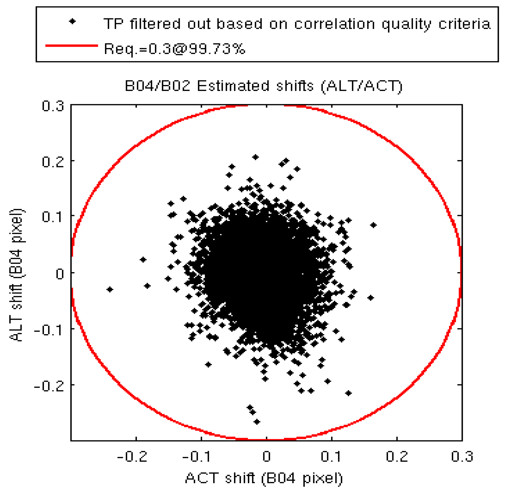
3.3. Geometric Calibration

Geometric calibration activities aim to fulfill and validate the following mission requirements:

• absolute geolocation performance better than 12.5 m (circular error at 95%);
• multi-temporal relative geolocation accuracy better 3 m (circular error at 95%);
• relative co-registration between any pair of spectral bands better than 0.3 pixel of the coarser spatial sampling distance (circular error at 99.7%).

Calibration activities include:

• calibration of the relative viewing directions of each detector pixel;
• adjustment of on-board time lag;
• monitoring and adjustment of the spacecraft line-of-sight model;
• image geometric refinement using a global reference image.

The first two activities were performed during the commissioning period of each S2A and S2B unit, and no subsequent adjustment was made.

The multispectral registration performance is continuously monitored: a degraded performance could indicate the need to recalibrate the line of sight. The method uses cloud-free images over flat terrain. Matching image patches between different spectral bands are identified and the shift vectors are computed. Point cloud plots are produced to identify potential biases (see Figure 6 below) and along-track Fourier transform of the error is used to detect potential oscillations in the line of sight.

The third activity is to determine the three rotation angles (roll, pitch, yaw) characterizing the pointing bias of the instrument reference line-of-sight with respect to the Attitude and Orbit Control System (AOCS) frame. These angles are still evolving for both satellites.

The absolute geolocation performance is constantly monitored using a set of ground control points around the globe. Every month, approximately, the point cloud of errors is plotted in the along-track/across-track frame. If the cloud shows a bias in the along-track (respectively across-track) direction, a calibration of the pitch (respectively roll) angle is required. The yaw angle is more difficult to monitor; a yaw bias can be detected by looking at the variation of the along-track error component along the swath.

To compute the new calibration angles, images in the sensor frame (L1B) and another set of ground control points is used. The angles are obtained by minimizing the global error over the set of control points.

In the near future, a similar procedure will be performed to refine the geometric model of all Sentinel-2 images. The geometric refinement process uses as a reference a set of carefully georeferenced images, the GRI. For each image data strip, the viewing model will be adjusted to minimize the shift between the current image and the reference image. This procedure and the associated Global Reference Image are currently being validated. Aligning all images with the same GRI is expected to reduce the multi-temporal error from 12 m today to less than 3 m.

4. Calibration Comparison of Landsat 8 and Sentinel 2

Several university teams have been acquiring Landsat 8 and Sentinel 2 data since the launch of each instrument for the purposes of vicarious calibration [17,18,19]. Additionally, two groups have developed absolute calibration models for PICS that can be used for both OLI and MSI. Initial work comparing Landsat-8 OLI and Sentinel-2A MSI follows; more details on the study can be found in Barsi et al. [20].

Because the two instruments have significant overlap in spectral bandpasses (see Figure 7), these differences must be accounted for through use of a spectral band adjustment factor (SBAF; [21]). The SBAF is target specific and requires a source of hyperspectral image data to calculate. Using the SBAF, the MSI reflectances can be converted to OLI equivalent reflectances.

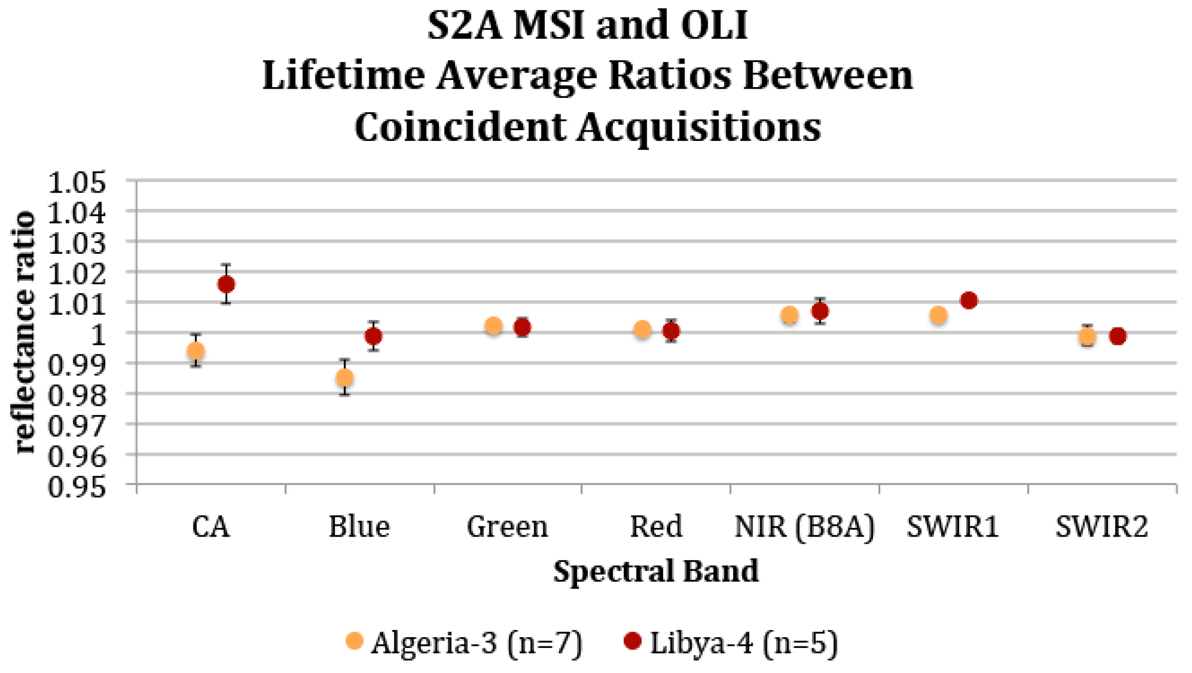
4.1. Calibration Comparison Using Coincident Acquisitions

Due to the orbital properties of Sentinel-2 and Landsat-8, the instruments acquire coincident images of specific locations on Earth every 80 days. For Sentinel-2A, two of these locations happen to be two of the CEOS-defined PICS regions [22], long used for instrument calibrations: Libya-4 and Algeria-3. Since the launch of Sentinel-2A, the instruments have acquired 5 cloud-free images of Libya-4 and 7 of Algeria-3. For these image pairs, the top-of-atmosphere reflectance can be directly compared once accounting for the spectral band differences and the solar zenith angles. Figure 8 shows the ratios between the lifetime average top-of-atmosphere (TOA) reflectance between OLI and MSI for the common spectral bands. In general, the instruments agree to within 1%. There is less agreement in CA and Blue bands; though the instruments agree to within 1.5%, the differences between the sites are larger. In the CA and Blue, the reflectance differences are consistent to within 0.7% (1-sigma) for a given site. This suggests that there are still some spectral differences that are not accounted for in the SBAF correction.

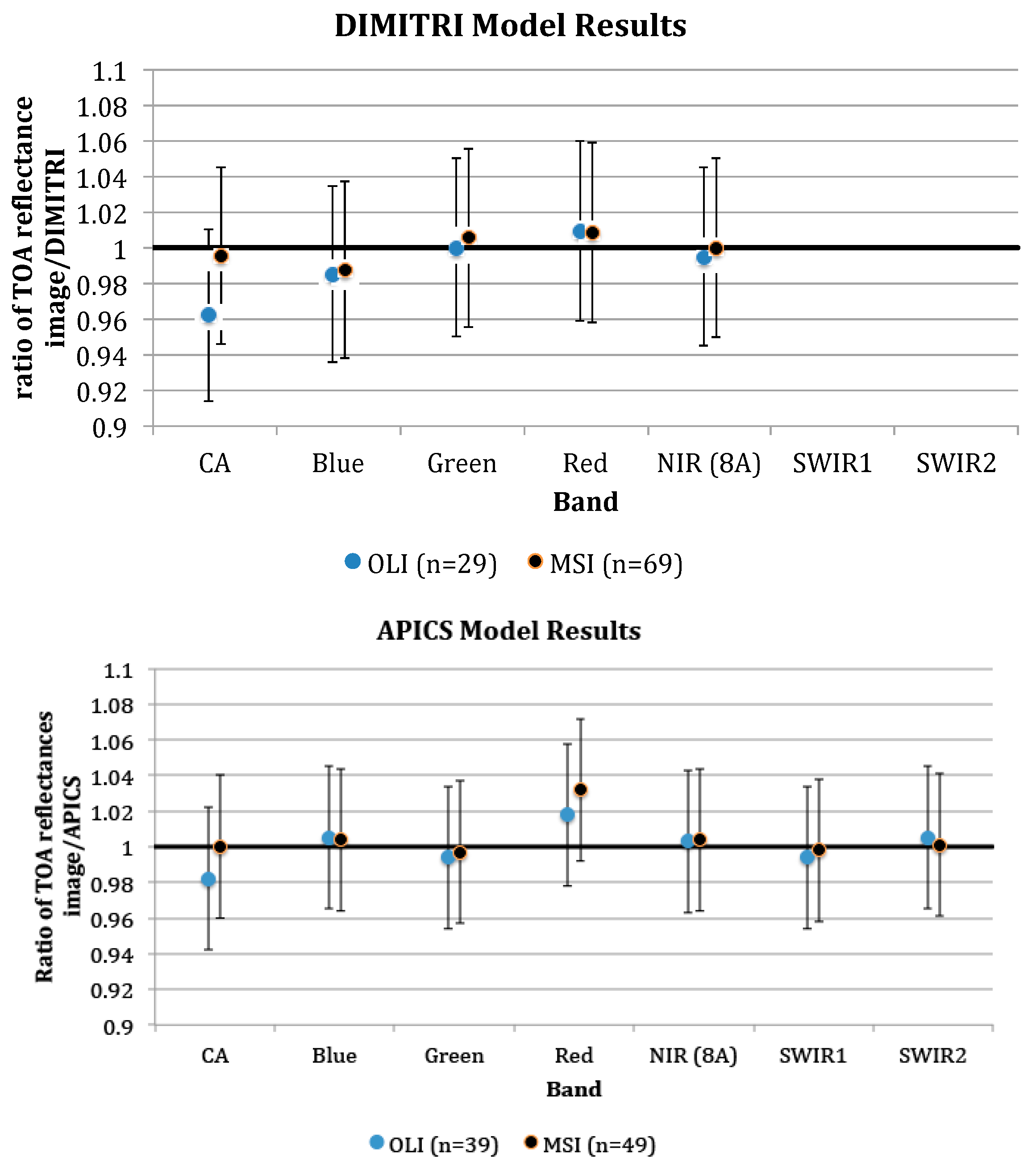
4.2. Pseudo Invariant Calibration Sites (PICS) Absolute Calibration Based on Hyperspectral Sensor Models

Two different models are being used to predict the TOA reflectance of the PICS regions using hyperspectral satellite data as the source of the “field” data. The models consider the atmospheric conditions, BRDF, and solar and viewing geometries in converting hyperspectral TOA reflectances to multispectral TOA reflectances (either OLI or MSI bandpasses). The South Dakota State University Absolute PICS (APICS) model uses Hyperion data [23], and the ESA Database for Imaging Multi-spectral Instruments and Tools for Radiometric Intercomparison (DIMITRI)-PICS model uses Medium Resolution Imaging Spectrometer (MERIS) data [16]. Results using these models are shown in Figure 9 and indicate that the two instruments are calibrated to within 2% of each other, except for possibly the CA band.

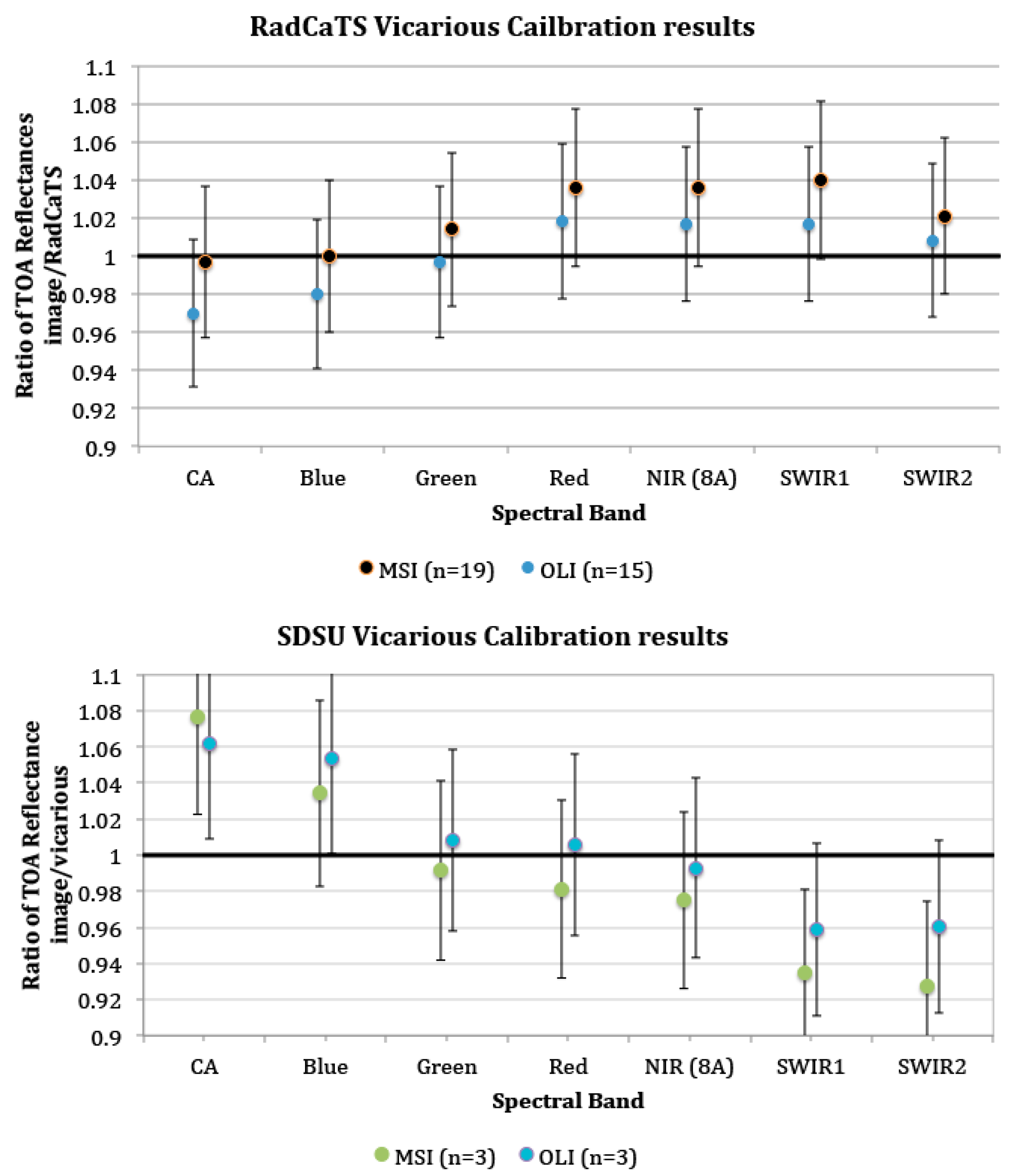
4.3. Vicarious Calibration Based on In Situ Surface Measurements

Two teams in the United States have been acquiring reflectance measurements of the surface under OLI and MSI: University of Arizona (UAz) at the Railroad Valley Playa, Nevada (RRV), and South Dakota State University (SDSU) at the Brookings, SD, site [24,25]. In both cases, the software MODTRAN (Moderate Resolution Atmospheric Transmission) is used to predict top-of-atmosphere reflectance from the surface measurements, which are then compared to the reflectance measured by OLI and MSI. See Figure 10. Results of these calibration efforts suggest, once again, that the two instruments are calibrated consistently with respect to each other in the order of 2% or better. However, absolute calibration uncertainties are somewhat larger, though consistent within their respective methodologies.

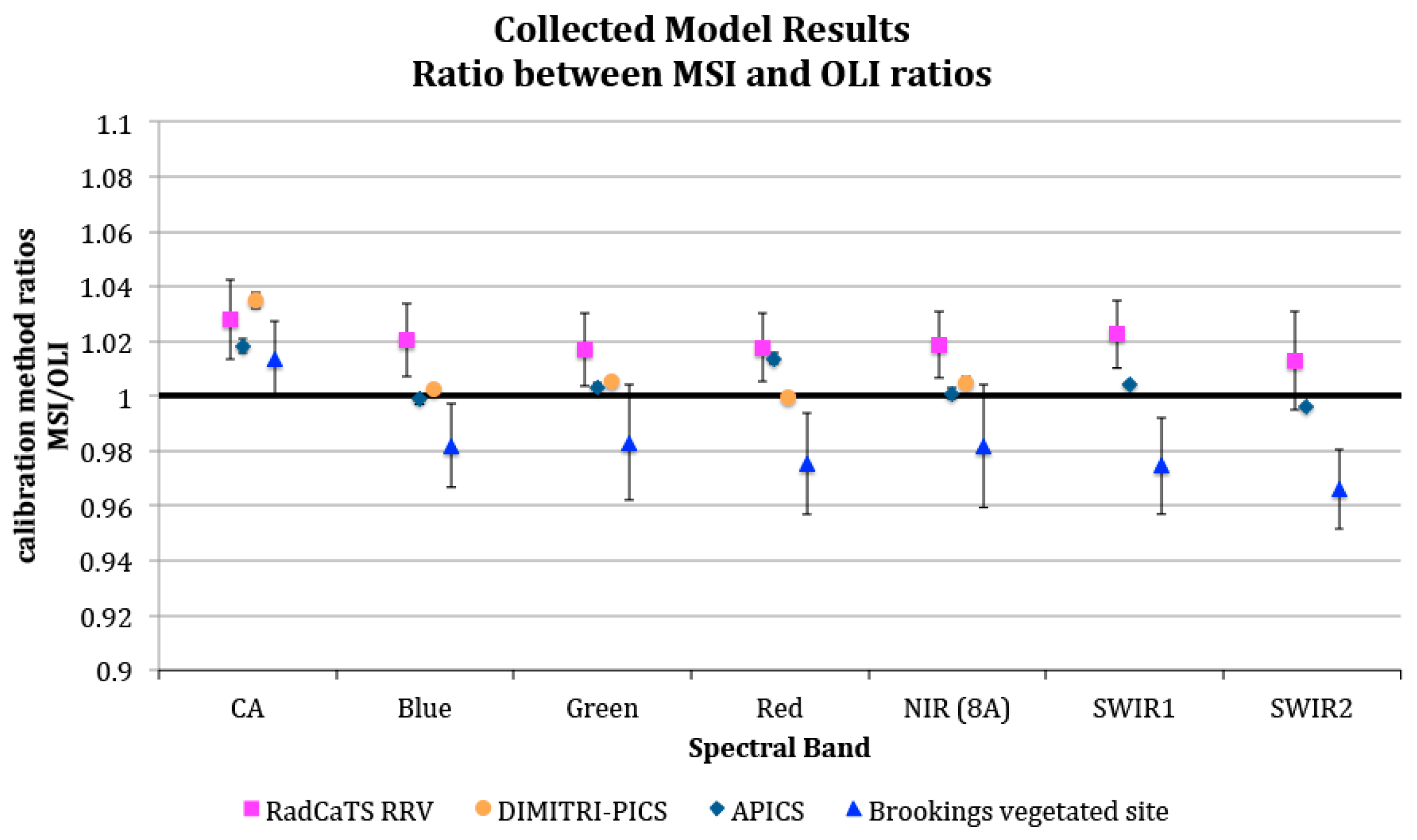
4.4. Summary of Results

In order to combine all methods of validating the calibration of MSI with OLI, the ratios of the MSI and OLI results are taken. This metric should serve to remove any systematic errors within the models and provide for a per-model comparison of OLI and MSI. Results are shown in Figure 11. The DIMITRI-PICS model predicts that OLI and MSI are within 1% for all VNIR bands except the CA, which is likely due to the use of Landsat pre-collection data. The APICS model indicates the instruments are within 2% for all bands. The UAz RRV comparison shows that MSI and OLI are within 2% across all bands, though with MSI consistently brighter than OLI. Even the SDSU vicarious results, which indicate the largest absolute calibration errors, suggest the instruments are calibrated to within 4% of each other.

5. Current Status and Limitations of Data Interoperability with Landsat and Sentinel

Since 2015, a number of researchers have worked to combine Landsat and Sentinel-2 data for particular applications, and more efforts to do so are emerging on a regular basis. In this section we provide the perspective from several applications research groups on the current status and limitations of interoperability between Landsat and Sentinel-2, and the expectations emerging from the broader international Earth observation community. These perspectives, in conjunction with the calibration results above, inform the recommendations for the calibration community provided in Section 6 below.

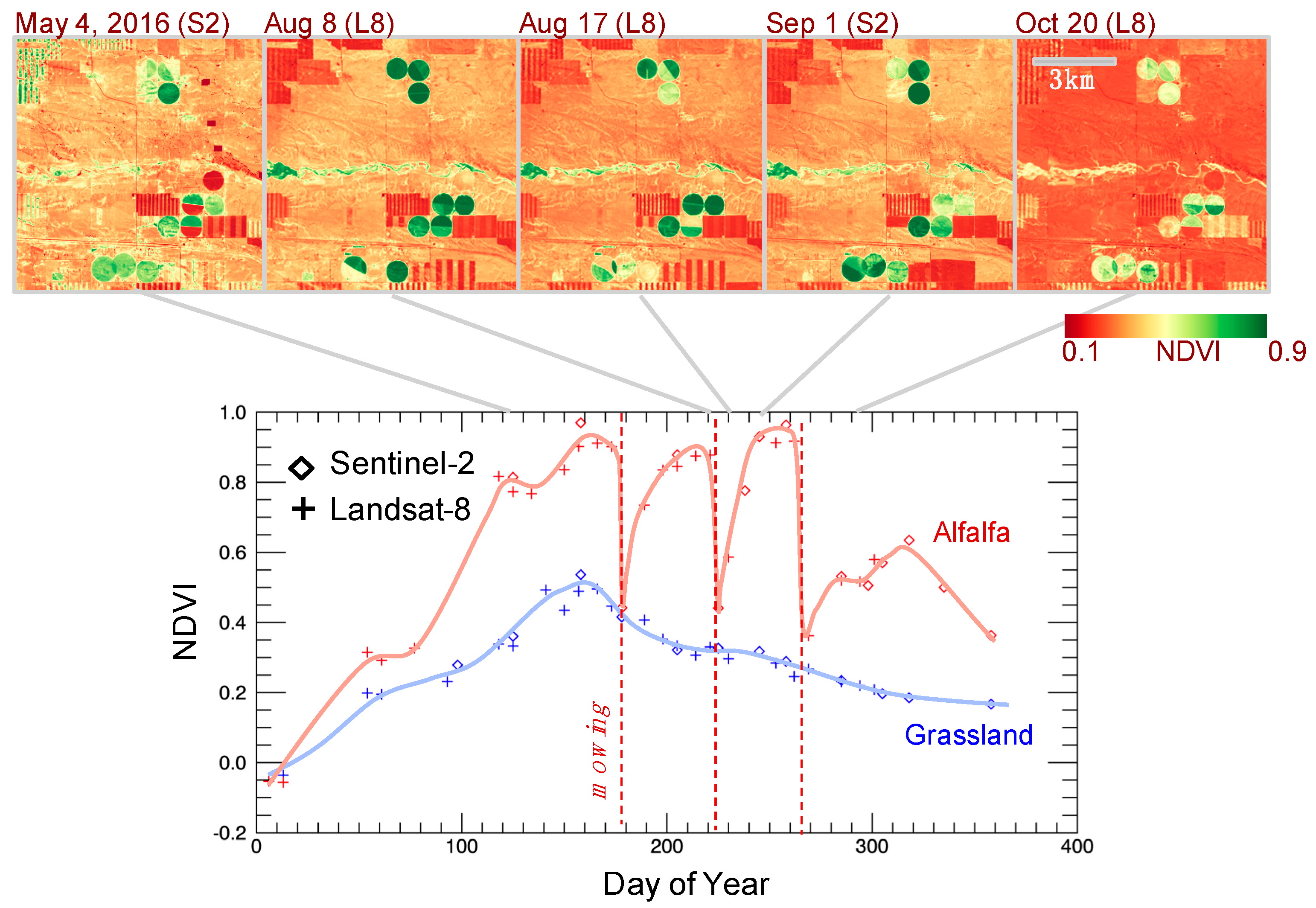
5.1. Harmonized Landsat/Sentinel-2 (HLS) Project

The NASA Harmonized Landsat/Sentinel-2 (HLS) Project has been working to create a seamless surface reflectance record using input data from Landsat 8 OLI and Sentinel-2A/B MSI. In this context, “harmonized” means that that sensor-specific radiometric and geometric differences are adjusted and removed, such that it should be transparent to end users which sensor originated any specific reflectance observation within an HLS time series. Specifically, the HLS processing stream includes a common atmospheric correction for each sensor based on the Landsat 8 Surface Reflectance Code (LaSRC) approach [26], BRDF adjustment to nadir view angle and constant solar elevation [27,28], spectral bandpass adjustment of Sentinel-2 MSI to better match Landsat 8 OLI, and cloud and shadow masking. HLS products are geo-registered to Sentinel-2 clear images, and regridded using the Sentinel-2 Universal Transverse Mercator (UTM) tiling system at 30-m resolution. The overall goal is to create dense time series of reflectance observations suitable for use in mapping highly dynamic surface processes, including crop type, condition, and management practice, vegetation phenology, and surface water extent (Figure 12).

To date, the HLS project has not directly evaluated how calibration uncertainty in Level 1 inputs propagates to output reflectance time series. In part, this reflects initial findings from the NASA/USGS and ESA instrument teams reporting that each sensor met its own calibration requirements, and that their radiometric responses were comparable within measurement uncertainties [20]. Instead, the main effort has gone toward assessing the absolute reflectance uncertainty of HLS products, and assessing short-term temporal stability (using reflectance retrievals from pseudo-invariant calibration sites or PICS). Short-term relative reflectance variability evaluated from bright PICS sites are generally in the range of ~3% for both visible and near-infrared bands. Residual variability is likely due to a combination of unmasked thin clouds, errors in aerosol retrieval, errors in the BRDF adjustment, and errors in the spectral bandpass adjustment, in roughly that order.

Assessment of absolute accuracy for HLS products has relied on independent studies of the LaSRC atmospheric correction, as well as comparisons with Moderate Resolution Imaging Spectrometer (MODIS) nadir-adjusted products and in situ data collected by Surface Radiation Budget Network (SURFRAD) broadband radiometers [29]. The LaSRC algorithms for Landsat 8 and Sentinel-2 have been validated by comparing output surface reflectance with results derived from running the 6S radiative transfer model using aerosol inputs from in situ AERONET (Aerosol Robotic Network) measurements. These comparisons indicate absolute surface uncertainty (root-mean-square error (RMSE)) varying from ~0.006 (darker targets) to 0.009 (bright targets), which convert to relative errors of 2–6%. Comparisons with SURFRAD indicate higher uncertainties, with RMSE of ~0.02 or ~10% relative. It should be noted that these validation approaches do not measure the same sources of error. The AERONET comparisons only include errors associated with the LaSRC image-based aerosol retrieval, while the SURFRAD comparisons include the full range of HLS processing. At the same time, the SURFAD measurements require HLS spectral reflectance values to be interpolated to broader spectral bandpasses, which is another potential source of error. A key point is that the land remote sensing community still lacks an established network of ground observations of surface spectral reflectance for use in validating moderate-resolution products such as HLS.

The HLS project has encountered several other challenges in generating harmonized products. These include:

• Sensor misregistration: as noted above, Landsat 8 ground control differs from Sentinel-2. To minimize image-to-image variability when stacked as time series, HLS has implemented an approach whereby each Landsat image is co-registered to a “master” Sentinel-2a image using image cross-correlation techniques [30].
• Cloud masking: in the absence of a thermal channel, it has proven difficult to generate reliable cloud masks for Sentinel-2 imagery. Currently, the HLS project uses the output of the LaSRC cloud mask combined with the Boston University Fmask algorithm [31,32].
• Processing baselines: in 2017 USGS moved from the earlier L1T product to the “Collection 1” products, and announced plans to make analysis ready data (ARD) the default product by the launch of Landsat 9 in 2020. Similarly, ESA evolved the L1C baseline processing over several iterations during the early phases of the Sentinel-2 mission, including changes to the product filename and file structure. While welcome, these changes have made it difficult to standardize and synchronize the HLS processing. In addition, ESA has not yet implemented a “collection” model that includes archive-scale reprocessing.

To date, HLS has generated products covering some 9.1 million km², or about 7% of the global land area. The project is planning to release a wall-to-wall North America product, with <5 day latency, during calendar year 2018. Additional details on the HLS processing and current status of the product suite can be found on the project web site: https://hls.gsfc.nasa.gov.

5.2. Landsat-8 and Sentinel-2 Burned Area Mapping

Mapping the spatial extent of fire-affected areas on a systematic basis is needed in support of numerous science applications, and in particular for estimation of pyrogenic emissions of greenhouse gasses and aerosols. Landsat data have been used for burned area mapping since the availability of the first Landsat 1 data [33,34]. However, Landsat-based burned area mapping is significantly limited by the low Landsat temporal revisit, combined with cloud cover, and, in many regions, by rapid post-fire vegetation regrowth and dissipation of char and ash [35,36]. In the last two decades global burned products have been produced using coarse spatial resolution data [37], notably, using change detection algorithms that take advantage of the near daily MODIS 500 m observation record [38,39]. The Sentinel-2 MSI has spectral bands that are well suited for burned area mapping [40] and with Landsat 8 OLI provide the opportunity for medium-resolution burned area mapping using change detection algorithms, particularly as both Sentinel-2 data streams with Landsat 8 provide a global median average revisit interval of 2.9 days [41].

As noted for the HLS project, there are a number of pre-processing issues required before Landsat-8 OLI and Sentinel-2 MSI data can be used seamlessly together. Significant progress has been made, however, although there are still ongoing issues. This is illustrated briefly below in support of a NASA-funded project to develop burned area products using Collection 1 Landsat 8 OLI and Sentinel-2 MSI data. Rather than use the Sentinel-2 MSI tiling system, that is complex to use for large area applications as adjacent tiles from the same MSI swath overlap spatially and may be defined in different UTM zones [42], both sensor’s data are reprojected into the MODIS sinusoidal projection [43]. In this way, the reprojected data are straightforward to compare with the standard MODIS land products (e.g., [44]) and burned area estimates are defined without areal bias as the MODIS projection is an equal area projection. The Sentinel-2 and the Landsat-8 data are registered to sub-pixel precision using affine transformations derived with a robust matching algorithm developed for this purpose [45] and via a least-squares adjustment among different orbits to reduce sensitivity to missing and cloudy data typically found when registering only individual tiles and images [46]. Research to downscale Landsat 8 30 m data to 20 m Sentinel 2 MSI resolution is underway [47] but currently the MSI 20 m data are upscaled to 30 m by bilinear resampling and the Landsat 8 Collection1 data are also bilinear resampled.

Both sensor’s data are atmospherically corrected using the LaSRC algorithm as described above for the HLS data. The Landsat-8 Collection 1 cloud mask [48] is used to discard cloud-contaminated pixels. The Sentinel-2 L1C cloud mask currently performs poorly, and instead the SEN2COR cloud mask [49] is used for Sentinel-2 application. Research to evaluate shadow masks in the Landsat-8 Collection 1 and Sentinel-2 L1C products is underway. Bi-directional reflectance variations imposed by variations in the viewing and solar geometry occur over most terrestrial surfaces and, for many applications, are considered as a source of noise. Surface reflectance anisotropy, has been observed to cause NIR reflectance variations up to 0.06 (reflectance units) across the Landsat swath [27] and up to 0.08 across the Sentinel-2 swath [28]. Although these variations are much smaller than observed for MODIS data, where they can be greater than reflectance changes due to biomass burning [50], they are still not insignificant. Therefore, the surface reflectance data are corrected to nadir BRDF-adjusted reflectance (NBAR) using a semi-empirical c-factor approach that provides a first-order BRDF correction [27,28].

Figure 13 shows a time series of Landsat 8 OLI (filled circles) and Sentinel-2A MSI (open circles) surface NBAR data processed as described in the above two paragraphs for a single 30 m location. The near-infrared (865 nm) and short-wave infrared (1610 nm) bands of each sensor are illustrated as these bands are sensitive to fire effects [34,40,50]. The pixel is over a Zambian woody savanna location and burned after day 208 and on or before day 214, with evident drops in OLI and MSI surface NBAR between these dates.

In Figure 13 it is apparent that OLI and MSI observations were acquired occasionally on the same day or only one day apart but that their surface NBAR values are different, despite the above processing. On the same day different sensor acquisitions were within 15 min of each other and so it is unlikely that the observed differences were due to surface or atmospheric changes. Rather they are due to sensor spectral band pass differences and residual calibration, atmospheric correction and NBAR derivation errors. A statistical comparison of a large amount of OLI and MSI surface NBAR data, similar to the approach applied to derive statistical spectral transformations between Landsat 7 and Landsat 8 data [51], has been undertaken. The MSI surface NBAR MSI data were adjusted to OLI using the spectral linear transformations [52] and evidently (straight lines) make the plotted OLI and MSI surface NBAR time series more coherent with respect to each other.

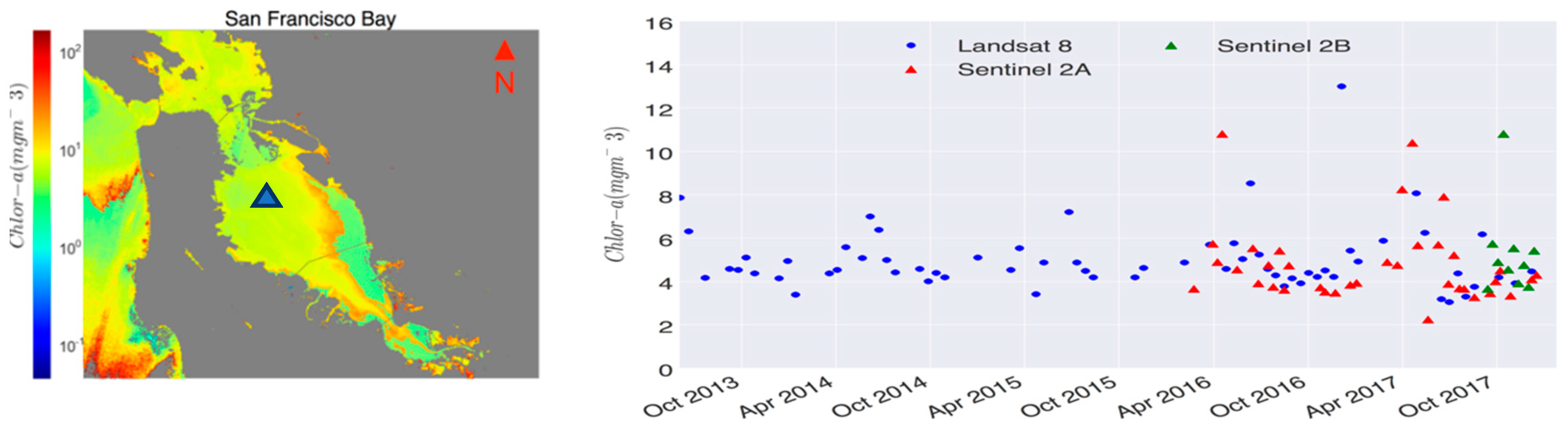
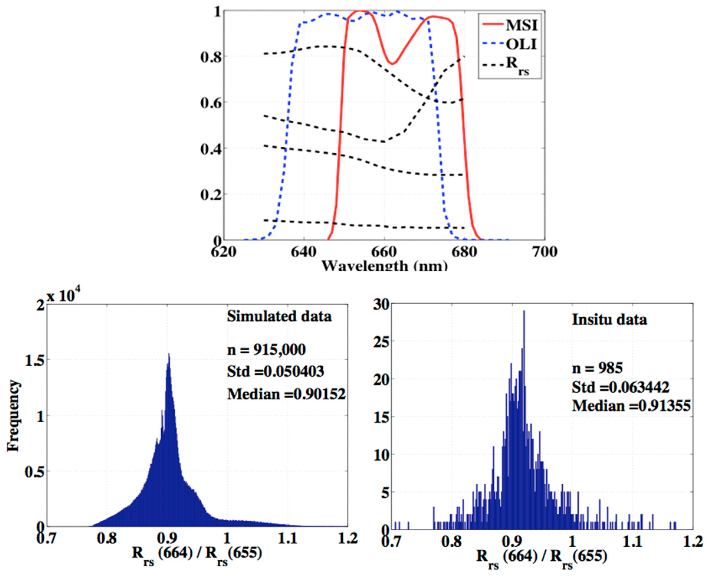
5.3. Aquatic Applications: Potentials and Limitations

Within the next decade, the Landsat-8 and Sentinel-2 virtual constellation will be the primary source of well-monitored Earth-observing datasets for monitoring water resources, including lakes, reservoirs, rivers, bays, and other nearshore coastal areas. Because of the improvements in the sensor technology, the image data from this constellation was anticipated to outperform heritage missions like Landsat-5 and -7 [53,54,55] or the SPOT. The primary advantages come from (a) the improved SNR and (b) the additional spectral bands at ~443 nm and within the NIR region. The high data quality together with 2.9-day revisit time of the constellation revolutionizes the way satellite data are utilized for science algorithm development and/or monitoring applications in inland and nearshore coastal waters. For either purpose, consistency in both TOA and atmospherically corrected products, i.e., remote-sensing reflectance ($R_{rs}$), is critical. The remote-sensing reflectance, defined as the ratio of water-leaving radiance to total downwelling irradiance just above water [56], plays a major role in enabling quantification of water constituents, including the concentrations of total suspended solids (TSS) and chlorophyll-a (Chl), the absorption by colored dissolved organic matter (CDOM), and other products like turbidity, clarity, or Secchi disk depth.

From the ocean color literature, it is well-known that a 1% calibration offset in the blue bands yields a 10% error in $R_{rs}$ over blue ocean waters [57,58]. In optically complex inland/nearshore waters, a 1% calibration offset may translate to larger errors in $R_{rs} (\lambda <500 \mathrm{nm})$ in CDOM-rich waters in the blue bands. It is also possible that the uncertainties may be smaller in extremely eutrophic/turbid waters in $R_{rs} (\lambda >600 \mathrm{nm})$ than those over clear ocean waters in this spectral region. The sensitivity of algorithms to uncertainties in $R_{rs}$ also determines the required accuracies/precision in TOA measurements, i.e., sensitivity to calibration performance may differ for different algorithms. For example, band ratio algorithms [59,60] tend to be less susceptible to uncertainties in $R_{rs}$. An example of a time-series chlorophyll-a product over an arbitrary location (marked by a triangle) in San Francisco Bay is illustrated in Figure 14. The products are derived from Landsat-8, Sentinel-2A, and Sentinel-2B using a blue-green band ratio. Note that while Landsat-8 and Sentinel-2A have been vicariously calibrated, Sentinel-2B data are processed “as is”.

For monitoring applications where anomalies in water quality conditions are sought, such uncertainties are of less importance. However, for science algorithm developments and the associated time-series applications, uncertainties in $R_{rs}$ require major attention. Furthermore, to ensure various global and region-specific algorithms transfer minimal uncertainties to products like Chl or TSS, it is logical to maintain high-quality TOA observations with minimal calibration errors or instrument artifacts. Last, but not least, to enable robust monitoring of water quality indicators, it is essential to provide end-users with per-pixel uncertainty estimates. This goes beyond existing quality assurance (QA) flags and allows for providing a confidence level to each pixel enabling effective decision-making. Such uncertainty products for Landsat-8 and Sentinel-2 are only possible when calibration uncertainties or instrument artifacts are well known. It is, thus, crucial to have accurate knowledge of radiometric performance of this constellation throughout its lifetime.

Currently, preliminary vicarious calibrations [61] conducted for a handful of OLI [62] and MSI images [63] using in situ data autonomously measured at the Marine Optical Buoy (MOBY) and the Buoy for the Long Term Acquisition of Time Series (BOUSSOLE) site have yielded reasonable relative consistencies in TOA, $R_{rs}$, and TSS products. Analyzing the near-simultaneous overpasses after vicarious calibration indicated that the corresponding products agree, on average, within 0.5% in TOA and 8% in using in situ measurements at the MOBY and the BOUSSOLE site with the red channel showing the largest differences. This largest discrepancy in the red channel is attributed to imperfect spectral-band adjustments in the red spectral bands.

Figure 15 illustrates the Relative Spectral Responses (RSRs) (only within 600–700 nm) overlaid onto hyperspectral in situ $R_{rs}$. where shifts in the spectral bands can be inferred [63]. The histograms in Figure 15 show the distributions of the ratios in the red channels, i.e., MSI to OLI, obtained from simulated/measured hyperspectral R_rs data [63]. The spread in the distribution indicates that if a median ratio (~0.9) is chosen for spectral band adjustments, errors are expected in intercomparisons.

Overall, although the existing intercomparison exercise has minimal uncertainties [62,64], there seems to be a need for further improvements in the treatment of differences in red channels in both the TOA and $R_{rs}$ domains. With the foreseeable improvements, it is possible to utilize the approach to ensure consistency in radiometric responses in the future. Such efforts will become more critical as the instruments and onboard calibration devices age. Regardless of the radiometric performance of the instruments, it is worth noting that high-quality products (e.g., Chl) are nearly impossible over areas affected by haze in the sunglint region, i.e., the eastern portion of the scenes. In addition, differences in the SNRs may also contribute to differences in products at local scales, i.e., pixel-level. For instance, band ratio algorithms may accentuate random noise contributions leading to larger discrepancies in the products.

5.4. Data Interoperability for the International Community

The international community, through the Committee on Earth Observation Satellites (CEOS), is expressing an expectation of data interoperability as a general principle, beyond specific application areas such as those discussed above. Interoperability is seen as a key requirement to deliver benefit from operational remote-sensing satellite systems such as Landsat and Sentinel 2, and as a logical ‘next step’ to build on the success of free and open data [65].

CEOS (www.ceos.org) seeks to optimize the benefits of space-based Earth observation through high level cooperation in areas such as mission planning and provision of compatible data products and policies. As applications become more operational, data suppliers will need to ensure:

• Continuity so that down-stream products can be developed with confidence that the data streams will continue, with smooth transitions as old instruments are retired and replaced with newer versions;
• Interoperability between data streams to allow reliable and high-quality products, as demonstrated in the NASA HLS Project; and
• That data are fit for use by specialists in agriculture, security, civil engineering, disaster management and so on, who may not be remote sensing scientists. These users will need data that are ‘ready to use’.

CEOS is therefore establishing a framework for analysis-ready data for land applications, defined as: CEOS Analysis Ready Data for Land (CARD4L) are satellite data that have been processed to a minimum set of requirements and organized into a form that allows immediate analysis with a minimum of additional user effort, and, interoperability both through time and with other datasets.

CEOS analysis ready data places an expectation that satellite data will not only be calibrated at sensor level, but will also be processed to provide a quantitative land surface measurement. At time of writing, land surface reflectance and land surface temperature have been identified by the CEOS community as analysis ready data products for optical land observing satellites. Although measurements taken with differing instruments (e.g., OLI, MSI) will not be identical, they will be fundamentally comparable and, therefore, a critical step toward enduring interoperability.

Several surface reflectance products are already being produced. Australia [66], Canada, China, the European Space Agency [67], France, the United Kingdom and the USA [68] are actively developing or have developed surface reflectance products from Landsat and Sentinel-2 platforms. In the private sector, Planet released a surface reflectance specification in 2017 [69]. In addition, Kirches et al. [70] indicated the development of surface reflectance products for land cover climate change, analysis ready data has been developed in Switzerland [71] and Masek’s efforts were summarized previously.

However, these efforts lack coordination and technical consistency; for example, in approaches to corrections for the atmosphere, the bidirectional reflectance distribution function and terrain. CEOS is developing a framework for analysis ready data that can guide the efforts of individual agencies toward a consistent overall approach.

To meet the rising expectations of the international community for interoperable data, including preparing data for exploitation in new architectures such as data-cubes [72] calibrated data from Landsat and Sentinel 2 will need to be further processed to produce land surface measurements of surface reflectance, validated against in situ measurements. The methods and protocols to achieve this are a significant challenge for the calibration and validation community.

6. Recommendations

Several recommendations have already been suggested in the preceding sections. With a goal of integrating all perspectives from the workshop, and after considerable discussion, the panel produced the following set of recommendations.

6.1. Improve Communications

As is often the case with any human endeavor, communications can be a limiting factor. This was felt to be the case with calibration and data interoperability at several levels. First, better communications were suggested between agencies responsible for the satellite missions. One simple suggestion would be to promote attendance at each agency’s calibration meetings, either in person or via distance methods. However, more broadly, better communications were suggested with the remote-sensing community as a whole. In addition, it was noted that the information communicated needed to be both timely and accurate—despite the fact that these two characteristics can often be at odds with one another. Additional elements include information that is both strategic as well as authoritative.

Distribution mechanisms are another key factor relating to improved communications. Although there are many mechanisms, using them optimally and efficiently can be difficult. Broad email distribution lists and official websites were suggestions for agency use. However, even social media—such as Twitter—can play an important role. Numerous examples were cited of its effective use in the research community.

6.2. Adopt Collection-Based Processing

A collection, in the context of this discussion, relates to all products downstream of the rawest form of the main input data (telemetry), produced sequentially by a given entity. Collection-based processing means that the entire data collection from an instrument is processed whenever an upgrade is necessary, and not just a part of it. Minor changes to a collection can be referred to as updates, while reprocessing of the entire collection can be considered upgrades. This approach has been used with MODIS data since its inception, has recently been adopted by USGS EROS for Landsat data, and is under consideration for Sentinel 2 as the system matures. This approach also implies that reprocessing of data is done on an infrequent basis and only when necessary to ensure data quality. The significant benefit to users is that they can always have access to a complete data set from any instrument and be assured of incorporation of the latest enhancements into the entire data set.

For the specific sensors being considered, the panel recommended that Sentinel 2A/B join Landsat and adopt collection-based processing. However, this approach can also be recommended for sensor systems in general. One last recommendation on this topic is that, if possible, Landsat and Sentinel 2 should coordinate their collection upgrades so they occur at the same time.

6.3. Improve Calibration Methodologies

As expected there were several recommendations from the workshop that fall into the category of improving calibration methodologies. These can be divided into geometric, radiometric, and cross-calibration categories.

Under the category of geometric calibration, three recommendations were made. The first was to establish inter-agency agreement to share the L1C Geometric Reference Image (GRI) that has been developed by ESA and is being incorporated into the Sentinel 2 mission. This approach would improve the geometric accuracy of Landsat imagery and also provide greater consistency between the two systems. The second recommendation was for the Sentinel 2 Digital Elevation Model (DEM) to be shared with the Landsat program which would allow for a modest improvement in geometric consistency as well. Lastly, it was recommended to publish both Landsat 8 and Sentinel 2 point spread functions with the goal of allowing the user community to more effectively resample higher resolution imagery to Landsat and Sentinel scales.

Radiometric calibration recommendations were also threefold in nature. The first recommendation was to use a common solar irradiance model. This is a shared concern that has received significant attention in the calibration community over the years, but has been limited in resolution. As an example, in the case of Sentinel 2 and Landsat, the Thuillier and ChKur models are used, respectively. Differences in these models are in the 2–3% range in the SWIR, so noticeable improvement in consistency is possible with this recommendation. Use of multiple models has a direct impact on vicarious calibration methods, especially when comparisons are done across sensors. Therefore, because several solar irradiance models exist and it has also been hard to standardize on one, several systems are moving to reflectance-based radiometric calibration which obviates the need for a solar irradiance model. In addition, reflectance-based calibration has an advantage of less uncertainty in the methodology.

The second specific topic for radiometric improvement was the use of consistent Earth-Sun distances. This factor affects absolute radiometric calibration up to 3% over the year. Any inaccuracy of its estimate directly impacts the assessment of absolute gain coefficients. It was recommended at the workshop to compare the values of Earth-Sun distances estimated over one year between NASA for OLI calibration and MPC for S2 calibration.

A third radiometric calibration recommendation was to use common methods for PICS-based calibration. Pseudo Invariant Calibration Sites are routinely used to monitor the long-term stability of optical satellites using stable sites that are primarily located in the Sahara Desert. But, there has been a lack of standardization for using these sites. For example, different regions are used, as are different models for surface BRDF, spectral responses, and atmospheric conditions. Fortunately, there are efforts underway for standardization (the CEOS Working Group on Calibration and Validation (WGCV) Infrared Visible and Optical Sensors (IVOS) PICS Characterization (PICSCAR) project as one example), but significant effort will be required to reach agreement on standardized methods.

A series of recommendations were developed for improving cross-calibration. The first was to generate consistent cross-calibration coefficients within the Landsat and Sentinel 2 series. Sensitivity to this, of course, is most prevalent for Landsat which has been flying sensors since the 1970s. Because of substantial differences in sensor design, as well as incremental improvements to calibration that have occurred over the intervening decades, the consistency among these sensors has not always been optimal. Fortunately, USGS EROS has been addressing this issue and a consistent calibration for all sensors from Landsat 8 OLI back to the Landsat 1 Multispectral Scanner (MSS) will be incorporated in Collection 2 Processing which is due to be released in 2018. While this effort will place all the instruments on a consistent radiometric scale, it does not account for differences in sensor design (for example, spectral bandpass differences). Thus, because of this, when two sensors view the same target at the same time, there will be differences in sensor output. This observation advocates for sensor designs in the future that can mitigate these effects. In contrast, the Sentinel 2 program has been operational for only two years at the time of writing, but does have two nearly identical sensors in orbit collecting data. This recommendation, coupled with the recommendation for collection-based processing, provides clear guidance to the program for consistent cross-calibration of Sentinel 2 A and B as well as follow-on instruments. Currently, these two sensors show an approximate one percent difference in calibration (See Section 3). Resolving this issue is the clear recommendation.

The second recommendation for cross-calibration was to generate consistent cross-calibration coefficients for Landsat and Sentinel 2. Differences between the two sensor systems (Landsat 8 OLI and Sentinel 2 A/B) were shown at the workshop to be 1–2%. At a minimum, the recommendation would be to publish values that would place Landsat on the Sentinel 2 radiometric scale, and vice-versa, resulting in two sets of coefficients. A slightly more difficult approach, but yet perhaps of more benefit to users, would be to use one system as the reference and cross-calibrating the other to it. On a broader scale, this is a need that permeates the remote-sensing community in that all optical sensors could be cross-calibrated to a reference sensor. This would be of significant benefit to all who use remote-sensing data.

Third in the list of cross-calibration recommendations is the coordination of top-of-atmosphere (TOA) cross-calibration comparisons between Landsat and Sentinel 2. This could be effected by taking advantage of simultaneous nadir overpasses (SNO) whenever possible, or near-SNO opportunities over stable targets. The recommendation suggests developing a standard procedure for performing these types of comparisons, and implementing them on a regular basis. Inherent in this recommendation is the need for making observations in a manner that accounts for differences in sensors, viewing/illumination angles, coupled with target surface properties and atmospheric effects. All sensors could benefit from this type of activity, so in principle the recommendation is easily extended to the broader community; however, implementation details will have to be thoroughly addressed for successful comparisons.

As a final note on this topic, it was recommended that cross-calibration activities mentioned here should be consistently used throughout the lifetime of each mission. This should be considered part of the normal operations for both the Sentinel 2 and Landsat programs.

6.4. Develop Validation of Level 2 Products

Perhaps the most ambitious recommendation from the workshop was to develop a process for validation of Level 2 products. The definition of Level 2 products, as least for the purposes of this paper, are surface reflectance and surface temperature products produced from Level 1 at-sensor products through atmospheric compensation. The major driver for this is the observation that the vast majority of scientists who use data from these sensors are interested in what is occurring at the surface and not at the sensor. In fact, every indication for the past several years suggests that surface products will become, or already are, the ‘standard’ product of most users.

Within the NASA Earth Observation System (EOS) Program, Terra and Aqua MODIS surface reflectance products have been the standard source for generating higher-level land products at global scales. Due to the large footprint of MODIS pixels it has not been practical to validate surface reflectance using ground-based radiometers or spectrometers. Instead, considerable progress has been made by first comparing radiative transfer models [73], and then validating the most uncertain part of the atmospheric correction—aerosol estimation—using AERONET optical thickness data. This approach has been extended to Landsat surface reflectance products [26], and formed the basis for the recent CEOS Atmospheric Correction Intercomparison Experiment (ACIX), which involved both Landsat and Sentinel-2.

However, the 10–30 m resolution of Landsat and Sentinel-2 now admit the possibility of direct, ground-based validation of spectral reflectance itself and use of in situ surface reflectance observations for validation was explicitly highlight by the panel. This will be especially challenging because few of these measurements are made on a regular basis, standard procedures for acquiring the measurements have not been developed, accuracy and precision will have to be determined, and it will likely require global cooperation to obtain a satisfactory representation of the Earth’s surfaces. It will be necessary to develop a systematic process for obtaining surface reflectance measurements. Implicit in this will be the need for a standard procedure for the measurement that includes methodology, data format, estimates of accuracy and precision, traceability to the International System of Units (SI traceability) and data management/availability.

Fortunately, there are a few activities already in progress that can lend support to the validation of surface reflectance products. The RadCalNet program, being developed in the context of CEOS WGCV IVOS, is a good example (http://calvalportal.ceos.org/test-sites/radcalnet-prototyping). The intent of RadCalNet is to provide top of atmosphere radiance/reflectance estimates over stable radiometric calibration sites. However, to do so, each of these sites directly measures surface reflectance and makes those data available to users. Currently in a beta test configuration, it is anticipated that the data will soon be available to the public.

Another related activity is the Fiducial Reference Measurements (FRM) program sponsored by the European Space Agency (https://earth.esa.int/web/sppa/activities/frm). This program provides a variety of in situ measurements for satellite ocean color, altimetry, and air quality, to name a few. As such, it provides a promising framework that could be adapted for surface reflectance measurements.

As a final note, successfully accomplishing this recommendation will clearly require a global effort. In order to validate a broad variety of surface reflectance products, it will be necessary to obtain surface reflectance measurements over a variety of land surface types, with a broad variety of atmospheric conditions, and on all continents. Clearly, no single agency can accomplish this goal. Thus, it is strongly recommended that a cooperative effort be developed that spans numerous agencies in a highly coordinated manner to achieve this goal. Fortunately, efforts are already underway; Geoscience Australia is developing this capability in Australia as one example.

7. Conclusions

Interoperable data among sensors making similar measurements is a topic gaining more importance as the number of optical remote-sensing satellites increases. Being able to combine data sets significantly increases the number of data points that can be incorporated into time-series analyses of the Earth’s surface properties. However, difficulties remain developing these time series because of differences in the design and observations made by the sensors. The impact of calibration on data interoperability is not well understood and represents an area of improvement for the community. To address this issue, a workshop with a panel of experts was held in conjunction with the Pecora 20 conference focused on data interoperability between Landsat and the Sentinel 2 sensors.

Four major areas of recommendation were the outcome of the workshop. The first was to improve communications between agencies flying optical remote-sensing satellites, as well as between agencies and the broader public. The use of multiple electronic methods, including social media, was suggested. The second recommendation was to adopt collection-based processing of data recorded by the sensors. This means that the entire archive is reprocessed, not just a portion of it, and only when needed to update parameters that significantly affect applications of the data. The third area of recommendation dealt directly with calibration methodologies. It consisted of a list of changes that are both simple and difficult to implement that would improve radiometric, geometric, and cross-calibration. The fourth, and most ambitious, recommendation is to develop a comprehensive process for validating land surface reflectance products. This is needed because nearly all science users require a surface product for their work. It is difficult because these measurements are not made routinely, a standard process needs to be developed, and the effort needs to be global in nature. Fortunately, it appears that many agencies worldwide are aware of this issue and interested in working together to address it.

References

1. Markham, B.; Storey, J.; Morfitt, R. Landsat-8 sensor characterization and calibration. Remote Sens. 2015, 7, 2279–2282. [Google Scholar] [CrossRef]
2. Gascon, F.; Bouzinac, C.; Thépaut, O.; Jung, M.; Francesconi, B.; Louis, J.; Lonjou, V.; Lafrance, B.; Massera, S.; Gaudel-Vacaresse, A.; et al. Copernicus Sentinel-2A calibration and products validation status. Remote Sens. 2017, 9, 584. [Google Scholar] [CrossRef]
3. Knight, E.; Kvaran, G. Landsat-8 Operational Land Imager design, characterization and performance. Remote Sens. 2014, 6, 10286–10305. [Google Scholar] [CrossRef]
4. Barsi, J.; Lee, K.; Kvaran, G.; Markham, B.; Pedelty, J. The spectral response of the Landsat-8 Operational Land Imager. Remote Sens. 2014, 6, 10232–10251. [Google Scholar] [CrossRef]
5. Markham, B.; Barsi, J.; Kvaran, G.; Ong, L.; Kaita, E.; Biggar, S.; Czapla-Myers, J.; Mishra, N.; Helder, D. Landsat-8 Operational Land Imager radiometric calibration and stability. Remote Sens. 2014, 6, 12275–12308. [Google Scholar] [CrossRef]
6. Morfitt, R.; Barsi, J.; Levy, R.; Markham, B.; Micijevic, E.; Ong, L.; Scaramuzza, P.; Vanderwerff, K. Landsat-8 Operational Land Imager (OLI) radiometric performance on-orbit. Remote Sens. 2015, 7, 2208–2237. [Google Scholar] [CrossRef]
7. Czapla-Myers, J.; McCorkel, J.; Anderson, N.; Thome, K.; Biggar, S.; Helder, D.; Aaron, D.; Leigh, L.; Mishra, N. The ground-based absolute radiometric calibration of Landsat 8 OLI. Remote Sens. 2015, 7, 600–626. [Google Scholar] [CrossRef]
8. Helder, D.L.; Markham, B.L.; Thome, K.J.; Barsi, J.A.; Chander, G.; Malla, R. Updated radiometric calibration for the Landsat-5 Thematic Mapper reflective bands. IEEE Trans. Geosci. Remote Sens. 2008, 46, 3309–3325. [Google Scholar] [CrossRef]
9. Czapla-Myers, J.S.; Leisso, N.P.; Anderson, N.J.; Biggar, S.F. On-orbit radiometric calibration of Earth-observing sensors using the Radiometric Calibration Test Site (RadCaTS). In Proceedings of the SPIE 8390, Algorithms and Technologies for Multispectral, Hyperspectral, and Ultraspectral Imagery XVIII, Baltimore, MD, USA, 24 May 2012; Shen, S.S., Lewis, P.E., Eds.; SPIE: Bellingham, WA, USA, 2012. [Google Scholar] [CrossRef]
10. Storey, J.; Choate, M.; Lee, K. Landsat 8 Operational Land Imager on-orbit geometric calibration and performance. Remote Sens. 2014, 6, 11127–11152. [Google Scholar] [CrossRef]
11. Storey, J.; Roy, D.P.; Masek, J.; Gascon, F.; Dwyer, J.; Choate, M. A note on the temporary misregistration of Landsat-8 Operational Land Imager (OLI) and Sentinel-2 Multi Spectral Instrument (MSI) imagery. Remote Sens. Environ. 2016, 186, 121–122. [Google Scholar] [CrossRef]
12. Chorvalli, V.; Cazaubiel, V.; Bursch, S.; Welsch, M.; Sontag, H.; Martimort, P.; Del Bello, U.; Sy, O.; Laberinti, P.; Spoto, F. Design and development of the Sentinel-2 Multi Spectral Instrument and satellite system. In Proceedings of the SPIE 7826, Sensors, Systems, and Next-Generation Satellites XIV, Toulouse, France, 13 October 2010; Meynart, R., Neeck, S.P., Shimoda, H., Eds.; SPIE: Bellingham, WA, USA, 2010. [Google Scholar] [CrossRef]
13. Thuillier, G.; Hersé, M.; Labs, D.; Foujols, T.; Peetermans, W.; Gillotay, D.; Simon, P.C.; Mandel, H. The Solar Spectral Irradiance from 200 to 2400 nm as Measured by the SOLSPEC Spectrometer from the Atlas and Eureca Missions. Sol. Phys. 2003, 214, 1–22. [Google Scholar] [CrossRef]
14. Maisonobe, L.; Pommier, V.; Parraud, P. Orekit: An open-source library for operational flight dynamics applications. In Proceedings of the 4th International Conference on Astrodynamics Tools and Techniques: Astrodynamics Beyond Borders, 4th ICATT, Madrid, Spain, 3–6 May 2010; ESA: Paris, France, 2010. [Google Scholar]
15. Alhammoud, B.; Bouvet, M.; Jackson, J.; Arias, M.; Thepaut, O.; Lafrance, B.; Gascon, F.; Cadau, E.; Berthelot, B.; Francesconi, B. On the vicarious calibration methodologies in DIMITRI: Applications on Sentinel-2 and Landsat-8 products and comparison with in-situ measurements. In ESA Special Publication SP-740, Proceedings of the ESA Living Planet Symposium, Prague, Czech Republic, 9–13 May 2016; Ouwehand, L., Ed.; ESA: Noordwijk, The Netherlands, 2016; p. 413. [Google Scholar]
16. Bouvet, M. Radiometric comparison of multispectral imagers over a pseudo-invariant calibration site using a reference radiometric model. Remote Sens. Environ. 2014, 140, 141–154. [Google Scholar] [CrossRef]
17. Thome, K.J. Absolute radiometric calibration of Landsat 7 ETM+ using the reflectance-based method. Remote Sens. Environ. 2001, 78, 27–38. [Google Scholar] [CrossRef]
18. Markham, B.L.; Barker, J.L.; Kaita, E.; Barsi, J.A.; Helder, D.L.; Palluconi, F.D.; Schott, J.R.; Thome, K.J.; Morfitt, R.; Scaramuzza, P. Landsat-7 ETM+ radiometric calibration: Two years on-orbit. In Scanning the Present and Resolving the Future, Proceedings of the IEEE 2001 International Geoscience and Remote Sensing Symposium, Vol. VII, Sydney, NSW, Australia, 9–13 July 2001; IEEE: Piscataway, NJ, USA, 2001; pp. 518–520. [Google Scholar] [CrossRef]
19. Mishra, N.; Helder, D.; Barsi, J.; Markham, B. Continuous calibration improvement in solar reflective bands: Landsat 5 through Landsat 8. Remote Sens. Environ. 2016, 185, 7–15. [Google Scholar] [CrossRef] [PubMed] [Green Version]
20. Barsi, J.; Alhammoud, B.; Czapla-Myers, J.; Gascon, F.; Haque, M.H.; Maewmanee, M.; Leigh, L.; Markham, B. Sentinel-2A MSI and Landsat-8 OLI Radiometric Cross Comparison. Eur. J. Remote Sens. 2018, in press. [Google Scholar]
21. Chander, G.; Mishra, N.; Helder, D.L.; Aaron, D.; Choi, T.; Angal, A.; Xiong, X. Use of EO-1 Hyperion data to calculate spectral band adjustment factors (SBAF) between the L7 ETM+ and Terra MODIS sensors. In Proceedings of the 2010 IEEE International Geoscience and Remote Sensing Symposium, Honolulu, HI, USA, 25–30 July 2010; IEEE: Piscataway, NJ, USA, 2010; pp. 1667–1670. [Google Scholar] [CrossRef]
22. Lacherade, S.; Fougnie, B.; Henry, P.; Gamet, P. Cross calibration over desert sites: Description, methodology, and operational implementation. IEEE Trans. Geosci. Remote Sens. 2013, 51, 1098–1113. [Google Scholar] [CrossRef]
23. Mishra, N.; Helder, D.; Angal, A.; Choi, J.; Xiong, X. Absolute calibration of optical satellite sensors using Libya 4 pseudo invariant calibration site. Remote Sens. 2014, 6, 1327–1346. [Google Scholar] [CrossRef]
24. Anderson, N.; Czapla-Myers, J.; Leisso, N.; Biggar, S.; Burkhart, C.; Kingston, R.; Thome, K. Design and calibration of field deployable ground-viewing radiometers. Appl. Opt. 2013, 52, 231–240. [Google Scholar] [CrossRef] [PubMed]
25. Thome, K.J.; Helder, D.L.; Aaron, D.; Dewald, J.D. Landsat-5 TM and Landsat-7 ETM+ absolute radiometric calibration using the reflectance-based method. IEEE Trans. Geosci. Remote Sens. 2004, 42, 2777–2785. [Google Scholar] [CrossRef]
26. Vermote, E.; Justice, C.; Claverie, M.; Franch, B. Preliminary analysis of the performance of the Landsat 8/OLI land surface reflectance product. Remote Sens. Environ. 2016, 185, 46–56. [Google Scholar] [CrossRef]
27. Roy, D.P.; Zhang, H.K.; Ju, J.; Gomez-Dans, J.L.; Lewis, P.E.; Schaaf, C.B.; Sun, Q.; Li, J.; Huang, H.; Kovalskyy, V. A general method to normalize Landsat reflectance data to nadir BRDF adjusted reflectance. Remote Sens. Environ. 2016, 176, 255–271. [Google Scholar] [CrossRef]
28. Roy, D.P.; Li, J.; Zhang, H.K.; Yan, L.; Huang, H.; Li, Z. Examination of Sentinel-2A multi-spectral instrument (MSI) reflectance anisotropy and the suitability of a general method to normalize MSI reflectance to nadir BRDF adjusted reflectance. Remote Sens. Environ. 2017, 199, 25–38. [Google Scholar] [CrossRef]
29. Franch, B.; Vermote, E.F.; Claverie, M. Intercomparison of Landsat albedo retrieval techniques and evaluation against in situ measurements across the US SURFRAD network. Remote Sens. Environ. 2014, 152, 627–637. [Google Scholar] [CrossRef]
30. Gao, F.; Masek, J.G.; Wolfe, R.E. Automated registration and orthorectification package for Landsat and Landsat-like data processing. J. Appl. Remote Sens. 2009, 3, 033515. [Google Scholar] [CrossRef]
31. Zhu, Z.; Woodcock, C.E. Object-based cloud and cloud shadow detection in Landsat imagery. Remote Sens. Environ. 2012, 118, 83–94. [Google Scholar] [CrossRef]
32. Zhu, Z.; Wang, S.; Woodcock, C.E. Improvement and expansion of the Fmask algorithm: Cloud, cloud shadow, and snow detection for Landsats 4–7, 8, and Sentinel 2 images. Remote Sens. Environ. 2015, 159, 269–277. [Google Scholar] [CrossRef]
33. Hall, D.K.; Ormsby, J.P.; Johnson, L.; Brown, J. Landsat digital analysis of the initial recovery of burned tundra at Kokolik River, Alaska. Remote Sens. Environ. 1980, 10, 263–272. [Google Scholar] [CrossRef]
34. Arino, O.; Piccolini, E.; Kasischke, F.; Siegert, E.; Chuvieco, P.; Martin, Z.; Li, R.; Fraser, H.; Eva, H.; Stroppiana, D.; et al. Methods of mapping surfaces burned in vegetation fires. In Global and Regional Wildfire Monitoring from Space: Planning a Coordinated International Effort; Ahern, F.J., Goldammer, J., Justice, C., Eds.; SPB Academic Publishing: The Hague, The Netherlands, 2001; pp. 227–255. ISBN 9789051031409. [Google Scholar]
35. Boschetti, L.; Roy, D.P.; Justice, C.O.; Humber, M.L. MODIS–Landsat fusion for large area 30 m burned area mapping. Remote Sens. Environ. 2015, 161, 27–42. [Google Scholar] [CrossRef]
36. Boschetti, L.; Stehman, S.V.; Roy, D.P. A stratified random sampling design in space and time for regional to global scale burned area product validation. Remote Sens. Environ. 2016, 186, 465–478. [Google Scholar] [CrossRef]
37. Mouillot, F.; Schultz, M.G.; Yue, C.; Cadule, P.; Tansey, K.; Ciais, P.; Chuvieco, E. Ten years of global burned area products from spaceborne remote sensing—A review: Analysis of user needs and recommendations for future developments. Int. J. Appl. Earth Obs. Geoinf. 2014, 26, 64–79. [Google Scholar] [CrossRef] [Green Version]
38. Roy, D.P.; Boschetti, L.; Justice, C.O.; Ju, J. The collection 5 MODIS burned area product—Global evaluation by comparison with the MODIS active fire product. Remote Sens. Environ. 2008, 112, 3690–3707. [Google Scholar] [CrossRef]
39. Giglio, L.; Loboda, T.; Roy, D.P.; Quayle, B.; Justice, C.O. An active-fire based burned area mapping algorithm for the MODIS sensor. Remote Sens. Environ. 2009, 113, 408–420. [Google Scholar] [CrossRef]
40. Huang, H.; Roy, D.; Boschetti, L.; Zhang, H.; Yan, L.; Kumar, S.; Gomez-Dans, J.; Li, J. Separability analysis of Sentinel-2A Multi-Spectral Instrument (MSI) data for burned area discrimination. Remote Sens. 2016, 8, 873. [Google Scholar] [CrossRef]
41. Li, J.; Roy, D.P. A global analysis of Sentinel-2A, Sentinel-2B and Landsat-8 data revisit intervals and implications for terrestrial monitoring. Remote Sens. 2017, 9, 902. [Google Scholar] [CrossRef]
42. Roy, D.P.; Li, J.; Zhang, H.K.; Yan, L. Best practices for the reprojection and resampling of Sentinel-2 Multi Spectral Instrument Level 1C data. Remote Sens. Lett. 2016, 7, 1023–1032. [Google Scholar] [CrossRef] [Green Version]
43. Wolfe, R.E.; Roy, D.P.; Vermote, E. MODIS land data storage, gridding, and compositing methodology: Level 2 grid. IEEE Trans. Geosci. Remote Sens. 1998, 36, 1324–1338. [Google Scholar] [CrossRef]
44. Zhang, H.K.; Roy, D.P. Using the 500 m MODIS land cover product to derive a consistent continental scale 30 m Landsat land cover classification. Remote Sens. Environ. 2017, 197, 15–34. [Google Scholar] [CrossRef]
45. Yan, L.; Roy, D.; Zhang, H.; Li, J.; Huang, H. An automated approach for sub-pixel registration of Landsat-8 Operational Land Imager (OLI) and Sentinel-2 Multi Spectral Instrument (MSI) Imagery. Remote Sens. 2016, 8, 520. [Google Scholar] [CrossRef]
46. Yan, L.; Roy, D.P.; Li, Z.; Zhang, H.K.; Huang, H. Sentinel-2A multi-temporal misregistration characterization and an orbit-based sub-pixel registration methodology. Remote Sens. Environ. 2018, 215, 495–506. [Google Scholar] [CrossRef]
47. Li, Z.; Zhang, H.K.; Roy, D.P.; Yan, L.; Huang, H.; Li, J. Landsat 15-m Panchromatic-Assisted Downscaling (LPAD) of the 30-m reflective wavelength bands to Sentinel-2 20-m resolution. Remote Sens. 2017, 9, 755. [Google Scholar] [CrossRef]
48. Foga, S.; Scaramuzza, P.L.; Guo, S.; Zhu, Z.; Dilley, R.D.; Beckmann, T.; Schmidt, G.L.; Dwyer, J.L.; Hughes, M.J.; Laue, B. Cloud detection algorithm comparison and validation for operational Landsat data products. Remote Sens. Environ. 2017, 194, 379–390. [Google Scholar] [CrossRef] [Green Version]
49. Müller-Wilm, U. S2 MPC: Sen2Cor Configuration and User Manual; Ref. S2-PDGS-MPC-L2A-SUM-V2.3; ESA: Darmstadt, Germany, 2016; Available online: http://step.esa.int/thirdparties/sen2cor/2.3.0/[L2A-SUM]%20S2-PDGS-MPC-L2A-SUM%20[2.3.0].pdf (accessed on 4 November 2017).
50. Roy, D.P.; Lewis, P.E.; Justice, C.O. Burned area mapping using multi-temporal moderate spatial resolution data—A bi-directional reflectance model-based expectation approach. Remote Sens. Environ. 2002, 83, 263–286. [Google Scholar] [CrossRef]
51. Roy, D.P.; Kovalskyy, V.; Zhang, H.K.; Vermote, E.F.; Yan, L.; Kumar, S.S.; Egorov, A. Characterization of Landsat-7 to Landsat-8 reflective wavelength and normalized difference vegetation index continuity. Remote Sens. Environ. 2016, 185, 57–70. [Google Scholar] [CrossRef]
52. Zhang, H.K.; Roy, D.P.; Yan, L.; Li, Z.; Huang, H.; Vermote, E.; Skakun, S.; Roger, J.-C. Characterization of Sentinel-2A and Landsat-8 top of atmosphere, surface, and nadir BRDF adjusted reflectance and NDVI differences. Remote Sens. Environ. 2018, 215, 482–494. [Google Scholar] [CrossRef]
53. Gerace, A.D.; Schott, J.R.; Nevins, R. Increased potential to monitor water quality in the near-shore environment with Landsat’s next-generation satellite. J. Appl. Remote Sens. 2013, 7, 073558. [Google Scholar] [CrossRef]
54. Hedley, J.; Roelfsema, C.; Koetz, B.; Phinn, S. Capability of the Sentinel 2 mission for tropical coral reef mapping and coral bleaching detection. Remote Sens. Environ. 2012, 120, 145–155. [Google Scholar] [CrossRef]
55. Pahlevan, N.; Schott, J.R. Leveraging EO-1 to evaluate capability of new generation of Landsat sensors for coastal/inland water studies. IEEE J. Sel. Top. Appl. Earth Obs. Remote Sens. 2013, 6, 360–374. [Google Scholar] [CrossRef]
56. Mobley, C.D.; Werdell, J.; Franz, B.; Ahmad, Z.; Bailey, S. Atmospheric Correction for Satellite Ocean Color. Radiometry; Technical Report, GSFC-E-DAA-TN35509, NASA/TM-2016-217551; NASA: Greenbelt, MD, USA, 2016. Available online: https://ntrs.nasa.gov/search.jsp?R=20160011399 (accessed on 1 December 2017).
57. Gordon, H.R. Atmospheric correction of ocean color imagery in the Earth Observing System era. J. Geophys. Res. 1997, 102, 17081–17106. [Google Scholar] [CrossRef] [Green Version]
58. IOCCG. Mission Requirements for Future Ocean-Colour Sensors; McClain, C.R., Meister, G., Eds.; Reports of the International Ocean-Colour Coordinating Group, no. 13; IOCCG: Dartmouth, NS, Canada, 2012; Available online: http://ioccg.org/wp-content/uploads/2015/10/ioccg-report-13.pdf (accessed on 1 December 2017).
59. Hu, C.; Lee, Z.; Franz, B. Chlorophyll a algorithms for oligotrophic oceans: A novel approach based on three-band reflectance difference. J. Geophys. Res. 2012, 117, C01011. [Google Scholar] [CrossRef]
60. O’Reilly, J.E.; Maritorena, S.; Siegel, D.A.; O’Brien, M.C.; Toole, D.; Mitchell, B.G.; Kahru, M.; Chavez, F.P.; Strutton, P.; Cota, G.F.; et al. Ocean Color Chlorophyll a Algorithms for SeaWiFS, OC2, and OC4: Version 4; Hooker, S.B., Firestone, E.R., Eds.; SeaWiFS Postlaunch Calibration and Validation Analyses, Part 3, NASA Tech. Memo. 2000-206892; NASA: Washington, DC, USA, 2000; pp. 9–23. Available online: https://oceancolor.gsfc.nasa.gov/docs/technical/seawifs_reports/postlaunch/post_vol11_abs/ (accessed on 2 December 2017).
61. Franz, B.A.; Bailey, S.W.; Werdell, P.J.; McClain, C.R. Sensor-independent approach to the vicarious calibration of satellite ocean color radiometry. Appl. Opt. 2007, 46, 5068–5082. [Google Scholar] [CrossRef] [PubMed]
62. Pahlevan, N.; Schott, J.R.; Franz, B.A.; Zibordi, G.; Markham, B.; Bailey, S.; Schaaf, C.B.; Ondrusek, M.; Greb, S.; Strait, C.M. Landsat 8 remote sensing reflectance (Rrs) products: Evaluations, intercomparisons, and enhancements. Remote Sens. Environ. 2017, 190, 289–301. [Google Scholar] [CrossRef]
63. Pahlevan, N.; Sarkar, S.; Franz, B.A.; Balasubramanian, S.V.; He, J. Sentinel-2 MultiSpectral Instrument (MSI) data processing for aquatic science applications: Demonstrations and validations. Remote Sens. Environ. 2017, 201, 47–56. [Google Scholar] [CrossRef]
64. Pahlevan, N.; Lee, Z.; Wei, J.; Schaaf, C.B.; Schott, J.R.; Berk, A. On-orbit radiometric characterization of OLI (Landsat-8) for applications in aquatic remote sensing. Remote Sens. Environ. 2014, 154, 272–284. [Google Scholar] [CrossRef]
65. Wulder, M.A.; Masek, J.G.; Cohen, W.B.; Loveland, T.R.; Woodcock, C.E. Opening the archive: How free data has enabled the science and monitoring promise of Landsat. Remote Sens. Environ. 2012, 122, 2–10. [Google Scholar] [CrossRef]
66. Li, F.; Jupp, D.L.B.; Thankappan, M.; Lymburner, L.; Mueller, N.; Lewis, A.; Held, A. A physics-based atmospheric and BRDF correction for Landsat data over mountainous terrain. Remote Sens. Environ. 2012, 124, 756–770. [Google Scholar] [CrossRef]
67. European Space Agency. User Guides, Sentinel-2 MSI, Level-2; ESA: Paris, France, 2018; Available online: https://sentinel.esa.int/web/sentinel/user-guides/sentinel-2-msi/processing-levels/level-2 (accessed on 12 January 2018).
68. United States Geological Survey. Landsat 8 Surface Reflectance Code (LASRC) Product Guide; LSDS-1574, Version 2.0; USGS: Reston, VA, USA, 2017. Available online: https://landsat.usgs.gov/sites/default/files/documents/lasrc_product_guide.pdf (accessed on 12 January 2018).
69. Collison, A.; Wilson, N. Planet. Surface Reflectance Product; Planet Labs, Inc.: San Francisco, CA, USA, 2017; Available online: https://assets.planet.com/marketing/PDF/Planet_Surface_Reflectance_Technical_White_Paper.pdf (accessed on 12 January 2018).
70. Kirches, G.; Wevers, J.; Arino, O.; Boettcher, M.; Bontemps, S.; Brockmann, C.; Defourny, P.; Danne, O.; Fincke, T.; Lamarche, C.; et al. Sentinel-2 cloud free surface reflectance composites for Land Cover Climate Change Initiative’s long-term data record extension. In Proceedings of the ESA Worldcover 2017 Conference, Frascati, Rome, Italy, 14–16 March 2017; Available online: http://worldcover2017.esa.int/conftool/default_107.html#paperID143 (accessed on 1 November 2017).
71. Giuliani, G.; Chatenoux, B.; De Bono, A.; Rodila, D.; Richard, J.-P.; Allenbach, K.; Dao, H.; Peduzzi, P. Building an Earth Observations Data Cube:Lessons learned from the Swiss Data Cube (SDC) on generating Analysis Ready Data (ARD). Big Earth Data 2017, 1, 100–117. [Google Scholar] [CrossRef]
72. Lewis, A.; Oliver, S.; Lymburner, L.; Evans, B.; Wyborn, L.; Mueller, N.; Raevksi, G.; Hooke, J.; Woodcock, R.; Sixsmith, J.; et al. The Australian Geoscience Data Cube—Foundations and lessons learned. Remote Sens. Environ. 2017, 202, 276–292. [Google Scholar] [CrossRef]
73. Kotchenova, S.Y.; Vermote, E.F.; Levy, R.; Lyapustin, A. Radiative transfer codes for atmospheric correction and aerosol retrieval: Intercomparison study. Appl. Opt. 2008, 47, 2215–2226. [Google Scholar] [CrossRef] [PubMed]
Figure 1. (a) Spectral responses of each focal plane module in the OLI red band; (b) effects of spectral response differences in uniformity across the focal plane when flat fielded on the solar diffuser [4].
Remotesensing 10 01340 g001
Figure 2. OLI on-orbit gain trends.
Remotesensing 10 01340 g002
Figure 3. Distribution of Sentinel-2/Landsat-8 registration test sites.
Remotesensing 10 01340 g003
Figure 4. Refined time series of absolute gain coefficients for S2A and S2B based on the improved solar-diffuser bidirectional reflectance distribution function (BRDF) model.
Remotesensing 10 01340 g004
Figure 5. Results of the radiometric validation of Sentinel-2 calibration: top figure for MSI-A, bottom figure for MSI-B. Results are plotted for all the spectral bands and for the different methods. For S2A, the selected methods are the Rayleigh calibration, the in-situ calibration, the desert pseudo invariant calibration sites (PICS) calibration and the inter-sensor calibration with Landsat-8. For MSI-B, the methods are the Rayleigh calibration, the desert PICS calibration and the inter-sensor calibration with MSI-A.
Remotesensing 10 01340 g005
Figure 6. Point cloud of the multi-spectral co-registration error for an S2A product.
Remotesensing 10 01340 g006
Figure 7. Comparison of the spectral response functions for Landsat-8 and Sentinel-2. Even though there is a high degree of similarity among the three instruments, differences require calculation of a spectral band adjustment factor (SBAF) to make data from the three sensors interoperable.
Remotesensing 10 01340 g007
Figure 8. The average lifetime ratio between top-of-atmosphere (TOA) reflectances for coincident acquisitions of Landsat-8 and Sentinel-2A for the common spectral bands with 1-sigma error bars. There were seven cloud-free coincident acquisitions for Algeria-3 since the Sentinel-2A launch and five of Libya-4.
Remotesensing 10 01340 g008
Figure 9. Absolute PICS model results for calibration of Landsat-8 OLI and Sentinel-2A MSI for the Libya-4 region. The top figure shows the Database for Imaging Multi-spectral Instruments and Tools for Radiometric Intercomparison (DIMITRI) results for the visible and near-infrared (VNIR) bands (DIMITRI does not include data for the shortwave infrared (SWIR) bands) and the bottom figure shows the APICS results for all the common spectral bands.
Remotesensing 10 01340 g009
Figure 10. Vicarious calibration results for University of Arizona (UAz) at the Railroad Valley Playa, Nevada and South Dakota State University (SDSU) at the Brookings vegetated site for OLI and Sentinel-2A MSI.
Remotesensing 10 01340 g010
Figure 11. The collected absolute calibration results presented as a difference between the instrument ratios for each model. The error bars are a measure of the uncertainty in terms of the standard deviation of the mean.
Remotesensing 10 01340 g011
Figure 12. Seasonal phenology (greening) for natural grassland (blue line) and irrigated alfalfa fields (red line) near Cheyenne Wyoming observed from Harmonized Landsat/Sentinel-2 data products. The high temporal density of observations allows individual mowing events to be detected within alfalfa fields.
Remotesensing 10 01340 g012
Figure 13. Illustrative time series of Landsat 8 OLI (filled circles) and Sentinel-2A MSI (open circles) atmospherically corrected nadir BRDF-adjusted reflectance (NBAR) for a single 30 m woody savanna pixel location in the 2016 dry season over Zambia (74 days). The open circles without and with an intersecting line show the MSI surface NBAR without and with respectively application of a spectral linear transformation used to adjust the MSI to OLI [52]. The location burned after day 208 and on or before day 214.
Remotesensing 10 01340 g013
Figure 14. Time-series of chlorophyll-a products derived from Landsat-8 and Sentinel-2A/B.
Remotesensing 10 01340 g014
Figure 15. Impact of differences in the red channels expected due to differences in spectral bands.
Remotesensing 10 01340 g015