Article

Improved MODIS-Aqua Chlorophyll-a Retrievals in the Turbid Semi-Enclosed Ariake Bay, Japan

1
Graduate School of Environmental Studies, Nagoya University, Furo-cho, Chikusa-ku, Nagoya, Aichi 464-8601, Japan
2
Institute for Space-Earth Environmental Research (ISEE), Nagoya University Furo-cho, Chikusa-ku, Nagoya, Aichi 464-8601, Japan
3
Lamont-Doherty Earth Observatory, Marine Biology and Paleo Environment, Columbia University, 61 Route 9W, P.O. Box 1000, Palisades, NY 10964-8000, USA
4
Science and Technology Co., Ltd., 3-9-2, Koubai-cho, Showa, Nagoya, Aichi 466-0031, Japan
5
Graduate School of Marine Science and Technology, Tokyo University of Marine Science and Technology, 4-5-7, Konan Minato-ku 108-8477, Tokyo
6
Institute of Lowland Technology, Saga University, 1 Honjo-machi, Saga 840-8502, Japan
7
Japan Fisheries Information Service Center, 4-5, Toyomicho, Toyomishinko Bldg. 6F., Chuo-ku 104-0055, Japan
8
Saga Ariake Fisheries Promotion Center, 1-1-59, Jonai, Saga 840-8570, Japan
9
Kumamoto Prefectural Fisheries Research Center, 1-11-1, Higashisakura, Higashi Ward, Nagoya, Aichi 461-0005, Japan
10
Fukuoka Fisheries and Marine Technology Research Center, Ariakekai Laboratory, 728-5 Yoshitomi, Yanagawa, Fukuoka 832-0055, Japan
*
Author to whom correspondence should be addressed.
Remote Sens. 2018, 10(9), 1335; https://doi.org/10.3390/rs10091335
Submission received: 15 July 2018 / Revised: 10 August 2018 / Accepted: 19 August 2018 / Published: 21 August 2018
(This article belongs to the Special Issue Satellite Monitoring of Water Quality and Water Environment)

Abstract

:
The accurate retrieval of chlorophyll-a concentration (Chl-a) from ocean color satellite data is extremely challenging in turbid, optically complex coastal waters. Ariake Bay in Japan is a turbid semi-enclosed bay of great socio-economic significance, but it suffers from serious water quality problems, particularly due to red tide events. Chl-a derived from the MODerate resolution Imaging Spectroradiometer (MODIS) sensor on satellite Aqua in Ariake Bay was investigated, and it was determined that the causes of the errors were from inaccurate atmospheric correction and inappropriate in-water algorithms. To improve the accuracy of MODIS remote sensing reflectance (Rrs) in the blue and green bands, a simple method was adopted using in situ Rrs data. This method assumes that the error in MODIS Rrs(547) is small, and MODIS Rrs(412) can be estimated from MODIS Rrs(547) using a linear relation between in situ Rrs(412) and Rrs(547). We also showed that the standard MODIS Chl-a algorithm, OC3M, underestimated Chl-a, which was mostly due to water column turbidity. A new empirical switching algorithm was generated based on the relationship between in situ Chl-a and the blue-to-green band ratio, max(Rrs(443), Rrs(448)/Rrs(547), which was the same as the OC3M algorithm. The criterion of Rrs(667) of 0.005 sr−1 was used to evaluate the extent of turbidity for the switching algorithm. The results showed that the switching algorithm performed better than OC3M, and the root mean square error (RMSE) of estimated Chl-a decreased from 0.414 to 0.326. The RMSE for MODIS Chl-a using the recalculated Rrs and the switching algorithm was 0.287, which was a significant improvement from the RMSE of 0.610, which was obtained using standard MODIS Chl-a. Finally, the accuracy of our method was tested with an independent dataset collected by the local Fisheries Research Institute, and the results revealed that the switching algorithm with the recalculated Rrs reduced the RMSE of MODIS Chl-a from 0.412 of the standard to 0.335.

Graphical Abstract

1. Introduction

Harmful algal blooms commonly known as red tides are distributed in coastal waters worldwide. Very often, red-tide events are detrimental to coastal environmental health and cause a considerable loss of marine resources [1]. However, red tides are difficult to monitor by conventional shipboard sampling methods. Hence, local environmental health and fisheries agencies have shown great interest in using satellite ocean color as a tool for detecting and monitoring red tides, as well as a means for providing various stakeholders with early warnings.
Ariake Bay is a semi-enclosed bay (~20 km wide and 100 km long) located in western Japan. Its average depth is about 15 m, and its deepest point is about 50 m (Figure 1). The tidal range is largest along the Japanese coast, and is about 6 m in the inner part of the bay [2]. The bay is influenced by large inputs of freshwater and suspended matter from the Chikugo River, where a well-established turbidity maximum was formed in the area close to the mouth of the river [3]. At the head of the bay, optical properties are strongly influenced by tidal motion and the resuspension of sediments [2]. From a socio-economic and cultural standpoint, Ariake Bay is significant as a source of seafood; it is used for commerce and recreation, and is also intimately connected to the lifestyles and well-being of the large coastal city communities of the Fukuoka, Saga, Nagasaki, and Kumamoto prefectures.
Recently, recurrent and pervasive red tide blooms have emerged as a serious environmental and socio-economic problem, in particular because of the damage that they inflict on seaweed, fish, and shellfish culture farms [2,4]. One of the first attempts at monitoring red tides in Ariake Bay using remotely sensed ocean color data is the study by Ishizaka et al. [4] who used Sea-viewing Wide Field-of-view Sensor (SeaWiFS) standard chlorophyll concentration (hereafter, Chl-a) product to monitor the onset and progress of a three-month red tide event of Rhizosolenia imbricata from early December 2000 to the end of February 2001.
While retrievals of satellite Chl-a from the open ocean are considered satisfactory, satellite Chl-a retrievals in coastal waters continue to be hampered by two challenges. One is that the atmospheric correction often fails for absorptive aerosols because standard atmospheric models cannot be applied [5], and that the turbidity of the coastal water violates the assumption of no radiance from seawater in near infrared wavelength [6]. Another challenge is that the Chl-a in-water algorithm often fails in waters with high non-algal suspended and dissolved colored materials.
Regarding the first challenge, there have been many attempts to circumvent these problems and take advantage of the superior radiometric data quality and the high spatial resolution of contemporary ocean color sensors [7,8]. To improve remote sensing reflectance (Rrs) retrievals in coastal turbid waters, more sophisticated correction schemes, such as the combined near-infrared (NIR) and shortwave infrared (SWIR) bands (NIR–SWIR) algorithm [9,10], and the use of artificial neural network algorithms have been introduced [11,12]. However, large errors in Rrs still persist [13]; in addition, those algorithms required complex and time-consuming calculations.
Recently, Hayashi et al. [14] attempted to circumvent the persistent problem of aerosol-driven underestimates of Rrs values at shorter wavelengths in Ise–Mikawa Bay, Japan. They found that Rrs(547) was fairly accurate, while Rrs(412) was often underestimated, and this underestimation caused an overestimation of Chl-a estimated from Rrs at the wavelengths between 412–547 nm. They also found that there was an empirical correlation between in situ Rrs(412) and Rrs(547) for their study area, and they used that correlation to recalculate Rrs(412) from Rrs(547). After calculating the error in Rrs(412), which is the difference between standard Rrs(412) and recalculated Rrs(412), they derived the error in Rrs between 412 nm and 547 nm based on the assumption of a linear error between those two wavelengths. This simple recalculation of Rrs showed significant improvement in both Rrs and the resulting Chl-a. The advantage of the method in Hayashi et al. [14] is that it does not rely on a special complex atmospheric correction scheme, and the authors were able to improve the accuracy of the derived Chl-a values by over 70% with this method.
For the other challenge, which is the in-water algorithm, the standard OC3M Chl-a algorithm for the MODerate resolution Imaging Spectroradiometer (hereafter, MODIS), which uses max(Rrs(443), Rrs(488))/Rrs(547) (hereafter, R) to estimate Chl-a, is affected by other water constituents, such as non-phytoplankton particles (NPP) and colored dissolved organic matter (CDOM), which are often found in large quantities in the coastal and inland waters [15,16]. Many approaches have been developed to reduce the influence of total suspended matter (TSM) and CDOM on the estimation of Chl-a concentrations from satellite reflectance in these optically complex coastal waters. For instance, Getelson et al. [17] proposed the near-infrared to the red band ratio for SeaWiFS and MODIS sensors, whereas Le et al. [18] used the red-to-green band ratio for the same two sensors. Carder et al. [19] introduced a semi-analytical algorithm for Chl-a retrieval from MODIS.
Recently, Siswanto et al. [20] developed an empirical algorithm (the Yellow Sea Large Marine Ecosystem Ocean Color Working Group algorithm; YOC algorithm) for the East China Sea by tuning the Chl-a algorithm of Tassan [21] for turbid waters, and recommended a combination of the YOC algorithm and SeaWiFS standard OC4v4 for high and low turbid waters, respectively. Turbid waters were indicated by a high normalized water-leaving radiance at 555 nm (nlw(555)). Yamaguchi et al. [22] applied this switching of the YOC and OC4v4 algorithms with a linear transition in between, and found that this switching algorithm could retrieve Chl-a well in low to high suspended sediment waters of the East China Sea.
The objective of this study is to improve the accuracy of MODIS Chl-a over the turbid Ariake Bay by addressing both the atmospheric correction and in-water algorithm. For this objective, we conducted the following: (1) evaluate the standard MODIS Chl-a product in Ariake Bay; (2) evaluate and improve MODIS Rrs using the recalculation method of Hayashi et al. [14]; (3) evaluate the standard OC3M algorithm and develop a new switching algorithm for Chl-a based on water classification using inherent optical properties; and (4) validate the corrected MODIS Chl-a produced using the recalculated MODIS Rrs and the switching algorithm with the same dataset that was used in the switching algorithm development, as well as with an independent dataset collected by the local Fisheries Research institutes, which have been sampling regularly around Ariake Bay.

2. Materials and Methods
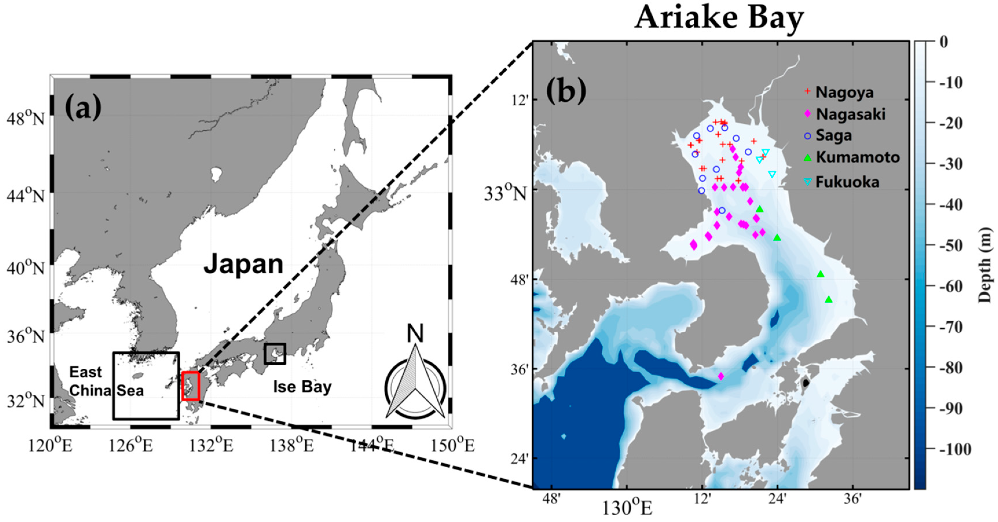
2.1. In Situ Data

The in situ bio-optical and biological data utilized in this study came from three different sources; Nagoya University, Nagasaki University, and the Fisheries Research institutes located around Ariake Bay (Table 1, Figure 1). We also used data from the East China Sea and Ise Bay (Table 1, Figure 1). Datasets from the Nagoya and Nagasaki universities, the East China Sea, and Ise Bay comprise Chl-a, Rrs, and spectral absorption of phytoplankton, non-phytoplankton particles, and CDOM.
In this study, different combinations of datasets (Table 1) were used to achieve our objective. The Nagoya and Nagasaki universities datasets were used for the evaluation of Rrs and development of the in-water algorithm. The two datasets represent the different water characteristics of the Ariake Bay, as the Nagoya University dataset was collected from the northern part of the bay, whereas the Nagasaki University dataset was mostly collected from the southern and inner parts of the bay. Along with these two datasets, the Chl-a datasets from the local Fisheries Research institutes were used to evaluate the standard MODIS Chl-a product and validate the new techniques that we developed. To classify the waters of Ariake Bay into several classes based on the optical properties of its water constituents, the datasets from Nagoya and Nagasaki universities, and those from the East China Sea and Ise Bay datasets were used. The development of the switching algorithm relied on the Nagoya and Nagasaki universities and East China Sea datasets. The East China Sea data, which included low Chl-a concentrations, increased our Chl-a range.

2.1.1. Measurement of Chl-a

Water samples for Chl-a analysis were collected from the sea surface, filtered through 25-mm glass-fiber filters (GF/F) under 0.01 kPa. Chl-a was extracted using N,N-dimethylformamide [23]. Samples collected by the Nagasaki and Nagoya universities in the Ariake Bay, and from the East China Sea and Ise Bay, were measured in a pre-calibrated Turner Designs Fluorometer 10-AU using the method of Welschmeyer [24]. Chl-a concentrations in samples collected by other institutions were measured using the fluorometric method with 90% acetone extraction [25].

2.1.2. Remote Sensing Reflectance (Rrs)

Rrs values in the Ariake and Ise–Mikawa bays were obtained using a hyperspectral radiometer RAMSES (TriOS, Germany) equipped with two radiance (ARC-VIS) sensors and one irradiance (ACC-VIS) sensor. In order to avoid the direct reflectance of the sunlight at the sea surface, the dome-cover method designed by Tanaka et al. [26] was used for one of the radiance sensors. To correct the self-shading error caused by the dome, we used the double dome-cover method by Kobayashi et al. [27]. In this method, two radiometers with different sizes of domes were placed just above the water surface to measure water-leaving radiances, and the influence of the shadows was estimated and subtracted. RAMSES provides hyperspectral water-leaving radiance (Lw(λ)) and downwelling irradiance (Ed(λ)) at wavelengths from 350 nm to 900 nm at 2-nm intervals. Rrs(λ) was calculated as Rrs(λ) = Lw(λ)/Ed(λ), where λ is the wavelength. Rrs at 443 nm, 488 nm, and 547 nm were used for Chl-a algorithm development. Since 443 nm and 547 nm are not included in this sensor, the Rrs at these two wavelengths were obtained by the interpolation of Rrs at two adjacent wavelengths. We also used a set of RAMSES with onboard irradiance, above water radiance, and sky radiance sensors for some of the Nagasaki University datasets. For these datasets, the dome-cover method of Tanaka et al. [26] was adopted. The self-shading error was not corrected for those datasets because we could not evaluate the influence of the self-shading error on the Rrs data with only one size of dome was used. However, when we overlapped those datasets with other in situ datasets in the plot of Chl-a versus R, we found that they overlapped. Accordingly, the influence of self-shading error is probably not much. In some of the clearer waters of Ariake Bay and the East China Sea, we also used an underwater profiling reflectance radiometer (PRR-800) with an onboard irradiance meter, PRR-810 [28]. We assume that the Rrs data estimated from PRR-800/810 and RAMSES are equivalent for this study, although these estimations are not strictly equivalent.

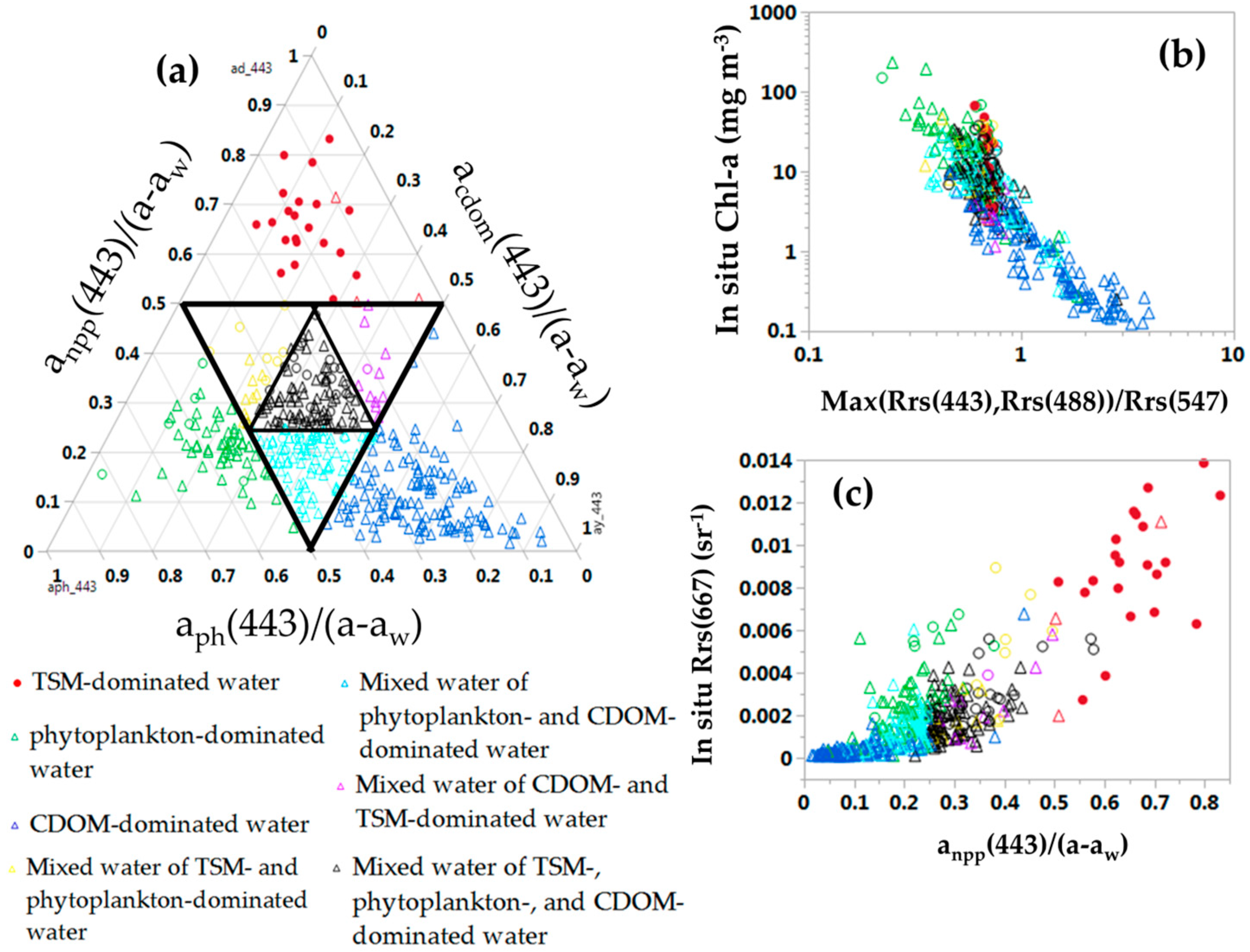
2.1.3. Absorption by CDOM, Phytoplankton, and NPP

For measurements of absorption coefficients (ay(λ)) of CDOM, water samples were filtered sequentially through 47-mm Whatman GF/F and 47-mm of 0.2-µm pore size Nuclepore membrane filters to remove the large and small particles, respectively. The absorbance of the filtered water was measured over the wavelength range of 300–800 nm with 1-nm intervals using a Shimadzu MPS-2400 spectrophotometer with a 10-cm path length quartz cell. Absorbance values were converted to the absorption following the equation [29]:
a y ( λ ) = 2.303 l [ [ OD s ( λ ) OD bs ( λ ) ] OD null ] ,
where l is the path length of the quartz cell, ODs(λ) is the optical density of the filtered water sample, ODbs(λ) is the optical density of purified water, and ODnull(λ) is the apparent residual optical density at a long visible or near infrared wavelength where absorption by dissolved materials is assumed to be zero.
Measurements of the absorption coefficients of phytoplankton (aph(λ)) and NPP (anpp(λ)), and absorption coefficients of total particles (ap(λ)) were undertaken using the filter-pad technique [30]. Water samples were filtered through a 25-mm Whatman GF/F. The filtered volume was decided by visual inspection of the color of the filter. Filters were stored in the liquid nitrogen before measurement of the absorbance of particles using a Shimadzu MPS-2400 spectrophotometer with a scan range of 350–750 nm and 1-nm intervals. This provided an estimate of the absorption by total particles, ap(λ). ap(λ) was calculated from the absorbance after correcting for the path length amplification [31]. Then, all of the pigments on this filter paper were extracted using methanol, and the absorption measured again provided the absorption coefficient of all of the non-phytoplankton particles (anpp(λ)). To derive aph(λ), absorption by only phytoplankton pigments, anpp(λ) was subtracted from ap(λ).

2.1.4. Measurements of Total Suspended Matter

For total suspended matter (TSM), 100 mL or 200 mL of seawater was filtered through prewashed 47-mm Nuclepore membrane filters with 0.2-µm pore size, which were then washed using Milli-Q water, and immediately frozen prior to further processing in the lab where they were dried in the oven at 60 °C. The dried filters were moved to a desiccator and weighed after they reached room temperature. To calculate the concentration of TSM, the average weight of blank filters was subtracted from the weight of the sample filter to derive the weight of TSM, which was then normalized to the volume of filtered water.

2.2. Satellite Data

MODIS reprocessed 2014 L2 data were obtained from the NASA Ocean Biology Processing Group (OBPG) data portal at http://oceancolor.gsfc.nasa.gov. For validation of the satellite data, a maximum time difference of 3 h between in situ sampling and satellite measurements was allowed. The value of the nearest pixel to the location of an in situ station from the 3 × 3 window was used. Data were discarded if they were flagged for LAND, HIGLINT, HILT, HISATZEN, CLDICE, HISOLZEN, LOWLW, MAXAERITER, and NAVFAIL. Descriptions of those flags are illustrated in the following website; https://oceancolor.gsfc.nasa.gov/atbd/ocl2flags/.

2.3. Recalculation of Rrs

The standard MODIS Rrs products often suffer from significant atmospheric correction errors. Atmospheric corrections in coastal waters are challenging, because often, absorptive aerosols are present in the atmosphere [5]. Furthermore, large errors are expected in waters that are turbid [9]. As it is known that Ariake Bay is turbid, especially in the northern region, and sometimes influenced by anthropogenic aerosols [32], we anticipated that MODIS Rrs measurements would be problematic.
In order to improve the atmospherically corrected standard MODIS Rrs, we used the method of Hayashi et al. [14]. This method assumes that the error in MODIS Rrs(547) is negligible, and that Rrs(412) can be estimated based on a linear relationship between in situ Rrs(412) and Rrs(547). The method also assumes that Rrs errors decrease linearly from the blue (412 nm) to green (547 nm) bands. Then, the error in MODIS Rrs at λ between 412 nm and 547 nm was derived based on the error at Rrs(412) using the following relationship:
Error   of   Rrs ( λ ) = Error   of   Rrs ( 412 ) × 547 λ 547 412 ,
This method was developed for a small semi-enclosed bay similar to Ariake Bay. Hayashi et al. [14] suggested that the method is applicable to other areas where there is a linear relationship between Rrs(412) and Rrs(547), although the parameters of the linear relationship could vary with areas.
Hayashi et al. [14] recalculated Rrs(λ) only when MODIS Rrs(412) was less than Rrs(412) estimated from Rrs(547). However, in this study, Rrs(λ) was also recalculated when MODIS Rrs(412) was greater than Rrs(412) estimated from Rrs(547).

2.4. Statistical Analysis

To evaluate the error in retrieved data, the coefficient of determination r2, the slope of retrieved data (Y) on in situ data (X), bias, and root mean square error (RMSE) were used. Bias is a systematic error indicating overestimation or underestimation. RMSE is an indicator of average model performance. The formula of bias and RMSE for Rrs and Chl-a were expressed as [15]:
Relative   Rrs _ Bias ( % ) = 1 N i = 1 N x i × 100 ,
Relative   Rrs _ RMSE ( % ) = 1 N i = 1 N ( x i ) 2 × 100 ,
and:
x = E R r s I R r s I R r s ,
where N is the data number; and ERrs and IRrs represent MODIS and in situ Rrs, respectively.
Log ( Chl - a ) _ Bias = 1 N i = 1 N y i ,
Log ( Chl - a ) _ RMSE = 1 N i = 1 N ( y i ) 2 ,
and:
y = log 10 E C log 10 I C ,
where EC and IC represent estimated and in situ Chl-a, respectively.
We also used absolute relative error:
Absolute _ RE ( % ) = i = 1 N a b s ( E C i I C i I C i ) N × 100 .

3. Results

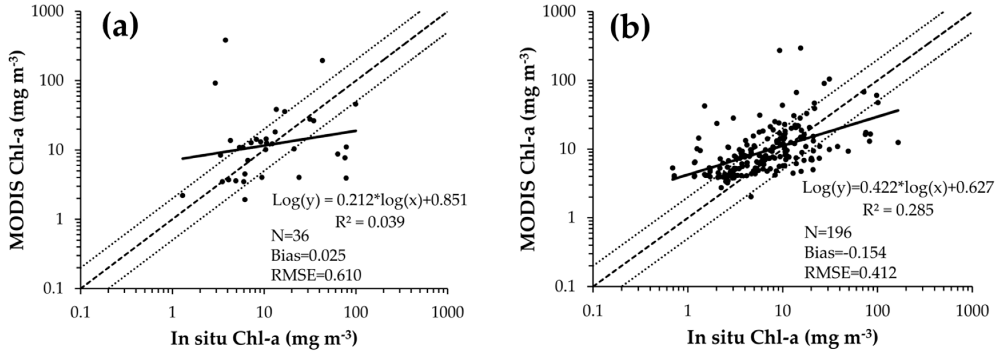
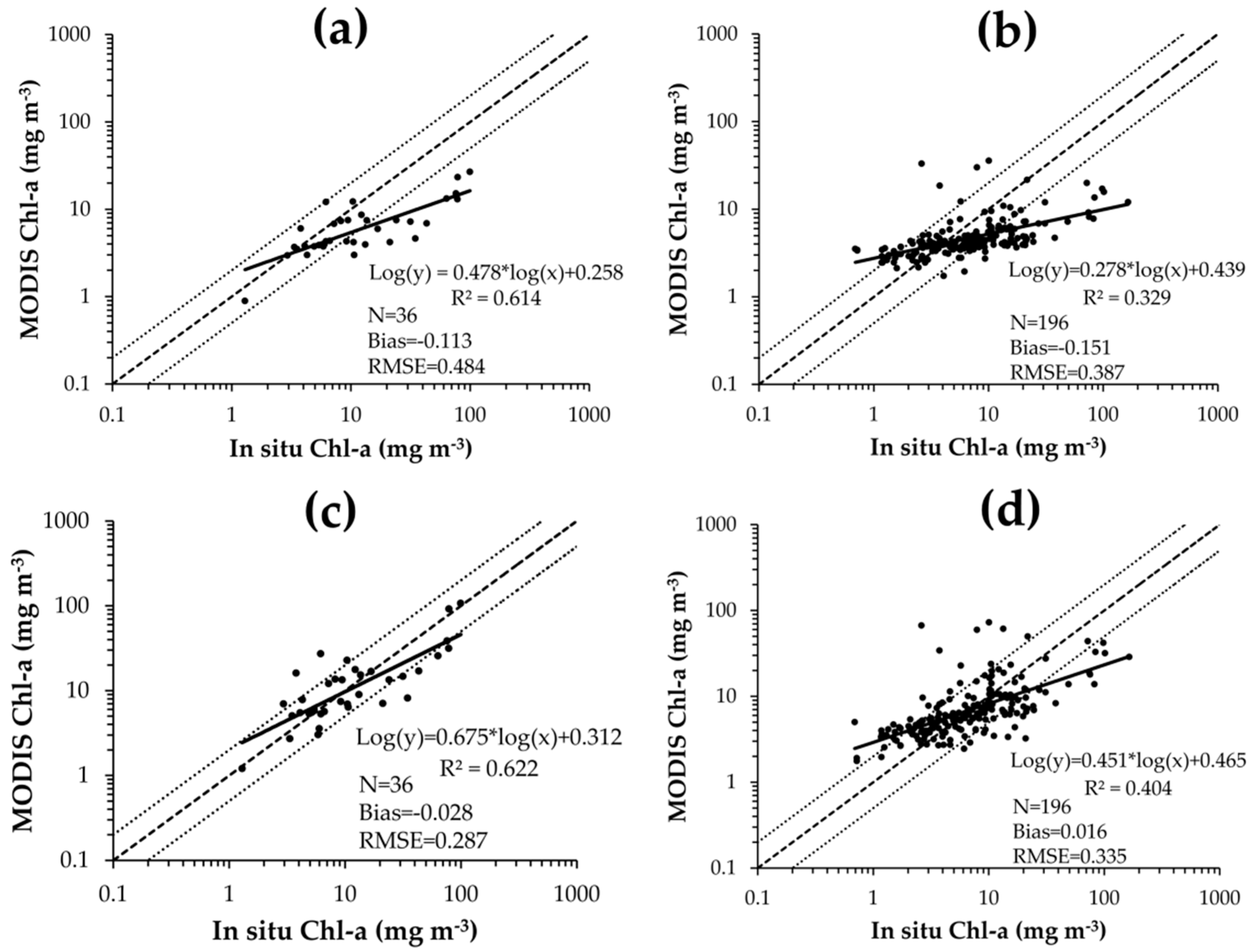
3.1. Evaluation of Standard Satellite Chl-a

Standard MODIS OC3M derived Chl-a was validated using in situ datasets from Nagoya and Nagasaki universities and local Fisheries Research institutes (Table 1). The results showed that the errors in MODIS Chl-a were large (Figure 2). The scatter was large, and some data were either highly overestimated or underestimated (outside of Y = 2X and Y = X/2 lines, respectively). Statistically, the large errors were indicated by the low slopes of the regression line, low r2, large bias, and high RMSE, suggesting the need for improvement in MODIS Chl-a retrievals.

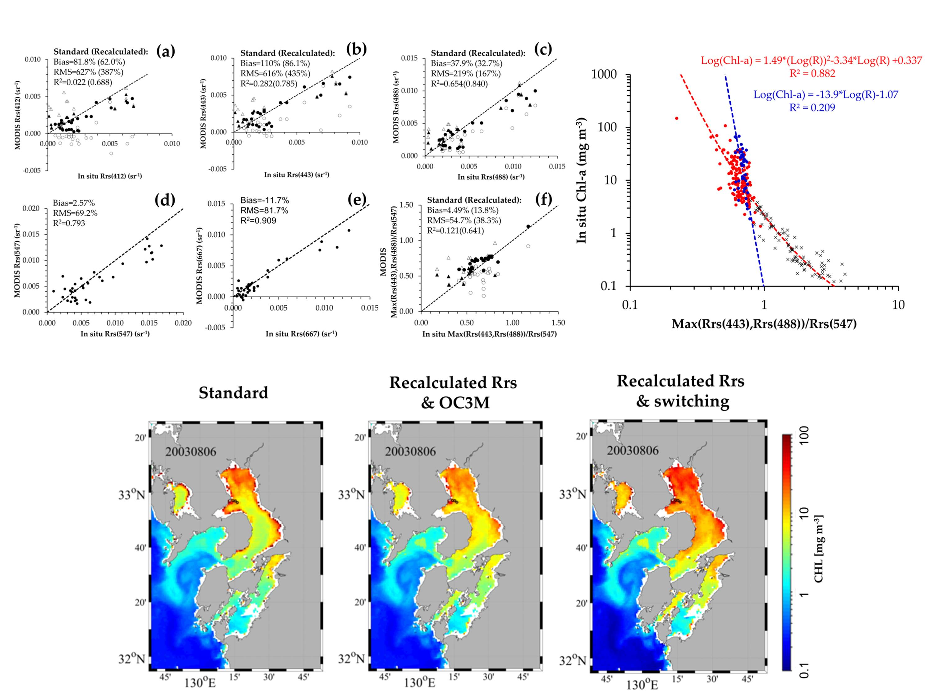
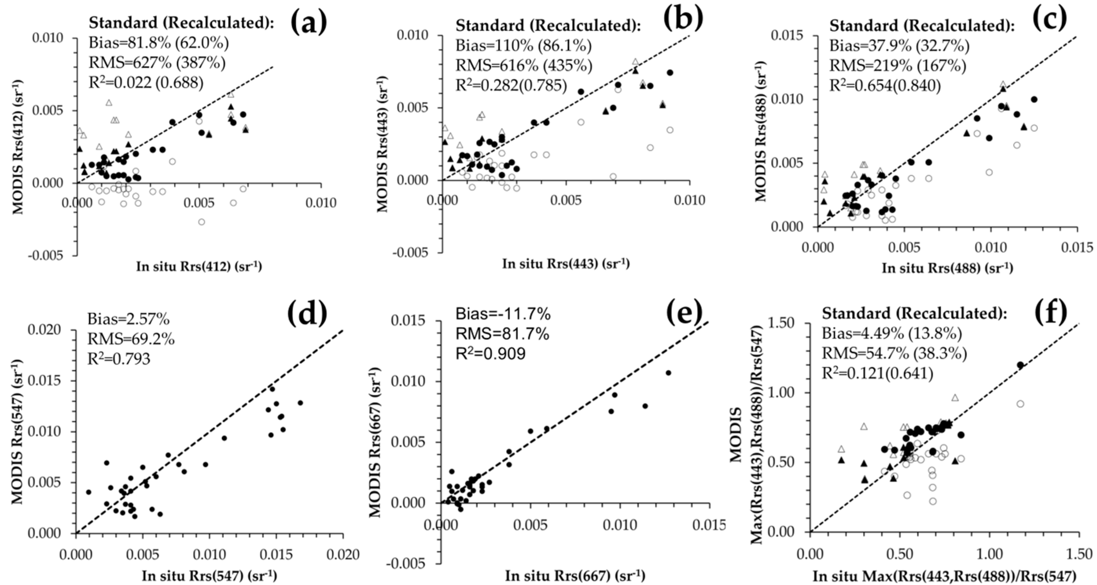
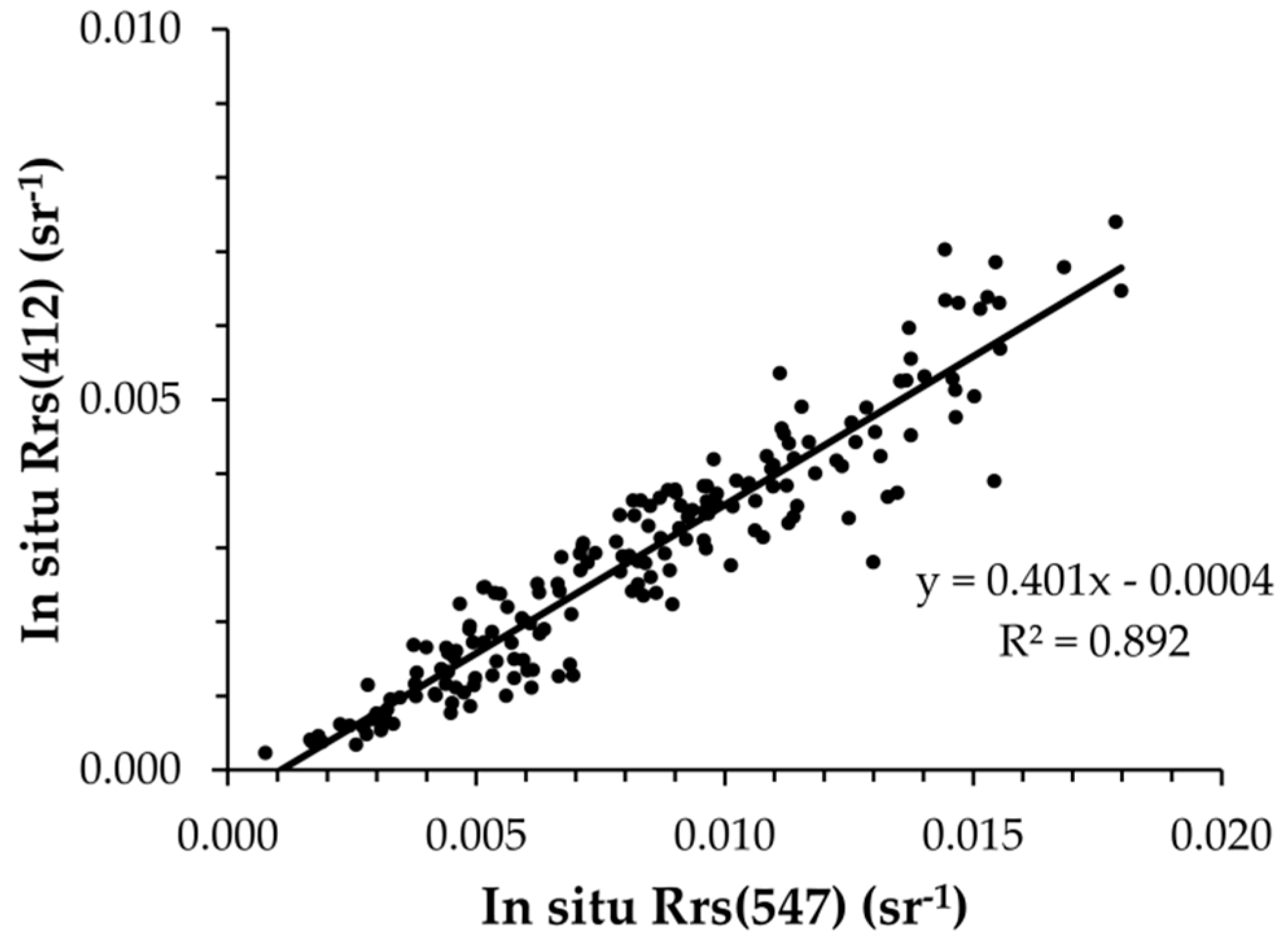
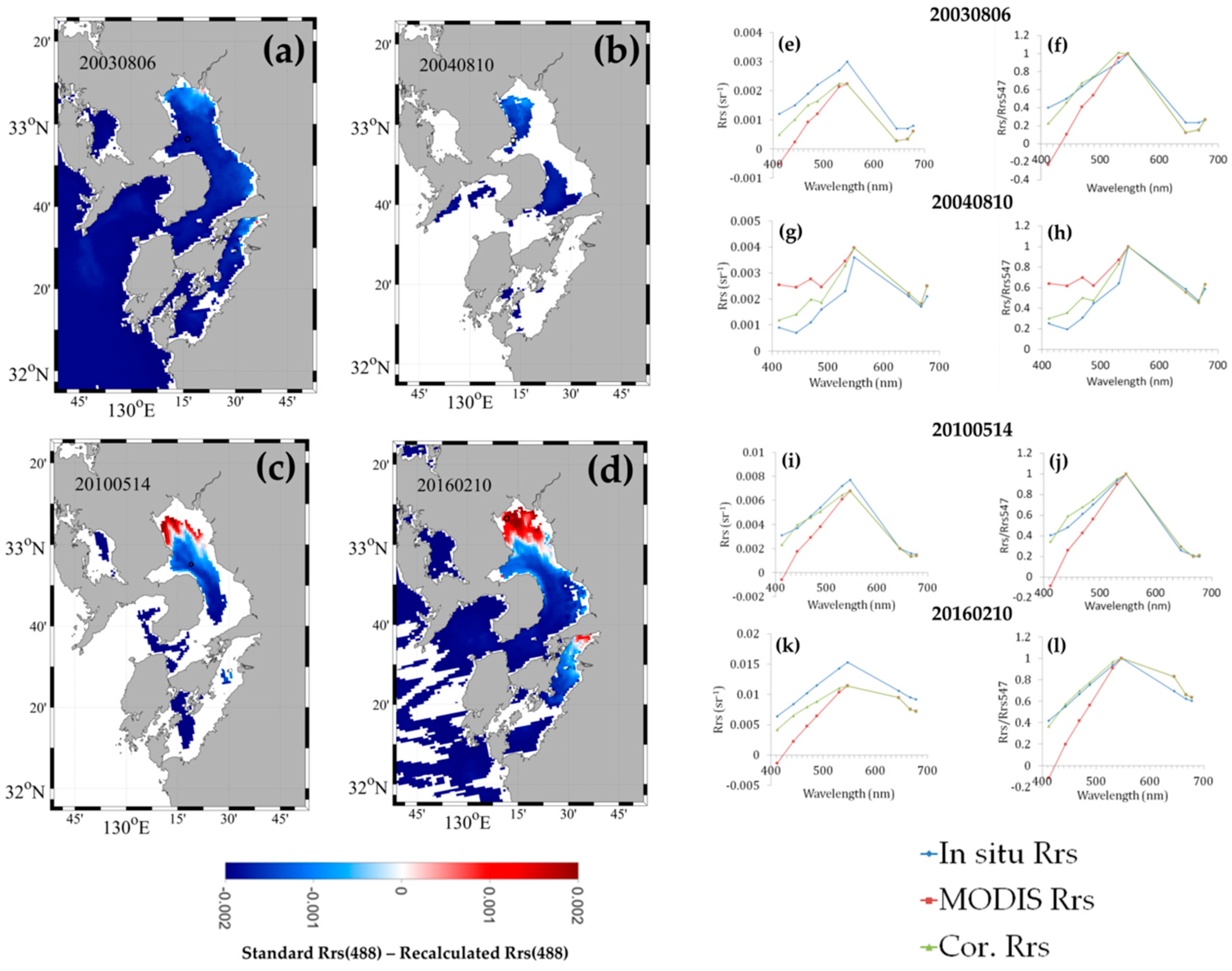
3.2. Validation and Recalculation of Rrs

To examine the sources of the large errors in MODIS Chl-a, we began by investigating errors in MODIS Rrs values (Figure 3). The values at shorter wavelengths, especially at 412 nm, were often negative, and the standard atmospheric correction algorithm was inadequate to provide accurate MODIS Rrs retrievals for Ariake Bay. The correlation between MODIS and in situ Rrs was statistically insignificant (r2 = 0.282, 0.654), and the bias (110%, 37.9%) and RMSE (616%, 219%) were large at 443 nm and 488 nm. In contrast, MODIS Rrs(547) showed a strong correlation (r2 = 0.793) with in situ Rrs(547) and smaller bias (2.57%) and RMSE (69.2%) (Figure 3d). Consequently, the correlation between MODIS and in situ R, for a standard MODIS OC3M algorithm, was also weak (r2 = 0.121), and the bias (4.49%) and RMSE (54.7%) were large. These observations indicate that MODIS Rrs at 443 nm and 488 nm needed to be improved for the accurate retrieval of MODIS Chl-a.
In order to apply the improvement method of Hayashi et al. [14], we had to take into account several assumptions and steps, which are described in Section 2.3. First of all, the error in MODIS Rrs(547) should be small to apply this method. As described above, the error in MODIS Rrs(547) was smaller than the error in Rrs from shorter wavelengths (Figure 3), so MODIS Rrs(547) could be directly used for the improvement of Rrs at shorter wavelengths. Secondly, it should be possible to estimate Rrs(412) from Rrs(547), and the strong correlation between in situ Rrs(412) and Rrs(547) for Ariake Bay data (r2 = 0.892) fulfilled this condition (Figure 4). Furthermore, a comparison of Rrs(547) and Rrs(488) showed Rrs(547) to be mostly larger than Rrs(488) (cf. Figure 4). Thus, this relationship could be used to improve MODIS Rrs(412) from MODIS Rrs(547) in cases when Rrs(547) was greater than Rrs(488).
Thirdly, in order to apply this method, the error in Rrs(λ) should decrease linearly with the wavelengths from 412 nm to 547 nm. For most of the match-up data this assumption held true, although for some match-up cases, the magnitude of errors in Rrs(412) and Rrs(547) was nearly equal. Fourthly, Hayashi et al. [14] only recalculated MODIS Rrs when the standard MODIS Rrs(412) was smaller than the Rrs(412) estimated from the Rrs(547) because they assumed that the error arises mostly from absorptive aerosols. In Ariake Bay, errors may arise not only from absorptive aerosols, but also from the turbidity of water as well as for other reasons, such as the adjacency effect of the coast. After checking the entire match-up dataset, we decided to use this recalculation method also in cases where MODIS Rrs(412) was greater than the estimated values (from the Rrs(412) versus Rrs(547) relationship) because other assumptions were correct.
After recalculation of Rrs, the negative Rrs values at 412 nm and 443 nm disappeared (Figure 3), and the RMSE of these recalculated MODIS Rrs versus in situ data showed a reduction of 38.3%, 29.4%, and 23.7% for Rrs(412), Rrs(443), and Rrs(488), respectively (Figure 3). Bias in Rrs(412), Rrs(443), and Rrs(488) also decreased by 24.2%, 21.7%, and 13.7%, respectively. The improvement in Rrs data also resulted in an improvement of the RMSE of R by 30.0%, although the bias of the ratio increased slightly. Thus, it is clear that the recalculation method of Hayashi et al. [14] effectively improved the MODIS Rrs and Rrs band ratio, and consequently Chl-a retrievals.
MODIS Rrs(488) was either underestimated or overestimated when compared to the recalculated Rrs(488) (Figure 5). We compared Rrs(488) because Rrs(488) is mostly used in the OC3M algorithm and our switching algorithm, which will be described later. MODIS Rrs(488) was lower than the recalculated Rrs(488) for the whole study area on 14 May 2010. In contrast, Rrs(488) was lower near the coast and higher in the middle bay on 6 August 2003 and 10 February 2016. The spectra from the match-up points indicate that the error in recalculated Rrs arose from an underestimation of MODIS Rrs(547) as well as Rrs(412), as shown in the comparison of Rrs spectra in Figure 5. Despite this, when compared to in situ data, the recalculated Rrs was more accurate than the MODIS Rrs. In addition, the normalized Rrs was also processed for easier comparison among the Rrs spectra. The error in MODIS Rrs may be caused by aerosols, which gives rise to underestimation at short wavelengths and a covered large area of the study area, or by the coastal turbidity, which also gives rise to underestimation at the short wavelengths. From the Rrs spectra corresponding to the four images, only one data showed overestimation of Rrs(547); moreover, the cause of the error was more likely to be stray light. On the other hand, Rrs(488) was higher on 10 August 2004, when a large part of the data was missing because of cloud cover. The Rrs spectra also showed an irregular shape with relatively higher Rrs at the shorter wavelengths and abnormal variation between Rrs(412) and Rrs(547). The NASA flag indicated that the influence of the stray light as well as the large cloud coverage may have caused this irregular shape. It is encouraging that in spite of the above-mentioned discrepancies, in most cases, the error in Rrs(488) and R was reduced using the recalculation method of Hayashi et al. [14].

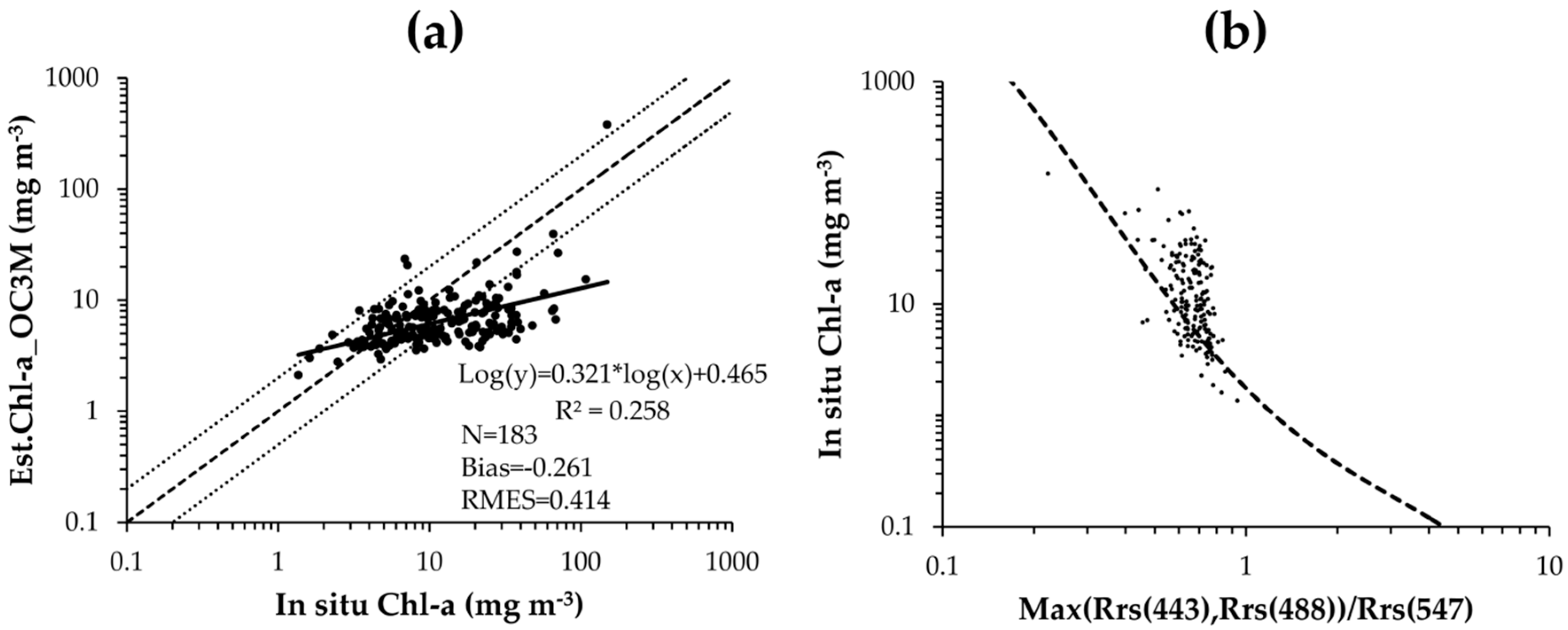
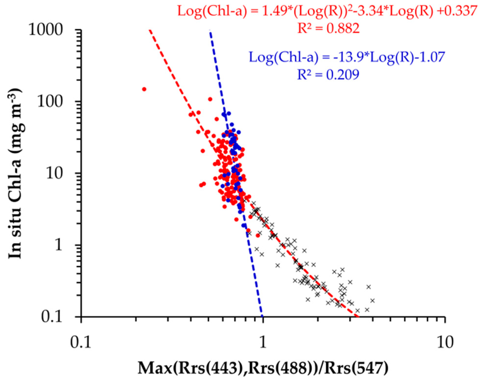
3.3. Validation and Improvement of In-Water Algorithm

To further improve MODIS Chl-a, the MODIS standard in-water algorithm, OC3M [33], was evaluated using in situ Rrs and Chl-a from the datasets of Nagoya and Nagasaki universities (Figure 6a). In the earlier version of the current OC3M algorithm that obtained Chl-a from Rrs, O’Reilly et al. [33] showed that R ranged between 0.1–10. Our current observations in the Ariake Bay showed a narrower range of R between 0.5–0.9 and the absence of low Chl-a values (<1 mg m−3). It is clear that most of the data was significantly underestimated by OC3M (Figure 6a).
The deviations in data from the line of fit between Chl-a and R were examined in relation to in-water constituents of Chl-a, TSM, and CDOM (ay(412)) measured in the Ariake Bay (Table 2). What was immediately apparent was that the average and range of Chl-a, TSM, and CDOM were higher than those encountered in the open ocean. The variations were especially large for Chl-a and TSM. We also examined the relationship of in situ Chl-a, TSM, and CDOM, with the inherent optical properties, aph(443), anpp(443), and ay(443), respectively, and found that they were correlated (r2 = 0.673, 0.027, and 0.991, respectively). Thus, the proportion of each index to the total absorption can be used as the proportion of each water constituent. The mean of the proportions of the absorptions showed that the contributions of anpp(443) (37.5%) and aph(443) (36.0%) were larger than the contribution of ay(443) (26.5%); however, the proportions were essentially very close to each other, indicating that the optical property was of Case 2 water, where phytoplankton is not dominant [34].
In order to understand the relationship between Chl-a and R, the water types of Ariake Bay, the East China Sea, and Ise Bay were separated by the proportions of aph(443), anpp(443), and ay(443), as in Prieur and Sathyendranath [35] (Figure 7a). The analysis separated the data into seven water types. Most of the data from Ariake Bay belonged to the TSM-dominated water type, while a small amount of data belonged to phytoplankton-dominated or mixed water types. Furthermore, the data from the TSM-dominated water type were mostly from Ariake Bay. In addition, the relationship between Chl-a and R in TSM-dominated waters from Ariake Bay showed a higher slope than that from other waters (Figure 7b).
The correspondence of the high TSM water with a high slope for Chl-a versus R (Figure 7b), and the observation that the high TSM was responsible for the underestimation of Chl-a in the northern Ariake Bay, made it possible to develop an algorithm that could be switched between non-turbid and turbid waters. For this study, we relied on same approach as that of Robinson et al. [36], in which Rrs(670) is used as an index of turbidity to separate turbid and non-turbid waters. Based on the strong relationship between Rrs(667) and the proportion of anpp(443) (Figure 7c), we confirmed that Rrs(667) could be used as an indicator of turbidity in Ariake Bay.
As stated earlier, Rrs(667) was used to separate the non-turbid water from turbid water. For non-turbid water, a second order polynomial was fitted to the relationship between log(Chl-a) and log(R), whereas a linear function was fitted to the turbid datasets using type II regression (Figure 8). A threshold was chosen to make the higher r2 and lower RMSE for both regressions. In other words, Rrs(667) ≤ 0.005 and Rrs(667) > 0.005 corresponded to non-turbid and turbid waters, respectively. The fitted algorithms are the following:
Log(Chl-a) = 1.49*(Log(R))2 − 3.34*Log(R) + 0.337,
for non-turbid water and:
Log(Chl-a) = −13.9*Log(R) − 1.07,
for turbid water.
The error of the switching algorithm was smaller than the error of the OC3M algorithm for both non-turbid and turbid waters (Figure 8). The estimated Chl-a was also closer to the in situ data from Ariake Bay, as well as from the subsets, than it was to estimates from OC3M in terms of slope, r2, bias, and RMSE (Table 3).

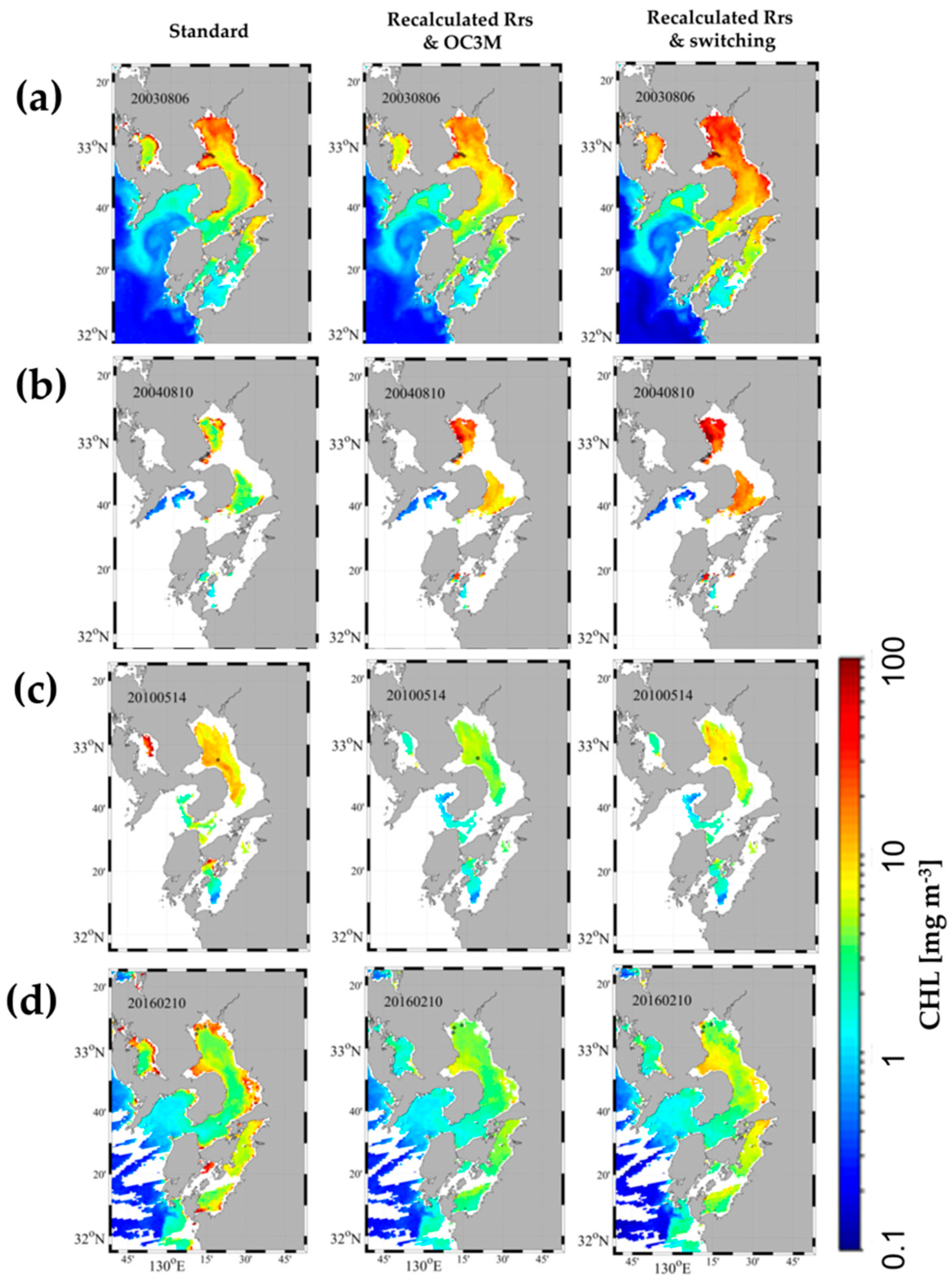
3.4. Evaluation of the Improved MODIS Chl-a

To assess the improvement in MODIS Chl-a retrievals, the recalculation method of Rrs described above was first applied to MODIS Rrs. The improved MODIS Rrs were then used to obtain refined MODIS Chl-a data using the standard OC3M algorithm (Figure 9a,b). After our Rrs recalculation, MODIS Chl-a improved significantly (r2 = 0.614, RMSE = 0.484) compared with the standard Chl-a (r2 = 0.039, RMSE = 0.610; Figure 2a) when compared to the in situ dataset of Nagoya and Nagasaki universities. However, the slopes were still low (0.478; Figure 9a), and some data were either greatly underestimated or overestimated. In order to further improve MODIS Chl-a, our switching algorithm was then used, and the new MODIS Chl-a values showed not only an improved slope (0.675) and bias (−0.028), but also a higher r2 (0.622) and a lower RMSE (0.287) (Figure 9c). Besides, the scatter in the data was also greatly reduced, and most of the data were within a factor of 2 and 1/2 of the in situ data.
The improvement in MODIS Chl-a was further validated by the independent dataset collected by the Fisheries Research institutes from not only the inner parts of the bay, but also the southern region. Using the OC3M algorithm and the recalculated Rrs, the Chl-a retrievals improved considerably (r2 = 0.329, RMSE = 0.387; Figure 9b) compared to retrievals using MODIS Rrs (r2 = 0.285, RMSE = 0.412; Figure 2b). Additionally, when the OC3M algorithm was replaced by the new switching algorithm, the estimated MODIS Chl-a improved further (r2 = 0.404, RMSE = 0.335; Figure 9d).
In addition to the validation of MODIS Chl-a using in situ data, new MODIS Chl-a images were generated using the recalculated MODIS Rrs and the standard and switching algorithms (Figure 10). The turbid-water algorithm was applied only for the water where Rrs(667) > 0.005 and in the range of −0.095 > log(R) > −0.223, because our algorithm development and verification dataset covered only this range of log(R). The MODIS Chl-a images indicated that the standard MODIS Chl-a values were high in coastal areas with some values even over 100 mg m−3, but decreased in the middle of the bay and reduced even further offshore. Using the recalculated Rrs, the Chl-a with OC3M showed that the very high Chl-a disappeared, and the change of Chl-a mostly happened in the coastal areas rather than the offshore areas. A comparison of satellite-derived Chl-a using OC3M and the switching algorithm showed that Chl-a derived using the latter algorithm were higher. This is consistent with the underestimation by OC3M that we describe in Section 3.3 (cf. Figure 5). The difference between standard and improved MODIS Chl-a were shown in the supplementary materials (Figure S1).

4. Discussion

4.1. Improvement of Chl-a

Our study revealed the large error in the standard MODIS Chl-a product as demonstrated by the significant negative or positive deviations when compared with in situ Chl-a (Figure 2). The desired absolute error for ocean color Chl-a by NASA is 35% for coastal waters [37,38]. In this section, we discuss the improvement of MODIS Chl-a with respect to the absolute error using recalculated Rrs and our switching algorithm.
When compared to the in situ Chl-a dataset collected by Nagasaki and Nagoya universities, the standard NASA MODIS Chl-a yielded an absolute relative error of 51.7%, which was much larger than the desired value. Our study showed that the major sources of error in the retrievals of Chl-a from MODIS were; (1) the inaccuracy of the standard atmospheric correction [5,10] and (2) the shortcoming of the standard OC3M in the water algorithm for deriving Chl-a [33].
To overcome these shortcomings in the usage of MODIS Chl-a, we utilized all of the available in situ Rrs values from the Nagasaki and Nagoya universities dataset and the approach by Hayashi et al. [14] to first reduce the errors associated with MODIS Rrs. This recalculation helped reduce the absolute error in MODIS Chl-a to within 30.1%. To account for the errors associated with the standard OC3M algorithm especially in the turbid waters at the head of Ariake Bay, a switching algorithm was developed. Using this algorithm reduced the absolute error of the Chl-a to 24.9%. When compared to the match-up dataset, the error in MODIS Chl-a was reduced, and the accuracy was improved above the desired value. Thus, a simple and effective approach that combines the Rrs recalculation method with a locally tuned switching algorithm allowed much more accurate retrievals of satellite Chl-a from this turbid and semi-enclosed bay.
When using the independent and larger Chl-a validation datasets of the Fisheries Research institutes, which covered a wider area of Ariake Bay was compared to the standard MODIS Chl-a, the absolute relative error was 84.0%. After improving the Rrs using the recalculation method of Hayashi et al. [14], the error in Chl-a retrievals was reduced to 57.3%. However, when using our switching algorithm, the error in Chl-a retrievals increased slightly by 1.1%, although various statistical tests showed improved Chl-a estimations. Considering that our optical data was limited for such a complex optical system, this is a satisfactory improvement, even though we did not attain the accuracy in Chl-a retrievals that is recommended by NASA. Further discussion of the atmospheric correction and in-water algorithm follow.

4.2. Atmospheric Correction

To investigate the spatial distribution of MODIS Rrs error, we processed satellite images to obtain the difference between the standard and recalculated MODIS Rrs(488). The images showed that the error in the coastal areas was negative, suggesting that this underestimation of MODIS Rrs could be caused by turbidity, which is high in those areas (Table 2). It is expected that the turbidity of Ariake Bay contributed to the error in MODIS Rrs. Turbidity is one of the important causes for the failure of the atmospheric correction algorithm because the black pixel assumption breaks down in turbid waters [6]. Specifically, the radiance of the atmosphere in the bands shorter than the near-infrared region is often overcorrected because of the near-infrared reflectance from the ocean; thus, the Rrs will be underestimated, especially at shorter wavelengths [6,39]. Negative values of Rrs(412) and Rrs(443) were consistently encountered in MODIS data, especially at locations closer to the head of Ariake Bay, reinforcing the idea that the effectiveness of atmospheric correction algorithms in turbid waters is limited.
In addition, the image showing the difference between the standard and recalculated MODIS Rrs(488) for 14 May 2010 showed an underestimation of Rrs for the whole Ariake Bay. This indicates that there was another possible cause for the underestimation of Rrs in this area. It has been suggested that Kosa (Yellow Sand Dust) and other aerosols influence the western part of Japan, including Ariake Bay [32,40,41,42]. The larger underestimation was probably related to one of the atmospheric events. Large improvements in Rrs retrievals by the Hayashi et al. [14] method showed the effectiveness of this method in mitigating the shortcomings of current standard atmospheric correction. What makes the recalculation method of Hayashi et al. [14] particularly attractive is that it is simple; it requires no a priori information of the aerosols, and no tweaking of the standard atmospheric correction models for local use. Even if prior information is available on the type and quantity of absorbing aerosols, parameterizing atmospheric correction models and running these models is computationally intensive and particularly challenging given the highly dynamic nature of atmospheric aerosols.
For the recalculation method of Hayashi et al. [14], the linear relationship between in situ Rrs(412) and Rrs(547) was used to recalculate Rrs(412). They observed the relationship in Ise–Mikawa Bay where is another semi-enclosed bay in Japan [14]. The linear relationship was also observed in Ariake Bay, although the slope of the relationship was different from the Ise–Mikawa Bay. In our study, we found that the correlation was strong for the data under the condition that Rrs(488) was less than Rrs(547), which indicated that the water was not very clear. We expect the relationship between in situ Rrs(412) and Rrs(547) in other similar optical waters.
Hayashi et al. [14] found that an overestimation of MODIS Chl-a coincided with negative MODIS Rrs(412), which was to be expected because of absorptive aerosols. This led them to use the Rrs recalculation method, which reduced the MODIS Rrs underestimation. In Ariake Bay, we found not only underestimation, but also an overestimation of Rrs(412), both of which produce errors in Chl-a. One cause for the overestimation of Rrs could be stray light. However, it is more likely that errors were caused by the wrong atmospheric model selection, especially in turbid waters, and for a small semi-enclosed sea [43]. In this study, we applied the method not only for underestimations, but also overestimations of MODIS Rrs, and our results show that Rrs improved in both cases (Figure 3). This study thus shows that the simple method of Hayashi et al. [14] is of great utility to improve the underestimation of Rrs caused by absorptive aerosols and high turbidity as well as the overestimation of Rrs, the reasons of which are unclear to us.
It is worth mentioning two other factors that cause the error of the Rrs. One is the “adjacency effect”, which is defined as the spatial mixing of radiance among nearby pixels [44]. Since Ariake Bay is a relatively small semi-enclosed bay, the reflectance from the coast is likely to affect the reflectance from the waters. The other one is the degradation of MODIS, especially for the shorter wavelength [45]. Lee et al. [45] revealed that the degradation already started from 2005, and the calibration bias could be up to 1.8% at 412 nm.

4.3. In-Water Algorithm

Satellite Chl-a retrievals from the Ariake Bay using the standard OC3M in-water algorithm severely underestimated Chl-a comparing to in situ data, especially when Chl-a was over 10 mg m−3 (Figure 6). It is well-known that the empirical OC3M algorithm was developed using data mostly from the open ocean, and hence OC3M is not suitable for coastal waters. In addition, OC3M uses R, and was developed for Case 1 waters, in which water constituents are dominated by phytoplankton and their associated materials [34,46]. However, in coastal waters, CDOM and NPP, which absorb and scatter light, do not co-vary with phytoplankton, resulting in an overestimation of Chl-a [47,48]. Our validation of OC3M in Ariake Bay showed that the OC3M algorithm often underestimates Chl-a. Therefore, our regional algorithm for Ariake Bay is of great utility for both researchers and resource managers.
The water constituents of Ariake Bay were analyzed using the ternary diagram similar to that in Prieur and Sathyendranath [35] before we developed the regional algorithm, and we found that underestimates by OC3M were mostly from anpp-dominated and TSM-dominated waters. We also know that the waters in the southern part of the bay and outside of the bay were less turbid. Therefore, we separated the data into two groups based on the turbidity of the water using Rrs(667) as criteria. For each group, we developed a separate empirical algorithm based on R.
Rrs is relatively higher in turbid waters, and the different slope from the relationship of Chl-a to R is probably caused by the high scattering of the light by NPP at the shorter wavelengths, although we do not have light scattering data to substantiate this hypothesis. Our switching algorithm for non-turbid water showed a good correlation; however, for turbid water, the error is still large. Chl-a estimated from the R will be inaccurate, because TSM absorbs and scatters light in blue and green bands [49]. To avoid the influence of TSM, we tried a red-to-green band ratio such as Rrs(678)/Rrs(547) or Rrs(678)/Rrs(488) to estimate Chl-a for turbid waters [18]. However, the estimation by red-to-green band ratio was worse than the estimation from our switching algorithm. Therefore, we decided to use the blue-to-green band ratio in the turbid water algorithm.

5. Conclusions

Our results showed that a combination of the simple Rrs recalculation method and the switching algorithm for both non-turbid and turbid waters effectively reduces the error in Chl-a that arises when the standard OC3M is used in the turbid and semi-enclosed Ariake Bay. The improvement in Chl-a values that is obtained through this approach offers the potential for its use in other coastal ecosystems plagued by similar problems. Our Rrs recalculation method is much simpler and computationally less intensive than a complex alternative atmospheric correction. Therefore, we recommend the application of this Rrs recalculation method to deal with the atmospheric correction problems in other similar regions.
Our results also showed that the in-water algorithm could be improved by separating the complex coastal waters into different water types before fitting the data using Chl-a against the blue-to-green band ratio (R). The failure of the standard OC3M algorithm in Ariake Bay was mainly due to turbidity of the water; therefore, we separated the data into non-turbid and turbid water. For non-turbid water, the correlation between Chl-a and R was significant; however, the correlation for turbid water was not statistically significantly. So, it is necessary that we continue to work on improving the Chl-a algorithm for turbid water.

Supplementary Materials

The followings are available online at https://www.mdpi.com/2072-4292/10/9/1335/s1, Figure S1: Difference between standard MODIS Chl-a and corrected Chl-a by OC3M or switching algorithm.

Author Contributions

M.M.Y. and J.I. conceived and performed the research plan and analysis; M.M.Y. and E.d.R.M. processed the data and produced the satellite images; T.K. and N.F. helped in situ data collection; K.S., T.M. and H.Y. provided validation data; A.M. supported statistical analysis; M.M.Y. wrote the paper; J.I., J.I.G., H.d.R.G., E.d.R.M., T.K. and M.H. revised the paper.

Funding

This research was financially supported by Fisheries Agency of Japan and by GCOM-C project of the Japan Aerospace Exploration Agency.

Acknowledgments

We thank member of Institute for Lowland Technology, Saga University for their support to use their laboratory. We also thank Saga Ariake Fisheries Promotion Center, Kumamoto Prefectural Fisheries Research Center and Fukuoka Fisheries and Marine Technology Research Center, for their supply of in situ data. We also thank Salem Ibrahim Salem, a postdoctoral fellow from Oki Laboratory, the Institute of Industrial Science, University of Tokyo, Japan, for his editing of the paper. At last, we thank the NASA Goddard Space Flight Center, the Ocean Ecology Laboratory and Ocean Biology Processing Group for providing the Moderate-resolution Imaging Spectroradiometer (MODIS) Aqua L2 data.

Conflicts of Interest

The authors declare no conflict of interest.

References

  1. Shin, M.; Lee, H.J.; Kim, M.S.; Park, N.B.; Lee, C. Control of the red tide dinoflagellate Cochlodinium polykrikoides by ozone in seawater. Water Res. 2017, 109, 237–244. [Google Scholar] [CrossRef] [PubMed]
  2. Tsutsumi, H. Critical events in the Ariake Bay ecosystem: Clam population collapse, red tides, and hypoxic bottom water. Plankton Benthos Res. 2006, 1, 3–25. [Google Scholar] [CrossRef] [Green Version]
  3. Suzuki, K.W.; Nakayama, K.; Tanaka, M. Horizontal distribution and population dynamics of the dominant mysid Hyperacanthomysis longirostris along a temperate macrotidal estuary (Chikugo River estuary, Japan). Estuar. Coast. Shelf Sci. 2009, 83, 516–528. [Google Scholar] [CrossRef] [Green Version]
  4. Ishizaka, J.; Kitaura, Y.; Touke, Y.; Sasaki, H.; Tanaka, A.; Murakami, H.; Suzuki, T.; Matsuoka, K.; Nakata, H. Satellite detection of red tide in Ariake Sound, 1998–2001. J. Oceanogr. 2006, 62, 37–45. [Google Scholar] [CrossRef]
  5. Gordon, H.R. Atmospheric correction of ocean color imagery in the Earth Observing System era. J. Geophys. Res. 1997, 102, 17081–17106. [Google Scholar] [CrossRef] [Green Version]
  6. Siegel, D.A.; Wang, M.; Maritorena, S.; Robinson, W. Atmospheric correction of satellite ocean-color imagery: The black pixel assumption. Appl. Opt. 2000, 39, 3582–3591. [Google Scholar] [CrossRef] [PubMed]
  7. Goyens, C.; Jamet, C.; Schroeder, T. Evaluation of four atmospheric correction algorithms for MODIS images over contrasted coastal waters. Remote Sens. Environ. 2013, 131, 63–75. [Google Scholar] [CrossRef]
  8. Shehhi, M.R.; Gherboudj, I.; Zhao, J.; Ghedira, H. Improved atmospheric correction and chlorophyll-a remote sensing models for turbid waters in a dusty environment. ISPRS J. Photogramm. Remote Sens. 2017, 133, 46–60. [Google Scholar] [CrossRef]
  9. Wang, M.; Shi, W. The NIR-SWIR combined atmospheric correction approach for MODIS ocean color data processing. Opt. Express 2007, 15, 15722–15733. [Google Scholar] [CrossRef] [PubMed]
  10. Wang, M.; Son, S.; Shi, W. Evaluation of MODIS SWIR and NIR-SWIR Atmospheric correction algorithm using SeaBASS data. Remote Sens. Environ. 2009, 113, 635–644. [Google Scholar] [CrossRef]
  11. Schroeder, T.; Behnert, I.; Schaale, M.; Fischer, J.; Doerffer, R. Atmospheric correction algorithm for MERIS above case-2 waters. Int. J. Remote Sens. 2007, 28, 1469–1486. [Google Scholar] [CrossRef]
  12. Brajard, J.; Santer, R.; Crépon, M.; Thiria, S. Atmospheric correction of MERIS data for case-2 waters using a neuro-variational inversion. Remote Sens. Environ. 2012, 126, 51–61. [Google Scholar] [CrossRef]
  13. Loisel, H.; Vantrepotte, V.; Jamet, C.; Dinh, D.N. Challenges and new advances in ocean color remote sensing of coastal waters. In Topics in Oceanography; Zambianchi, E., Ed.; IntechOpen, 2013; Available online: https://www.intechopen.com/books/topics-in-oceanography/challenges-and-new-advances-in-ocean-color-remote-sensing-of-coastal-waters (accessed on 21 August 2018). [CrossRef]
  14. Hayashi, M.; Ishizaka, J.; Kobayashi, H.; Toratani, M.; Nakamura, T.; Nakashima, Y.; Yamada, S. Evaluation and Improvement of MODIS and SeaWiFS-derived Chlorophyll a Concentration in Ise-Mikawa Bay. J. Remote Sens. Soc. Jpn. 2015, 35, 245–259, (In Japanese with English Abstract). [Google Scholar]
  15. Darecki, M.; Stramski, D. An evaluation of MODIS and SeaWiFS bio-optical algorithms in the Baltic Sea. Remote Sens. Environ. 2004, 89, 326–350. [Google Scholar] [CrossRef]
  16. Dall’Olmo, G.; Gitelson, A.A.; Rundquist, D.C.; Leavitt, B.; Barrow, T.; Holz, J.C. Assessing the potential of SeaWiFS and MODIS for estimating chlorophyll concentration in turbid productive waters using red and near-infrared bands. Remote Sens. Environ. 2005, 96, 176–187. [Google Scholar] [CrossRef]
  17. Gitelson, A.A.; Schalles, J.F.; Hladik, C.M. Remote chlorophyll-a retrieval in turbid, productive estuaries: Chesapeake Bay case study. Remote Sens. Environ. 2007, 109, 464–472. [Google Scholar] [CrossRef]
  18. Le, C.; Hu, C.; Cannizzaro, J.; Duan, H. Long-term distribution patterns of remotely sensed water quality parameters in Chesapeake Bay. Estuar. Coast. Shelf Sci. 2013, 128, 93–103. [Google Scholar] [CrossRef]
  19. Carder, K.L.; Chen, F.R.; Cannizzaro, J.P.; Campbell, J.W.; Mitchell, B.G. Performance of the MODIS semi-analytical ocean color algorithm for chlorophyll-a. Adv. Space Res. 2004, 33, 1152–1159. [Google Scholar] [CrossRef]
  20. Siswanto, E.; Tang, J.; Yamaguchi, H.; Ahn, Y.H.; Ishizaka, J.; Yoo, S.; Kim, S.W.; Kiyomoto, Y.; Yamada, K.; Chiang, C.; et al. Empirical ocean-color algorithms to retrieve chlorophyll-a, total suspended matter, and colored dissolved organic matter absorption coefficient in the Yellow and East China Seas. J. Oceanogr. 2011, 67, 627–650. [Google Scholar] [CrossRef]
  21. Tassan, S. Local algorithms using SeaWiFS data for the retrieval of phytoplankton, pigments, suspended sediment, and yellow substance in coastal waters. Appl. Opt. 1994, 33, 2369–2378. [Google Scholar] [CrossRef] [PubMed]
  22. Yamaguchi, H.; Ishizaka, J.; Siswanto, E.; Son, Y.B.; Yoo, S.; Kiyomoto, Y. Seasonal and spring interannual variations in satellite observed chlorophyll-a in the Yellow and East China Seas: New datasets with reduced interference from high concentration of resuspended sediment. Cont. Shelf Res. 2013, 59, 1–9. [Google Scholar] [CrossRef] [Green Version]
  23. Suzuki, R.; Ishimaru, T. An improved method for the determination of phytoplankton chlorophyll using N,N-dimethylformamide. J. Oceanogr. Soc. Jpn. 1990, 46, 190–194. [Google Scholar] [CrossRef]
  24. Welschmeyer, N. Fluorometric analysis of chlorophyll a in the presence of chlorophyll b and pheopigments. Limnol. Oceanogr. 1994, 38, 1985–1992. [Google Scholar] [CrossRef]
  25. Holm-Hansen, O.; Lorenzen, C.J.; Holmes, R.W.; Strickland, J.D.H. Fluorometric determination of chlorophyll. J. Cons. Perm. Int. Explor. Mer. 1965, 30, 3–15. [Google Scholar] [CrossRef]
  26. Tanaka, A.; Sasaki, H.; Ishizaka, J. Alternative measuring method for water leaving radiance using a radiance sensor with a domed cover. Opt. Express 2006, 14, 3099–3105. [Google Scholar] [CrossRef] [PubMed]
  27. Kobayashi, H.; Ishizaka, J.; Jintasaerance, P.; Gunbua, V.; Fukasawa, T. Water-Leaving Radiance Measured Using with Covered Radiometers in Highly Turbid Waters. In Proceedings of the Ocean Optics XX, Anchorage, AK, USA, 27 September–1 October 2010. [Google Scholar]
  28. Sasaki, H.; Tanaka, A.; Iwataki, M.; Touke, Y.; Siswanto, E.; Tang, C.K.; Ishizaka, J. Optical Properties of Red Tide in Isahaya Bay, Southwestern Japan: Influence of chlorophyll a concentration. J. Oceanogr. 2008, 64, 511–523. [Google Scholar] [CrossRef]
  29. Mitchell, B.G.; Kahru, M.; Wieland, J.; Stramska, M. Determination of spectral absorption coefficients of particles, dissolved material and phytoplankton for discrete water samples. In Ocean Optics Protocols for Satellite Ocean Color Sensor Validation; Mueller, J.L., Fargion, G.S., Eds.; Revision 3; NASA Technical Memorandum: Cleveland, OH, USA, 2002; Volume 2, pp. 231–257. [Google Scholar]
  30. Kishino, M.; Takahashi, M.; Okami, N.; Ichimura, S. Estimation of the spectral absorption coefficients of phytoplankton in a thermally stratified sea. Bull. Mar. Sci. 1985, 37, 634–642. [Google Scholar]
  31. Cleveland, J.S.; Weidemann, A.D. Quantifying absorption by aquatic particles: A multiple scattering correction for glass-fiber filters. Limnol. Oceanogr. 1993, 38, 1321–1327. [Google Scholar] [CrossRef] [Green Version]
  32. Kanayama, S.; Yabuki, S.; Yanagisawa, F.; Motoyama, R. The chemical and strontium isotope composition of atmospheric aerosols over Japan: The contribution of long range-transported Asian dust (Kosa). Atmos. Environ. 2002, 36, 5159–5175. [Google Scholar] [CrossRef]
  33. O’Reilly, J.E.; Maritorena, S.; Siegel, D.A.; O’Brien, M.C.; Toole, D.; Mitchell, B.G.; Kahru, M.; Chavez, F.P.; Strutton, P.; Cota, G.F.; et al. Ocean color chlorophyll a algorithms for SeaWiFS, OC2, and OC4: Version 4. In SeaWiFS Postlaunch Calibration and Validation Analyses: Part 3; Hooker, S.B., Firestone, E.R., Eds.; NASA Technical Memorandum: Cleveland, OH, USA, 2000; Volume 11, pp. 9–23. [Google Scholar]
  34. Morel, A.; Prieur, L. Analysis of variations in ocean color. Limnol. Oceanogr. 1977, 22, 709–722. [Google Scholar] [CrossRef]
  35. Prieur, L.; Sathyendranath, S. An optical classification of coastal and oceanic waters based on the specific absorption curves of phytoplankton pigments, dissolved organic matter, and other particulate materials. Limnol. Oceanogr. 1981, 26, 671–689. [Google Scholar] [CrossRef]
  36. Robinson, W.D.; Franz, B.A.; Patt, F.S.; Bailey, S.W.; Werdell, P.J. Masks and flags updates. In SeaWiFS Postlaunch Technical Report Series; NASA Technical Memorandum: Cleveland, OH, USA, 2003; pp. 34–40. [Google Scholar]
  37. McClain, C.R.; Feldman, G.C.; Hooker, S.B.; Bontempi, P. Satellite data for ocean biology, biogeochemistry, and climate research. EOS 2006, 87, 337–343. [Google Scholar]
  38. Moore, T.S.; Campbell, J.W.; Dowell, M.D. A class-based approach to characterizing and mapping the uncertainty of the MODIS ocean chlorophyll product. Remote Sens. Environ. 2009, 113, 2424–2430. [Google Scholar] [CrossRef]
  39. Wang, M.; Shi, W. Estimation of ocean contribution at the MODIS near infrared wavelengths along the east coast of the U.S.: Two case studies. Geophys. Res. Lett. 2005, 32, L13606. [Google Scholar] [CrossRef]
  40. Li, L.-P.; Fukushima, H.; Frouin, R.; Mitchell, B.G.; He, M.-X.; Uno, I.; Takamura, T.; Ohta, S. Influence of submicron absorptive aerosol on SeaWiFS-derived marine reflectance during ACE-Asia. J. Geophys. Res. 2003, 108. [Google Scholar] [CrossRef]
  41. Toratani, M.; Fukushima, H.; Murakami, H.; Tanaka, A. Atmospheric correction scheme for GLI with absorptive aerosol correction. J. Oceanogr. 2007, 63, 525–532. [Google Scholar] [CrossRef]
  42. Moreno, T.; Kojima, T.; Amato, F.; Lucarelli, F.; de la Rosa, J.; Calzolai, G.; Nava, S.; Chiari, M.; Alastuey, A.; Querol, X.; et al. Daily and hourly chemical impact of springtime transboundary aerosols on Japanese air quality. Atmos. Chem. Phys. 2013, 13, 1411–1424. [Google Scholar] [CrossRef] [Green Version]
  43. Wang, M.; Gordon, H.R. A simple, moderately accurate, atmospheric correction algorithm for SeaWiFS. Remote Sens. Environ. 1994, 50, 231–239. [Google Scholar] [CrossRef]
  44. Adler-Golden, S.M.; Matthew, M.W.; Bernstein, L.S.; Levine, R.Y.; Berk, A.; Richtsmeier, S.C.; Acharya, P.K.; Anderson, G.P.; Felde, G.; Gardner, J.; et al. Atmospheric Correction for Short-Wave Spectral Imagery Based on MODTRAN4. In SPIE Proceedings, Imaging Spectrom; International Society for Optics and Photonics: Denver, CO, USA, 1999; Volume 3753, pp. 61–69. [Google Scholar]
  45. Lee, S.; Meister, G. MODIS Aqua Optical Throughput Degradation Impact on Relative Spectral Response and Calibration of Ocean Color Products. IEEE Trans. Geosci. Remote Sens. 2017, 55, 5214–5219. [Google Scholar] [CrossRef]
  46. Morel, A. Optical modeling of the upper ocean in relation to its biogenous matter content (Case I Waters). J. Geophys. Res. 1988, 93, 10749–10768. [Google Scholar] [CrossRef]
  47. Woźniak, S.B.; Stramski, D. Modeling the optical properties of mineral particles suspended in seawater and their influence on ocean reflectance and chlorophyll estimation from remote sensing algorithms. Appl. Opt. 2004, 43, 3489–3503. [Google Scholar] [CrossRef] [PubMed]
  48. Dogliotti, A.I.; Schloss, I.R.; Almandoz, G.O.; Gagliardini, D.A. Evaluation of SeaWiFS and MODIS chlorophyll-a products in the Argentinean Patagonian Continental Shelf (38° S–55° S). Int. J. Remote Sens. 2009, 1, 251–273. [Google Scholar] [CrossRef]
  49. Siswanto, E.; Ishizaka, J.; Tripathy, S.C.; Miyamura, K. Detection of harmful algal blooms of Karenia mikimotoi using MODIS measurements: A case study of Seto-Inland Sea, Japan. Remote Sens. Environ. 2013, 129, 185–196. [Google Scholar] [CrossRef]
Figure 1. Location of Ariake Bay, Japan and sampling stations for this study. Water depth of the bay is shown in color. Station locations of data collected by Nagoya and Nagasaki universities, and Saga, Kumamoto, and Fukuoka Fishery Research institutes (Table 1) are shown by color symbols.
Remotesensing 10 01335 g001
Figure 2. Scatter plots of in situ Chl-a and standard MODerate resolution Imaging Spectroradiometer (MODIS) Chl-a for (a) Nagoya and Nagasaki universities datasets, and (b) Fisheries Research institutes. The dotted lines are Y = X, Y = 2X, and Y = X/2.
Remotesensing 10 01335 g002
Figure 3. Scatter diagrams of in situ Rrs versus MODIS Rrs for (a) 412 nm, (b) 443 nm, (c) 488 nm, (d) 547 nm, (e) 667 nm, and (f) an OC3M band ratio. Triangles and circles in (ac,f) represent cases where the standard MODIS Rrs(412) was smaller or larger than the Rrs(412) estimated from Rrs(547), respectively. Unfilled and filled symbols in (ac,f) represent standard and recalculated data, respectively. Dashed black line is Y = X.
Remotesensing 10 01335 g003
Figure 4. Relationship between in situ Rrs(412) and Rrs(547) used to improve the retrieval of MODIS Rrs(412).
Remotesensing 10 01335 g004
Figure 5. Spatial distributions of the difference between recalculated and standard MODIS Rrs(488), and comparison of Rrs and normalized Rrs for in situ, standard, and recalculated data indicated by blue, red, and green color, respectively; (a) 6 August 2003, (b) 10 August 2004, (c) 14 May 2010, and (d) 10 February 2016. Right panels showed the examples of the spectra of match-up locations; (e,f) 6 August 2003, (g,h) 10 August 2004, (i,j) 14 May 2010, and (k,l) 10 February 2016. The black symbol in (ad) represents the locations from where the Rrs spectra was derived.
Remotesensing 10 01335 g005
Figure 6. (a) Comparison of in situ and OC3M estimated Chl-a. (b) Relation between in situ Chl-a and max(Rrs443, Rrs488)/Rrs547 (R). Data are from Nagoya and Nagasaki universities datasets. The dash and dotted lines in (a) are Y = X, Y = 2X/Y, and Y = X/2, respectively. The dashed line in (b) is the OC3M algorithm.
Remotesensing 10 01335 g006
Figure 7. (a) Ternary plot of aph(443), ay(443), and anpp(443) for data from Ariake Bay, the East China Sea, and Ise Bay. The value on each side represents the ratio of the corresponding water constituents of absorption to the total absorption. (b) Relation between Chl-a and OC3M band ratio. (c) Relation between in situ Rrs(667) and anpp(443). Red, green, dark blue, yellow, light blue, purple, and black symbols represent the waters of TSM-dominated, phytoplankton-dominated, CDOM-dominated, a mixture of TSM-dominated and phytoplankton-dominated water, a mixture of phytoplankton-dominated and CDOM-dominated water, a mixture of CDOM-dominated and TSM-dominated water, and a mixture of TSM-dominated, phytoplankton-dominated, and CDOM-dominated water, respectively. Circles and triangles represent the Ariake Bay dataset and combined data from Ise Bay and the East China Sea, respectively.
Remotesensing 10 01335 g007
Figure 8. Relation between in situ Chl-a and max(Rrs443, Rrs488)/Rrs547 (R). Red and blue symbols represent the subsets of non-turbid and turbid waters, respectively, from Ariake Bay. The dashed lines with lower and higher slope represents the regression for non-turbid waters and turbid waters, respectively. The equations of the second order polynomial and linear regressions represent the switching algorithm for non-turbid and turbid waters, respectively.
Remotesensing 10 01335 g008
Figure 9. Scatter plots of corrected MODIS Chl-a versus in situ Chl-a collected by Nagoya and Nagasaki universities (a,c), and Fisheries Research institutes (b,d). The solid and dotted lines are Y = X, Y = 2X, and Y = X/2, respectively. Chl-a calculated using OC3M algorithm (a,b) and using new switching algorithm (c,d).
Remotesensing 10 01335 g009
Figure 10. Comparison between standard and improved MODIS Chl-a. (a) 6 August 2003; (b) 10 August 2004; (c) 14 May 2010; (d) 10 February 2016.
Remotesensing 10 01335 g010
Table 1. Summary of in situ datasets. Chl-a: chlorophyll-a concentration, OC3M: standard MODIS Chl-a algorithm, Rrs: remote sensing reflectance.
LocationDatasetTime PeriodIn Situ Data NumberMatch-Up Data 1 NumberPurposes
123456
Ariake BayNagoya University 2015–2017876
Nagasaki University 2001–201034130
Fisheries Research InstituteSaga Ariake Fisheries Promotion Center2011–20152256177
Fukuoka Fisheries and Marine Technology Research Center2011–20144656
Kumamoto Prefectural Fisheries Research Center2011–201548113
East China SeaECSNagoya University2009–2016151-
Ise and Mikawa BayIse BayNagoya University2011–2015249-
Purposes
1. Evaluate the standard Chl-a product of NASA OC3M.
2. Evaluate the standard Rrs product of MODIS-Aqua.
3. Evaluate the OC3M algorithm using in situ measurements.
4. Classify water properties.
5. Develop a new switching algorithm.
6. Validate the Rrs recalculation method and the switching algorithm.
Table 2. Statistics of Chl-a, total suspended matter (TSM), colored dissolved organic matter (CDOM), and proportions of aph(443), anpp(443), and ay(443) of the total of absorptions.
ParametersMeanStandard DeviationCoefficient VariationMin Max
Chl-a17.118.21.061.36149
TSM10.89.520.8850.33362.5
CDOM0.3840.1730.4510.1420.834
aph/(aph + anpp + ay) at 443 nm0.3600.1630.4530.0500.818
anpp/(aph + anpp + ay) at 443 nm0.3750.1720.4580.0170.831
ay/(aph + anpp + ay) at 443 nm0.2650.1190.4500.0270.895
Table 3. Statistics of OC3M and the new switching algorithm.
Ariake Data WholeNon-Turbid WaterTurbid Water
OC3MSwitching AlgorithmOC3MSwitching AlgorithmOC3MSwitching Algorithm
Data number1831831371374646
Slope0.4430.5180.4460.5220.1080.457
r20.3720.3310.3750.3730.2040.209
Bias−0.261−0.001−0.1990.001−0.4442 × 10⁻⁷
RMSE0.4140.3260.3480.2960.5680.402
Absolute RE29.9%28.0%27.0%27.2%38.5%30.3%

