Multiscale and Multifeature Segmentation of High-Spatial Resolution Remote Sensing Images Using Superpixels with Mutual Optimal Strategy

Abstract

High spatial resolution (HSR) image segmentation is considered to be a major challenge for object-oriented remote sensing applications that have been extensively studied in the past. In this paper, we propose a fast and efficient framework for multiscale and multifeatured hierarchical image segmentation (MMHS). First, the HSR image pixels were clustered into a small number of superpixels using a simple linear iterative clustering algorithm (SLIC) on modern graphic processing units (GPUs), and then a region adjacency graph (RAG) and nearest neighbors graph (NNG) were constructed based on adjacent superpixels. At the same time, the RAG and NNG successfully integrated spectral information, texture information, and structural information from a small number of superpixels to enhance its expressiveness. Finally, a multiscale hierarchical grouping algorithm was implemented to merge these superpixels using local-mutual best region merging (LMM). We compared the experiments with three state-of-the-art segmentation algorithms, i.e., the watershed transform segmentation (WTS) method, the mean shift (MS) method, the multiresolution segmentation (MRS) method integrated in commercial software, eCognition9, on New York HSR image datasets, and the ISPRS Potsdam dataset. Computationally, our algorithm was dozens of times faster than the others, and it also had the best segmentation effect through visual assessment. The supervised and unsupervised evaluation results further proved the superiority of the MMHS algorithm.

1. Introduction

With the thriving development of high spatial resolution sensors, a set of high-resolution earth observation satellites have been launched, e.g., the IKONOS, QuickBird, OrbView, WorldView-1/2/3, GeoEye, and Pleiades-1/2. An increasing number of metric and sub-metric resolution remote sensing images are currently available, which have been widely used in many applications, such as urban planning, disaster monitoring, precision agriculture, etc. [1,2]. High spatial resolution (HSR) remote sensing images contain abundant spectral and geometric information. As a fundamental process, HSR image segmentation is essential for such image analysis [3,4,5]. Image segmentation refers to the process of assigning a label to every pixel in an image such that pixels with the same label share certain visual characteristics [6]. The result of image segmentation is a set of segments (sets of pixels) that collectively cover the entire image. Pixels in the same region are similar with respect to some characteristics or computed properties such as color, intensity, and texture. Adjacent regions are significantly different with respect to the same characteristics [6]. The goal of segmentation is to simplify or change the representation of an image into something that is more meaningful and easier to analyze [6]. In the literature, various of image segmentation algorithms have been developed according to different requirements and conditions which can be mainly divided into two categories: pixel-based and object-based image segmentation (OBIA) [7]. The most important difference between them is the basic unit used for comparison in the process of image analysis.

Many traditional pixel-based image segmentation algorithms have emerged as state-of-the-art systems that have been widely adopted in the field, namely, the watershed transform segmentation (WTS) [8,9], the threshold method [10], the mean shift algorithm (MS) [11], and graph-based methods [12]. Hybrid techniques using a mix of the methods above have also been popular. However, pixel-based approaches have difficulty obtaining sufficiently good results. Unlike medium- and low-resolution images, an HSR image with abundant details causes the problem of excessive heterogeneity to occur, and ground objects of the same category may reflect excessively different spectral features. As a result, the spectral separation of different categories is more difficult [13], and conventional pixel-based segmentation methods are not efficient enough in such cases.

Compared with pixel-based methods, OBIA techniques tend to believe that an object is the optimal image analysis unit for mapping landscape, which is composed of a group of pixels in an image that contain richer information, including the spectrum, texture, shape, and spatial relationships with adjacent objects [14]. So far, various OBIA methods have been proposed by different scholars in remote sensing fields [15,16]. The multiresolution segmentation (MRS) method integrated in commercial software, eCognition9, adopts an iterative region merging approach based on local criteria. It makes good use of the geometry and spectral information of the target [17] and has been successfully used for HSR image segmentation [3,18]. Fu et al. [19] and Banerjee et al. [20] both used the initial image over-segmentation and region grouping processes to obtain the segmentation results of the HSR remote sensing image. This type of hybrid segmentation technique, which clusters the regions instead of image pixels, greatly reduces the sensitivity to noise and enhances the overall segmentation performance.

More recently, due to the ability to produce uniform and homogeneous regions that preserve most of the useful information, superpixel technique have started to be widely applied to the field of HSR remote sensing image segmentation [21,22,23]. The concept of the superpixel was first proposed by Ren and Malik [24] in 2003. A superpixel refers to an irregular pixel block with some visual significance, made up of neighboring pixels with similar texture, color, brightness, etc. Today, there are nearly 30 kinds of state-of-the-art superpixel algorithms available to the public [25]. These algorithms can be broadly divided into two categories: one based on gradient ascent methods, such as the mean shift algorithm [11], the watershed transform algorithm [8,9], and the simple linear iterative clustering (SLIC) algorithm [26], and the other is based on the graph theory, such as the normalized cuts algorithm [27] and efficient graph-based image segmentation (EGB) [12]. Among these choices, the SLIC [26] method has a good balance between accuracy and efficiency. It is very suitable for HSR image over-segmentation due to the advantage of speed, and it generates ideal superpixels that are compact, have uniform approximation, and adhere well to HSR image boundaries. The SLIC algorithm has been widely applied [28,29,30].

However, considering that remote sensing images are always large, first of all, whether in pixel-based, object-oriented, or superpixel-based methods, HSR remote sensing image segmentation process can be very time consuming. Second, in the superpixel-based segmentation method, the accuracy and efficiency of the initial image over-segmentation and region merging strategy are two important factors that determine the HSR image segmentation results. The typical bottom-up approaches (such as mean shift algorithm) always process from pixels and are more likely to result in lots of trivial segments, causing great difficulty in post-processing. The third issue is how to find the optimal segmentation scale and extract the best feature (spectrum, texture, shape, etc.) combination. These difficulties above are still bottlenecks in HSR remote sensing image segmentation methods. Csillik [30] showed how to efficiently partition an image into objects by using SLIC superpixels as the starting point for MRS. They also showed how the SLIC superpixels could be used for fast and accurate thematic mapping. Ren et al. [31] proposed the graphic processing units (GPU) version of the SLIC algorithm which greatly improved the speed of initial segmentation and provided a good choice for large-scale HSR remote sensing images analysis. Gu et al. [32] and Hu et al. [33] greatly improved the segmentation efficiency of remote sensing images through the GPU parallel method. Sun et al. [34] presented a region merging method for post-earthquake VHR image segmentation by combining an adaptive spectral–spatial descriptor with a dynamic region merging strategy (ADRM) which successfully detected objects scattered globally in a post-earthquake image. Hu et al. [35] and Zhong et al. [36] obtained good segmentation result by using the integrated multifeature and multiscale segmentation method. Inspired by both Gestalt-laws optimization and background connectivity theory, Yan et al. [37] proposed Gestalt-laws guided optimization and visual attention-based refinement (GLGOV) as a cognitive framework to combine bottom-up and top-down vision mechanisms for unsupervised saliency detection. Within the framework, it interpreted gestalt-laws of homogeneity, similarity, proximity and figure and ground in association with color, spatial contrast at the level of regions and objects to produce feature contrast map. Wang et al. [29] proposed an optimal segmentation of the HSR remote sensing image by combing the SMST algorithm.

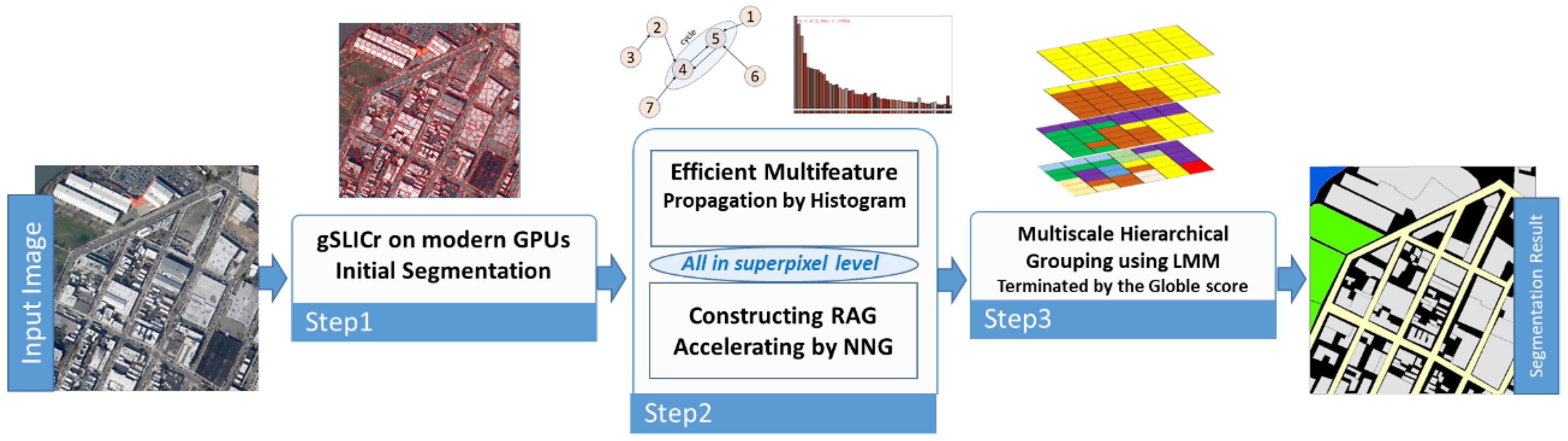
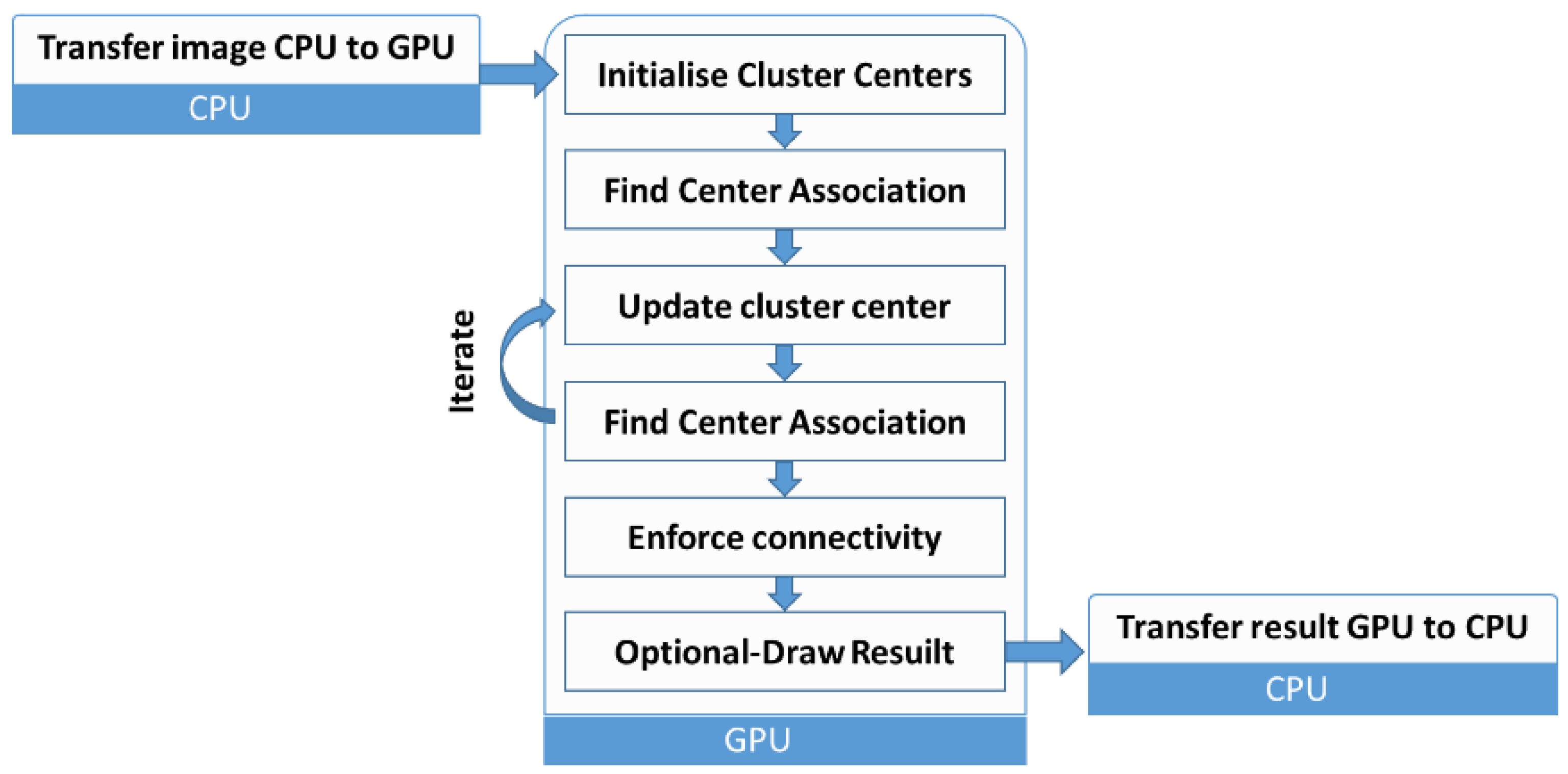
By summarizing the above research, we are trying to further improve the speed and effect of HSR remote sensing image segmentation through GPUs, superpixels, the region merging strategy and multifeature integration. In this paper, we aim to develop a rapid HSR image segmentation system to produce high quality image segments for OBIA. We propose a multiscale and multifeature hierarchical segmentation method (MMHS) for HSR imagery that integrates the superiorities of superpixels and the hierarchical merging method and avoids the disadvantages of these pixel-based methods. In MMHS, our effort starts with a GPU version of the simple linear iterative clustering (SLIC) algorithm [26,31] to quickly obtain initial seed regions (superpixels) by performing over-segmentation. As geometric information is crucial for HSR imagery, multiple features including the spectral, texture, and structural features are taken into consideration to better represent the characteristics of the superpixels. A hierarchical stepwise optimized region merging process (HSWO) [21] using mutual optimal strategy is then performed based on the distance metric to output a set of hierarchical segmentations. Note that to maintain the efficiency of our method, we design image features that are accelerated by histograms and are appropriate for region merging computing. The algorithm can quickly calculate and capture all scales, and we use a global score [38] that reflects intra- and inter-segment heterogeneity information to evaluate the optimal scale selection. The efficiency of the proposed algorithm is verified with six HSR datasets: two aerial orthophoto images and a QuickBird image. By comparing the results with those of other state-of-the-art algorithms, i.e., the WTS algorithm, MS algorithm, and MRS algorithm, it is shown that the proposed MMHS algorithm shows promising performance in terms of both visualization and quantitative evaluation.

There are three main contributions of this work:

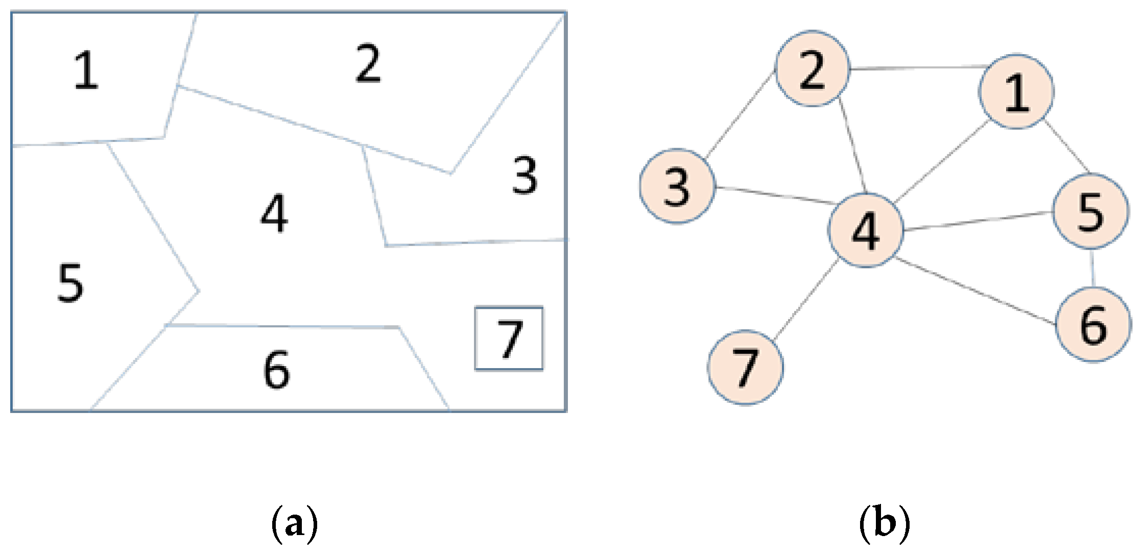
• In this paper, we design a fast and reliable segmentation framework by using the GPU version of a superpixel, the nearest neighbors graph, and carefully designing the image features which can be propagated directly at the superpixel level.
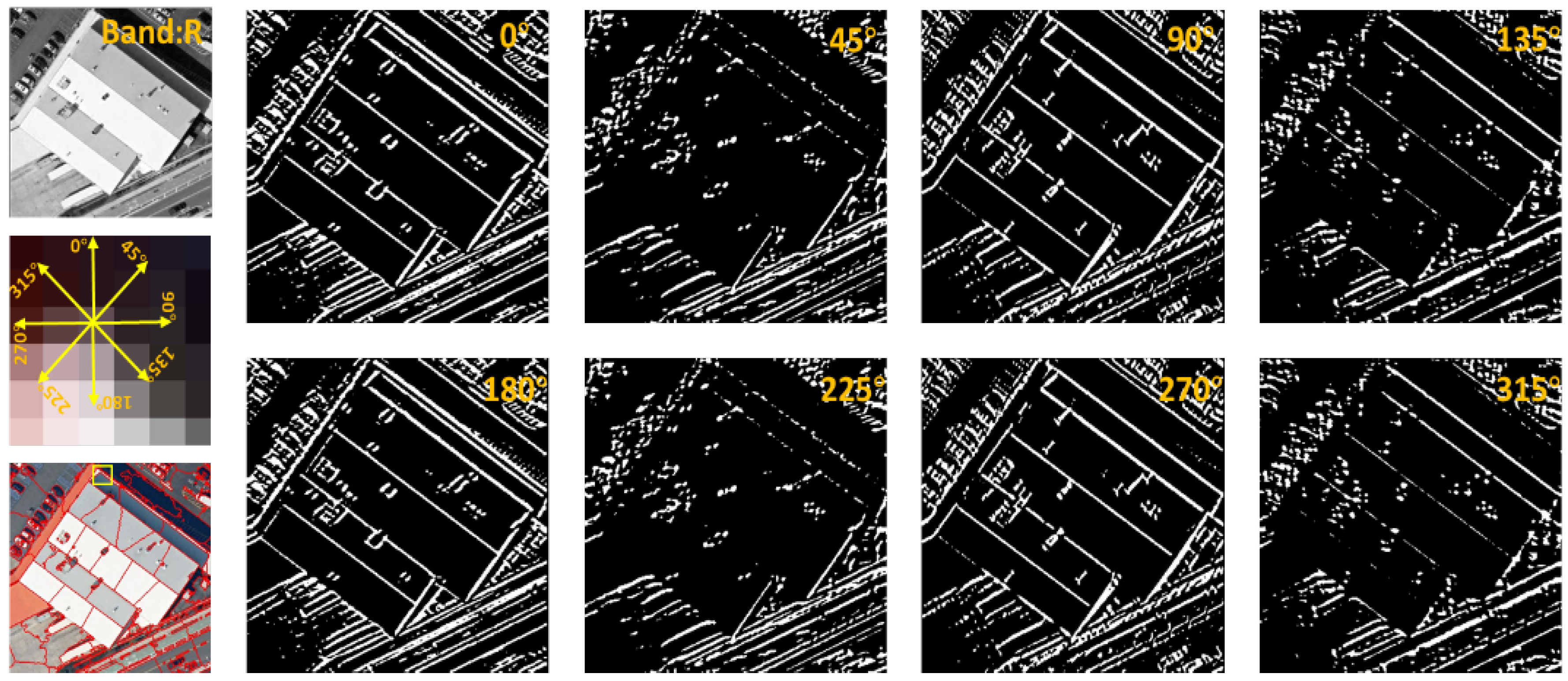
• We also carefully design the multifeature integration of colors, textures, and edges. Each feature is integrated with weighting factors to increase the differences between superpixels. We adjust the corresponding weights to adapt to different HSR remote sensing images.
• Our work attempts to address the selection of optimal scale problem by using a novel global score [38] that reflects intra- and inter-segment heterogeneity information.

The remainder of the paper is organized as follows. In Section 2, the details of the proposed MMHS segmentation method are described. Then, in Section 3, we perform two sets of experiments to evaluate the performance of the proposed method and compare it with the visual contrast and three quantitative indicators. The discussion and conclusions are given in Section 4 and Section 5, respectively.

2. Methodology

Our algorithm considers the following aspects:

• Fast. The goal of MMHS is to generate a set of good segmentation objects for practical remote sensing analysis applications. This algorithm should not be a computational bottleneck, so our algorithm should be fairly fast.
• Multifeature. Regions may form an object because of only colour, only texture, or because parts are enclosed. Therefore, we want to have an adjustable multifeature integration strategy to handle all situations.
• Multiscale. Remote sensing image materials are complex and variable, and objects can occur in any proportion within the image. Therefore, in MMHS, all scales have to be taken into account. This is most naturally achieved by using a multiscale hierarchical algorithm.

The proposed hybrid segmentation method consists of three steps. First, the gSLICr [31] algorithm is used to perform the initial segmentation of the HSR image on modern GPUs, and the number of gSLICr superpixels, compactness, and boundary adhesion are adjusted according to the features of the input HSR image. Second, it connects adjacent superpixels to construct region adjacency graphs for superpixels and computes the similarity between superpixels as RAG edge weights [22]. To speed up the calculation, we use the nearest neighbor graph (NNG) [23] to improve the RAG and adopted a more efficient similarity calculation strategy. Third, multiscale hierarchical region grouping is conducted using local-mutual best region merging (LMM) [17]. In this step, the iterative merging process is applied, and finally, the hierarchical segmentation results are obtained when the merging process is terminated by the given threshold according to the global score [38]. The framework of the segmentation method is shown in Figure 1.

2.1. Superpixel Segmentation and gSLICr

The gSLICr is a GPU implementation of the SLIC algorithm, using the NVIDIA CUDA framework [31], which is the fastest superpixel method available to date. It is simple, efficient, and suitable for real-time operation. The implementation is up to 83× faster than the original CPU implementation of SLIC algorithm [26,31]. We split the implementation into two parts, as shown in Figure 2: the GPU is responsible for most of the processing, with only data acquisition and visualization being left for the CPU.

The following describes the steps of the gSLICr implementation:

• Cluster center initialisation. The seed points are uniformly distributed within the image. If we set the number of superpixels as K and the distance between these superpixels is defined as S, then the seed points are at the center of the superpixel’s position, S = sqrt (N/K), where N is the total number of pixels.
• Updating the cluster center. Generally, we reselect the seed point (n = 3) by choosing a point with the minimum gradient being the initial seed points in an n × n neighborhood of the center point. The minimum gradient point is the center of the nodes.
• Finding the cluster associations. Each pixel in the image determines what its closest cluster is using the 5D distance detailed in the previous section. The search scope is limited to 2S × 2S, which accelerates the convergence of the algorithm. The 5D similarity distance is calculated using a vector, i.e., (l, a, b, x, y). (l, a, b) represents the pixel color value in the CIELAB color space, and (x, y) indicates the position of the pixel. The distance calculation method is as follows:

  $$d_c=\sqrt{{\left(l_j-l_i\right)}^2+{\left(a_j-a_i\right)}^2+{\left(b_j-b_i\right)}^2}$$

  (1)

  $$d_s=\sqrt{{\left(x_j-x_i\right)}^2+{\left(y_j-y_i\right)}^2}$$

  (2)

  $$\mathrm{D}=\sqrt{{\left(\frac{d_c}{m}\right)}^2+{\left(\frac{d_s}{S}\right)}^2},$$

  (3)

  where $d_c$ represents the color distance; $d_s$ represents the space distance; S represents the seed point distance; and m represents the proportion of the color value and spatial information in the similarity calculation. D is the similarity of two pixel points.
• Enforce connectivity. The discontinuous superpixels and undersize superpixels generated in the previous segmentation process are reassigned to adjacent superpixels.

2.2. Superpixel-Based Hierarchical Graph Model Construction

2.2.1. Hierarchical Image Segmentation

The initial oversegmentation of the image was performed by the gSLICr algorithm, and then the image was divided into multiple levels. Then, the image was set as I and the hierarchical segmentation was set as S = {s1, s2, …, sn}. So, the i-th segmentation result of image I was composed of i superpixels, si = {r1, r2, …, ri}. In the process of hierarchical segmentation, the minimum level of the image is over-divided. The image is composed of a large number of small superpixels, and a large superpixel region is generated by region combination to generate a segmentation result of a coarse scale.

Each hierarchical segmentation result was represented by the structure of the graph. Adjacent superpixels had a common boundary. These superpixels and the adjacencies between them were represented by region adjacency graphs, that is, RAG. The superpixel-based graph structure is shown in Figure 3. The superpixel RAG provides a spatial view for the segmented image which facilitates the region merging operation. We used each superpixel as the node vi of the graph, and the neighboring superpixels were connected by the edge ei. We let G = (V, E) be an undirected graph, where V is a set of nodes and V = {v1, v2, …, vn}. E is a set of edges and E = {e1, e2, …, en}. Each edge has a corresponding weight wi, and wi represents the similarity measurements and differences between the adjacent superpixels.

In order to achieve high efficiency, the traditional application of grouping indicators of natural images is often simple, such as regional color mean or variance. HSR remote sensing images have typical spectral diversity characteristics. Due to the wide range of image map coverage, diverse geographical distribution, and complex illumination conditions, HSR images often appear in the “same spectral from different materials and same material with different spectral” phenomenon, often not enough to rely solely on the spectral features to accurately represent the target object. Therefore, to better represent the superpixel region of the HSR image and obtain the best similarity and difference of the neighboring superpixel region, our paper explored a group of simple features that could be efficiently calculated. Both internal and marginal features were considered here. We discuss the details of the features used in our paper below.

2.2.2. Similarity Measures

Our paper used the unified CIELAB color space in the initial over-segmentation algorithm and the same two region merging algorithm. Based on the principles of fast calculation, complementarity, and validity, we integrated color, texture, and boundary features to measure similarity. These measures were all in the [0, 1] range which is beneficial for the combination of these measures. Histogram-based similarity calculations have been widely used [28,34] at the superpixel level. In this paper, we made full use of the advantages of histograms to perform color space quantization and feature similarity calculation.

Color similarity. The CIELAB color space is widely used and has been shown to have significant effects in many applications of computer vision. According to reference [39], regions with high color contrast are more likely to cause visual attention. Therefore, similar to the study in reference [28], we used color-based contrast to calculate the color similarity between different superpixel regions. Typically, the contrast of one pixel is needed to calculate the difference between it and other pixel colors of the image. However, for an 8-bit three-band HSR image, the color type number is ${256}^3$, so the time complexity of direct calculation is too high. To reduce the number of colors and improve computational efficiency, we used a histogram-based method to accelerate the calculation of color similarity. Using the same scheme as that suggested in reference [37], we quantized the number of colors from 256 to 12 in each color band. The number of colors in an image often accounts for only a small part of the entire color space, so we further reduced the number of colors by the histogram; that is, we calculated the color histogram for the input image, retained the high-frequency color covering 95% of the image pixels, and discarded the remaining color, replacing it with the closest color in the histogram. At the same time, the similarity between two adjoining superpixels was calculated based on the contrast of the region, and the color distance between the two superpixel regions, $S_1$ and $S_2$:

$${\mathrm{D}}_C\left(S_1,S_2\right)={\displaystyle \sum }_{i=1}^{n_1}{\displaystyle \sum }_{j=1}^{n_2}f\left(c_1,i\right)f\left(c_2,j\right)\mathrm{D}\left(c_1,i,c_2,j\right),$$

(4)

where $n_1$ and $n_2$ are the total numbers of colors in the superpixel regions $S_1$ and $S_2$, respectively. $f\left(c_1,i\right)$ is the normalized histogram probability of the i-th color $c_1$ in the region $S_1$, and $f\left(c_2,j\right)$ is the normalized histogram probability of the j-th color $c_2$ in the region $S_2$. $\mathrm{D}\left(c_1,i,c_2,j\right)$ represents the distance between the color values of $c_1$, i and $c_2$, j in the LAB color space. Each superpixel area contains only a few kinds of colors, and storing the color histogram of each superpixel according to the color of the entire map is inefficient, so sparse histogram storage and calculations were used.

The color histogram of the merged superpixels was conveniently calculated by the following formula in the process of the hierarchical superpixel regions merging:

$$H_m=\frac{\mathrm{size}\left(S_i\right)\times H_i+\mathrm{size}\left(S_j\right)\times H_j}{\mathrm{size}\left(S_i\right)+\mathrm{size}\left(S_j\right)},$$

(5)

$\mathrm{where}\mathrm{the}\mathrm{size}\left(S_i\right)$ and $H_i$ represent the size and color histogram of the i-th superpixel, respectively. $H_m$ is the color histogram of the merged superpixels.

Texture similarity. Texture is a visual feature that reflects the homogeneity of an image. It is represented by the grayscale distribution of pixels and the surrounding spatial neighborhood. Unlike color similarity, texture similarity is not a pixel-based feature; it requires statistical calculations in areas that contain multiple pixels. This regional statistical feature has advantages such as LBP, SIFT, etc., which are often rotationally invariant and have strong resistance to noise. Here, following the principles of being fast and effective, we used a SIFT-like method to represent texture features. In an over-segmented superpixel region, when the edges are close to each other, the traditional isotropic Gaussian smoothing process will blur the edges. According to the principle of anisotropic Gauss filtering, we selected fast anisotropic Gaussian filtering [40]. As shown in Figure 4, we calculated the anisotropic Gaussian derivative in each of the eight directions for each band using ${\sigma }_v=1,{\sigma }_u=2$ on modern GPUs. Then, we extracted a texture histogram using a bin size of 10 for each direction. First, counted the gradient maximum and minimum values in each direction and obtained the bin interval of the histogram. Second, the over-segmentation assigns a superpixel label for each pixel. So, each pixel in a superpixel region was traversed, the difference between it and the minimum value was calculated, and the interval index number of the pixel in the histogram was obtained. Then, the histogram of the corresponding superpixel region was obtained until all pixels had been traversed. Third, the eight histograms were combined and normalized according to the size of the superpixel.

Therefore, if the HSR image had three color channels, the texture feature of the i-th superpixel region was represented as a 240-dimensional (8 × 10 × 3) vector $T_i=\left\{t_i^1,t_i^2,\dots ,t_i^n\right\}$, n = 240. The similarity distances of neighboring superpixel regions $S_1$ and $S_2$ were obtained by the normalized histogram intersections:

$${\mathrm{D}}_T\left(S_1,S_2\right)=dist\left(T_1,T_2\right)={\sum }_{i=1}^n\left|t_1^i-t_2^i\right|,$$

(6)

where $T_1=\left\{t_1^1,t_1^2,\dots ,t_1^n\right\}$, $T_2=\left\{t_2^1,t_2^2,\dots ,t_2^n\right\},$ and n is the dimension of the texture feature. So, the texture similarity was used to calculate the Manhattan distance of the corresponding two n-dimensional vectors. The texture histograms were efficiently propagated through the hierarchy in the same way as the color histograms.

Then, in the proposed method, the color and texture similarity distance metrics were combined in a weighted manner. The weights were adjusted according to the distribution of colors and textures. For example, a forest scene is more homogeneous, in which the spectral values for the different types of land cover are quite similar. An urban area is more heterogeneous, where different types of land cover can have very different spectral characteristics. So, if the homogeneity of the feature distribution is better and the color values are quite similar, the texture weights should be larger, and the texture weights with lower homogeneity should be smaller. For complex HSR remote sensing images, we need a balance between the texture and color weights. Therefore, we used the adjustment of weights to achieve a reasonable representation of regional features.

$${\mathrm{D}}_{ij}=\alpha ·{\mathrm{D}}_C\left(S_i,S_j\right)+\beta ·{\mathrm{D}}_T\left(S_i,S_j\right),$$

(7)

where ${\mathrm{D}}_C\left(S_i,S_j\right)$ and ${\mathrm{D}}_T\left(S_i,S_j\right)$ are the color and texture similarity distances of two adjacent superpixels, $S_i$ and $S_j$. α and β are their respective adjustable two weight factors.

Edge weighted region similarity. The combination of color and texture weighting can express the characteristics of the area well, but it is possible to generate objects with zig-zag contours when combined [35]. The use of boundary constraints can make the shape of the merged object more compact and reasonable. We used the length information of the common boundary between adjacent superpixel regions to introduce a boundary weight in Equation (8). That is, when the color and texture features are similar, the common boundary is longer and it is more likely that the two regions will merge. Specifically, the definition is as follows:

$${\mathrm{D}}_{ij}=\exp \left(\frac{-L_E\left(S_i,S_j\right)}{{\sigma }_e^2}\right)\left(\alpha {\mathrm{D}}_C\left(S_i,S_j\right)+\beta {\mathrm{D}}_T\left(S_i,S_j\right)\right)$$

(8)

where $L_E\left(S_i,S_j\right)$ is the common boundary length between the regions $S_1$ and $S_2$, and ${\sigma }_e$ is a parameter used to adjust the boundary weights by adjusting ${\sigma }_e$ to achieve the effect of controlling public boundary constraints.

2.3. Hierarchical Grouping

After establishing adjacency relations and similarity measures in all over-segmented regions, superpixel region merging is an important process that ultimately achieves finer segmentation. The commonly used methods are EGB [12] and HSWO [21], which continuously iteratively merge the small areas that meet the conditions through the set merge criteria from bottom to top until some threshold is satisfied. In each merging step, there are a large number of divided regions, and each region has multiple adjacent regions. Therefore, the number of RAG nodes and the number of edges are enormous. The computational complexity of searching for the best merged object from all RAG nodes is very large.

Local-mutual best region merging (LMM). Baatz [17] proposed local-mutual best region merging (LMM) which can be applied if the combined index is less than the threshold and A and B are the best-fit neighbors to each other. To adopt the LMM strategy, the NNG [23] was introduced on the basis of RAG to accelerate the merging algorithm. NNG is a directed graph which is a collection of pointed edges. A directed edge joins from each node. Based on the LMM strategy, this edge points to the node’s best merged object. In NNG, which is shown in Figure 5, the pair of regions that are most similar to each other must belong to pairs connected by circular arcs. If there are N nodes in the NNG, in the worst case scenario, the number of circular arcs will be N/2. Therefore, RAG only records the relationship between adjacent regions and does not need to be responsible for the cost of the merger between nodes. LMM is performed in NNG to search for the best merged area. NNG has a smaller search space and greatly reduces the amount of data. In graph theory, the NNG is also called a minimal spanning tree (MST). It has been well proven in many studies, such as references [34,41].

Multiscale Hierarchical Grouping. Considering the complexity of the features of HSR images, obtaining optimal image segmentation results is a problem of scale selection. One of the most powerful segmentation methods is the scale set representation introduced by Guigues et al. [42], which builds a hierarchy of regions or a single suite of partitions. As the optimal partitioning of an image depends on the application, our method proposes to keep all partitions obtained at all scales, from the pixel level until the complete image. As each feature may have different segmentation scales to facilitate different scale requirements, we adopted a multiscale hierarchical region grouping method. Using a greedy algorithm, we were able to obtain the segmentation results for all scales until the entire image became a single area. The graph-based multiscale hierarchical grouping algorithm is described in

Table 1. Multiscale hierarchical grouping.

Input: RAG [22] and NNG [23] of the initial over-segmentation image; The threshold for grouping: T, weight of the color: $\alpha$, texture: $\beta$, boundary constraint parameters: ${\sigma }_e$;

Output: The merging result

1. Set i = 0, Calculate the edge weights of RAG and NNG ei by Equation (8) 2. Find the minimum weight edge in the current NNG closed loop for the i-th hierarchy 3. If e < T, use local-mutual best region merging (LMM [16]) 4. Update RAG, NNG, and the cycle 5. Set i = i + 1 6. Return to Step 2, repeat LMM, until there is no cycle.

. The whole process is like hierarchical clustering. We drew a hierarchy of dendrograms to represent the entire multiscale hierarchical grouping process that is shown in Figure 6.

In the process of multilevel hierarchical merging, the similarity distance measure makes full use of the advantages of the histogram. For each feature of the merged new region, we only needed to use the features of the two regions before the merge. These details further ensured the efficiency of our algorithm.

3. Experiments and Analysis

Here, we describe the testing the proposed MMHS algorithm on six HSR remote sensing datasets from the New York State High Resolution Digital Orthoimagery Program (NYSDOP) and the ISPRS Potsdam Semantic Labeling dataset [43]. In the first experiment, we tested the gSLICr, which is a CUDA-based GPU version SLIC method [31], with well-known image over-segmentation algorithms—the efficient graph-based image segmentation (EGB) method and the SLIC algorithm—to check the effect and efficiency of the initial superpixel segmentation. In the second experiment, we compared three state-of-the-art algorithms: the multiresolution segmentation algorithm (MRS) in the commercial software eCognition9; the mean shift algorithm (MS); and the watershed transform segmentation algorithm (WTS). All algorithms were programmed by C++ and tested on a Windows 10 64-bit with Intel CPU i5-6500 at 3.2 GHz and an NVIDIA GeForce GTX 1060 6 GB. There are several free parameters in the proposed MMHS algorithm: the weight of the color $(\alpha )$, the texture ($\beta$), and the boundary constraint parameters $({\sigma }_e),$ and we present the results of tests of their sensitivity in Section 3.4. In Section 3.5, we present the analysis of the effects of segmentation scale selection and determine the optimal number of segments for experimental images. The WTS and MS algorithms came from the open source image processing library OpenCV.

3.1. Description of Experimental Datasets

The experimental dataset from NYSDOP contained a set of HSR images in the US state of New York, as shown in

Table 2. The list of test images.

Image	Platform	Spatial Resolution (m)	Size (Pixel)	Bands	Landscape
T1	QuickBird	0.6	2324 × 2324	NIR, R, G, B	Urban residential area
T2	Aerial	0.3	2979 × 2979	NIR, R, G, B	Urban area
T3	Aerial	0.3	6000 × 6000	NIR, R, G, B	Rural area
T4	Aerial	0.05	6000 × 6000	NIR, R, G, B	Urban area
T5	Aerial	0.05	6000 × 6000	NIR, R, G, B	Urban area
T6	Aerial	0.05	6000 × 6000	NIR, R, G, B	Urban area

and Figure 7, including QuickBird and aerial images with spatial resolution ranges from 0.6 m (T1) to 0.3 m (T2 and T3), respectively. Images T4, T5, and T6 came from the ISPRS dataset [43]. The ISPRS Potsdam dataset is an open benchmark dataset which consists of 38 ortho-rectified aerial IRRGB images (6000 × 6000 px), with a 5 cm spatial resolution and corresponding ground truth.

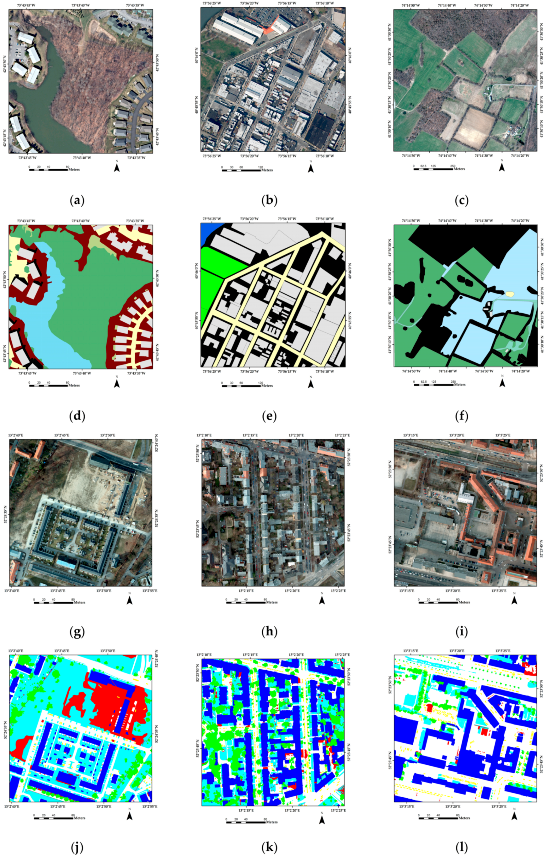
Image T1 was an urban residential area located in Albany County. Image T2 covered a typical urban landscape with dense buildings, criss-crossing roads, and a few grassland spaces in Manhattan, New York City. Image T3 recorded a rural area with spatial dimensions of 6000 × 6000 pixels in Montgomery County. Images T1 and T2 were 2324 × 2324 and 2979 × 2979, respectively and contained pixels in four spectral bands: red, green, blue, and near-infrared. Images T4, T5, and T6 were from the urban area of Potsdam, Germany. Their color composite images are shown in Figure 7a–l, which are the corresponding benchmark images.

To fully evaluate the computational efficiency and segmentation accuracy of the proposed algorithm under different conditions, we used two different sources of HSR images covering a variety of features, such as buildings, roads, vegetation, grasslands, and lakes. Each experimental image contained monotonous and intensely mixed complex spectra, textures, and shape features.

3.2. Evaluation Criteria and Experiment Setup

For the purpose of evaluating our method more objectively, the evaluation indices principle used was different from our segmentation algorithm. We used the supervised and unsupervised segmentation assessment methods. The segmentation index was evaluated from many aspects, such as under-segmentation, over-segmentation, shape, heterogeneity and homogeneity. We evaluated the segmentation results for all experiments from the following seven indicators of three types: first, the normalized weighted variance (wVar), the normalized global Moran index (MI), and the global score (GS) [38]; second, the potential segmentation error (PSE), the number of segments ratio (NSR), and the Euclidean distance 2 (ED2) [44]; and third, the object level consistency error (OCE) [45]. They are all shown in

Table 3. Overview of the selected segmentation accuracy metrics. $v_i$ is the variance and $a_i$ is the area of segment i; $s_j$ defines the area of corresponding ground truth segments (j); n is the total number of segments, m denotes the number of reference polygons, and v denotes the number of corresponding matching segments, ${\omega }_{ik}$ is a measure of the spatial proximity, $y_i$ and $y_k$ are the mean spectral values of regions $R_i$ and $R_k$, and $\overline{\mathrm{y}}$ is the mean spectral value of the image, $norm$ is the normalization. $I_g$ and $I_s$ are the reference image and the segmentation image, respectively, $\overline{\delta }$, $W_{ji}$, and $W_j$ are the delta function and weight coefficients, respectively.

Segmentation Accuracy Metric	Formula	Domain	Ideal Value	Original Reference
$\omega Va{r}_{norm}$	$\omega Var={\frac{{\sum }_{i=1}^n{a}_i\ast v_i}{{\sum }_{i=1}^n{a}_i}}_{norm}$	$\left[0,1\right]$	0	Johnson et al. [38]
${\mathrm{MI}}_{norm}$	$\mathrm{MI}={\frac{n{\sum }_{i=1}^n{\sum }_{k=1}^n{\omega }_{ik}\left(y_i-\overline{\mathrm{y}}\right)\left(y_k-\overline{\mathrm{y}}\right)}{{\sum }_{i=1}^n{\left(y_i-\overline{\mathrm{y}}\right)}^2\left({\sum }_{i\ne k}\sum {\omega }_{ik}\right)}}_{norm}$	$\left[0,1\right]$	0	Johnson et al. [38]
$\mathrm{GS}$	$\mathrm{GS}=\omega Va{r}_{norm}+{\mathrm{MI}}_{norm}$	$\left[0,2\right]$	0	Johnson et al. [38]
$\mathrm{PSE}$	$\frac{\sum \left|s_j-a_i\right|}{\sum \left|a_i\right|}$	$\mathrm{PSE}>0$	0	Liu et al. [44]
$\mathrm{NSR}$	$\frac{\left|m-v\right|}{m}$	$\mathrm{NSR}>0$	0	Liu et al. [44]
$\mathrm{ED}2$	$\sqrt{{\mathrm{PSE}}^2+{\mathrm{NSR}}^2}$	$\mathrm{ED}2>0$	0	Liu et al. [44]
$\mathrm{OCE}$	$E_{g,s}\left(I_g,I_s\right)={\displaystyle \sum _{j=1}^m}\left[1-{\displaystyle \sum _{i=1}^n}\frac{\left|s_j\cap a_i\right|}{\left|s_j\cup a_i\right|}\times W_{ji}\right],$ $W_{ji}=\frac{\overline{\delta }\left(\left|s_j\cap a_i\right|\right)\left|a_i\right|}{{\sum }_{k=1}^n\overline{\delta }\left(\left|s_j\cap a_k\right|\right)\left|a_k\right|},W_j=\frac{\left|s_j\right|}{{\sum }_{i=1}^m\left|a_i\right|}$ $\mathrm{OCE}\left(I_g,I_s\right)=\min \left(E_{g,s},E_{sg}\right)$	$\left[0,1\right]$	0	Polak et al. [45]

.

The global score (GS) is calculated by adding the normalized weighted variance (wVar) and the normalized global Moran index MI. The variance of the segmented region can reflect the relative degree of homogeneity of the region and is often chosen as the intra-segment goodness measure. wVar is a global calculation based on the area of the segmented region which makes large segments have more impact on global homogeneous. Global Moran’s I is a spatial autocorrelation measure that can characterize the degree of similarity between an area and its neighbors and can be used as a good indicator of segmentation quality assessment. Brian Johnson [38] chose it as the inter-segment global goodness measure in the calculation of the global score (GS). Low Moran’s I values indicate high inter-segment heterogeneity, which is desirable for image segmentation. So, in theory, a good segmentation result should have a low global score.

The Euclidean distance 2 (ED2) is a composite index that considers both geometric and arithmetic discrepancies proposed by Liu et al. [44]. He improved the Euclidean distance 1 based on this under-segmentation (US) indicator and proposed the Potential Segmentation Error (PSE) and Number of Segments Ratio (NSR). The PSE is the ratio between the total area of under-segments and the total area of reference polygons. The range of the PSE is [0, +∞]. When the best value is 0, the reference object does not have under-segmentation. NSR is defined as the absolute difference in the number of reference polygons and number of corresponding segments divided by the number of reference polygons. When the NSR value is 0, all reference objects and matching objects are in one-to-one correspondence, and the segmentation effect is the best. The larger the NSR value is, the more the one-to-many or many-to-one matching quantity relationships there are, indirectly indicating that the over-segmentation or under-segmentation phenomenon is more serious. ED2 is calculated by the combination of PSE and NSR. In a two-dimensional PSE–NSR space, the ED2 index is the most reliable when NSR and PSE are the same magnitude, and a small ED2 value can represent good segmentation quality.

By studying two variants of the martin error measure, the global consistency error (GCE), and the local consistency error (LCE), the object-level consistency error (OCE) was proposed by Polak [45]. By comparing the size, shape, and position at the object level on the segmented image and the ground truth image, the OCE can fairly penalize both over- and under-segmentation. At the same time, it retains the properties of being normalized, symmetric, and scale invariant, respectively.

In the algorithm comparison experiments, we set corresponding parameters for different algorithms to obtain fine precision and speed. In Experiment 1, we chose the first Albany QuickBird HSR image as our experimental data. The parameters of EGB algorithm were set as sigma = 0.5, K = 500, and min = 50. The SLIC segmentation parameters were as follows: number of superpixels = 1000, compactness factor = 20, and number of iterations = 10. The parameters of the gSLICr algorithm were as follows: number of superpixels = 1000, compactness factor = 0.6, and number of iterations = 10. In the second experiment, we compared the segmentation algorithms on these three HSR datasets. The parameters of each algorithm on the corresponding data set included eCognition MRS (FNEA) parameters of shape = 0.1/0.2/0.3/0.2/0.1/0.2, compactness = 0.7/0.5/0.5/0.5/0.6/0.5, and scale = 300/500/450/1300/1500/1400. The parameters of the MS algorithm were set as follows: spatial bandwidth = 14/10/8/7/10/7 and color bandwidth = 4/5/46.5/8/4.5. For our segmentation, the parameters were α = 0.4/0.5/0.4/0.4/0.5/0.4, β = 0.6/0.4/0.6/0.6/0.5/0.6, and ${\sigma }_e^2=0.4/0.3/0.5/$0.5/0.4/0.4. The numbers of segments were 74, 105, 84, 93 and 87, respectively. The above parameters of MRS and MS were set by the results of many experiments and experience. The three parameters of our algorithm and the optimal number of segments were obtained by the analyses in Section 3.4 and Section 3.5, respectively.

3.3. Comparative Results and Analysis

3.3.1. First Experiment

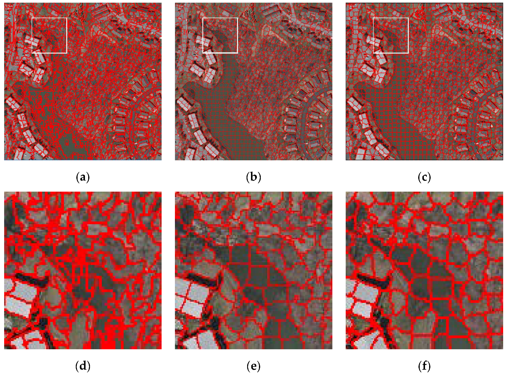
Experiment 1 was the initial over-segmentation experiment conducted on the Albany QuickBird HSR image. Figure 8a–c and

Table 4. Comparison of initial segmentation.

Methods	EGB	SLIC	gSLICr
Runtime	142.1 s	187.5 s	0.11 s
Number of segments	1498	1500	1500

display the over-segmentation results and the number of segments as well as the runtimes of EGB, SLIC and gSLICr.

By comparing the three algorithms from the results shown in

Table 5. Quantitative assessment results of the Albany QuickBird image (T1).

Experiment		Segmentation Results and Accuracy
		Runtime	Segments Number	wVar	MI	GS	NSR	PSE	ED2	OCE
T1	WT	73 s	631	0.4022	0.0614	0.4636	14.833	12.380	19.321	0.947
	MS	244 s	104	0.4328	0.1703	0.6031	2.874	1.490	3.237	0.874
	MRS	30.5 s	90	0.0387	0.3182	0.3569	1.232	2.694	2.9623	0.9143
	MMHS	0.468 s	74	0.2246	0.1086	0.3333	0.9685	1.866	2.1024	0.8592

, it can be observed that the runtimes of EGB, SLIC, gSLICr were 142 s, 187.5 s, and 0.11 s, respectively. At the same time, the numbers of segments were 1498, 1500 and 1500, respectively. Each over-segmented object was a superpixel. The fewer the number of superpixels, the lower the consumption time was. It can be clearly seen that the gSLICr method had the highest efficiency when compared to the EGB and SLIC methods, and with an equal number of superpixels, the time consumption was only one thousandth of that of the former. As shown in Figure 8a–c, the superpixels generated by the three methods all had good boundary adhesion. Compared with the EGB method, the superpixels generated by the SLIC and gSLICr methods were more compact and tidy. The SLIC superpixels and gSLICr superpixels produced similar results. As shown by the enlargement of Figure 8d–f, the algorithm EGB was greatly affected by the speckle noise which caused the shape of the superpixel to be more cluttered and there was no boundary of the surface objects attached. The SLIC algorithm had a uniform superpixel shape and good boundary adhesion. The gSLICr method not only inherits the advantages of the SLIC, but the local detail of the segmentation is also better. For example, in Figure 8f, the remains of the smaller region still have a well attached boundary. Therefore, the gSLICr algorithm not only has great advantages in regard to time performance, but it also performs better than the EGB and SLIC algorithms in terms of number of superpixels, boundary adhesion, and noise resistance.

3.3.2. Second Experiment

The comparison of MMHS with other segmentation methods was conducted on the six test images: the Albany QuickBird image (T1), the Manhattan aerial image (T2), the Montgomery aerial image (T3), and three Potsdam aerial images (T4, T5, T6). Figure 9, Figure 10 and Figure 11 show the segmentation results of WT, MS, MRS, MHS and MMHS, respectively. The red lines represent the boundaries of segmentation. Table 5,

Table 6. The quantitative assessment results of the Manhattan aerial image (T2).

Experiment		Segmentation Results and Accuracy
		Runtime	Segments Number	wVar	MI	GS	NSR	PSE	ED2	OCE
T2	WT	156.7 s	1388	0.2373	0.5907	0.8280	13.878	7.744	15.892	0.9802
	MS	374.2 s	92	0.4229	0.4167	0.8396	1.3402	7.4310	7.5508	0.9805
	MRS	43.2 s	129	0.3518	0.5196	0.8714	3.9821	3.9299	5.5948	0.9616
	MMHS	0.874 s	105	0.4045	0.3603	0.7648	2.7475	4.2556	5.0657	0.9597

and

Table 7. The quantitative assessment results of the Montgomery aerial image (T3).

Experiment		Segmentation Results and Accuracy
		Runtime	Segments Number	wVar	MI	GS	NSR	PSE	ED2	OCE
T3	WT	350.4 s	344	0.2381	0.0993	0.3374	1.0364	7.6285	7.6986	0.9682
	MS	11484 s	48	0.0643	0.3983	0.4626	0.0545	2.3157	2.3163	0.9636
	MRS	198 s	72	0.2006	0.1199	0.3205	1.3393	7.0507	7.1767	0.9405
	MMHS	2.199 s	84	0.2412	0.0281	0.2693	0.4561	1.6595	1.7211	0.9262

display the quantitative assessment results: the segmentation runtime, weighted variance (wVar), Moran index (MI), the global score (GS), the potential segmentation error (PSE), the number of segments ratio (NSR), the Euclidean distance 2 (ED2), and the object-level consistency error (OCE) for WT, MS, MRS and MHS. Our algorithm results are shown in bold.

The segmentation results of T1 produced by the four methods are presented in Figure 9a–d. According to a visual assessment, it can be seen that our MMHS method had better results when compared with other three approaches. The WTS algorithm produced large-scope over-segmentation on the entire image range. At the same time, the MS and MRS were over-segmented in the forest and lake areas, respectively. This is because these segmentation method algorithms based on local changes between neighboring pixels are sensitive to boundary changes in areas where the internal spectrum and gradients change significantly. The MS and MRS algorithms introduce spatial and shape parameters, respectively. Although partial over-segmentation is reduced, it is difficult to achieve optimal segmentation in the overall result. Therefore, in Figure 9b, the MS algorithm led to under-segmentation in both the upper left road area and in the lower right road area. We proposed the superpixel-based MMHS algorithm, which partly overcomes the problem of over-segmentation in the pixel-based methods. The reason for this may be that the superpixels are much less affected by the local error variation, and because the MMHS has the flexibility to choose the best segmentation result.

The quantitative evaluation results of T1 are shown in Table 5. It can be seen from the quantitative comparison that our algorithm had obvious advantages. From Table 5, we can see that, in terms of running time, our algorithm was superior to other algorithms by more than 10 times because of the application of superpixels, GPU acceleration, and an efficient similarity calculation strategy. Among the quantitative evaluation indices, GS is an unsupervised image segmentation evaluation index, and ED2 and OCE are supervised image segmentation evaluation indices. A comparison of the GS values for the WTS, MS, MRS, and MHS segmentations showed that the MMHS image segmentation had the lowest average GS (0.3333). This means that the MMHS segments were, on average, most homogeneous internally and most different from their neighbors. The WTS and MS methods had higher wVar values because their segmentation results retained more detailed objects. The MRS segmentation result had the highest MI value indicating that the segmentation was not enough and there were incorrect segmentations. We computed the PSE, NSR, and ED2 by comparing their segmentation results with the ground truth vectors. The PSE of WTS algorithm had a large value (12.380) which implies a significant degree of under-segmentation. The NSR of WTS algorithm also had a larger value (14.833), indicating a dominant one-to-many relationship and a significant degree of oversegmentation. The ED2 values of the WTS algorithm, the MS algorithm, the MRS algorithm, and the MMHS algorithm were 19.321, 3.237, 2.9623 and 2.1024, respectively. The ED2 value of the MMHS algorithm was lower than the ED2 values of the WTS algorithm, the MS algorithm, and the MRS algorithm, showing that the MMHS algorithm was better than the other two algorithms. The OCE value of the MMHS algorithm was the lowest of all the algorithms, showing that the segmentation result produced using the MMHS algorithm was the best among the three algorithms. Therefore, we know that at the object level, the shape, location, size, and existence of our MMHS segment region has the best consistency with the ground reference.

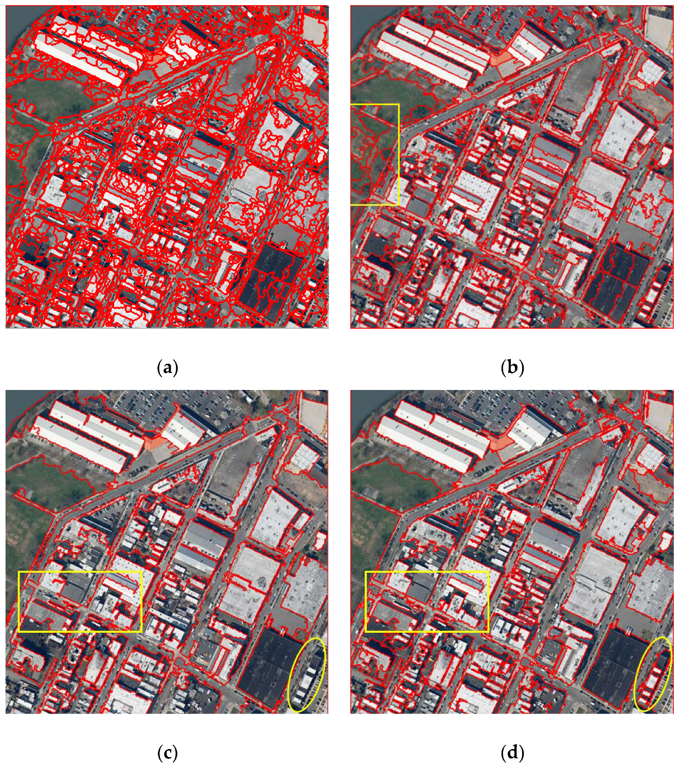
For the T2 image, there were many factories with complex roofs and roads with no obvious boundaries. The segmentation map and the quantitative result of the image T2 are shown in Figure 10 and Table 6, respectively. In the first row, the over-segmentation of the WTS algorithm is extremely serious and the MS algorithm also has a lot of over-segmentation in the building roof and lawn areas. On the other hand, the multiresolution segmentation order strategy in the MRS also worked, which achieved better segments. However, it was still not better than MMHS in terms of the boundaries of roofs. As MMHS adopts gSLICr superpixels with good boundary adhesion and the LMM strategy, our method obtained a multiscale performance where both lawn areas with a large scale and building shadow with small scale could be segmented into the same region. For example, a narrow strip of buildings in the lower right corner was segmented out by MMHS, whereas the MRS methods could not distinguish it very well.

From the segmentation assessment in Table 6, it can be seen that the MMHS segmentation time tended to be basically the same as T1. The four algorithms had larger assessment values of GS, ED2, and OCE than those of T1, indicating that the overall T2 segmentation effect was not as good as T1. Compared with WTS, MS, and MRS, the GS (0.7648), ED2 (5.0657), and OCE (0.9597) of MMHS had obvious advantages which is consistent with our visual assessment.

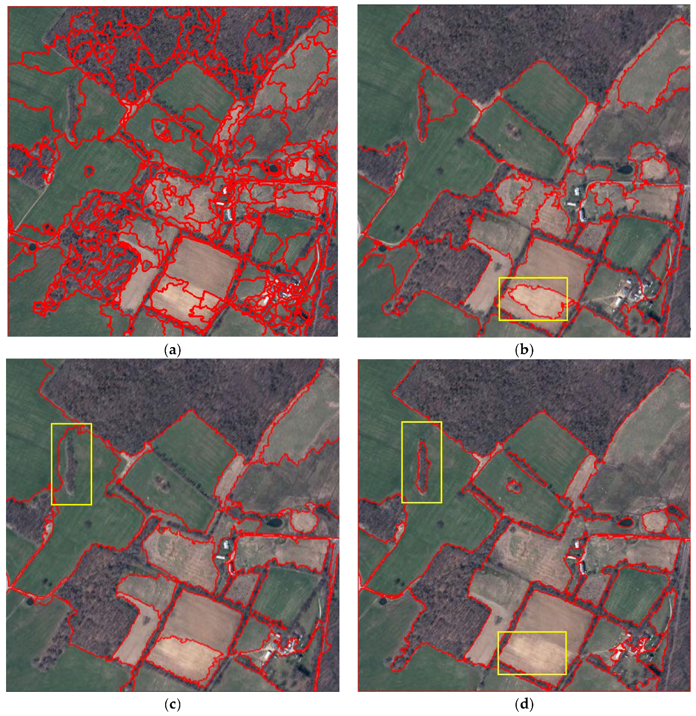
The segmentation map of image T3 is shown in Figure 11, and the quantitative results are given in Table 7. To further evaluate the segmentation efficiency of different methods, unlike T1 and T2, the size of T3 was 6000 × 6000, and T3 had a large uniform texture area and a small scale texture change area. As can be seen from Figure 11 and Table 7, apart from WTS, all three methods had good segmentation results and accuracy. Regarding the running time, MMHS achieved a satisfactory 2.2 s, which was far better than the other three methods. For segmentation quantitative indicators, the GS, ED2 and OCE value of the MMHS were the lowest, which means that the segmentation results of the MMHS were obviously better than the other three. From Figure 11, it can be seen that when compared with MS and MRS, MMHS showed better segmentation performance in the tiny woodland and bare land because the compact superpixel merging provided good boundary adhesion, and it also reduced the impact of noise. The reason for this is that WTS, MS, and MRS are all bottom-up pixel-based methods, of which the merging processes are determined by local homogeneity; therefore, the results are sensitive to details such as color, texture, shape, and noise. Likewise, the scale problem of segmentation is also difficult to solve.

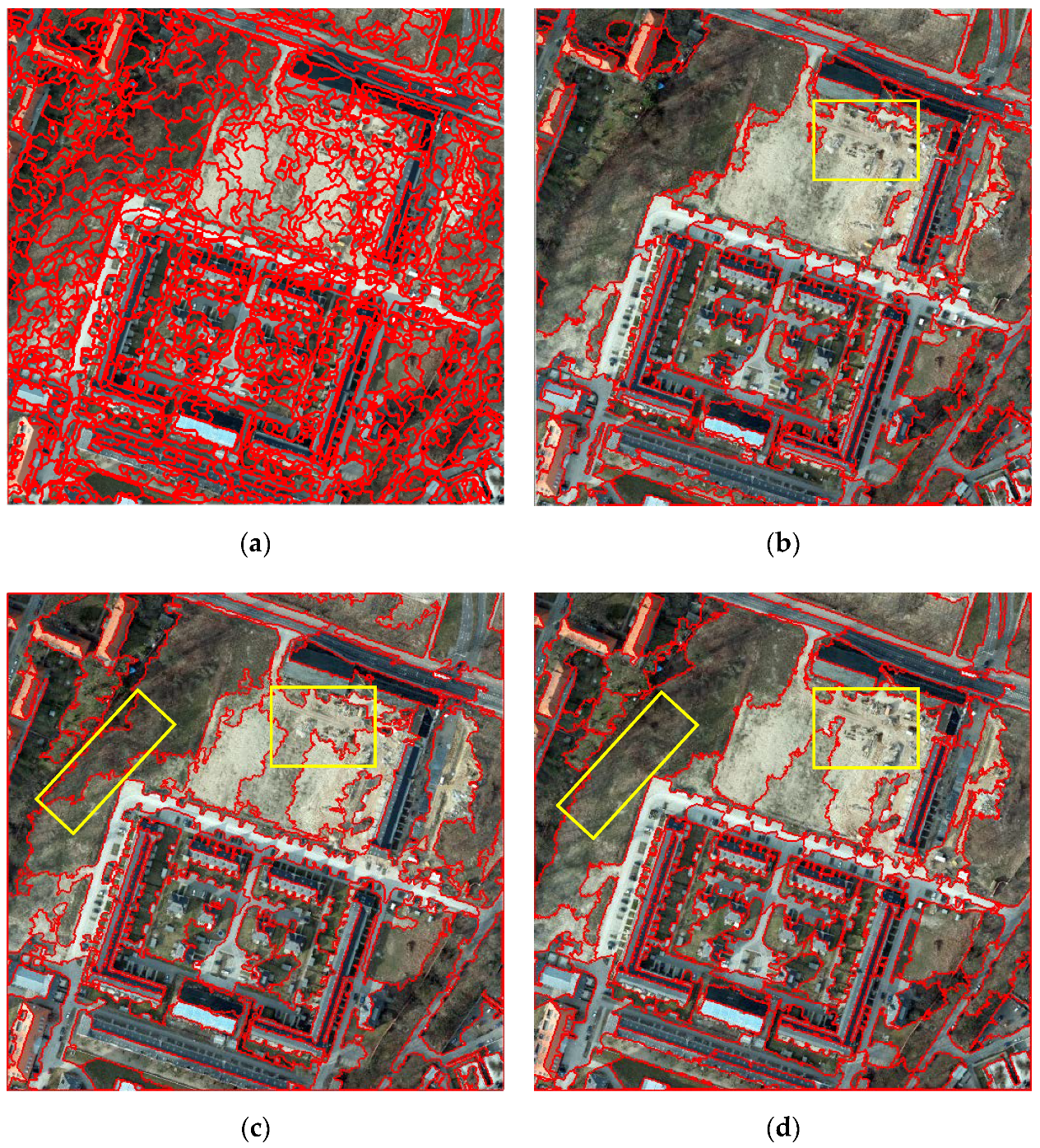
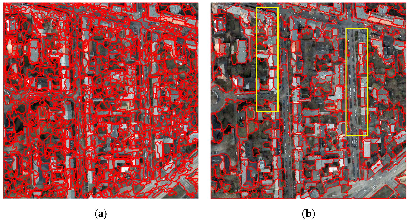
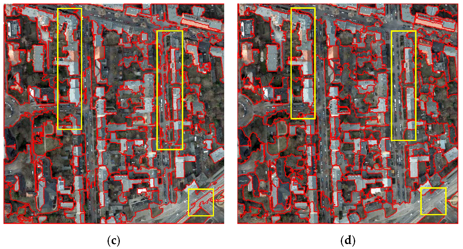
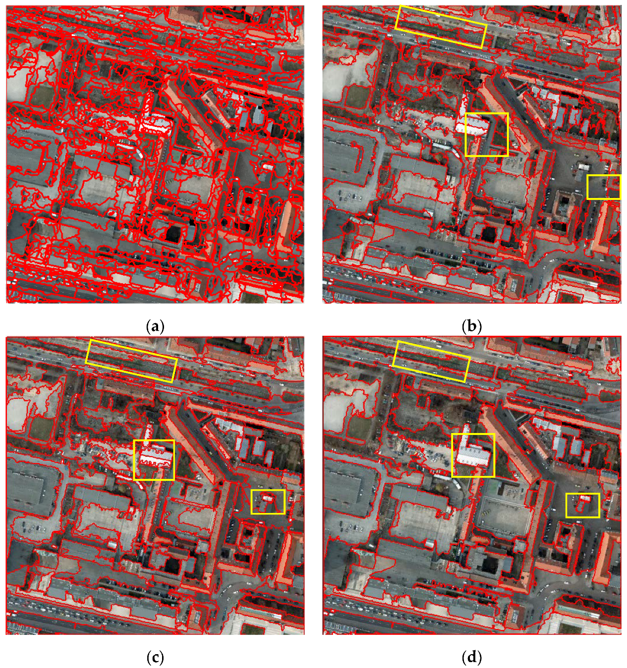
The fourth, fifth, and sixth experimental data were from the urban area of Potsdam, Germany. The segmentation result maps and the quantitative evaluation indicators are shown in Figure 12, Figure 13 and Figure 14, and

Table 8. The quantitative assessment results of the Potsdam aerial image (T4).

Experiment		Segmentation Results and Accuracy
		Runtime	Segments Number	wVar	MI	GS	NSR	PSE	ED2	OCE
T4	WT	486.88 s	1277	0.4056	0.3423	0.7479	5.4309	9.8256	11.226	0.9708
	MS	17721 s	70	0.3782	0.2941	0.6723	3.2279	7.6359	8.2901	0.9541
	MRS	228.6 s	90	0.3109	0.2089	0.5198	2.8350	3.9162	4.8347	0.9566
	MMHS	2.570 s	84	0.3270	0.1546	0.4816	2.6653	2.0308	3.3508	0.9303

,

Table 9. The quantitative assessment results of the Potsdam aerial image (T5).

Experiment		Segmentation Results and Accuracy
		Runtime	Segments Number	wVar	MI	GS	NSR	PSE	ED2	OCE
T5	WT	545.3 s	1327	0.6132	0.1943	0.8075	7.9344	11.082	13.630	0.9811
	MS	19051 s	112	0.4833	0.3021	0.7854	4.8023	8.7534	9.9842	0.9725
	MRS	233.4 s	80	0.4309	0.3164	0.7473	4.0418	5.0773	6.4896	0.9606
	MMHS	2.730 s	93	0.3798	0.2411	0.6209	4.2231	3.8093	5.6873	0.9498

and

Table 10. The quantitative assessment results of the Potsdam aerial image (T6).

Experiment		Segmentation Results and Accuracy
		Runtime	Segments Number	wVar	MI	GS	NSR	PSE	ED2	OCE
T6	WT	524.9 s	986	0.5309	0.2469	0.7778	6.5289	8.9743	11.098	0.9735
	MS	18,545 s	162	0.4832	0.3401	0.8233	4.5581	7.0698	8.4118	0.9622
	MRS	230.1 s	84	0.3632	0.3008	0.6640	2.4725	3.8894	4.6088	0.9590
	MMHS	2.670 s	87	0.3498	0.2746	0.6244	2.7466	2.2903	3.5762	0.9461

. Overall, our algorithm still showed better segmentation result than the other three methods in the three large and complex urban image datasets. In terms of segmentation accuracy, the GS, ED2, and OCE values of our MMHS algorithm were the lowest. From the perspectives of Figure 12, Figure 13 and Figure 14, respectively, the WTS algorithm produced severe over-segmentation, and the segmentation quality was the poorest. Both MS and MRS algorithms were able to segment images better, but in complex urban areas, such as the corresponding yellow marked areas (some houses, bare land, roads, etc.), the segmentation effects were greatly affected. Our algorithm showed better segmentation performance in these areas. This is because our algorithm combines details such as color, texture, boundary, and noise in the entire segmentation process. In complex urban areas, any detail information is sufficient to affect the feature representation. In terms of segmentation speed, our algorithm showed great advantages because we used GPU-based superpixels and well-designed similarity computing strategies. For the T4, T5 and T6 datasets, the MS algorithm took the most time, so it could not be tested normally. The WTS took about 500 s, and the MRS took about 200 s. Our algorithm segmentation speed was about 2 s, which is 100 times faster than MRS.

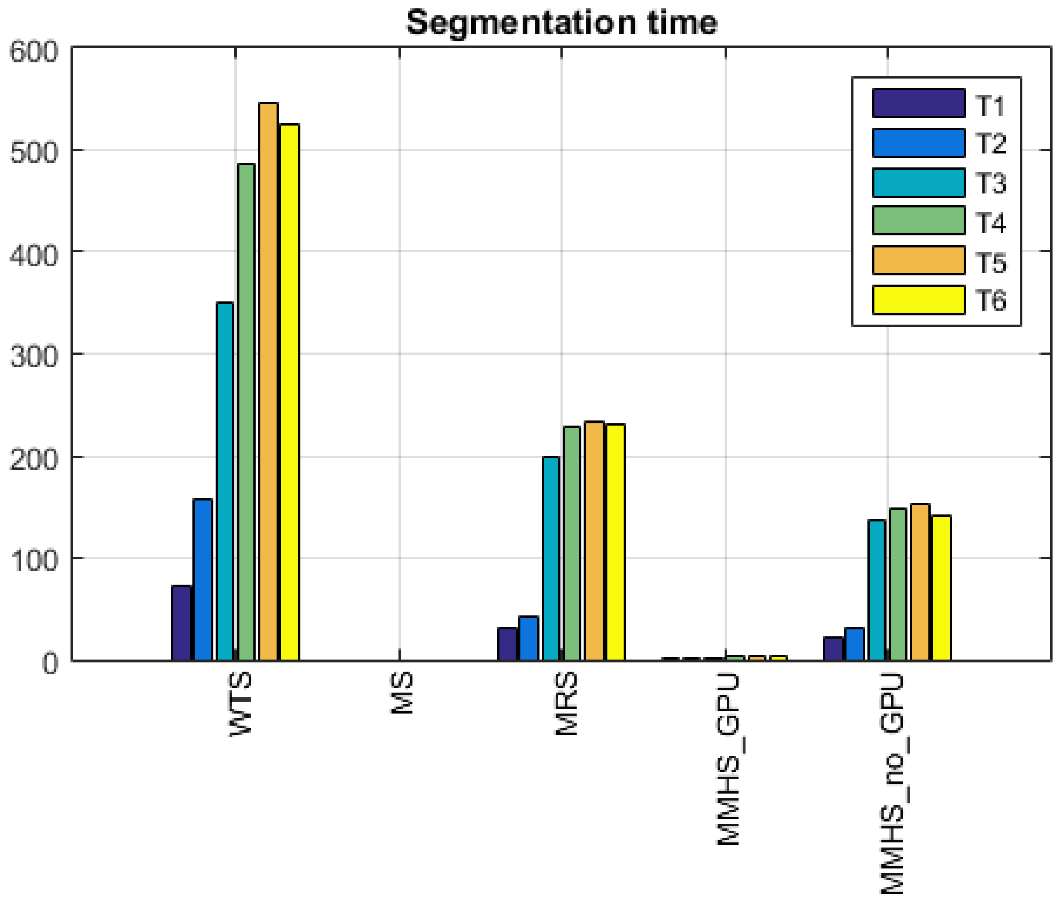
3.3.3. Segmentation Time and Mean Accuracy

The well-recognized segmentation algorithm is the MRS of eCognition. It takes about three minutes to segment a 6000 × 6000 remote sensing image once. To achieve the ideal segmentation result, it is necessary to repeat the segmentation of different scales more than 10 times. Thus, this process is very time consuming. Therefore, our algorithm is expected to greatly improve the segmentation efficiency of remote sensing images. This section presents an overall comparison of the MMHS segmentation time and average segmentation accuracy.

Since our algorithm uses GPU acceleration in the superpixel over-segmentation phase and superpixel feature calculation phase, we analyzed the segmentation time of MMHS without GPU and with GPU. At the same time, based on the above six image segmentation evaluation result, we also analyzed the mean segmentation accuracy of our algorithm. The implemented environments of WTS, MS, MRS and MMHS are introduced in Section 3. Our MMHS does not need to record the cycle arcs in a priority queue, so its computational complexity just depends on the local-oriented update of the graph model. If the number of merging iterations is n, then the complexity of LMM is O(hn), where h represents the complexity of updating the graph model at a merging iteration. As described in

Table 11. The segmentation time of different methods.

Test Image	Image Size	Segmentation Time (s)
		WTS	MS	MRS	MMHS with GPU	MMHS without GPU
T1	2324 × 2324	73	244	30.5	0.468	22
T2	2979 × 2979	156.7	374.2	43.2	0.874	31
T3	6000 × 6000	350.4	11,484	198	2.199	136.5
T4	6000 × 6000	486.88	17,721	228.6	2.570	149.3
T5	6000 × 6000	545.3	19,051	233.4	2.730	153.2
T6	6000 × 6000	524.9	18,545	230.1	2.670	140.8

and Figure 15, the segmentation times of MMHS with GPU and MMHS without GPU are both lower than those of others. It can be clearly seen that the MS algorithm is very slow and needs to be improved for HSR remote sensing images. In order to better compare other methods, we did not draw a histogram for MS. The WTS method averaged segmentation time was shown to be more than twice that of MRS. Our MMHS algorithm without GPU acceleration took, on average, 55 s less than MRS, while the GPU-accelerated version of MMHS reached the second level and the speed advantage was very obvious.

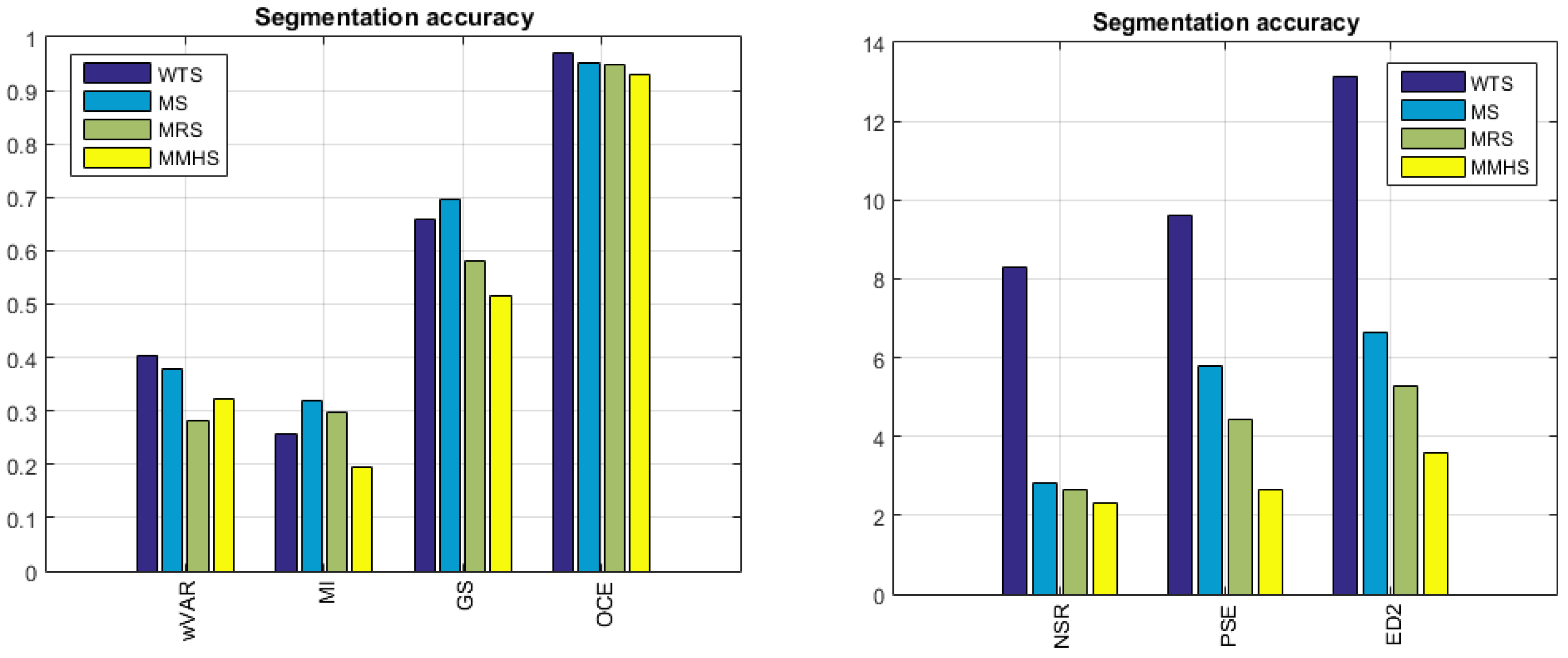
In addition to the advantages of time, our algorithm also showed good segmentation accuracy.

Table 12. The mean quantitative assessment results of T1–T6.

Method	Mean Segmentation Accuracy
	wVar	MI	GS	NSR	PSE	ED2	OCE
WT	0.4046	0.2558	0.6604	8.2736	9.6057	13.144	0.9701
MS	0.3775	0.3203	0.6977	2.8095	5.7826	6.6317	0.9512
MRS	0.2827	0.2973	0.5800	2.6505	4.4263	5.2778	0.9488
MMHS	0.3212	0.1946	0.5157	2.3012	2.6519	3.5839	0.9286

and Figure 16 show the average segmentation accuracy comparison results of the four algorithms. It can be seen that besides the wVAR index, our algorithm obtained the optimal segmentation accuracy. Compared with the wVAR index, our algorithm was lower than MRS, which is different from the local variance calculated by the sliding window in Woodcock and Strahler’s literature [46,47]. The wVAR is a global variance. In a further comparison of Table 2 and Table 3 the WTS and MS segmentation accuracy shows that if the image is severely over-segmentated, its wVar value will become smaller. Therefore, it is necessary to calculate the GS value combined with MI to further evaluate the segmentation accuracy. Of course, using the idea from the literature presented in reference [46,47] to improve the wVar indicator in GS may also be a good solution.

3.4. Sensitivity Analysis

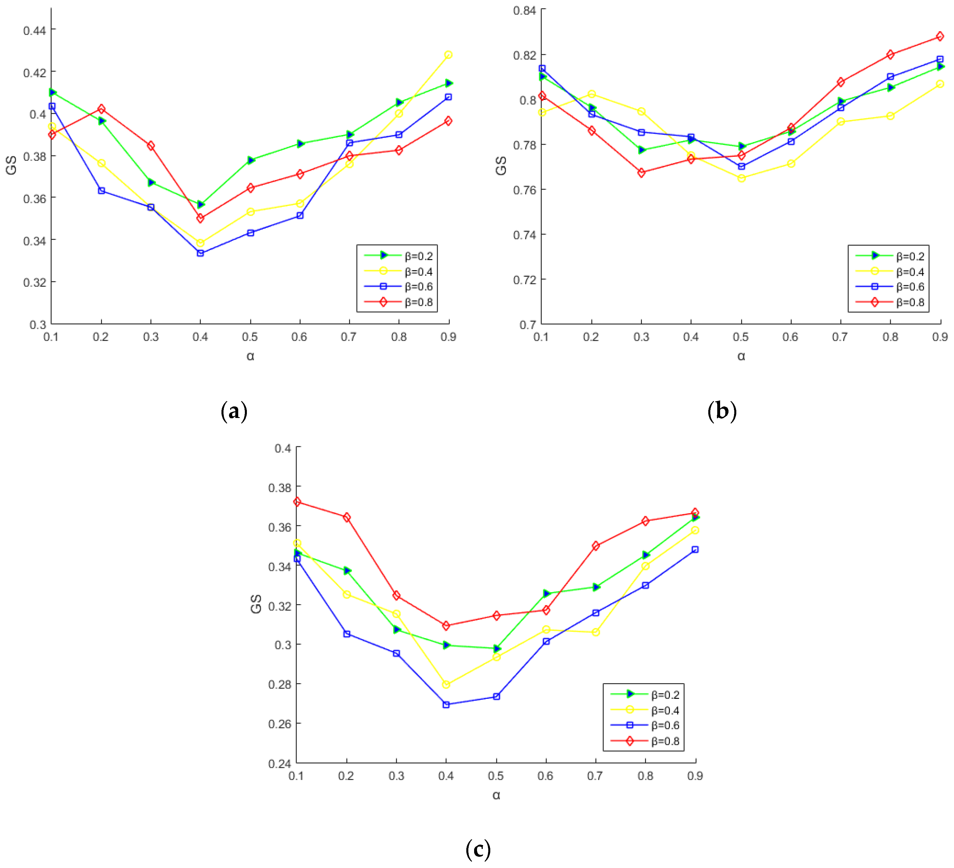
In this section, we present the analysis of the sensitivity of the weight parameters—color $\left(\alpha \right)$, texture $\left(\beta \right)$, boundary constraint parameters $\left({\sigma }_e\right)$—of our MMHS algorithm on the segmentation result accuracy. In essence, this is a process of selecting the texture, spectral, and boundary features in a balanced manner when facing different ground objects. We chose T1, T2, and T3, which represent three typical images of towns, cities and forests. The number of segments was set as 74, 105, and 109 for T1, T2, and T3, respectively. By adjusting α and β, the variation of the segmentation accuracy GS was calculated, and the corresponding graph was plotted.

As shown in Figure 17, the different curves in the three experimental graphs represent the changes in the non-supervised segmentation accuracy GS. The experiment texture weight parameters β were 0.2, 0.4, 0.6, and 0.8, respectively, when the color weight parameter α changed from 0 to 0.9, and the boundary constraint parameters $\left({\sigma }_e^2\right)$ were 0.4, 0.3, and $0.5$ for the T1, T2, and T3 images, respectively. Compared with the distribution of the curves in Figure 17a–c, they had similar trends. When the value of β was constant, the change of the GS value became smaller with the increase of α and then became larger. This shows that the segmentation accuracy of the algorithm is affected by the distribution of spectral and texture weights. For HSR images, the spectral information plays the most important role in most cases. At the initial stage, the HSR image is over-segmented, the range of each superpixel is small, and the spectral features are more stable and accurate than the texture features. So, for the influence of segmentation accuracy, the effects of the spectral features are more obvious. As the spectral feature weights increase, the segmentation accuracy gradually increases, and when the texture and spectral weights are optimally balanced, the segmentation accuracy GS reaches an optimal value. After that, when the spectral feature weights continue to increase, the influence of texture features begins to increase, and the weights of the texture and the spectrum become unbalanced. As a result, the segmentation accuracy gradually decreases. The optimal GS values of the three datasets for MMHS were 0.3333, 0.7648 and 0.2693, respectively. From Figure 17a,c, the T1 and T3 segmentation accuracies were best at α = 0.4 and β = 0.6. Figure 17b shows that when α = 0.5 and β = 0.4, the segmentation accuracy of T2 was optimal. In general, the variation range of the segmentation accuracy GS was about 0.15, which indicates that although the selection of feature weights affects the segmentation accuracy, the segmentation accuracy can still maintain good stability.

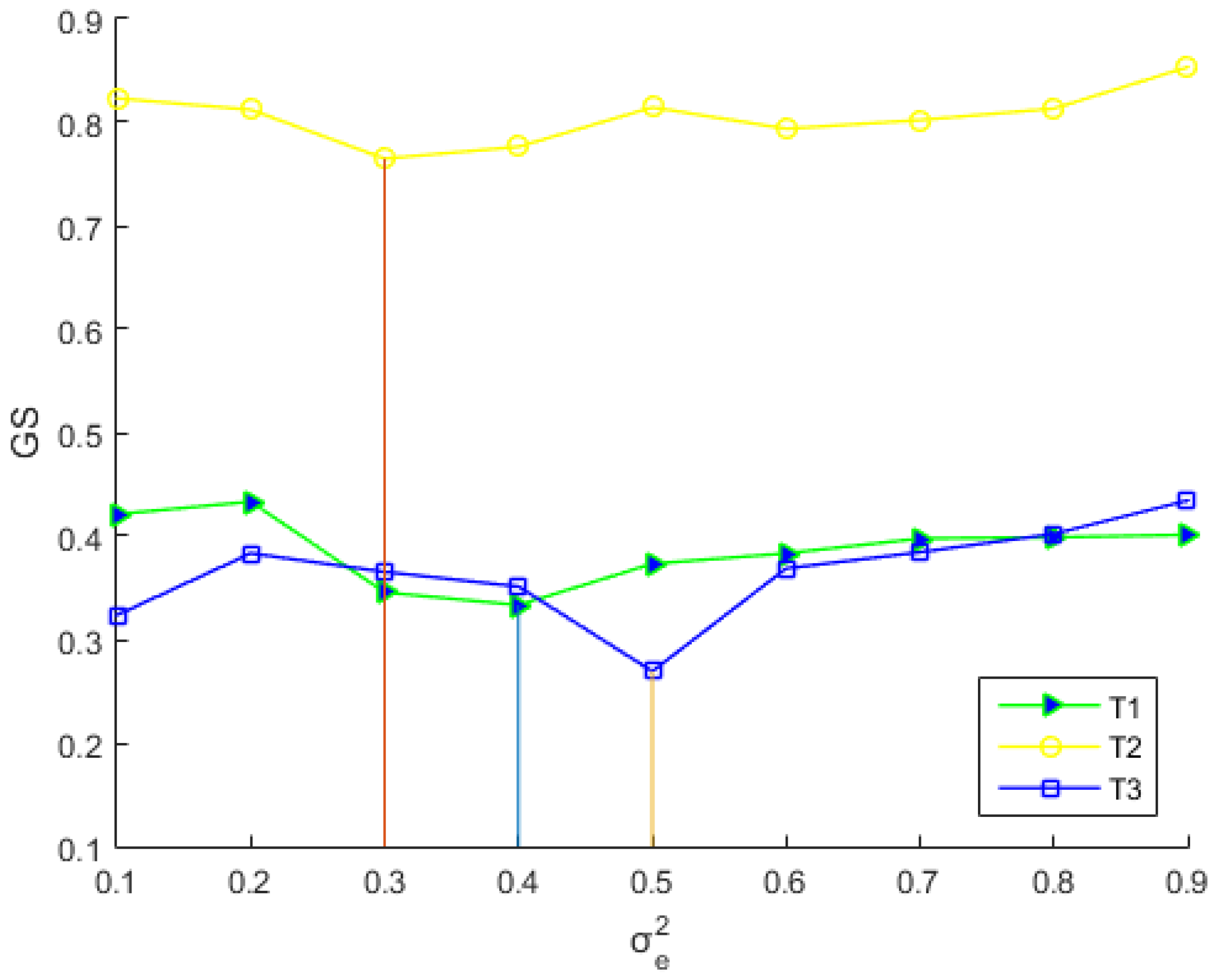
In order to analyze the impact of parameter ${\sigma }_e$ on the segmentation result accuracy, the parameter color $\left(\alpha \right)$ and texture $\left(\beta \right)$ were set as 0.4/0.5/0.4 and 0.6/0.4/0.6, and ${\sigma }_e^2$ was chosen from the region of {0.1, 0.2, …, 0.9} for the T1, T2, and T3 datasets, respectively. It can be observed from Figure 18 that the GS values of the three images firstly decreased and then increased. This demonstrates that the segmentation accuracy deteriorates when the boundary constraint $\left({\sigma }_e^2\right)$ value is too small or too large. When the boundary constraint is too small, even if the shared boundary is short, as long as the colors or textures of the two adjacent superpixels are sufficiently similar, they will be directly merged into a sub-region. Thus, it is easy to cause a jagged boundary phenomenon. On the other hand, if the boundary constraint is too large, it will prevent the merging of the ideal grouping area, resulting in over-segmentation. So, as can be seen, the boundary constraint $\left({\sigma }_e^2\right)$ can obviously improve the segmentation quality on these test areas. This is because, under equal conditions, merging priority is given to the couple of regions that share the longest boundary. For the T1, T2, and T3 test images, the optimal segmentation accuracies were obtained when the ${\sigma }_e^2$ was set to 0.4, 0.3, and $0.5$, respectively.

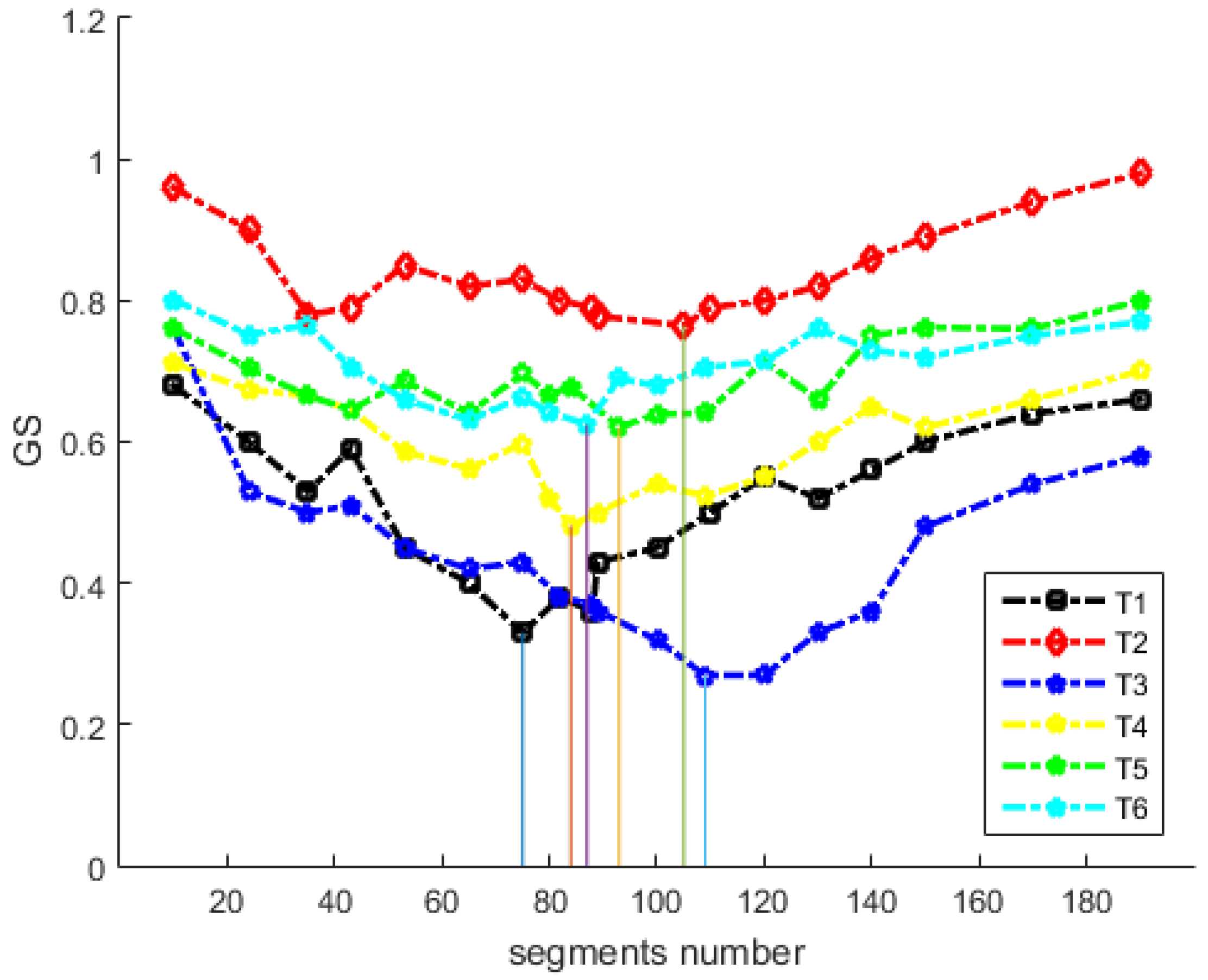
3.5. Effect of Superpixel Scale Selection

In this section, we present the analysis of the effect of segmentation scale selection and determined for the optimal number of segments. Woodcock and Strahler [47] proposed measuring the relationship of landscape features in different spatial resolutions using a n × n moving window. In this method, the mean value of the standard deviation (SD) of the spectral attributes within the window is calculated, which is the LV. Finally, the LV curve is formed to obtain the best image resolution [47]. The authors explain the mechanism as follows: if the spatial resolution is considerably finer than the objects in the scene, most of the measurements in the image will be highly correlated with their neighbor cells, and then, the likelihood of neighbors being similar decreases and the LV rises. Since reference [46] introduced these theories into digital images, the semivariogram method has been widely applied to scale modeling of remote sensing images [48]. The semivariogram can represent how a variable’s variance changes with different sampling intervals on one image, which can represent the degree or scale of spatial variability. Lucian et al. [49] improved the LV method to propose the estimation of scale parameter (ESP) tool. The solution consists of inspecting the indicator diagram of the local variance (LV) and the rate of change in LV (ROC-LV) produced using the ESP tool. It is a scale parameter estimation plug-in developed for eCognition software that calculates the local variance of homogeneous image objects using different scale parameters.

Different from the local variance used by ESP, our work attempted to use the global score (GS) which is calculated by adding the normalized weighted variance (wVar) and the normalized global Moran index (MI). The variance of the segmented region can reflect the relative degree of homogeneity of the region and is often chosen as the intra-segment goodness measure. wVar is a global calculation based on the area of the segmented region, which makes large segments have more impact on global homogeneity. Global Moran’s I is a spatial autocorrelation measure that can characterize the degree of similarity between an area and its neighbors and can be used as a good indicator of segmentation quality. Brian Johnson [38] chose it as the inter-segment global goodness measure in the calculation of the global score (GS). Low Moran’s I values indicate high inter-segment heterogeneity, which is desirable for image segmentation. So, in theory, a good segmentation result should have a low global score. The global score (GS) can reflect the intra- and inter-segment heterogeneity information to evaluate the optimal scale selection. At the same time, we selected the same datasets for this analysis. As illustrated in Figure 19, with an increase in the segmentation number, the resulting GS values firstly retain a downtrend, while when the value of GS reaches the lowest peak, it tends to increase for each dataset. This means that as the number of segments is too small or too large, segments tended to have much higher variance and became more similar to neighboring segments. The optimal segmentation number is the point at which this GS value reaches the lowest value and segments are, on average, most homogeneous internally and most different from their neighbors. Therefore, the optimal numbers of segmentation for the six datasets were 74, 105, 109, 84, 93, and 87, respectively. In further analyses, T1, T2, T3, T4, T5, and T6 represented three different regions of town, city and forest, respectively and the average GS value of the three was also very different. For urban area T2, the mean GS was the highest and T3 was the lowest. This may have been because study area T3 was a more homogeneous forest scene, in which the spectral values for the different types of land cover were quite similar. Image T2 was a more heterogeneous urban area, where different types of land cover have very different spectral characteristics. Therefore, in these more heterogeneous environments, variance and Moran’s I will likely continue to be at a high level, and we also combined the judgment of visual effects to determine the optimal value of the segmentation number.

4. Discussion

The novelty of this study is that we used gSLICr superpixels to decompose the complexity of HSR remote sensing data into perceptually meaningful uniform blocks, efficient multifeature similarity calculations, and multiscale LMM merger strategies. First, the MMHS method was shown to achieve near real-time efficiency. It has the potential to be a framework for real-time HSR remote sensing processing. Secondly, we fused diverse features in an effective manner which is an adjustable multifeature integration strategy to handle complex situations of HSR images. Thirdly, in MMHS, we were able to obtain multiscale hierarchical segmentation results. Our work attempted to use the intra- and inter-segment heterogeneity information to address the optimal scale problem.

Obviously, our method makes full use of spectral, texture, scale, local, global information, and these parameters can be adjusted for various objects. A comparison of pixel-based and superpixel-based segmentation revealed the fact that better segmentation accuracy can be achieved using superpixels instead of pixels. In terms of segmentation time, our algorithm was dozens of times faster than the traditional method. It showed significant advantages over the traditional algorithm and avoided the disadvantages of these methods. The segmentation result was described both in vector and raster format and established a better foundation for higher level image processing, such as pattern recognition and image classification. Our method can also be applied to other similar remote sensing applications. At the same time, it could be further improved, for example, it could integrate more features, including the size of superpixels and more simple and effective features. Overall, based on our design philosophy, this method can further improve his segmentation efficiency and accuracy.

Superpixels originate from computer vision applications. In remote sensing, superpixels greatly improve the processing efficiency of large-scale HSR remote sensing images. For example, GPU-based superpixel processing technology has great application prospects for real-time video processing applications of drones and commercial video satellites [50]. This is also the focus of our future research.

Of course, this paper found some problems in the evaluation of segmentation accuracy. There are many methods for image segmentation evaluation. However, the applicability and accuracy of these methods is another issue worth studying. Firstly, in order to be more objective, the segmentation methods should distinguish the calculation principles of the evaluation methods. Secondly, was found in our experiment that when the OCE is used to evaluate the segmentation result, even if the segmentation effect is good, the OCE value is still too large, which indicates that the sensitivity of OCE method in segmentation quality is not enough. Third, the optimal unsupervised GS quantitative evaluation value is obtained by normalizing the multiple segmentation results of each algorithm. The calculation of MI in the GS indicator is complicated, and it is necessary to deal with negative numbers. We believe that the above problems can be further improved so that the evaluation of remote sensing image segmentation is more fast, simple and effective. The calculation of ED2 is a good example. It uses the AssesSeg tool, a command line tool to quantify image segmentation quality [51], which allows easy and fast segmentation evaluation.

The optimal segmentation result of our algorithm in this paper was obtained by calculating the GS evaluation index and visually judging the segmentation results on different scales. The scale problem of HSR remote sensing image segmentation is an unavoidable one, so the disadvantage of our method is the determination of superpixel size and the optimal merging indexes. HSR image features are complex, and there are many changes in texture, spectrum, shape, and scale. The features in the superpixel area will be unified, and the small -cale boundary information will be discarded. The size of the superpixel determines the boundary accuracy in the subsequent segmentation. According to different objects features, the corresponding superpixel size for initial over-segmentation is selected. Although the NNG and LMM strategies guarantee efficient local optimization, the essence of the optimal combination index is the ideal value of the local and global optimal in the segmentation process. The question of how to obtain the best combination index in the segmentation results obtained in this paper will also be the focus of future research.

5. Conclusions

In this study, we presented an effective method, MMHS, for multiscale multifeature HSR imagery segmentation using three HSR remote sensing datasets, and we evaluated its performance by comparing three widely used state-of-the-art methods, which were analyzed based on supervised and unsupervised image segmentation evaluation methods. The first step of our algorithm is a fast up-bottom procedure that generates initial superpixels on modern GPUs. In the second step, diverse features are fused in an effective manner to calculate the similarity between superpixels. An NNG is constructed, and a bottom-up region merging algorithm is used based on the LMM principle to obtain the final segmentation. Compared with the traditional methods, the extensive experimental results showed that our algorithm has advantages in terms of both segmentation accuracy and computation time, regardless of quantitative criteria or visual judgment. To some extent, this method can be widely applied to HSR remote sensing data analysis and has the potential to be a framework for real-time processing.