Crop Classification in a Heterogeneous Arable Landscape Using Uncalibrated UAV Data


Abstract
1. Introduction
2. Material
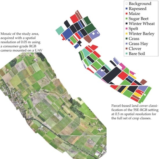
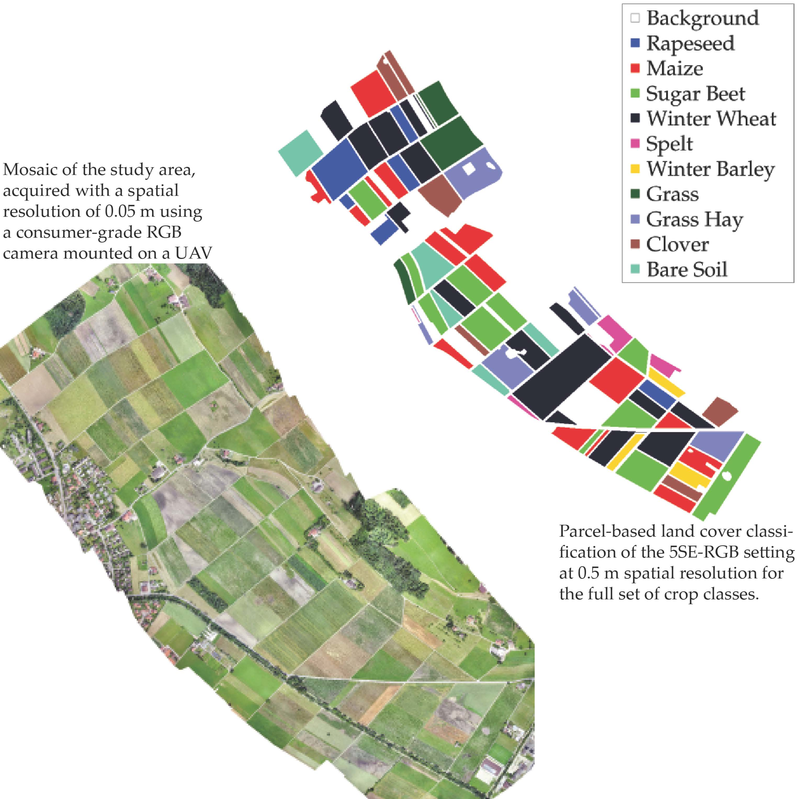
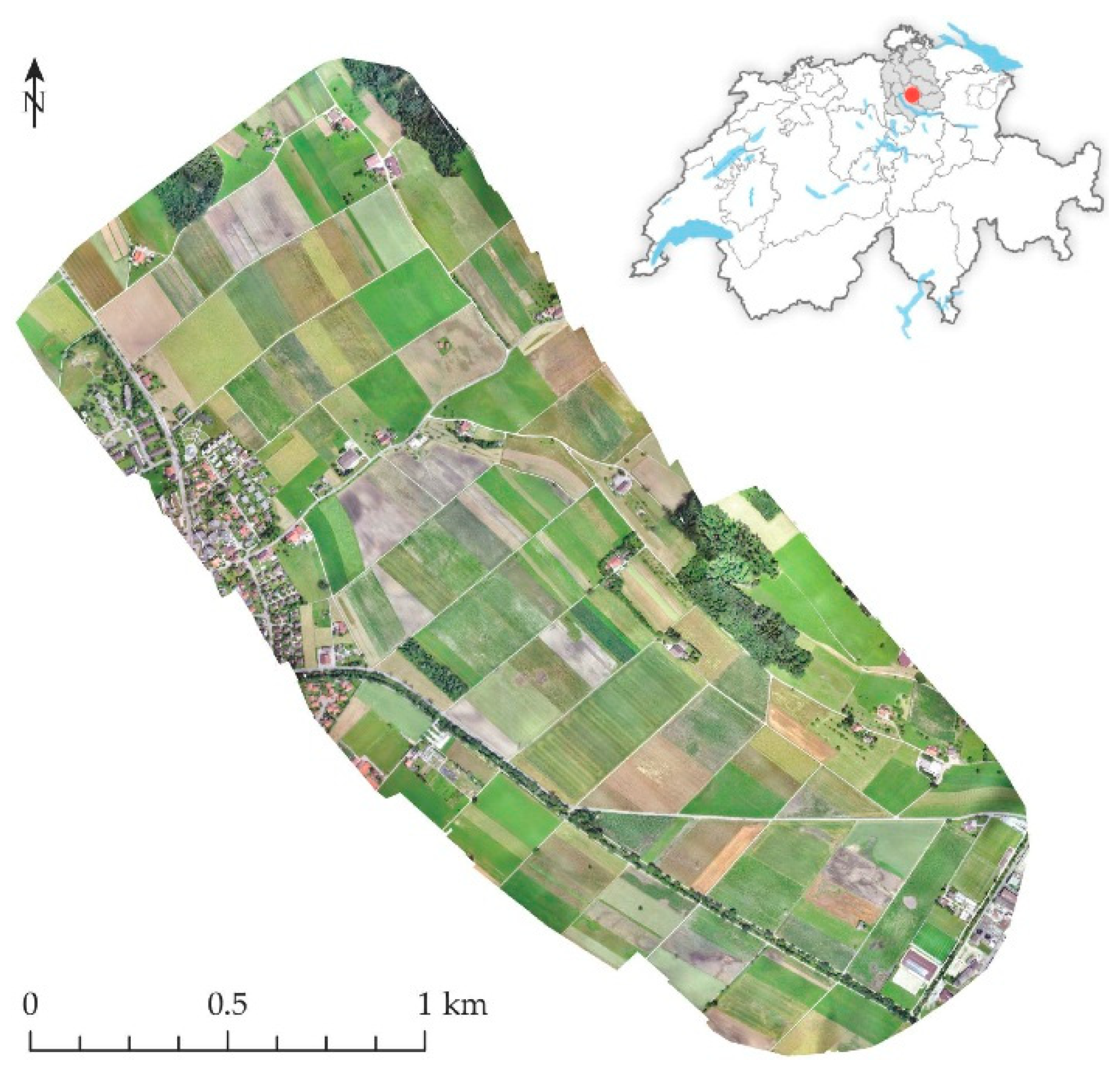
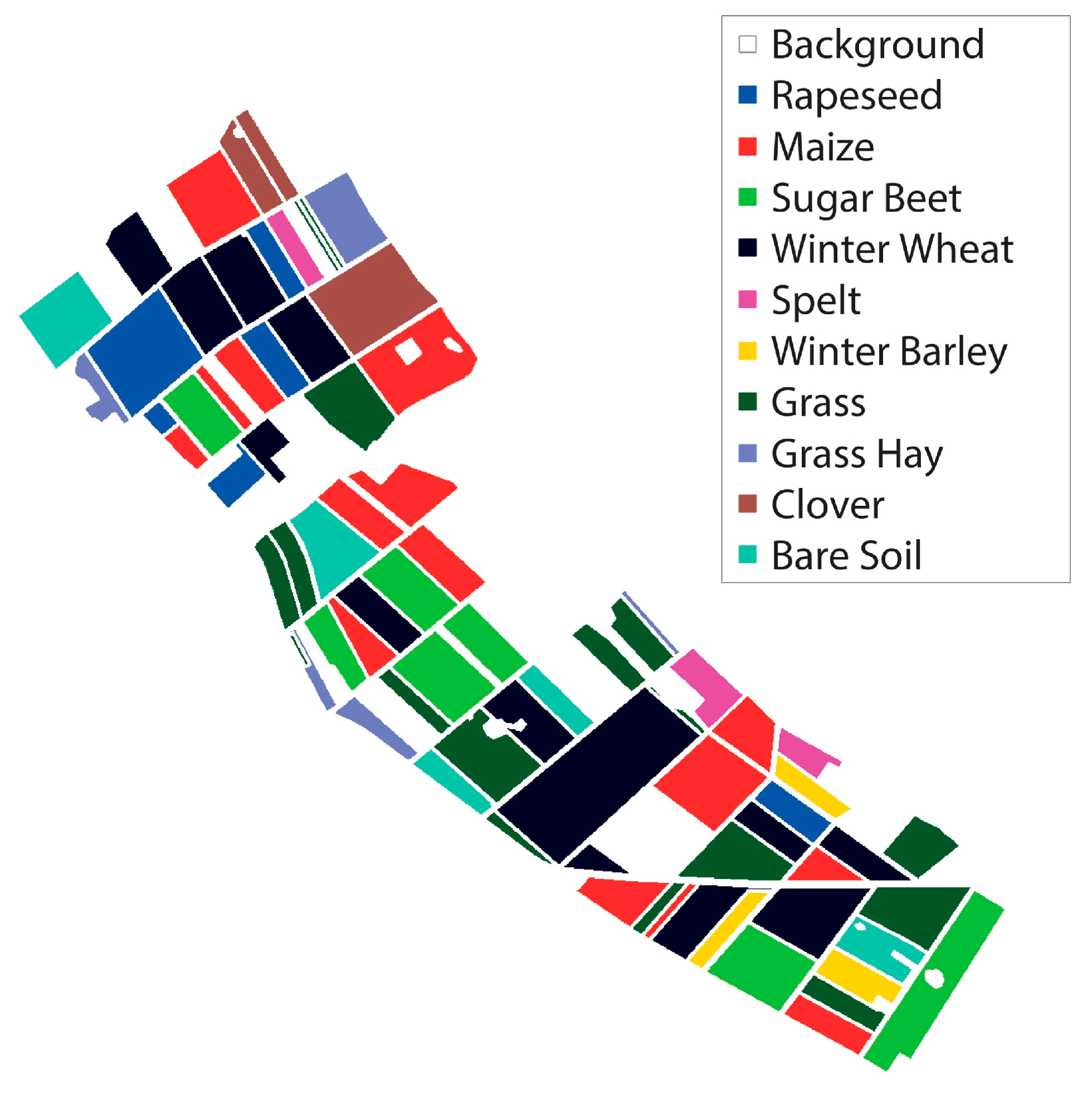
2.1. Study Area
2.2. Dataset
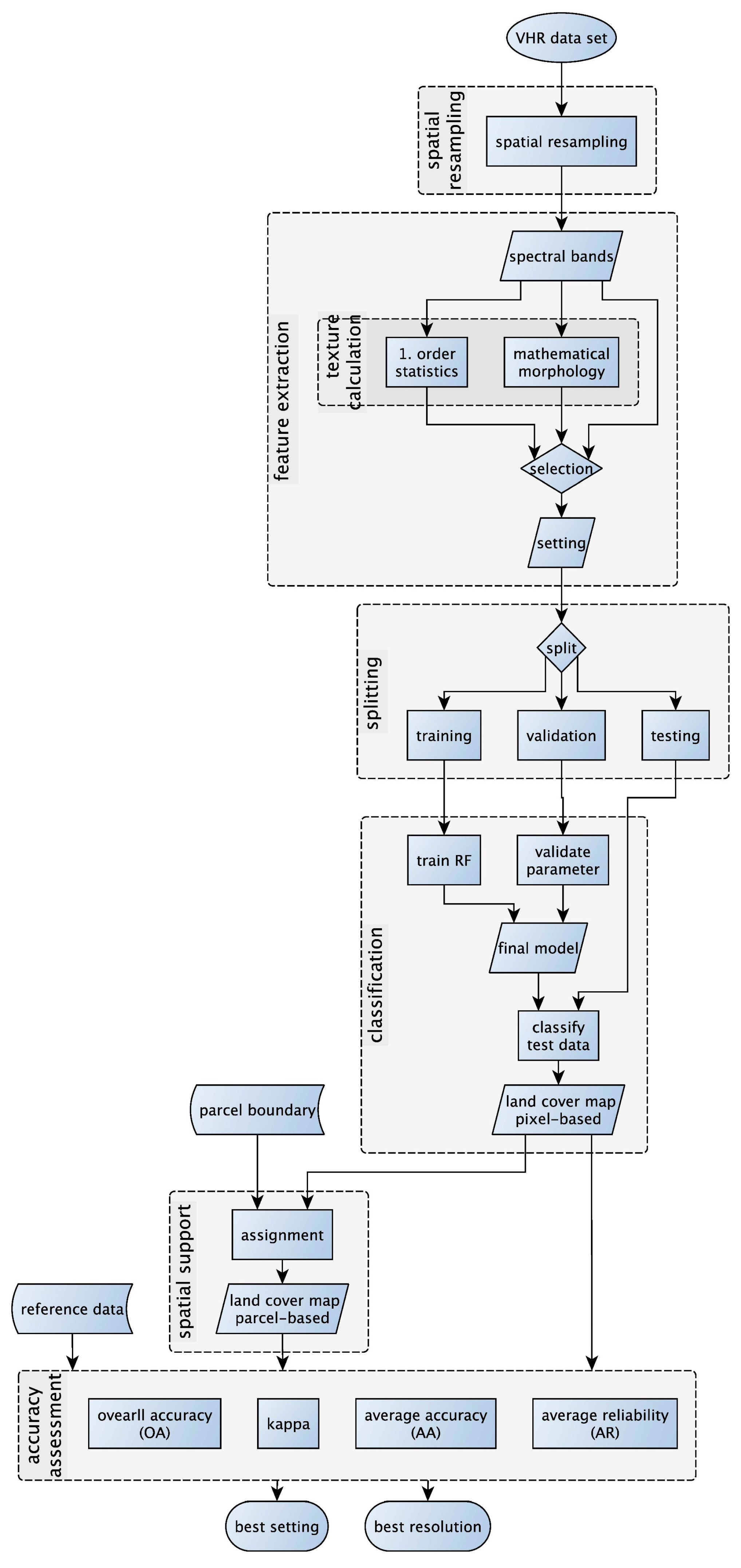
3. Method
3.1. Resampling
3.2. Feature Extraction
3.3. Data Splitting for Validation
3.4. Classification
3.5. Spatial Support
3.6. Accuracy Assessment
4. Results
4.1. Spatial Resampling
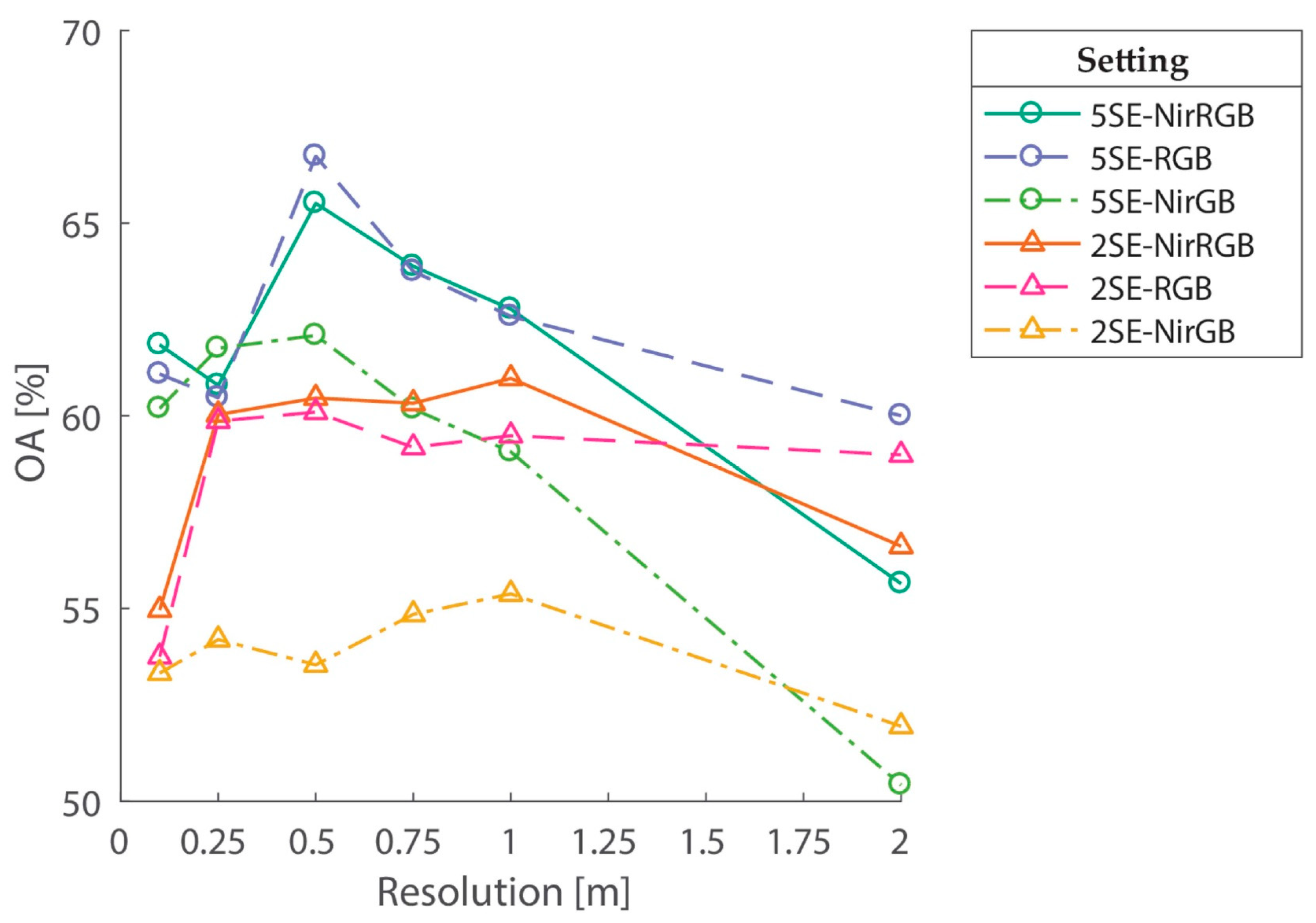
4.2. Spectral Resolution
4.3. Number of SE Sizes
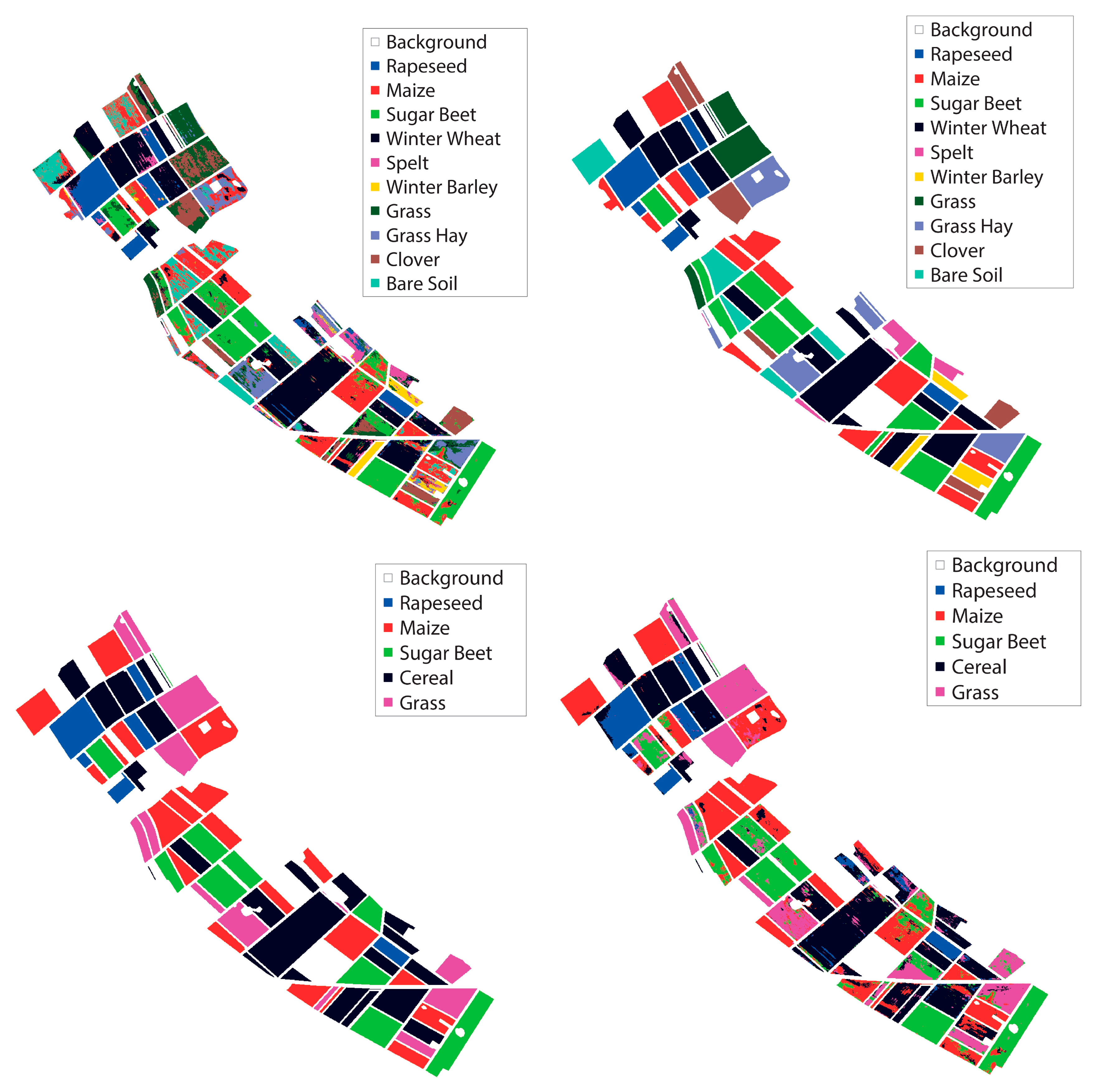
4.4. Number of Classes and Spatial Support
4.5. Class Specific Accuracy
5. Discussion
5.1. Influence of Spatial Resolution
5.2. Impact of Spectral Characteristics
5.3. Effect of Different SE sizes
5.4. Influence of Spatial Support
5.5. Considerations about Acquisition Date and Temporal Resolution
5.6. Comparison to Other Studies
5.7. Limitations of Our Method
6. Conclusions
Supplementary Materials
Author Contributions
Funding
Acknowledgments
Conflicts of Interest
References
- Rosenzweig, C.; Elliott, J.; Deryng, D.; Ruane, A.C.; Müller, C.; Arneth, A.; Boote, K.J.; Folberth, C.; Glotter, M.; Khabarov, N.; et al. Assessing agricultural risks of climate change in the 21st century in a global gridded crop model intercomparison. Proc. Natl. Acad. Sci. USA 2014, 111, 3268–3273. [Google Scholar] [CrossRef] [PubMed]
- Gerland, P.; Raftery, A.E.; Ševčíková, H.; Li, N.; Gu, D.; Spoorenberg, T.; Alkema, L.; Fosdick, B.K.; Chunn, J.; Lalic, N.; et al. World population stabilization unlikely this century. Science 2014, 346, 234–237. [Google Scholar] [CrossRef] [PubMed]
- Tilman, D.; Balzer, C.; Hill, J.; Befort, B.L. Global food demand and the sustainable intensification of agriculture. Proc. Natl. Acad. Sci. USA 2011, 108, 20260–20264. [Google Scholar] [CrossRef] [PubMed]
- Whitcraft, A.K.; Becker-Reshef, I.; Justice, C.O. A framework for defining spatially explicit earth observation requirements for a global agricultural monitoring initiative (GEOGLAM). Remote Sens. 2015, 7, 1461–1481. [Google Scholar] [CrossRef]
- Fuhrer, J.; Gregory, P.J. Climate Change Impact and Adaptation in Agricultural Systems; CABI: Wallingford, CT, USA, 2014; ISBN 9781780642895. [Google Scholar]
- Atzberger, C. Advances in Remote Sensing of Agriculture: Context Description, Existing Operational Monitoring Systems and Major Information Needs. Remote Sens. 2013, 5, 949–981. [Google Scholar] [CrossRef]
- Kastens, J.H.; Kastens, T.L.A.; Kastens, D.L.A.; Price, K.P.; Martinko, E.A.; Lee, R.Y. Image masking for crop yield forecasting using AVHRR NDVI time series imagery. Remote Sens. Environ. 2005, 99, 341–356. [Google Scholar] [CrossRef]
- Zhang, P.; Anderson, B.; Tan, B.; Huang, D.; Myneni, R. Potential monitoring of crop production using a satellite-based Climate-Variability Impact Index. Agric. For. Meteorol. 2005, 132, 344–358. [Google Scholar] [CrossRef]
- Mueller, N.D.; Gerber, J.S.; Johnston, M.; Ray, D.K.; Ramankutty, N.; Foley, J.A. Closing yield gaps through nutrient and water management. Nature 2012, 490, 254–257. [Google Scholar] [CrossRef] [PubMed]
- Verbesselt, J.; Hyndman, R.; Newnham, G.; Culvenor, D. Detecting trend and seasonal changes in satellite image time series. Remote Sens. Environ. 2010, 114, 106–115. [Google Scholar] [CrossRef]
- Rembold, F.; Atzberger, C.; Savin, I.; Rojas, O. Using low resolution satellite imagery for yield prediction and yield anomaly detection. Remote Sens. 2013, 5, 1704–1733. [Google Scholar] [CrossRef]
- Galford, G.L.; Mustard, J.F.; Melillo, J.; Gendrin, A.; Cerri, C.C.; Cerri, C.E.P. Wavelet analysis of MODIS time series to detect expansion and intensification of row-crop agriculture in Brazil. Remote Sens. Environ. 2008, 112, 576–587. [Google Scholar] [CrossRef]
- Wardlow, B.D.; Egbert, S.L.; Kastens, J.H. Analysis of time-series MODIS 250 m vegetation index data for crop classification in the U.S. Central Great Plains. Remote Sens. Environ. 2007, 108, 290–310. [Google Scholar] [CrossRef]
- Palchowdhuri, Y.; Valcarce-Diñeiro, R.; King, P.; Sanabria-Soto, M. Classification of multi-temporal spectral indices for crop type mapping: A case study in Coalville, UK. J. Agric. Sci. 2018, 156, 24–36. [Google Scholar] [CrossRef]
- Azar, R.; Villa, P.; Stroppiana, D.; Crema, A.; Boschetti, M.; Brivio, P.A. Assessing in-season crop classification performance using satellite data: A test case in Northern Italy. Eur. J. Remote Sens. 2016, 49, 361–380. [Google Scholar] [CrossRef]
- Ozdarici-Ok, A.; Ok, A.; Schindler, K. Mapping of Agricultural Crops from Single High-Resolution Multispectral Images--Data-Driven Smoothing vs. Parcel-Based Smoothing. Remote Sens. 2015, 7, 5611–5638. [Google Scholar] [CrossRef]
- Inglada, J.; Arias, M.; Tardy, B.; Hagolle, O.; Valero, S.; Morin, D.; Dedieu, G.; Sepulcre, G.; Bontemps, S.; Defourny, P.; et al. Assessment of an operational system for crop type map production using high temporal and spatial resolution satellite optical imagery. Remote Sens. 2015, 7, 12356–12379. [Google Scholar] [CrossRef]
- Immitzer, M.; Vuolo, F.; Atzberger, C. First experience with Sentinel-2 data for crop and tree species classifications in central Europe. Remote Sens. 2016, 8, 166. [Google Scholar] [CrossRef]
- Shi, Y.; Thomasson, J.A.; Murray, S.C.; Pugh, N.A.; Rooney, W.L.; Shafian, S.; Rajan, N.; Rouze, G.; Morgan, C.L.S.; Neely, H.L.; et al. Unmanned Aerial Vehicles for High-Throughput Phenotyping and Agronomic Research. PLoS ONE 2016, 11, e0159781. [Google Scholar] [CrossRef] [PubMed]
- Tattaris, M.; Reynolds, M.P.; Chapman, S.C. A Direct Comparison of Remote Sensing Approaches for High-Throughput Phenotyping in Plant Breeding. Front. Plant Sci. 2016, 7, 1131. [Google Scholar] [CrossRef] [PubMed]
- Holman, F.H.; Riche, A.B.; Michalski, A.; Castle, M.; Wooster, M.J.; Hawkesford, M.J. High Throughput Field Phenotyping of Wheat Plant Height and Growth Rate in Field Plot Trials Using UAV Based Remote Sensing. Remote Sens. 2016, 8, 1031. [Google Scholar] [CrossRef]
- Fuhrer, J.; Tendall, D.; Klein, T.; Lehmann, N.; Holzkämper, A. Water Demand in Swiss Agriculture—Sustainable Adaptive Options for Land and Water Management to Mitigate Impacts of Climate Change; Art-Schriftenreihe: Ettenhausen, Switzerland, 2013; Volume 59, Available online: https://www.agroscope.admin.ch/agroscope/de/home/publikationen/suchen/reihen-bis-2013/art-schriftenreihe.html (accessed on 14 August 2018).
- De Wit, A.J.W.; Clevers, J.G.P.W. Efficiency and accuracy of per-field classification for operational crop mapping. Int. J. Remote Sens. 2004, 25, 4091–4112. [Google Scholar] [CrossRef]
- Waldhoff, G.; Lussem, U.; Bareth, G. Multi-Data Approach for remote sensing-based regional crop rotation mapping: A case study for the Rur catchment, Germany. Int. J. Appl. Earth Obs. Geoinf. 2017, 61, 55–69. [Google Scholar] [CrossRef]
- Long, T.B.; Blok, V.; Coninx, I. Barriers to the adoption and diffusion of technological innovations for climate-smart agriculture in Europe: Evidence from the Netherlands, France, Switzerland and Italy. J. Clean. Prod. 2016, 112, 9–21. [Google Scholar] [CrossRef]
- Swiss Federal Office for Agriculture (FOAG). Swiss Agricultural Policy; FOAG: Berne, Switzerland, 2004; Available online: https://www.cbd.int/financial/pes/swiss-pesagriculturalpolicy.pdf (accessed on 14 August 2018).
- Benton, T.G.; Vickery, J.A.; Wilson, J.D. Farmland biodiversity: Is habitat heterogeneity the key? Trends Ecol. Evol. 2003, 18, 182–188. [Google Scholar] [CrossRef]
- Bundesrat, D.S. Verordnung über die Direktzahlungen an die Landwirtschaft. 2017, Volume 2013, pp. 1–152. Available online: https://www.admin.ch/opc/de/classified-compilation/20130216/index.html (accessed on 14 August 2018).
- Akademien der Wissenschaften Schweiz Brennpunkt Klima Schweiz. Grundlagen, Folgen, Perspektiven; Swiss Academies Reports; 2016; Volume 11, pp. 1–128. Available online: http://www.akademien-schweiz.ch (accessed on 14 August 2018).
- Vuolo, F.; Neugebauer, N.; Bolognesi, S.; Atzberger, C.; D’Urso, G. Estimation of Leaf Area Index Using DEIMOS-1 Data: Application and Transferability of a Semi-Empirical Relationship between two Agricultural Areas. Remote Sens. 2013, 5, 1274–1291. [Google Scholar] [CrossRef]
- Laliberte, A.S.; Rango, A. Texture and Scale in Object-Based Analysis of Subdecimeter Resolution Unmanned Aerial Vehicle (UAV) Imagery. IEEE Trans. Geosci. Remote Sens. 2009, 47, 761–770. [Google Scholar] [CrossRef]
- Marcos, D.; Volpi, M.; Kellenberger, B.; Tuia, D. Land cover mapping at very high resolution with rotation equivariant CNNs: Towards small yet accurate models. ISPRS J. Photogramm. Remote Sens. 2018, in press. [Google Scholar] [CrossRef]
- Whitehead, K.; Hugenholtz, C.H.; Myshak, S.; Brown, O.; LeClair, A.; Tamminga, A.; Barchyn, T.E.; Moorman, B.; Eaton, B. Remote sensing of the environment with small unmanned aircraft systems (UASs), Part 1: A review of progress and challenges. J. Unmanned Veh. Syst. 2014, 2, 69–85. [Google Scholar] [CrossRef]
- Khatami, R.; Mountrakis, G.; Stehman, S.V. A meta-analysis of remote sensing research on supervised pixel-based land-cover image classification processes: General guidelines for practitioners and future research. Remote Sens. Environ. 2016, 177, 89–100. [Google Scholar] [CrossRef]
- Zhang, H.; Li, Q.; Liu, J.; Shang, J.; Du, X.; McNairn, H.; Champagne, C.; Dong, T.; Liu, M. Image Classification Using RapidEye Data: Integration of Spectral and Textual Features in a Random Forest Classifier. IEEE J. Sel. Top. Appl. Earth Obs. Remote Sens. 2017, 10, 5334–5349. [Google Scholar] [CrossRef]
- Topaloglou, C.A.; Mylonas, S.K.; Stavrakoudis, D.G.; Mastorocostas, P.A.; Theocharis, J.B. Accurate crop classification using hierarchical genetic fuzzy rule-based systems. In Proceedings of the SPIE— Remote Sensing for Agriculture, Ecosystems, and Hydrology, Amsterdam, The Netherlands, 22–23 September 2014; Volume 9239. [Google Scholar]
- Helmholz, P.; Rottensteiner, F.; Heipke, C. Semi-automatic verification of cropland and grassland using very high resolution mono-temporal satellite images. ISPRS J. Photogramm. Remote Sens. 2014, 97, 204–218. [Google Scholar] [CrossRef]
- Debats, S.R.; Luo, D.; Estes, L.D.; Fuchs, T.J.; Caylor, K.K. A generalized computer vision approach to mapping crop fields in heterogeneous agricultural landscapes. Remote Sens. Environ. 2016, 179, 210–221. [Google Scholar] [CrossRef]
- Atkinson, P.M. Selecting the spatial resolution of airborne MSS imagery for small-scale agricultural mapping. Int. J. Remote Sens. 1997, 18, 1903–1917. [Google Scholar] [CrossRef]
- Pajares, G. Overview and Current Status of Remote Sensing Applications Based on Unmanned Aerial Vehicles (UAVs). Photogramm. Eng. Remote Sens. 2015, 81, 281–330. [Google Scholar] [CrossRef]
- Shahbazi, M.; Théau, J.; Ménard, P. Recent applications of unmanned aerial imagery in natural resource management. GISci. Remote Sens. 2014, 51, 339–365. [Google Scholar] [CrossRef]
- Ahmed, O.S.; Shemrock, A.; Chabot, D.; Dillon, C.; Williams, G.; Wasson, R.; Franklin, S.E. Hierarchical land cover and vegetation classification using multispectral data acquired from an unmanned aerial vehicle. Int. J. Remote Sens. 2017, 38, 2037–2052. [Google Scholar] [CrossRef]
- Colomina, I.; Molina, P. Unmanned aerial systems for photogrammetry and remote sensing: A review. ISPRS J. Photogramm. Remote Sens. 2014, 92, 79–97. [Google Scholar] [CrossRef]
- Hugenholtz, C.H.; Moorman, B.J.; Riddell, K.; Whitehead, K. Small unmanned aircraft systems for remote sensing and Earth science research. Eos Trans. Am. Geophys. Union 2012, 93, 236. [Google Scholar] [CrossRef]
- Whitehead, K.; Hugenholtz, C.H.; Myshak, S.; Brown, O.; LeClair, A.; Tamminga, A.; Barchyn, T.E.; Moorman, B.; Eaton, B. Remote sensing of the environment with small unmanned aircraft systems (UASs), Part 2: Scientific and commercial applications 1. J. Unmanned Veh. Syst. 2014, 2, 86–102. [Google Scholar] [CrossRef]
- Stöcker, C.; Bennett, R.; Nex, F.; Gerke, M.; Zevenbergen, J. Review of the Current State of UAV Regulations. Remote Sens. 2017, 9, 459. [Google Scholar] [CrossRef]
- Kelcey, J.; Lucieer, A. Sensor correction and radiometric calibration of a 6-band multispectral imaging sensor for UAV remote sensing. In Proceedings of the 12th Congress of the International Society for Photogrammetry and Remote Sensing, Melbourne, Australia, 25 August–1 September 2012; Volume 39, pp. 393–398. [Google Scholar]
- Lu, B.; He, Y. Species classification using Unmanned Aerial Vehicle (UAV)-acquired high spatial resolution imagery in a heterogeneous grassland. ISPRS J. Photogramm. Remote Sens. 2017, 128, 73–85. [Google Scholar] [CrossRef]
- Hueni, A.; Damm, A.; Kneubuehler, M.; Schläpfer, D.; Schaepman, M.E. Field and Airborne Spectroscopy Cross Validation—Some Considerations. IEEE J. Sel. Top. Appl. Earth Obs. Remote Sens. 2017, 10, 1117–1135. [Google Scholar] [CrossRef]
- Del Pozo, S.; Rodríguez-Gonzálvez, P.; Hernández-López, D.; Felipe-García, B. Vicarious Radiometric Calibration of a Multispectral Camera on Board an Unmanned Aerial System. Remote Sens. 2014, 6, 1918–1937. [Google Scholar] [CrossRef]
- Breiman, L. Random Forests. Mach. Learn. 2001, 45, 5–32. [Google Scholar] [CrossRef]
- MeteoSwiss Climate Normals Zürich/Fluntern Climate Normals Zürich/Fluntern. Available online: http://www.meteoswiss.admin.ch/product/output/climate-data/climate-diagrams-normal-values-station-processing/SMA/climsheet_SMA_np8110_e.pdf (accessed on 19 March 2018).
- Diek, S.; Schaepman, M.; de Jong, R. Creating Multi-Temporal Composites of Airborne Imaging Spectroscopy Data in Support of Digital Soil Mapping. Remote Sens. 2016, 8, 906. [Google Scholar] [CrossRef]
- Meier, U. Entwicklungsstadien mono-und dikotyler Pflanzen. Die erweiterte BBCH Monogr. 2001, 2. Available online: http://www.agrometeo.ch/sites/default/files/u10/bbch-skala_deutsch.pdf (accessed on 14 August 2018).
- Fernández-Delgado, M.; Cernadas, E.; Barro, S.; Amorim, D. Do we Need Hundreds of Classifiers to Solve Real World Classification Problems? J. Mach. Learn. Res. 2014, 15, 3133–3181. [Google Scholar]
- Fauvel, M.; Tarabalka, Y.; Benediktsson, J.A.; Chanussot, J.; Tilton, J.C. Advances in Spectral-Spatial Classification of Hyperspectral Images. Proc. IEEE 2013, 101, 652–675. [Google Scholar] [CrossRef]
- Tuia, D.; Pacifici, F.; Kanevski, M.; Emery, W.J. Classification of Very High Spatial Resolution Imagery Using Mathematical Morphology and Support Vector Machines. IEEE Trans. Geosci. Remote Sens. 2009, 47, 3866–3879. [Google Scholar] [CrossRef]
- Vincent, L. Morphological Grayscale Reconstruction in Image Analysis: Applications and Efficient Algorithms. IEEE Trans. Image Process. 1993, 2, 176–201. [Google Scholar] [CrossRef] [PubMed]
- Soille, P. Morphological Image Analysis; Springer: Berlin/Heidelberg, Germany, 2004; ISBN 978-3-642-07696-1. [Google Scholar]
- Ferro, C.J.S.; Warner, T.A. Scale and texture in digital image classification. Photogramm. Eng. Remote Sens. 2002, 68, 51–63. [Google Scholar]
- Lyons, M.B.; Keith, D.A.; Phinn, S.R.; Mason, T.J.; Elith, J. A comparison of resampling methods for remote sensing classification and accuracy assessment. Remote Sens. Environ. 2018, 208, 145–153. [Google Scholar] [CrossRef]
- Congalton, R. Assessing the Accuracy of Remotely Sensed Data; Mapping Science; CRC Press: Boca Raton, FL, USA, 2008; ISBN 978-1-4200-5512-2. [Google Scholar]
- Cohen, J. Weighted kappa: Nominal scale agreement provision for scaled disagreement or partial credit. Psychol. Bull. 1968, 70, 213–220. [Google Scholar] [CrossRef] [PubMed]
- Norman, J.; Welles, J. Radiative transfer in an array of canopies. Agron. J. 1983, 75, 481–488. [Google Scholar] [CrossRef]
- Flénet, F.; Kiniry, J.R.; Board, J.E.; Westgate, M.E.; Reicosky, D.A. Row spacing effects on light extinction coefficiencts of corn, sorghum, soybena, and sunflower. Agron. J. 1996, 88, 185–190. [Google Scholar] [CrossRef]
- Seginer, I.; Ioslovich, I. Optimal spacing and cultivation intensity for an industrialized crop production system. Agric. Syst. 1999, 62, 143–157. [Google Scholar] [CrossRef]
- Tokarczyk, P.; Wegner, J.D.; Walk, S.; Schindler, K. Features, Color Spaces, and Boosting: New Insights on Semantic Classification of Remote Sensing Images. IEEE Trans. Geosci. Remote Sens. 2015, 53, 280–295. [Google Scholar] [CrossRef]
- Wu, M.; Yang, C.; Song, X.; Hoffmann, W.C.; Huang, W.; Niu, Z.; Wang, C.; Li, W. Evaluation of orthomosics and digital surface models derived from aerial imagery for crop type mapping. Remote Sens. 2017, 9, 239. [Google Scholar] [CrossRef]
- Zhang, J.; Yang, C.; Song, H.; Hoffmann, W.C.; Zhang, D.; Zhang, G. Evaluation of an Airborne Remote Sensing Platform Consisting of Two Consumer-Grade Cameras for Crop Identification. Remote Sens. 2016, 8, 257. [Google Scholar] [CrossRef]
- Zhang, J.; Yang, C.; Zhao, B.; Song, H.; Hoffmann, W.C.; Shi, Y.; Zhang, D.; Zhang, G. Crop classification and LAI estimation using original and resolution-reduced images from two consumer-grade cameras. Remote Sens. 2017, 9, 2054. [Google Scholar] [CrossRef]


| Crop Class | Total Area (ha) | Number of Fields | Spacing | Phenology (BBCH) | ||
|---|---|---|---|---|---|---|
| Full Set | Merged Set | Within-Row (cm) | Row (cm) | |||
| Maize | Maize | 19.6 | 15 | 14-16 | 75 | 0–33 |
| Bare Soil | 7.4 | 5 | - | - | - | |
| Sugar Beet | Sugar Beet | 14.1 | 7 | 16 | 50 | 39 |
| Winter Wheat | Cereals | 24.4 | 13 | 5 | 14–15 | 75 |
| Spelt | 2.6 | 3 | 5 | 14–15 | 75 | |
| Winter Barley | 2.5 | 3 | 5 | 14–15 | 99 | |
| Grassland | Grassland | 15.0 | 17 | - | - | - |
| Clover | 5.4 | 3 | - | 10.5 | - | |
| Grass Hay | Excluded | 3.6 | 5 | - | - | - |
| Rapeseed | Rapeseed | 7.6 | 6 | 10 | 30 | 80 |
| Name | Formula |
|---|---|
| Dilatation | [εBf]x = minb ∈ Bf (x + b) |
| Erosion | [δBf]x = maxb ∈ Bf (x + b) |
| Opening | ΓBf = δB∘εB(f) |
| Closing | ϕBf = εB∘δB(f) |
| Opening by top hat | OTH = f − γBf |
| Closing by top hat | CTH = ϕBf − f |
| Opening by reconstruction | γR(n) = Rfδ[εnf] |
| Closing by reconstruction | ϕR(n) = Rfε[δn(f)] |
| Opening by reconstruction top hat | ORTH = f − γRn(f) |
| Closing by reconstruction top hat | CRTH = ϕRnf − f |
| Setting | Spectral Bands | SE Sizes (Diameter (Pixel)) |
|---|---|---|
| 5SE-NirRGB | NIR-R-G-B | 5SE (3, 5, 9, 13, 29) |
| 5SE-RGB | R-G-B | 5SE (3, 5, 9, 13, 29) |
| 5SE-NirGB | NIR-G-B | 5SE (3, 5, 9, 13, 29) |
| 2SE-NirRGB | NIR-R-G-B | 2SE (3, 5) |
| 2SE-RGB | R-G-B | 2SE (3, 5) |
| 2SE-NirGB | NIR-G-B | 2SE (3, 5) |
| Resolution (m) | Pixel-Based | Parcel-Based | ||
|---|---|---|---|---|
| Full Set | Merged Set | Full Set | Merged Set | |
| 0.1 | 61.1 | 80.2 | 76.1 | 94.7 |
| 0.25 | 60.5 | 86.5 | 69.9 | 96.7 |
| 0.5 | 66.7 | 86.3 | 74.0 | 94.6 |
| 0.75 | 63.7 | 86.5 | 65.7 | 96.2 |
| 1 | 62.6 | 86.0 | 61.9 | 94.3 |
| 2 | 60.0 | 82.7 | 67.8 | 92.2 |
| Settings | Pixel-Based | Parcel-Based | ||
|---|---|---|---|---|
| Full Set | Merged Set | Full Set | Merged Set | |
| 2SE-NirGB | 53.5 | 72.4 | 68.0 | 79.4 |
| 2SE-NirRGB | 60.5 | 77.1 | 75.6 | 83.5 |
| 2SE-RGB | 60.1 | 81.5 | 65.0 | 92.6 |
| 5SE-NirGB | 62.1 | 79.8 | 73.0 | 93.0 |
| 5SE-NirRGB | 65.5 | 83.5 | 76.7 | 95.0 |
| 5SE-RGB | 66.7 | 86.3 | 74.0 | 94.6 |
© 2018 by the authors. Licensee MDPI, Basel, Switzerland. This article is an open access article distributed under the terms and conditions of the Creative Commons Attribution (CC BY) license (http://creativecommons.org/licenses/by/4.0/).
Share and Cite
Böhler, J.E.; Schaepman, M.E.; Kneubühler, M. Crop Classification in a Heterogeneous Arable Landscape Using Uncalibrated UAV Data. Remote Sens. 2018, 10, 1282. https://doi.org/10.3390/rs10081282
Böhler JE, Schaepman ME, Kneubühler M. Crop Classification in a Heterogeneous Arable Landscape Using Uncalibrated UAV Data. Remote Sensing. 2018; 10(8):1282. https://doi.org/10.3390/rs10081282
Chicago/Turabian StyleBöhler, Jonas E., Michael E. Schaepman, and Mathias Kneubühler. 2018. "Crop Classification in a Heterogeneous Arable Landscape Using Uncalibrated UAV Data" Remote Sensing 10, no. 8: 1282. https://doi.org/10.3390/rs10081282
APA StyleBöhler, J. E., Schaepman, M. E., & Kneubühler, M. (2018). Crop Classification in a Heterogeneous Arable Landscape Using Uncalibrated UAV Data. Remote Sensing, 10(8), 1282. https://doi.org/10.3390/rs10081282