Article

Automated Cobble Mapping of a Mixed Sand-Cobble Beach Using a Mobile LiDAR System

Scripps Institution of Oceanography, University of California, San Diego, 9500 Gilman Dr., La Jolla, CA 92093, USA
*
Author to whom correspondence should be addressed.
Remote Sens. 2018, 10(8), 1253; https://doi.org/10.3390/rs10081253
Submission received: 22 June 2018 / Revised: 22 July 2018 / Accepted: 2 August 2018 / Published: 9 August 2018
(This article belongs to the Section Remote Sensing in Geology, Geomorphology and Hydrology)

Abstract

:
Cobbles (64–256 mm) are found on beaches throughout the world, influence beach morphology, and can provide shoreline stability. Detailed, frequent, and spatially large-scale quantitative cobble observations at beaches are vital toward a better understanding of sand-cobble beach systems. This study used a truck-mounted mobile terrestrial LiDAR system and a raster-based classification approach to map cobbles automatically. Rasters of LiDAR intensity, intensity deviation, topographic roughness, and slope were utilized for cobble classification. Four machine learning techniques including maximum likelihood, decision tree, support vector machine, and k-nearest neighbors were tested on five raster resolutions ranging from 5–50 cm. The cobble mapping capability varied depending on pixel size, classification technique, surface cobble density, and beach setting. The best performer was a maximum likelihood classification using 20 cm raster resolution. Compared to manual mapping at 15 control sites (size ranging from a few to several hundred square meters), automated mapping errors were <12% (best fit line). This method mapped the spatial location of dense cobble regions more accurately compared to sparse and moderate density cobble areas. The method was applied to a ~40 km section of coast in southern California, and successfully generated temporal and spatial cobble distributions consistent with previous observations.

Graphical Abstract

1. Introduction

Cobbles (64–256 mm) [1] are found on beaches throughout the world [2] and influence beach shape and morphology (e.g., [3,4]). Incident wave energy fluctuations and the associated currents influence beach sediment size and distribution [5]. Jennings and Shulemeister [6] categorize gravel beaches including cobbles into three types: Pure gravel beaches, mixed sand-gravel beaches, and composite beaches. Mixed sand-gravel beaches consist of intermixed sands and gravels throughout a vertical beach profile, whereas composite beaches display cross-shore sediment sorting.
Cobble and sand dynamics can vary widely. For example, while sand is usually eroded from beaches by storm waves, cobbles may move onshore, forming large berms [7,8]. Schupp [9] observed cobble cusp formation over a few hours on a California beach, and suggested that cobbles move both on and offshore. On the other hand, Shepard [10] suggests that cobbles are alternately buried and unburied by both wave and tidal processes. Yates et al. [11] observed seasonal variations of beach elevations, and ascribed the changes to geologic factors including cobbles. Overall, cobbles appear to move in various directions and dynamically interact with beach sands.
Cobbles may increase resistance to shoreline change [12]. Beaches with coarse grained materials are generally more stable under wave attack [13,14,15,16] and, therefore, are attractive for ‘natural’ erosion defense schemes against coastal retreat. Engineered cobble berms have been used for shoreline stabilization in Oregon [17], Surfers Point in Ventura [18] and recently in Carlsbad, California. Allan and Komar [17] monitored an engineered cobble berm (berm face 7–13 degrees, [19]) in Oregon and found it successfully prevented erosion from storm wave attack. While the general stability of cobble berms is well recognized, researchers have documented cobble barrier overstepping (e.g., landward migration) driven by sea-level rise and/or storm conditions [20]. The dependence of cobble berm evolution on waves and water levels is largely unknown.
Cobble tracer studies (e.g., [21,22,23,24,25]) track individual cobble movements in a range of coastal settings, revealing rates and patterns of cobble movements, but are generally limited to a small number of cobble samples. Cobble coverage and landforms are “both variable and difficult to quantify” [11] (p. 41), ranging from dense cobble berms and cobble cusps to scattered beach face cobbles. Detailed, frequent, and spatially large-scale observations of cobble coverage and movements are lacking, and needed to better understand sand-cobble beach systems. This study describes a method to automatically map cobbles on beaches using ground-based mobile Light Detection and Ranging (LiDAR) data. The method is tested for accuracy at several control sites, and then applied to a ~40 km coastal section in southern California. The discussion highlights advantages and disadvantages of the method over other approaches, and identifies refinements needed for improved observations of sand-cobble beach systems.

2. Background

Previous studies (Table 1) have mapped various beach sediment sizes and distributions using photo-based techniques, including labor intensive manual digitization-based mapping from ground-based video cameras (e.g., [26,27]) and Unmanned Aerial Vehicle (UAV) photographs (e.g., [28]). Other studies used automated photo-based techniques to estimate grain sizes based on spatial correlation analysis of (grayscaled) image pixel intensity (i.e., autocorrelation technique, [29]). Barnard et al. [30] and Buscombe and Masselink [31] applied the autocorrelation technique to sediments ranging from sands to coarse sediments (<~20 mm), and Ruggiero et al. [27] and Warrick et al. [32] further refined the technique for coarser sediment (~200 mm) applications. The automated photo-based techniques are operationally low-cost but provide limited spatial coverage (e.g., at a scale covered by a fixed digital camera) and sometimes require high resolution imagery (image pixel sizes smaller than grain size). Carbonneau et al. [33,34] increased spatial coverage by using digital images from airborne surveys (tested in fluvial environments), but errors increased for coarse sediments (>100 mm).
Recent advances in remote sensing technology (e.g., hyperspectral imagery and LiDAR) provide unprecedented high resolution surface information over extended areas, greatly improving coastal morphological observations [41]. Examples of large-scale coastal applications include quantitative coastal cliff changes [42], shore process-morphology relationships [43], and coastal zone risk assessment [44]. These technologies have also been applied to coastal sedimentary mapping. Deronde et al. [35,36] used airborne hyperspectral imagery and a raster classification technique to delineate in situ beach sand versus beach nourishment material composed of fine-coarse sands, shells, and gravels. Similarly, Beasy et al. [37] and Cottin et al. [38] used airborne LiDAR data and raster classification techniques to delineate coastal cobbles and boulders (>256 mm) from other sediment types and bedrock over regions of a few km (alongshore). Airborne-based approaches provide larger spatial scale observations and are particularly well suited to regions with limited accessibility. However, survey frequency can be limited by increased mobilization efforts compared with ground-based techniques, and data resolution is generally lower than closer range methods. Fairley et al. [39] used a static terrestrial LiDAR to delineate beach sands and gravels (49 mm, D50 median grain size) using surface roughness and RGB color information. Woodget and Austrums [40] used a UAV-structure from motion (SfM) technique to measure (subaerial) river gravel grain sizes. The static terrestrial LiDAR and UAV-SfM approaches generate high resolution point clouds, but spatial coverage is limited compared to (manned) airborne methods.

3. Materials and Methods
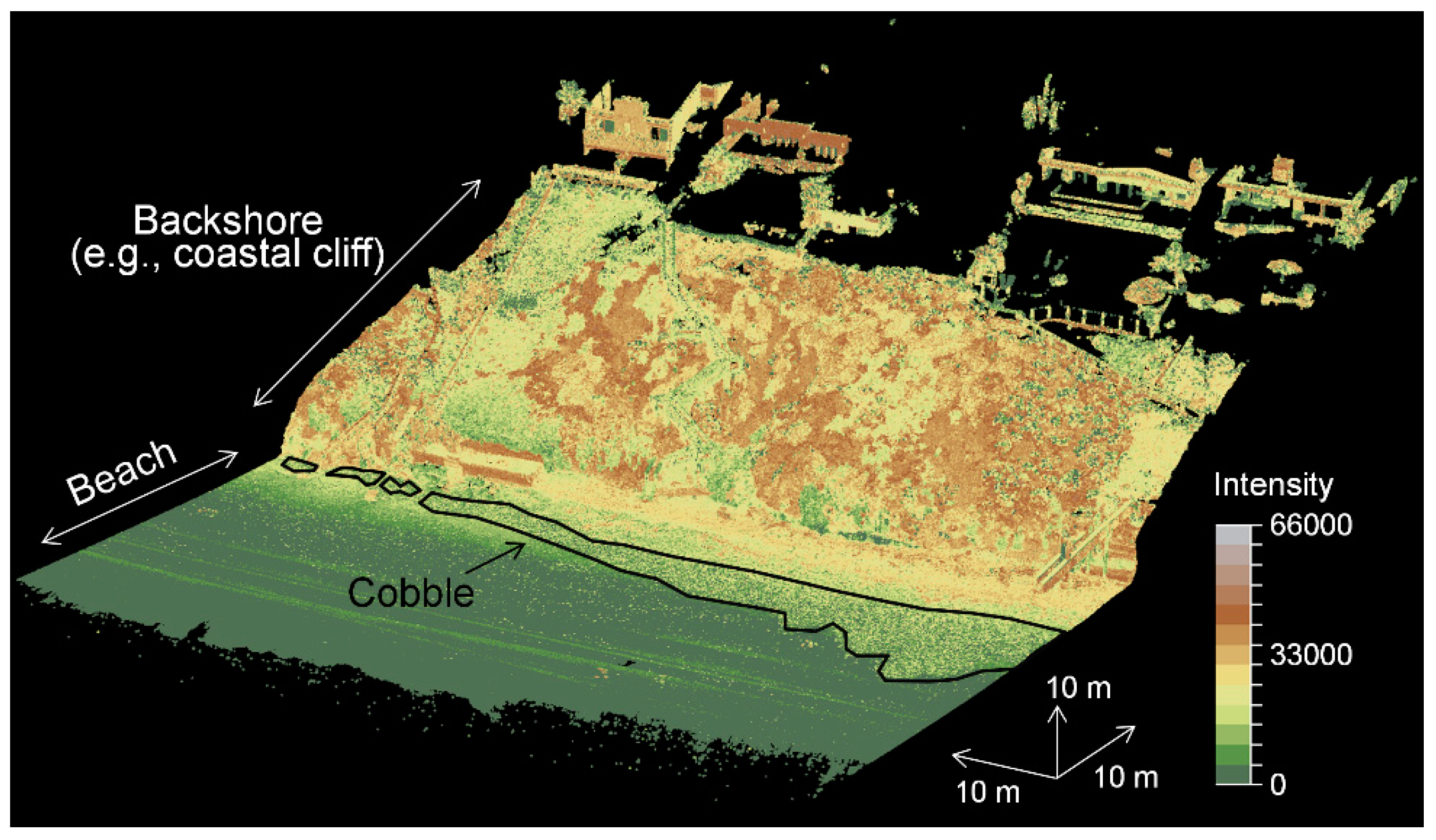
3.1. Study Area

The study area (Figure 1a, ~40 km alongshore) in northern San Diego County, California, consists of mixed sand-cobble beaches backed by lowlands, lagoons, coastal cliffs, and infrastructure. Sand thickness is typically a few meters, but is occasionally reduced to zero when winter storm waves expose the underlying bedrock. The primary composition of beach sand and bedrock are quartz and sedimentary rocks (e.g., mudstone, shale, sandstone, and siltstone) [45,46,47], respectively, whereas cobbles in the study area are igneous [48]. Median sand size ranges between 0.15 and 0.28 mm (fine-medium), and mean beach slope ranges 0.01–0.08 degrees [12]. Cobbles are generally more exposed on the beach surface during winter months [8]. Cobble distributions vary from scattered surface cobbles to extensive berms (Figure 1b,c) (see also [2,7,8]). Large storm waves can mobilize cobbles and project them at structures, causing property damage [7]. Other coastal management issues include the closure of beach access pathways from migrating cobble berms [49]. Quantitative cobble observations in the region are limited, but are necessary to improve local shoreline change models (i.e., [11]).

3.2. LiDAR Data Collection and Processing

This study used a truck-mounted mobile LiDAR system equipped with a RIEGL VZ-2000 laser scanner, coupled with a geodetic grade dual-frequency Trimble BD982 global navigation satellite system and a Trimble AP20 inertial measurement unit. Table 2 summarizes the scanning settings used in this study. Data were collected while driving alongshore at about 8 km per hour (kph) during low tide. Surveys consisted of one inland looking pass, one seaward looking pass, and up to two additional passes in areas with more complex topography, for a total of 2–4 passes and overall average beach survey rate of 2–4 kph. Data processing employed a direct georeferencing solution and 100 m range cutoff filter. The resulting point clouds contained beaches, ocean waves, and backshore features such as coastal cliffs (Figure 2). The typical beach point density was about 1000–3000 points per square meter with accuracies of a few centimeters (e.g., [50]). Point clouds were filtered and edited to remove erroneous points such as flying birds and humans on beaches [51].

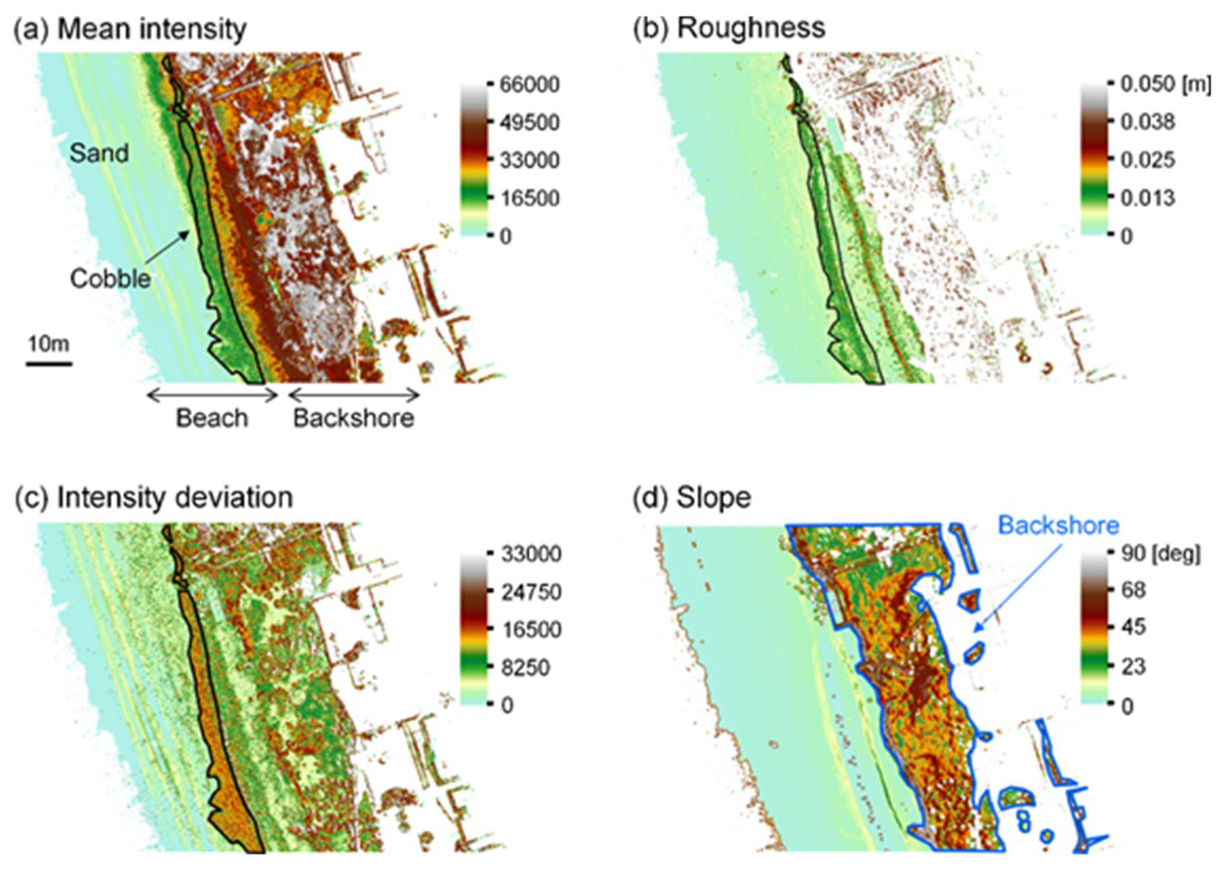
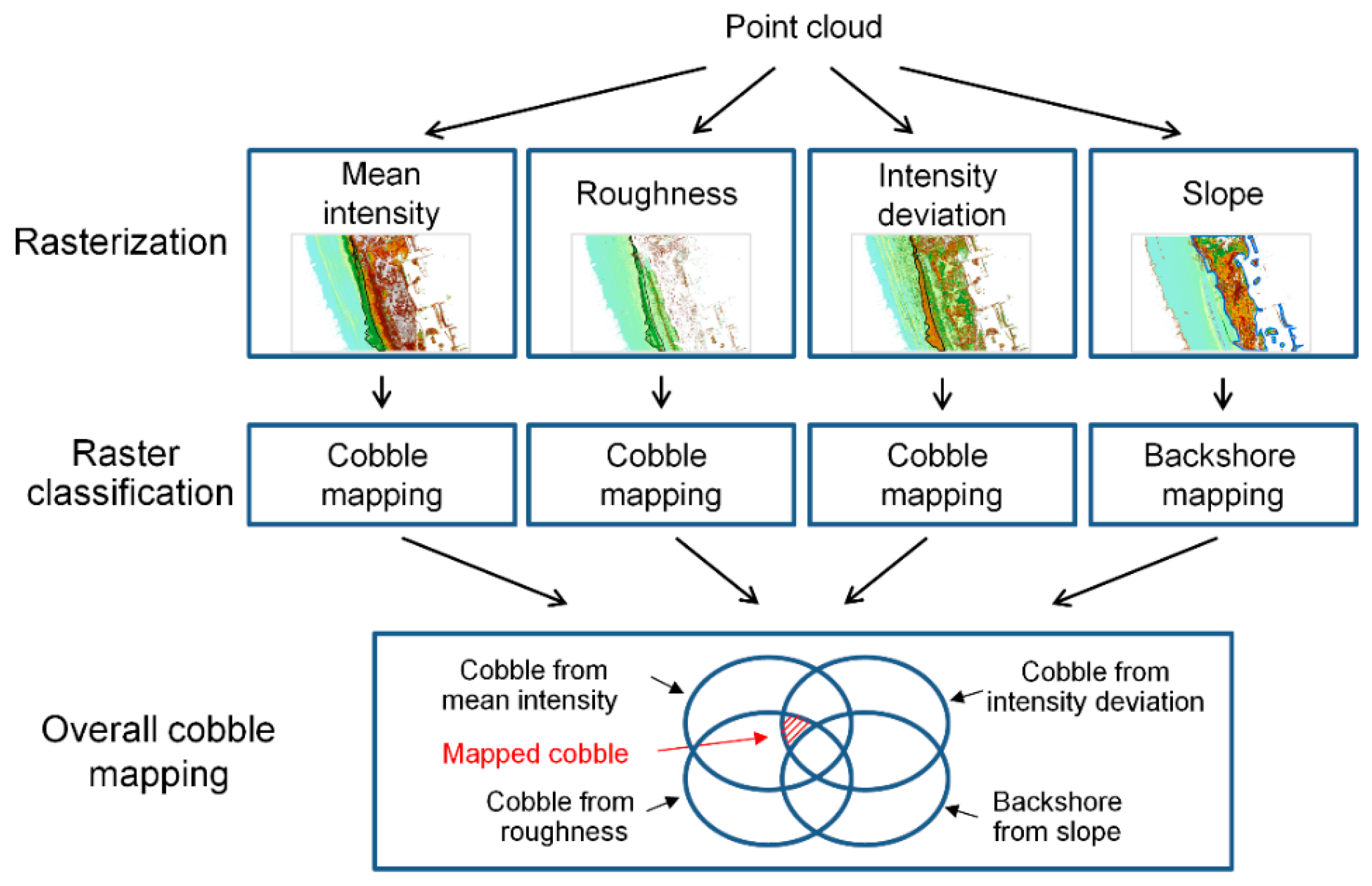
3.3. Raster Based Cobble Detection

To automatically map cobbles, this study used a raster-based classification approach. Similar to previous studies [37,38], this study used mean LiDAR intensity (Figure 3a, normalized and corrected for laser signal decay with distance, i.e., reflectance value) and topographic roughness rasters (Figure 3b), and additionally utilized intensity deviation and slope rasters (Figure 3c,d). The intensity deviation raster was used to exclude non-cobble areas having similar mean intensity and roughness values to cobble areas. The slope raster was used to exclude non-cobble backshore regions with high slopes.
Intensity deviation and roughness rasters were generated using Equation (1), where v i , v ¯ , and N are the individual point values (intensity, or elevation for roughness), mean value of points, and the number of points within a pixel, respectively. The slope raster was calculated as an average slope considering mean elevations of the eight surrounding raster pixels.
S Q R T ( ( i = 1 N ( v i v ¯ ) 2 ) / N )
The potential cobble areas were determined as raster pixels classified as “cobble” in the mean intensity, roughness, and intensity deviation rasters, and “non-backshore” in the slope raster (Figure 4). Quick Terrain Modeler (Applied Imagery, Silver Spring, MD, USA) was used to generate rasters (Universal Transverse Mercator Zone 11N coordinate system) at five different pixel sizes (5, 7.5, 10, 20, and 50 cm) to determine optimum raster resolution for automated cobble mapping (e.g., Reference [52]). The multi-raster combination approach presented here improves cobble mapping accuracy because several raster metrics are used, helping to eliminate areas mapped as cobble by one metric, but non-cobble by a different metric.

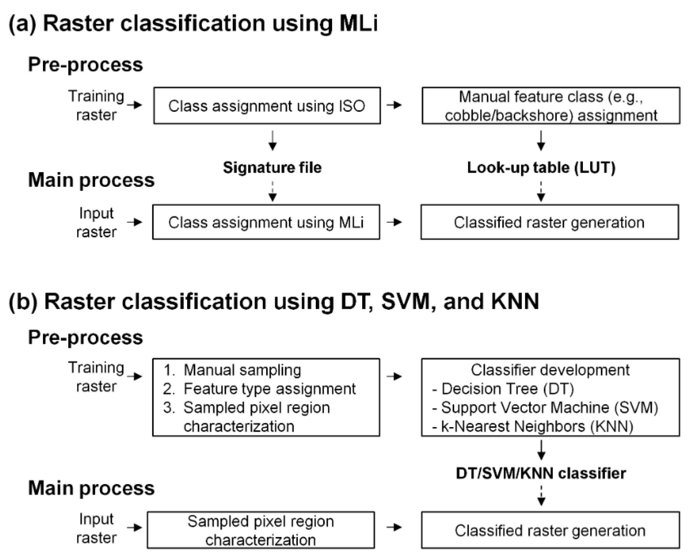
3.4. Raster Classification

This study examined four algorithms for automated machine learning-based supervised raster classification including maximum likelihood (MLi), decision tree (DT), support vector machine (SVM), and k-nearest neighbors (KNN) (Figure 5). Each algorithm used four training rasters of mean intensity, roughness, intensity deviation, and the slope generated from a ~70 m alongshore section (shown in Figure 2) with known cobble and backshore locations.
To implement MLi supervised classification, a signature file and a look up table (LUT) were established from the training rasters (Figure 5a, pre-process). First, unsupervised classification using an iterative self-organizing clustering algorithm (ISO, [53]) was applied to the training rasters to generate pixel classes and the associated signature files. Next, each feature class was manually designated cobble, backshore, or neither in a LUT. In the main process, input rasters were classified into pixel classes using the MLi algorithm with equal priors and the signature files (i.e., supervised classification), and were designated as cobble, backshore, or neither with the LUT. ArcGIS (Esri, Redlands, CA, USA) was used for both unsupervised and supervised raster classification with default parameters and a maximum class number of 10.
Similar to the MLi-based approach, DT, SVM, and KNN classifiers were initially established using the training rasters (Figure 5b, pre-process). First, a total of 1000 pixels were manually sampled and assigned a feature type (cobble/non-cobble or backshore/non-backshore). Five variables (minimum, maximum, mean, standard deviation, and range) characterizing the sampled pixel region (a 5 × 5 pixel block, centered on the sampled pixel) were calculated. Next, the variables and corresponding feature types were analyzed with DT, SVM, and KNN algorithms using a five-fold cross-validation technique to derive the associated DT, SVM, and KNN classifiers. In the main process, input rasters were classified using the DT, SVM, and KNN classifiers and calculated pixel block variables of the input raster. Matlab (Mathworks, Natick, MA, USA) was used for DT, SVM, and KNN classifier development with parameters and associated settings listed in Table 3.
In total, 20 combinations of pixel sizes (5, 7.5, 10, 20, and 50 cm) and raster classification techniques (MLi, DT, SDM, and KNN) were tested. The testing combinations are termed as “raster classification technique-pixel size” (e.g., MLi-5, DT-7.5, etc.) in this study.

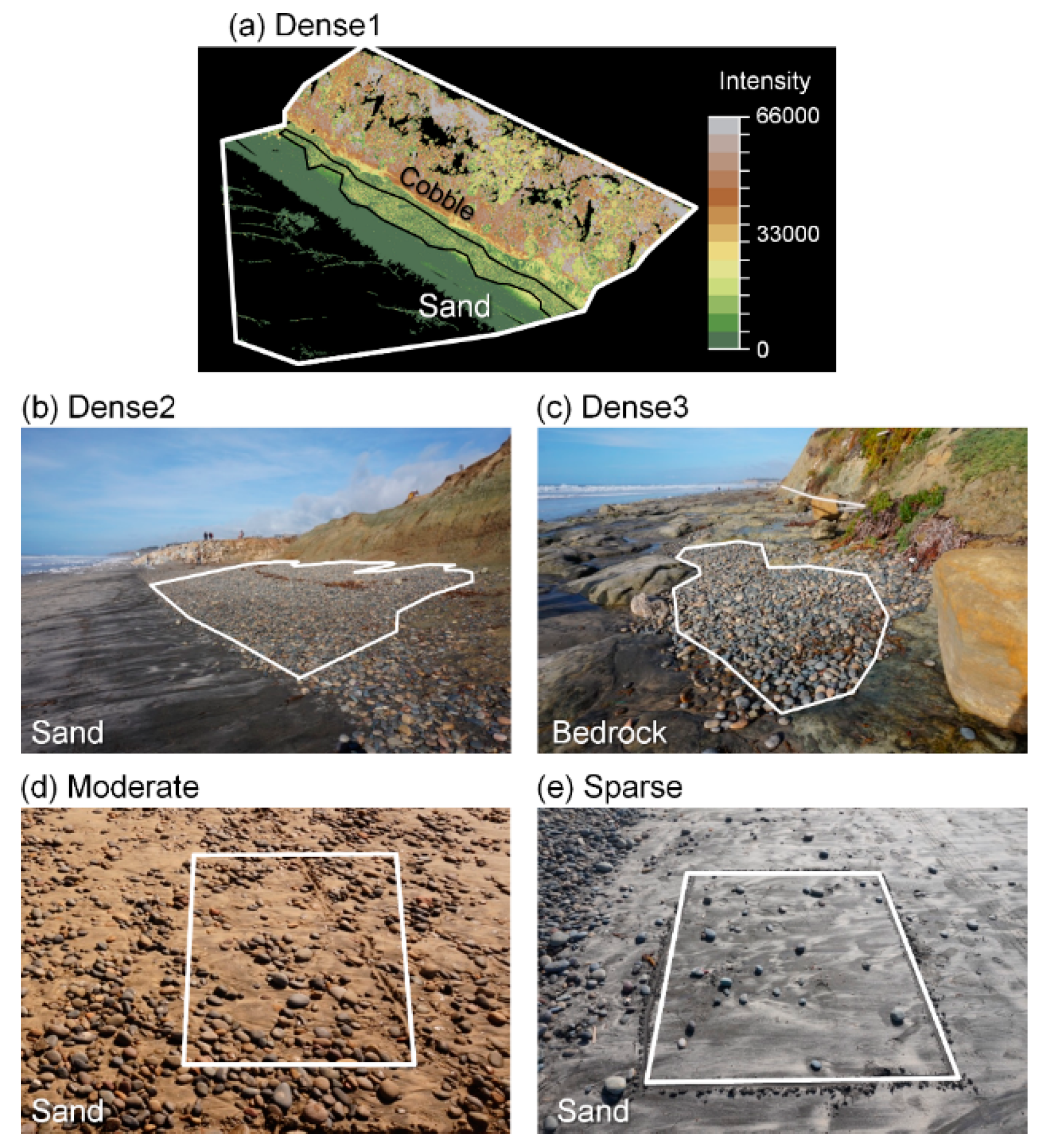
3.5. Control Site Manual Mapping

The automated cobble mapping methods were tested at five control sites with variable cobble exposure densities (three dense, one moderate, and one sparse) and beach settings (cobbles on sands and cobbles on bedrock, Figure 6). Dense1 and Dense2 sites contained cobble berms with average berm faces of 12–17 degrees, whereas Dense3 site was a cobble patch on exposed bedrock. Moderate and Sparse sites contained cobbles on low slope beaches (<5 degrees). At each control site, cobble distributions were manually mapped in the field with a Global Positioning System (GPS SPECTRA ProMark 700, Figure 6b,c), or by visually digitizing point clouds (Figure 6a) or georeferenced rectified field photographs (Figure 6d,e).
The automated mapping skill for estimating cobble coverage within a defined beach area was examined with Equation (2), where A denotes an area. Youden’s index (Equation (3)) was used to examine spatial mapping accuracy (precise location of mapped cobbles) of the automated methods relative to manual mapping. Higher Youden’s index values indicate better mapping. In Equation (3), TP (true positive) and FN (false negative) are the number of pixels manually mapped as cobble but automatically mapped as cobble and non-cobble, respectively. TN (true negative) and FP (false positive) are the number of pixels manually mapped as non-cobble but automatically mapped as non-cobble and cobble, respectively. Equation (3) was only applied to Dense1, Moderate and Sparse sites because there were no non-cobble areas manually mapped in the Dense2 and Dense3 sites.
C o b b l e   c o v e r a g e   e r r o r = A a u t o . A m a n u a l A c o n t r o l × 100   [ % ]
Y o u d e n s   i n d e x = T P T P + F N + T N T N + F P 1

4. Results

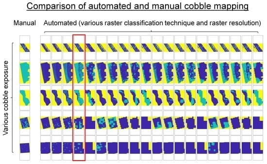
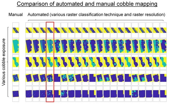
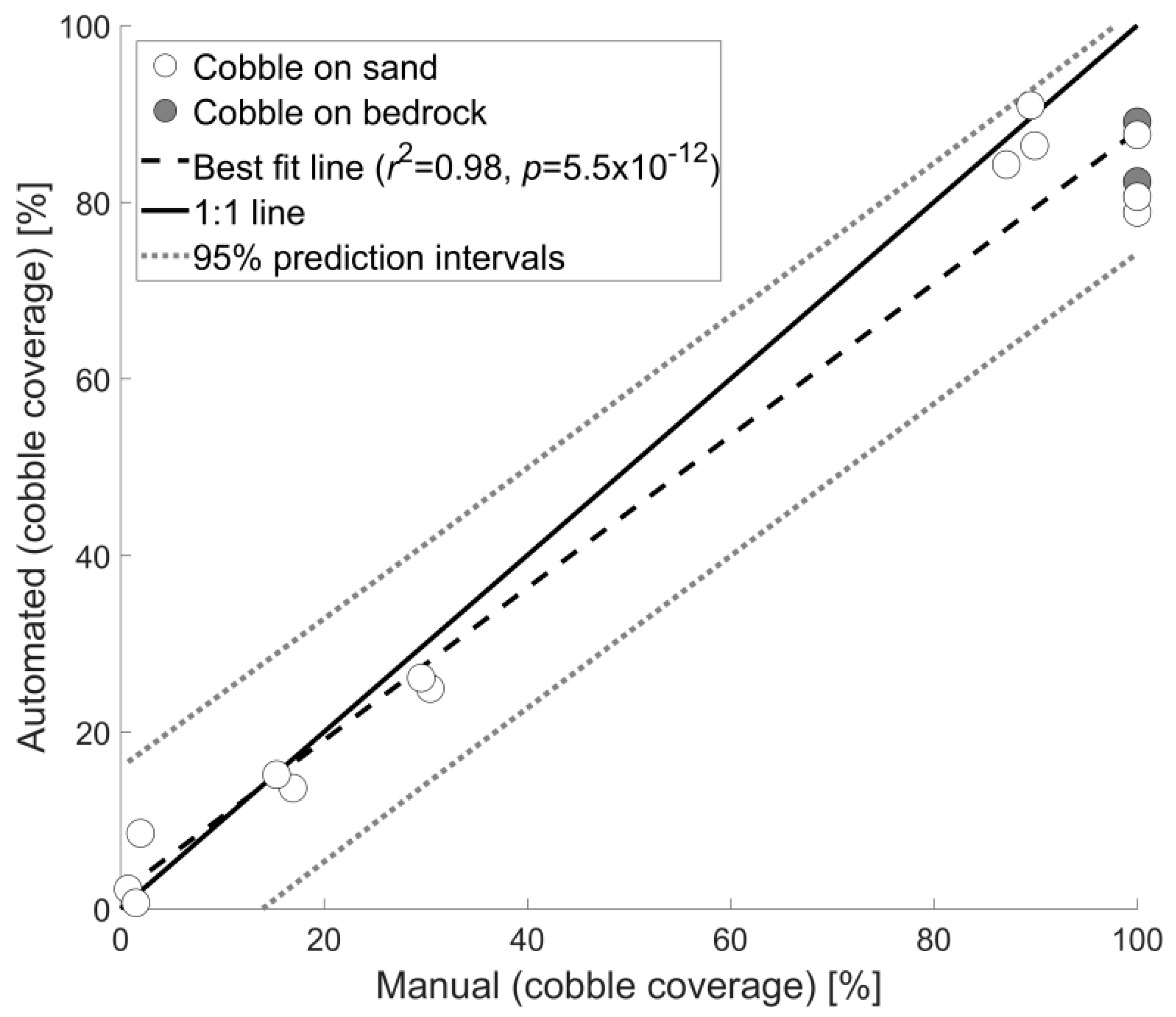
4.1. Comparison of Automated and Manual Mapping

The automated mapping capability varied depending on raster pixel size, classification technique, cobble density, and beach setting (Figure 7). For MLi methods, MLi-20 performed best, with cobble coverage errors ranging from −20 to +10%. MLi methods with smaller pixel sizes (<20 cm) largely underestimated cobbles at Dense2 and Dense3 with errors between −100 and −65%. MLi-50 produced lower errors at Dense3 (−45%) but detected zero cobble at Moderate and Sparse control sites.
DT, SVM, and KNN methods generally exhibited poor mapping capability compared to MLi. For pixel sizes 7.5 and 10 cm, all three methods produced relatively large mapping errors (−100 to −45%) at Dense2 and Dense3. For 5 cm pixel size, DT and KNN methods overestimated (>10%) cobble coverage at Moderate and Sparse control sites. Although errors at Dense1 were comparable to MLi-20, DT, SVM, and KNN methods using 10–50 cm pixel sizes detected zero cobble at the Moderate and Sparse control sites.
Youden’s index showed DT, SVM, and KNN methods generally performed better at Dense1 compared to MLi methods except for MLi-20, with Youden’s indices generally >0.5 as opposed to <0.5 for MLi methods. In contrast, Youden’s indices for Moderate and Sparse sites were relatively small (<0.25) for all methods indicating relatively poor spatial mapping for sparse-moderate cobble densities compared to Dense1.
Compared to all methods tested, MLi-20 performed best and was further tested at 10 additional control sites with a range of cobble densities and beach settings, for a total of 15 control sites. Comparison of MLi-20 automated and manual mapping of cobble coverage showed good correspondence (r2 = 0.98 and p = 5.5 × 10⁻¹², Figure 8). The best fit line indicates that, on average, MLi-20 tends to underestimate dense cobble areas, but overall errors considering all cobble densities are relatively small at <12% (best fit line) and <26% (95% prediction intervals, Figure 8).

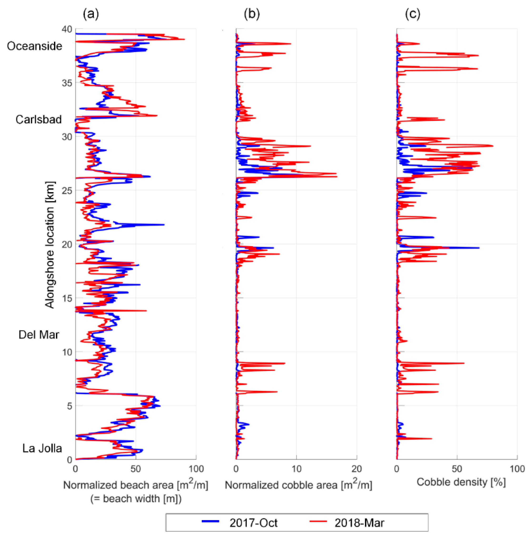
4.2. Regional Application

To test regional application, MLi-20 was applied to a ~40 km section of coast between La Jolla and Oceanside, CA (Figure 1a). LiDAR surveys were conducted over 4 consecutive days in both October 2017 (2nd–5th) and March 2018 (26th–29th) and one additional day in April 2018 (13th) to resurvey a small portion with poor data quality in the March dataset. A predefined back beach line was used to determine beach width. Beach area, cobble area (within the beach area) and surface cobble density (estimated as the cobble area divided by the beach area) were quantified at 50 m alongshore intervals between the mean high water contour (MHW, elevation 1.402 m, North American Vertical Datum 1988) and the back of the beach (Figure 9). Surface cobble coverage ranged from 0–68% in October 2017 and 0–80% in March 2018, with a mean regional increase of 2.2 ± 0.3 to 7.9 ± 1.0% (Table 4). The seasonal winter increase in cobble exposure is consistent with previous observations [8]. The largest cobble density increase, from near zero to 80%, occurred between locations 35 and 40 km in Oceanside. South Carlsbad contained notable cobble exposures (Figure 9c) consistent with previously documented locations of extensive cobble beaches [7]. Few cobbles were detected between locations 9 and 18 km (Del Mar, Figure 9) in either time period.

5. Discussion

This study demonstrates automated cobble mapping using mobile terrestrial LiDAR with relatively low errors in cobble coverage estimations (Figure 7 and Figure 8). The method is applicable to a variety of cobble and beach settings ranging from dense cobble formations (e.g., natural and artificially constructed berms [19], and dense cobbles on bedrock) to scattered beach face cobbles (e.g., Figure 1c), at both local and regional scales (Figure 9). The observed temporal (seasonal) and spatial (alongshore) cobble coverage variations quantified at regional scales can provide data needed for a better understanding of mixed sand-cobble beach system dynamics.
The presented method uses two types of rasters created from deviation operations: intensity deviation and height deviation (i.e., roughness) (Figure 3b,c). These two rasters were selected because they help differentiate cobble areas from other areas such as sand and bedrock that tend to have lower deviations. Pixel size influences both intensity and height deviations, and the results suggest that a 20 cm pixel best captures the deviation differences between cobble and other areas. These differences are not captured well for sparse and moderate areas, possibly because the deviation (roughness) contrast is lower. Despite the relatively low spatially mapping capability of precise cobble locations for sparse and moderate cobble areas, the cobble coverage errors from the method are still low (Figure 8).
The method offers several advantages over existing beach sediment mapping approaches (e.g., Table 1). The truck-mounted ground-based mobile LiDAR system allows detailed and frequent surveys of relatively large areas and permits night time data collection. Night time surveys are often useful for coastal survey applications because low tides can occur during night. Airborne-based LiDAR surveys can cover wider areas and operate at night, but are less suited to frequent and detailed surveys compared to ground-based approaches. UAV-based photogrammetry methods are capable of generating dense point clouds similar to ground based LiDAR, reduce potential shadowing because of the aerial perspective, and have been successfully applied to sediment mapping in riverine environments [40,54], but are limited to daytime lighting conditions.
The disadvantages of using a truck-mounted survey system include limitations imposed by beach access and drivable terrain. Highly rugged bedrock or steep beaches are difficult to drive and could be supplemented by airborne-based survey methods such as UAVs. The non-water penetrating LiDAR system used here limits survey coverage to subaerial topography. LiDAR is also limited to surface mapping, as opposed to sediment tracer techniques (e.g., radio frequency identification technology) which can detect subsurface cobbles down to a few tens of cm deep (e.g., [23]). Method improvement could include shallow water bathymetric surveys and subsurface cobble detection. Additional testing at other cobble and beach settings such as very steep cobble berms or moderate and sparse cobbles on bedrock are needed. The methods described here are applicable to other sites with similar beach settings and sediment distributions to the study area, but need testing before application at different sites.
Many studies (e.g., [4,11,55,56]) indicate that variation in geologic conditions including cobbles and bedrock influence morphological beach evolution. Fine sand content relative to coarse beach sediments exerts strong control on hydraulic conductivity [57], and influences beach morphology and sediment transport [58]. Bedrock location and elevation data are needed to improve beach studies which often assume homogeneous sediments with no bottom boundary [2]. The present methods allow quantitative mapping of these additional beach features (e.g., [37]) and further exploration of temporal and spatial dynamic interactions in non-homogeneous beach settings.

6. Conclusions

Cobbles influence beach morphology and can provide shoreline stability. Quantitative cobble observations at beaches are vital toward a better understanding of sand-cobble beach systems, but techniques for detailed, frequent, and large spatial scale sand-cobble beach studies are lacking. This study tested maximum likelihood, decision tree, support vector machine, and k-nearest neighbors algorithms to develop an automated raster-based cobble mapping method using mobile terrestrial LiDAR. The best performer was a method using maximum likelihood applied to 20 cm resolution rasters. The method was examined at both local (several to a few hundred square meters) and regional (~40 km of coastline) scales, and applied to a range of cobble densities and beach settings. Compared to manual mapping at control sites, cobble coverage estimation errors of the automated method were <12% (best fit) and <26% (95% prediction intervals). The method mapped the precise spatial location of dense cobble regions more accurately compared to sparse and moderate density cobble areas. The regional southern California application revealed temporal and spatial cobble distributions consistent with previous observations. The quantitative high resolution mapping methods presented here can help improve studies of mixed sand-cobble beaches.

Author Contributions

Both authors conceived and designed the study. H.M. implemented the methodology and analyzed the data. Both authors discussed the basic structure of the manuscript. H.M. wrote the initial draft, and A.P.Y. reviewed and edited. Both authors read and approved the final manuscript.

Funding

H.M. and A.P.Y. were funded by the United States Army Corps of Engineers and the California Department of Parks and Recreation, Division of Boating and Waterways Oceanography Program.

Conflicts of Interest

The authors declare no conflict of interest.

References

  1. Wentworth, C.K. A scale of grade and class terms for clastic sediments. J. Geol. 1992, 30, 377–392. [Google Scholar] [CrossRef]
  2. Holland, K.T.; Elmore, P.A. A review of heterogeneous sediments in coastal environments. Earth Sci. Rev. 2008, 89, 116–134. [Google Scholar] [CrossRef]
  3. Carter, R.W.G.; Orford, J.D. The Morphodynamics of Coarse Clastic Beaches and Barriers: A Short-and Long-term Perspective. J. Coast. Res. 1993, 15, 158–179. [Google Scholar]
  4. Jackson, D.W.T.; Cooper, J.A.G.; del Rio, L. Geological control of beach morphodynamic state. Mar. Geol. 2005, 216, 297–314. [Google Scholar] [CrossRef]
  5. Bascom, W.C. The relationship between sand size and beach-face slope. Trans. Am. Geophys. Union 1951, 32, 866–874. [Google Scholar] [CrossRef]
  6. Jennings, R.; Shulmeister, J. A field based classification scheme for gravel beaches. Mar. Geol. 2002, 186, 211–228. [Google Scholar] [CrossRef]
  7. Kuhn, G.G.; Shepard, F.P. Sea Cliffs, Beaches, and Coastal Valleys of San Diego County: Some Amazing Histories and Some Horrifying Implications; University of California Press: Berkeley, CA, USA, 1984. [Google Scholar]
  8. Everts, C.H.; Eldon, C.D.; Moore, J. Performace of Cobble Berms in Southern California. Shore Beach 2002, 70, 5–14. [Google Scholar]
  9. Schupp, R.D. A Study of the Cobble Beach Cusps along Santa Monica Bay, California. Master’s Thesis, University of Southern California, Los Angeles, CA, USA, August 1953. [Google Scholar]
  10. Shepard, F.P. Gravel Cusps on the California Coast Related to Tides. Science 1935, 82, 251–253. [Google Scholar] [CrossRef] [PubMed]
  11. Yates, M.L.; Guza, R.T.; O’Reilly, W.C.; Seymour, R.J. Overview of seasonal sand level changes on southern California beaches. Shore Beach 2009, 77, 39–46. [Google Scholar]
  12. Doria, A.; Guza, R.T.; O’Reilly, W.C.; Yates, M.L. Observations and modeling of San Diego beaches during El Niño. Cont. Shelf Res. 2016, 124, 153–164. [Google Scholar] [CrossRef] [Green Version]
  13. Carter, R.W.G.; Orford, J.D. Corse classitic barrier beaches: A discussion of the distinctive dynamic and morpho sedimentary characteristics. Mar. Geol. 1984, 60, 377–389. [Google Scholar] [CrossRef]
  14. Forbes, D.L.; Orford, J.D.; Carter, R.W.G.; Shaw, J.; Jennings, S.C. Morphodynamic evolution, self-organisation, and instability of coarse-clastic barriers on paraglacial coasts. Mar. Geol. 1995, 126, 63–85. [Google Scholar] [CrossRef]
  15. Orford, J.D.; Forbes, D.L.; Jennings, S.C. Organisational controls, typologies and time scales of paraglacial gravel-dominated coastal systems. Geomorphology 2002, 48, 51–85. [Google Scholar] [CrossRef]
  16. Bradbury, A.P.; Powell, K.A. The Short Term Profile Response of Shingle Spits to Storm Wave Action. In Proceedings of the 23rd Conference on Coastal Engineering, Venice, Italy, 4–9 October 1992. [Google Scholar]
  17. Allan, J.C.; Komar, P.D. Environmentally Compatible Cobble Berm and Artificial Dune for Shore Protection. Shore Beach 2004, 72, 9–18. [Google Scholar]
  18. Kochnower, D.; Reddy, S.M.W.; Flick, R.E. Factors influencing local decisions to use habitats to protect coastal communities from hazards. Ocean Coast. Manag. 2015, 116, 277–290. [Google Scholar] [CrossRef]
  19. Allan, J.C.; Hart, R. Profile dynamics and particle tracer mobility of a cobble berm constructed on the oregon coast. In Proceedings of the 6th International Symposium on Coastal Engineering and Science of Coastal Sediment Processes, New Orleans, LA, USA, 13–17 May 2007. [Google Scholar]
  20. Forbes, D.L.; Taylor, R.B.; Orford, J.D.; Carter, R.W.G.; Shaw, J. Gravel-barrier migration and overstepping. Mar. Geol. 1991, 97, 305–313. [Google Scholar] [CrossRef]
  21. Allan, J.C.; Hart, R.; Tranquili, J.V. The use of Passive Integrated Transponder (PIT) tags to trace cobble transport in a mixed sand-and-gravel beach on the high-energy Oregon coast, USA. Mar. Geol. 2006, 232, 63–86. [Google Scholar] [CrossRef]
  22. Curtiss, G.M.; Osborne, P.D.; Horner-Devine, A.R. Seasonal patterns of coarse sediment transport on a mixed sand and gravel beach due to vessel wakes, wind waves, and tidal currents. Mar. Geol. 2009, 259, 73–85. [Google Scholar] [CrossRef]
  23. Dickson, M.E.; Kench, P.S.; Kantor, M.S. Longshore transport of cobbles on a mixed sand and gravel beach, southern Hawke Bay, New Zealand. Mar. Geol. 2011, 287, 31–42. [Google Scholar] [CrossRef]
  24. Stark, N.; Hay, A.E. Pebble and cobble transport on a steep, mega-tidal, mixed sand and gravel beach. Mar. Geol. 2016, 382, 210–223. [Google Scholar] [CrossRef]
  25. Kench, P.S.; Beetham, E.; Bosserelle, C.; Kruger, J.; Pohler, S.M.L.; Coco, G.; Ryan, E.J. Nearshore hydrodynamics, beachface cobble transport and morphodynamics on a Pacific atoll motu. Mar. Geol. 2017, 389, 17–31. [Google Scholar] [CrossRef]
  26. Adams, P.N.; Ruggiero, P.; Schoch, G.C.; Gelfenbaum, G. Intertidal sand body migration along a megatidal coast, Kachemak Bay, Alaska. J. Geophys. Res. Earth Surf. 2007, 112, F02007. [Google Scholar] [CrossRef]
  27. Ruggiero, P.; Adams, P.N.; Warrick, J.A. Mixed Sediment Beach Processes: Kachemak Bay, ALASKA. In Proceedings of the 6th International Symposium on Coastal Engineering and Science of Coastal Sediment Processes, New Orleans, LA, USA, 13–17 May 2007. [Google Scholar]
  28. Pérez-Alberti, A.; Trenhaile, A.S. An initial evaluation of drone-based monitoring of boulder beaches in Galicia, north-western Spain. Earth Surf. Process. Landforms 2015, 40, 105–111. [Google Scholar] [CrossRef]
  29. Rubin, D.M. A Simple Autocorrelation Algorithm for Determining Grain Size from Digital Images of Sediment. J. Sediment. Res. 2004, 74, 160–165. [Google Scholar] [CrossRef]
  30. Barnard, P.L.; Rubin, D.M.; Harney, J.; Mustain, N. Field test comparison of an autocorrelation technique for determining grain size using a digital ‘beachball’ camera versus traditional methods. Sediment. Geol. 2007, 201, 180–195. [Google Scholar] [CrossRef]
  31. Buscombe, D.; Masselink, G. Grain-size information from the statistical properties of digital images of sediment. Sedimentology 2009, 56, 421–438. [Google Scholar] [CrossRef]
  32. Warrick, J.A.; Rubin, D.M.; Ruggiero, P.; Harney, J.N.; Draut, A.E.; Buscombe, D. Cobble cam: Grain-size measurements of sand to boulder from digital photographs and autocorrelation analyses. Earth Surf. Process. Landforms 2009, 34, 1811–1821. [Google Scholar] [CrossRef]
  33. Carbonneau, P.E.; Lane, S.N.; Bergeron, N.E. Catchment-scale mapping of surface grain size in gravel bed rivers using airborne digital imagery. Water Resour. Res. 2004, 40, W07202. [Google Scholar] [CrossRef]
  34. Carbonneau, P.E.; Bergeron, N.; Lane, S.N. Automated grain size measurements from airborne remote sensing for long profile measurements of fluvial grain sizes. Water Resour. Res. 2005, 41, W11426. [Google Scholar] [CrossRef]
  35. Deronde, B.; Houthuys, R.; Debruyn, W.; Fransaer, D.; Van Lancker, V.; Henriet, J.-P. Use of Airborne Hyperspectral Data and Laserscan Data to Study Beach Morphodynamics along the Belgian Coast. J. Coast. Res. 2006, 22, 1108–1117. [Google Scholar] [CrossRef]
  36. Deronde, B.; Houthuys, R.; Henriet, J.-P.; Van Lancker, V. Monitoring of the sediment dynamics along a sandy shoreline by means of airborne hyperspectral remote sensing and LiDAR: A case study in Belgium. Earth Surf. Process. Landforms 2008, 33, 280–294. [Google Scholar] [CrossRef]
  37. Beasy, C.; Hopkinson, C.; Webster, T. Classification of nearshore materials on the Bay of Fundy coast using LiDAR intensity data. In Proceedings of the 26th Canadian Symposium on Remote Sensing, Walfville, NS, Canada, 14–16 June 2005. [Google Scholar]
  38. Cottin, A.G.; Forbes, D.L.; Long, B.F. Shallow seabed mapping and classification using waveform analysis and bathymetry from SHOALS lidar data. Can. J. Remote Sens. 2009, 35, 422–434. [Google Scholar] [CrossRef]
  39. Fairley, R.D.; Thomas, I.; Phillips, T.; Reeve, D. Terrestrial Laser Scanner Techniques for Enhancement in Understanding of Coastal Environments. In Seafloor Mapping along Continental Shelves: Research and Techniques for Visualizing Benthic Environments (Coastal Research Library); Finkl, C.W., Makowski, C., Eds.; Springer International Publishing: Zürich, Switzerland, 2016; pp. 273–289. ISBN 978-3-319-25121-9. [Google Scholar]
  40. Woodget, A.S.; Austrums, R. Subaerial grain size measurement using topographic data derived from a UAV-SfM approach. Earth Surf. Process. Landforms 2017, 42, 1434–1443. [Google Scholar] [CrossRef]
  41. Brock, J.C.; Purkis, S.J. The Emerging Role of Lidar Remote Sensing in Coastal Research and Resource Management. J. Coast. Res. 2009, 25, 1–5. [Google Scholar] [CrossRef]
  42. Young, A.P. Decadal-scale coastal cliff retreat in southern and central California. Geomorphology 2018, 300, 164–175. [Google Scholar] [CrossRef]
  43. Matsumoto, H.; Dickson, M.E.; Masselink, G. Systematic analysis of rocky shore platform morphology at large spatial scale using LiDAR-derived digital elevation models. Geomorphology 2017, 286, 45–57. [Google Scholar] [CrossRef]
  44. Webster, T.L.; Forbes, D.L.; Dickie, S.; Shreenan, R. Using topographic lidar to map flood risk from storm-surge events for Charlottetown, Prince Edward Island, Canada. Can. J. Remote Sens. 2004, 30, 64–76. [Google Scholar] [CrossRef]
  45. Inman, D.L.; Zampol, J.A.; White, T.E.; Hanes, D.M.; Waldorf, B.W.; Kastens, K.A. Feild measurements of sand motion in the surf zone. In Proceedings of the 17th International Symposium on Coastal Engineering, Sydney, Australia, 23–28 March 1980. [Google Scholar]
  46. Kennedy, M.P. Geology of the San Diego metropolitan area, western area. Geotherm. Resour. Counc. Trans. 1975, 27, 765–770. [Google Scholar]
  47. Young, A.P.; Raymond, J.H.; Sorenson, J.; Johnstone, E.A.; Driscll, N.W.; Flick, R.E.; Guza, R.T. Coarse sediment yields from seacliff erosion in the Oceanside Littoral Cell. J. Coast. Res. 2010, 26, 580–585. [Google Scholar] [CrossRef]
  48. Abbott, P. The Rise and Fall of San Diego: 150 Million Years of History Recorded in Sedimentary Rocks; Sunblet Publications, Inc.: San Diego, CA, USA, 1999; ISBN 9780932653314. [Google Scholar]
  49. Young, A.P.; Flick, R.E.; Gallien, T.W.; Giddings, S.N.; Guza, R.T.; Hayvey, M.; Lenain, L.; Ludka, B.C.; Melville, W.L.; O’Reilly, W.C. Southern California Coastal Response to the 2015-16 El Niño. J. Geophys. Res. Earth Surf. 2018. under review. [Google Scholar]
  50. Nolan, J.; Eckels, R.; Olsen, M.J.; Yen, K.S.; Lasky, T.A.; Ravani, B. Analysis of the Multipass Approach for Collection and Processing of Mobile Laser Scan Data. J. Surv. Eng. 2017, 143, 04017004. [Google Scholar] [CrossRef]
  51. Cunningham, K.; Olsen, M.J.; Wartman, J.; Dunham, L. A Platform for Proactive, Risk-Based Slope Asset Management, Phase II; Pactrans Report 2013-M-UAF-0042; Pacific Northwest Transportation Consortium: Seattle, WA, USA, 2015. [Google Scholar]
  52. Usery, E.L.; Finn, M.P.; Scheidt, D.J.; Ruhl, S.; Beard, T.; Bearden, M. Geospatial data resampling and resolution effects on watershed modeling: A case study using the agricultural non-point source pollution model. J. Geogr. Syst. 2004, 6, 289–306. [Google Scholar] [CrossRef]
  53. Ball, G.H.; Hall, D.J. ISODATA, A Novel Method of Data Analysis and Pattern Classification; Standford Research Institutie: Melon Park, CA, USA, 1965; Volume 699. [Google Scholar]
  54. Vázquez-Tarrío, D.; Borgniet, L.; Liébault, F.; Recking, A. Using UAS optical imagery and SfM photogrammetry to characterize the surface grain size of gravel bars in a braided river (Vénéon River, French Alps). Geomorphology 2017, 285, 94–105. [Google Scholar] [CrossRef]
  55. Anthony, E.J. Sediment-wave parametric characterization of beaches. J. Coast. Res. 1998, 14, 347–352. [Google Scholar]
  56. Scott, T.; Masselink, G.; Russell, P. Morphodynamic characteristics and classification of beaches in England and Wales. Mar. Geol. 2011, 286, 1–20. [Google Scholar] [CrossRef] [Green Version]
  57. Mason, T.; Coates, T.T. Sediment Transport Processes on Mixed Beaches: A Review for Shoreline Management. J. Coast. Res. 2001, 17, 645–657. [Google Scholar]
  58. Quick, M.C. Onshore-offshore sediment transport on beaches. Coast. Eng. 1991, 15, 313–332. [Google Scholar] [CrossRef]
Figure 1. (a) Southern California study area and example cobble exposures of (b) dense upper-beach cobble berm, and (c) mid-beach cobble patches.
Remotesensing 10 01253 g001
Figure 2. Example of a 3-D point cloud obtained from the mobile LiDAR system, colored by return intensity. Black lines enclose manually delineated dense cobble surface exposures.
Remotesensing 10 01253 g002
Figure 3. Rasters (20 cm resolution, location shown in Figure 2) of (a) mean intensity, (b) roughness, (c) intensity deviation, and (d) slope. Black and blue lines show manually delineated cobble and backshore areas, respectively.
Remotesensing 10 01253 g003
Figure 4. Flowchart of the automated cobble mapping method.
Remotesensing 10 01253 g004
Figure 5. Pre- and main process flowcharts of supervised raster classification using (a) maximum likelihood (MLi), and (b) decision tree (DT), support vector machine (SVM), and k-nearest neighbors (KNN).
Remotesensing 10 01253 g005
Figure 6. Manually mapped control sites used to test automated cobble mapping. (a,b) Dense cobble exposure on sand, (c) dense cobble exposure on bedrock, (d) moderate cobble exposure on sand, and (e) sparse cobble exposure on sand. Areas enclosed by white lines indicate the areas examined, and a black line in 6a encloses dense cobble surface exposures. Points in 6a are colored by intensity.
Remotesensing 10 01253 g006
Figure 7. (a) Comparison of manual and automated cobble mapping methods at the control sites, and the associated (b) cobble coverage mapping errors and (c) Youden’s index. Green, blue, and yellow pixels in 7a indicate areas of cobble, non-cobble and no data, respectively. The red box highlights the results of the best performer.
Remotesensing 10 01253 g007
Figure 8. Comparison of MLi-20 automated and manual cobble mapping for a range of cobble densities and beach settings.
Remotesensing 10 01253 g008
Figure 9. Regional application of automated MLi-20 cobble mapping in southern California for October 2017 and March 2018. (a) Beach area normalized by 50 m alongshore interval (beach width), (b) cobble area normalized by 50 m alongshore interval, and (c) cobble density. Beach width was measured from MHW to the back beach line.
Remotesensing 10 01253 g009
Table 1. Examples of remotely-sensed beach sedimentary mapping techniques. Sediment sizes (larger than sands) are shown where available.
Survey ToolRemotely Sensed DataData PropertyData ResolutionMapping TechniqueSediment Type (Size)References
Multiple video camerasDigital imagery--Manual mappingSands to coarse sediments (1~3 m)[26,27]
UAVDigital imagery-7.5 mmManual mappingCoarse sediments (>75 mm)[28]
Single cameraDigital imagery(Grayscaled) image intensity2.5–7.9 × 10⁻² mmAutocorrelationSands to coarse sediments (<~20 mm)[30,31]
AirborneHyperspectral imageryReturn signal spectrum2 mRaster classificationFine to coarse sands containing shells and gravels[35,36]
AirborneLiDAR point cloudLiDAR intensity, topographic roughness and luminance2 mRaster classificationCobbles (to bedrock)[37]
AirborneLiDAR point cloudLiDAR intensity, topographic roughness, kurtosis and skewness2–4 mRaster classification(Under water) fine sands, cobble/boulder (>256 mm) and bedrock [38]
Terrestrial (static)LiDAR point cloudLiDAR RGB color, topographic roughness0.1 mArtificial neural network grouping (RGB color)Sands to gravels (49 1 mm)[39]
UAVDigital imagery, and SfM point cloudImage texture, and topographic roughness1–5 cmCorrelation analysis of grain size and negative entropy/roughnessCobbles to boulders[40] 2
1D50 median grain size, 2 applied to gravel bed river.
Table 2. Scanning settings.
ItemSetting
Laser pulse frequency550,000 Hz
Ranging precision5 mm
Multi-target detectionApplied
Online waveform processingApplied
Scan modeLine scan
Scanner height from the ground2.5–2.6 m
Grazing scan angle range on beach surface1.5–40°
Table 3. Parameters and settings used in DT, SVM, and KNN classifier development.
ClassifierParameterSettings
DTMaximum number of splits4
Split criterionGini’s diversity index
SVMKernel functionGaussian
Kernel scale0.56
Box constraint level1
Multiclass methodOne-vs-One
KNNNumber of Neighbors10
Distance metricEuclidean
Table 4. Regional cobble density comparison between October 2017 and March 2018. Mean values consider the mapping error (<12%, best fit line, Figure 8).
SurveyMinimumMaximumMean
October 20170.0%68%2.2 ± 0.3%
March 20180.0%80%7.9 ± 1.0%

