Systematic Comparison of Power Line Classification Methods from ALS and MLS Point Cloud Data


Abstract
1. Introduction
2. Materials and Methods
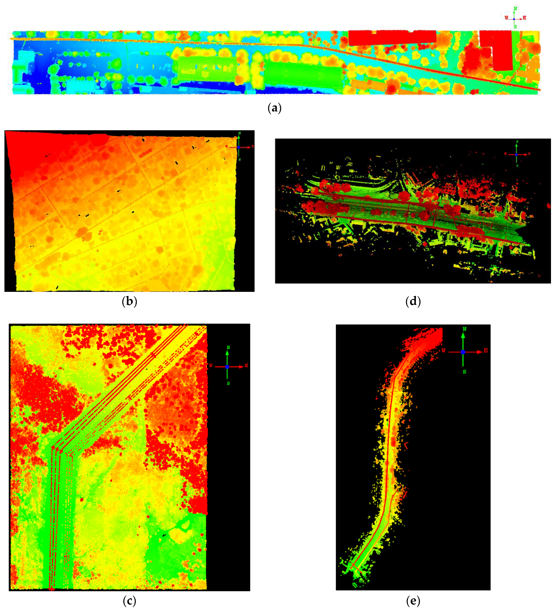
2.1. Dataset
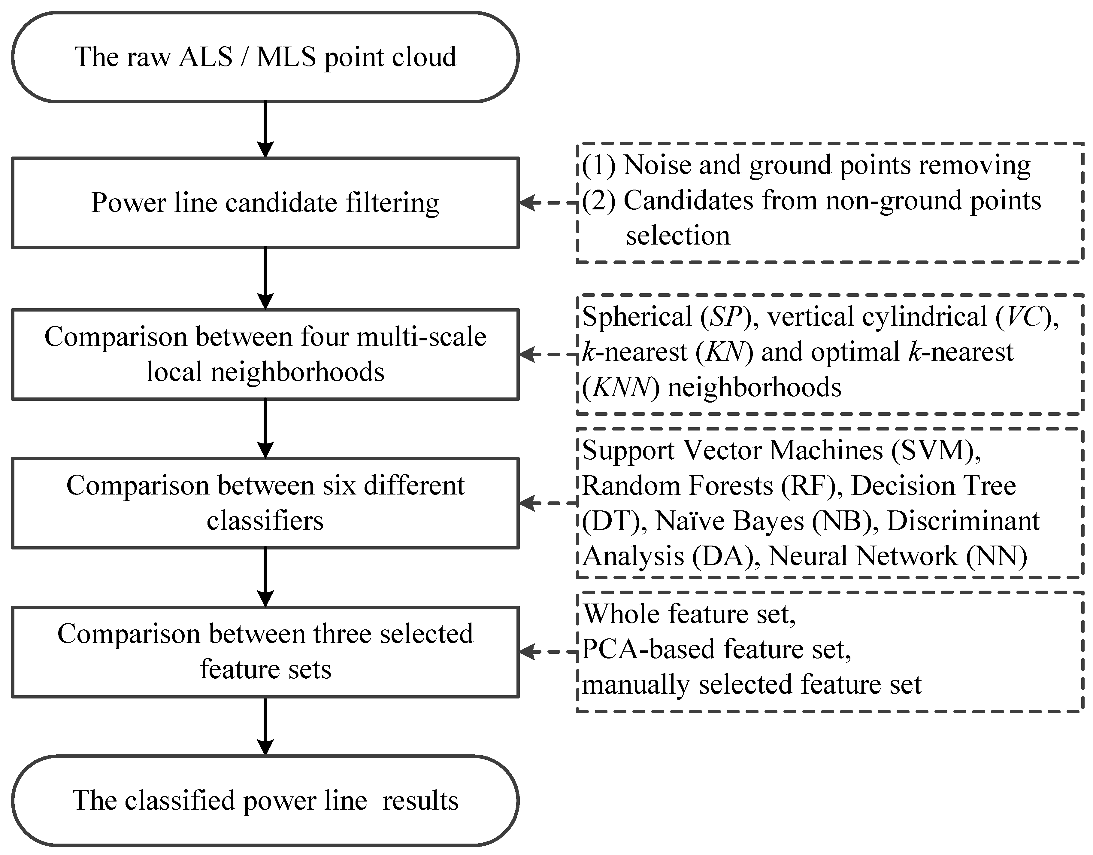
2.2. Power Line Candidate Filtering
2.3. Multi-Scale Neighborhood Based Feature Selection
2.3.1. Local Neighborhood Determination
- a spherical neighborhood is formed by all of the 3D points within a sphere around point P, which is parameterized with a fixed radius,
- a vertical cylindrical neighborhood is formed by all of the 3D points within a vertical cylindrical whose axis vertically passes through point P and whose radius is fixed,
- a k-nearest neighborhood is formed by the nearest neighbors of considered point P, the k is its parameter,
- an optimal k-nearest neighborhood is formed by the optimal k-nearest neighbors based on the above-mentioned k-nearest neighborhood, the optimal k is derived by eigenentropy-based scale selection.
2.3.2. Feature Extraction
2.4. Classifiers
2.4.1. Support Vector Machines (SVM)
2.4.2. Random Forest (RF)
2.4.3. Decision Tree (DT)
2.4.4. Naive Bayes (NB)
2.4.5. Discriminant Analysis (DA)
2.4.6. Neural Network (NN)
2.5. Experiments
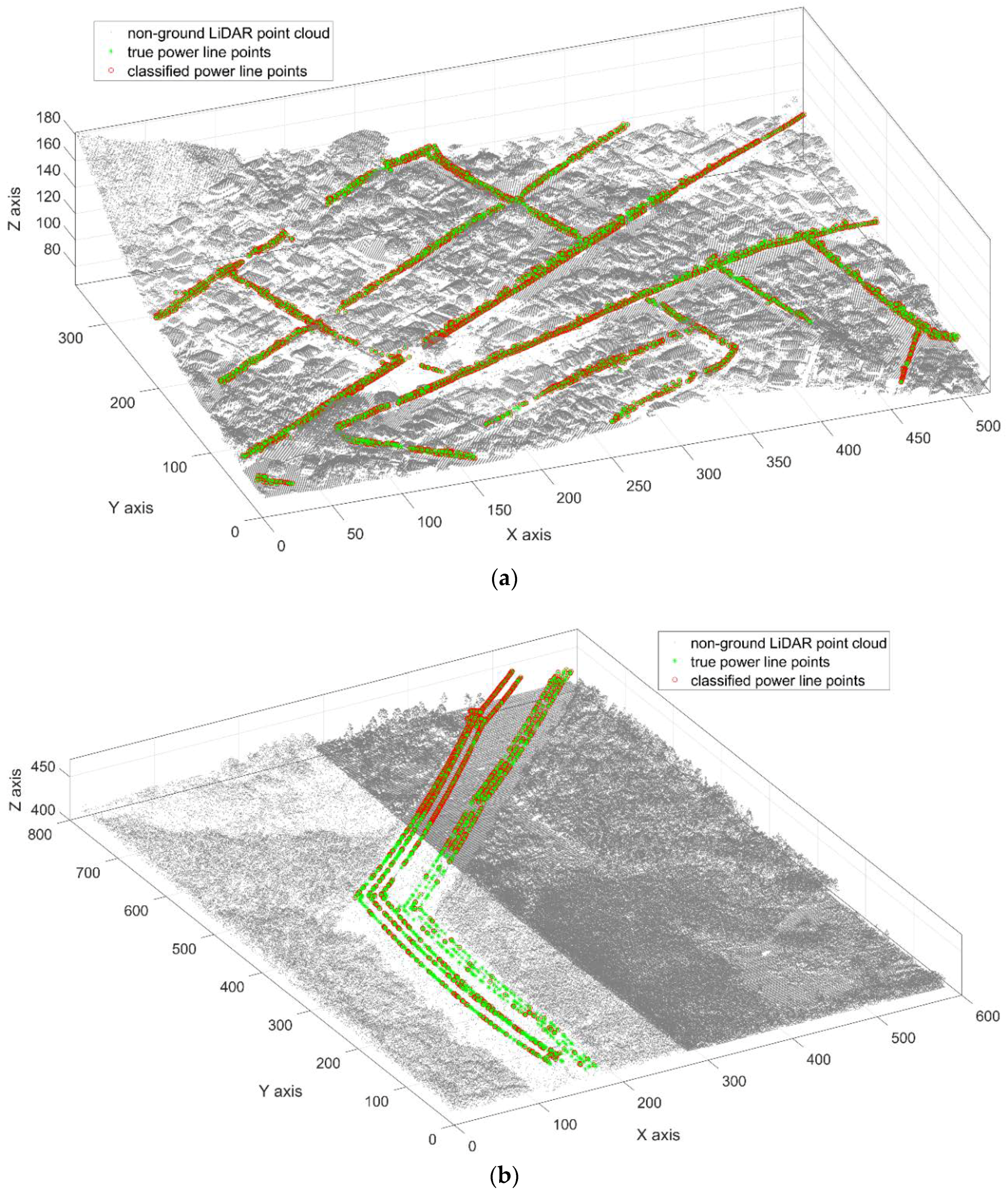
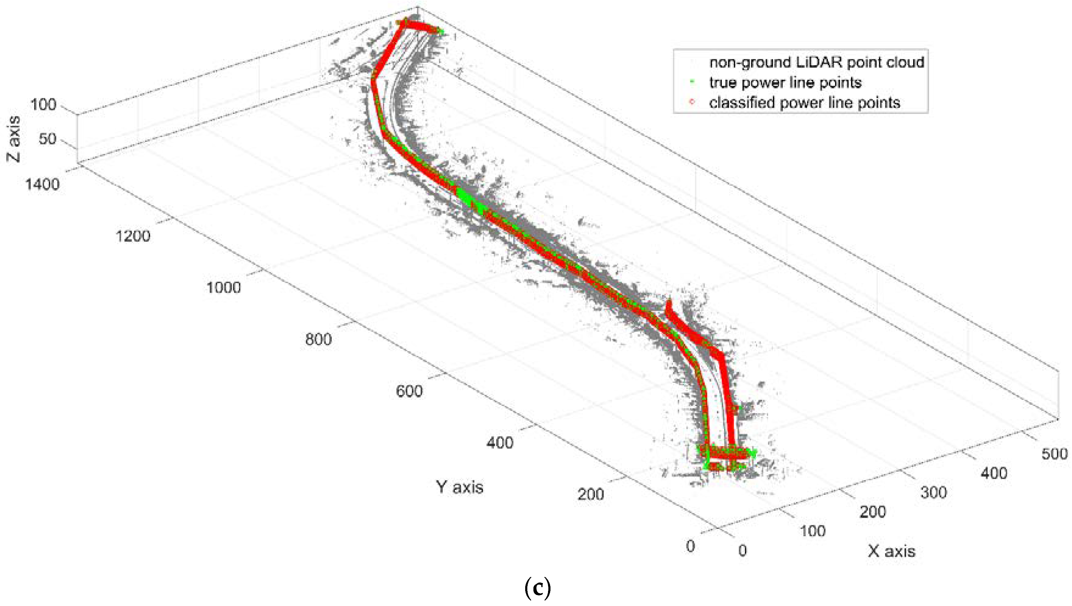
3. Results
3.1. Multiple Comparisons between Neighborhood Types
3.2. Comparisons Between Classifiers
3.3. Comparisons between Selected Feature Sets
4. Discussion
4.1. Sensitivity Analysis of Local Neighborhood
4.2. Effects of Different Classifiers
4.3. Differences between Selected Feature Sets
5. Conclusions
Author Contributions
Funding
Acknowledgments
Conflicts of Interest
References
- Ahmad, J.; Malik, A.S.; Xia, L.; Ashikin, N. Vegetation encroachment monitoring for transmission lines right-of-ways: A survey. Electr. Power Syst. Res. 2013, 95, 339–352. [Google Scholar] [CrossRef]
- Matikainen, L.; Lehtomäki, M.; Ahokas, E.; Hyyppä, J.; Karjalainen, M.; Jaakkola, A.; Kukko, A.; Heinonen, T. Remote sensing methods for power line corridor surveys. ISPRS J. Photogramm. Remote Sens. 2016, 119, 10–31. [Google Scholar] [CrossRef]
- Glennie, C.L.; Carter, W.E.; Shrestha, R.L.; Dietrich, W.E. Geodetic imaging with airborne lidar: The earth’s surface revealed. Rep. Prog. Phys. Phys. Soc. 2013, 76, 8. [Google Scholar] [CrossRef] [PubMed]
- McManamon, P.F. Review of ladar: A historic, yet emerging, sensor technology with rich phenomenology. Opt. Eng. 2012, 51, 060901. [Google Scholar] [CrossRef]
- Zhang, Y.; Yuan, X.; Fang, Y.; Chen, S. Uav low altitude photogrammetry for power line inspection. ISPRS Int. J. Geo-Inf. 2017, 6, 14. [Google Scholar] [CrossRef]
- Kwoczyńska, B.; Dobek, J. Elaboration of the 3D model and survey of the power lines using data from airborne laser scanning. J. Ecol. Eng. 2016, 17, 65–74. [Google Scholar] [CrossRef]
- Popovic, D.; Pajic, V.; Jovanovic, D.; Sabo, F.; Radovic, J. Semi-automatic classification of power lines by using airborne lidar. In FIG Working Week 2017, Surveying the World of Tomorrow—From Digitalisation to Augmented Reality; International Federation of Surveyors FIG: Helsinki, Finland, 2017. [Google Scholar]
- Cheng, L.; Tong, L.; Wang, Y.; Li, M. Extraction of urban power lines from vehicle-borne lidar data. Remote Sens. 2014, 6, 3302–3320. [Google Scholar] [CrossRef]
- Blomley, R.; Jutzi, B.; Weinmann, M. Classification of airborne laser scanning data using geometric multi-scale features and different neighbourhood types. ISPRS Ann. Photogramm. Remote Sens. Spat. Inf. Sci. 2016, III-3, 169–176. [Google Scholar] [CrossRef]
- Weinmann, M.; Jutzi, B.; Hinz, S.; Mallet, C. Semantic point cloud interpretation based on optimal neighborhoods, relevant features and efficient classifiers. ISPRS J. Photogramm. Remote Sens. 2015, 105, 286–304. [Google Scholar] [CrossRef]
- Weinmann, M.; Schmidt, A.; Mallet, C.; Hinz, S.; Rottensteiner, F.; Jutzi, B. Contextual classification of point cloud data by exploiting individual 3D neigbourhoods. ISPRS Ann. Photogramm. Remote Sens. Spat. Inf. Sci. 2015, II-3/W4, 271–278. [Google Scholar] [CrossRef]
- Weinmann, M.; Urban, S.; Hinz, S.; Jutzi, B.; Mallet, C. Distinctive 2D and 3D features for automated large-scale scene analysis in urban areas. Comput. Graph. 2015, 49, 47–57. [Google Scholar] [CrossRef]
- Yang, B.; Huang, R.; Li, J.; Tian, M.; Dai, W.; Zhong, R. Automated reconstruction of building lods from airborne lidar point clouds using an improved morphological scale space. Remote Sens. 2017, 9, 14. [Google Scholar] [CrossRef]
- Kim, H.B.; Sohn, G. Point-based classification of power line corridor scene using random forests. Photogramm. Eng. Remote Sens. 2013, 79, 821–833. [Google Scholar] [CrossRef]
- Guo, B.; Li, Q.; Huang, X.; Wang, C. An improved method for power-line reconstruction from point cloud data. Remote Sens. 2016, 8, 36. [Google Scholar] [CrossRef]
- Guo, B.; Huang, X.; Zhang, F.; Sohn, G. Classification of airborne laser scanning data using jointboost. ISPRS J. Photogramm. Remote Sens. 2015, 100, 71–83. [Google Scholar] [CrossRef]
- Jwa, Y.; Sohn, G. A piecewise catenary curve model growing for 3D power line reconstruction. Photogramm. Eng. Remote Sens. 2012, 78, 1227–1240. [Google Scholar] [CrossRef]
- Jwa, Y.; Sohn, G.; Kim, H.B. Automatic 3d powerline reconstruction using airborne lidar data. In Proceedings of the IAPRS Laser Scanning 2009, Paris, France, 1–2 September 2009; Bretar, F., Pierrot-Deseilligny, M., Vosselman, G., Eds.; IAPRS: Paris, France, 2009; Volume XXXVIII, pp. 105–110. [Google Scholar]
- Liang, J.; Zhang, J.; Deng, K.; Liu, Z. A New Power-Line Extraction Method Based On Airborne Lidar Point Cloud Data. In Proceedings of the International Symposium on Image and Data Fusion, Tengchong, China, 9–11 August 2011; IEEE: Tengchong, China, 2011; pp. 1–4. [Google Scholar]
- Ritter, M.; Benger, W. Reconstructing Power Cables from Lidar Data Using Eigenvector Streamlines of the Point Distribution Tensor Field. In Proceedings of the WSCG 2012—20th International Conference in Central Europe on Computer Graphics, Visualization and Computer Vision, Plzen, Czech Republic, 25–28 June 2012. [Google Scholar]
- Niemeyer, J.; Rottensteiner, F.; Soergel, U. Contextual classification of lidar data and building object detection in urban areas. ISPRS J. Photogramm. Remote Sens. 2014, 87, 152–165. [Google Scholar] [CrossRef]
- Stal, C.; Briese, C.; De Maeyer, P.; Dorninger, P.; Nuttens, T.; Pfeifer, N.; De Wulf, A. Classification of airborne laser scanning point clouds based on binomial logistic regression analysis. Int. J. Remote Sens. 2014, 35, 3219–3236. [Google Scholar] [CrossRef]
- Zhou, G.; Zhou, X. Seamless fusion of lidar and aerial imagery for building extraction. IEEE Trans. Geosci. Remote Sens. 2014, 52, 7393–7407. [Google Scholar] [CrossRef]
- Ramiya, A.M.; Nidamanuri, R.R.; Krishnan, R. Object-oriented semantic labelling of spectral–spatial lidar point cloud for urban land cover classification and buildings detection. Geocarto Int. 2016, 31, 121–139. [Google Scholar] [CrossRef]
- Zhang, Z.; Zhang, L.; Tong, X.; Mathiopoulos, P.T.; Guo, B.; Huang, X.; Wang, Z.; Wang, Y. A multilevel point-cluster-based discriminative feature for als point cloud classification. IEEE Trans. Geosci. Remote Sens. 2016, 54, 3309–3321. [Google Scholar] [CrossRef]
- Zhang, J.; Lin, X.; Ning, X. Svm-based classification of segmented airborne lidar point clouds in urban areas. Remote Sens. 2013, 5, 3749–3775. [Google Scholar] [CrossRef]
- Xu, S.; Vosselman, G.; Oude, E.S. Multiple-entity based classification of airborne laser scanning data in urban areas. ISPRS J. Photogramm. Remote Sens. 2014, 88, 1–15. [Google Scholar] [CrossRef]
- Dalponte, M.; Ene, L.T.; Marconcini, M.; Gobakken, T.; Næsset, E. Semi-supervised svm for individual tree crown species classification. ISPRS J. Photogramm. Remote Sens. 2015, 110, 77–87. [Google Scholar] [CrossRef]
- Chehata, N.; Guo, L.; Mallet, C. Airborne lidar feature selection for urban classification using random forests. In Proceedings of the IAPRS Laser Scanning 2009, Paris, France, 1–2 September 2009; Bretar, F., Pierrot-Deseilligny, M., Vosselman, G., Eds.; IAPRS: Paris, France, 2009; Volume XXXVIII, pp. 207–212. [Google Scholar]
- Belgiu, M.; Drăguţ, L. Random forest in remote sensing: A review of applications and future directions. ISPRS J. Photogramm. Remote Sens. 2016, 114, 24–31. [Google Scholar] [CrossRef]
- Guo, L.; Chehata, N.; Mallet, C.; Boukir, S. Relevance of airborne lidar and multispectral image data for urban scene classification using random forests. ISPRS J. Photogramm. Remote Sens. 2011, 66, 56–66. [Google Scholar] [CrossRef]
- Ni, H.; Lin, X.; Zhang, J. Classification of als point cloud with improved point cloud segmentation and random forests. Remote Sens. 2017, 9, 288. [Google Scholar] [CrossRef]
- Kang, Z.; Yang, J.; Zhong, R. A bayesian-network-based classification method integrating airborne lidar data with optical images. IEEE J. Sel. Top. Appl. Earth Obs. Remote Sens. 2017, 10, 1651–1661. [Google Scholar] [CrossRef]
- Xu, Y.; Yao, W.; Hoegner, L.; Stilla, U. Segmentation of building roofs from airborne lidar point clouds using robust voxel-based region growing. Remote Sens. Lett. 2017, 8, 1062–1071. [Google Scholar] [CrossRef]
- Guan, H.; Yu, Y.; Li, J.; Ji, Z.; Zhang, Q. Extraction of power-transmission lines from vehicle-borne lidar data. Int. J. Remote Sens. 2016, 37, 229–247. [Google Scholar] [CrossRef]
- Xu, K.; Zhang, X.; Chen, Z.; Wu, W.; Li, T. Risk assessment for wildfire occurrence in high-voltage power line corridors by using remote-sensing techniques: A case study in hubei province, china. Int. J. Remote Sens. 2016, 37, 4818–4837. [Google Scholar] [CrossRef]
- Mongus, D.; Lukač, N.; Žalik, B. Ground and building extraction from lidar data based on differential morphological profiles and locally fitted surfaces. ISPRS J. Photogramm. Remote Sens. 2014, 93, 145–156. [Google Scholar] [CrossRef]
- Yan, L.; Liu, H.; Tan, J.; Li, Z.; Chen, C. A multi-constraint combined method for ground surface point filtering from mobile lidar point clouds. Remote Sens. 2017, 9, 958. [Google Scholar] [CrossRef]
- Meng, X.; Currit, N.; Zhao, K. Ground filtering algorithms for airborne lidar data: A review of critical issues. Remote Sens. 2010, 2, 833–860. [Google Scholar] [CrossRef]
- Chen, Q. Improvement of the edge-based morphological (em) method for lidar data filtering. Int. J. Remote Sens. 2009, 30, 1069–1074. [Google Scholar] [CrossRef]
- Zhu, L.; Hyyppä, J. Fully-automated power line extraction from airborne laser scanning point clouds in forest areas. Remote Sens. 2014, 6, 11267–11282. [Google Scholar] [CrossRef]
- Wang, Y.; Chen, Q.; Liu, L.; Zheng, D.; Li, C.; Li, K. Supervised classification of power lines from airborne lidar data in urban areas. Remote Sens. 2017, 9, 771. [Google Scholar] [CrossRef]
- Hackel, T.; Wegner, J.D.; Schindler, K. Fast semantic segmentation of 3d point clouds with strongly varying density. ISPRS Ann. Photogramm. Remote Sens. Spat. Inf. Sci. 2016, III-3, 177–184. [Google Scholar] [CrossRef]
- Snoek, J.; Larochelle, H.; Adams, R.P. Practical bayesian optimization of machine learning algorithms. In Advances in Neural Information Processing Systems 2012, Proceedings of the Neural Information Processing Systems Conference, Stateline, NV, USA, 3–8 December 2012; NIPS 2012: Stateline, NV, USA, 2012; pp. 2951–2959. [Google Scholar]
- Sun, X.; Lin, X.; Shen, S.; Hu, Z. High-resolution remote sensing data classification over urban areas using random forest ensemble and fully connected conditional random field. ISPRS Int. J. Geo-Inf. 2017, 6, 245. [Google Scholar] [CrossRef]
- Probst, P.; Boulesteix, A.-L. To tune or not to tune the number of trees in random forest? arXiv 2017, arXiv:1705.05654. [Google Scholar]
- Li, M.; Ma, L.; Blaschke, T.; Cheng, L.; Tiede, D. A systematic comparison of different object-based classification techniques using high spatial resolution imagery in agricultural environments. Int. J. Appl. Earth Obs. Geoinf. 2016, 49, 87–98. [Google Scholar] [CrossRef]
- Reinartz, P.; Samadzadegan, F.; Abdi, G. Deep learning decision fusion for the classification of urban remote sensing data. J. Appl. Remote Sens. 2018, 12, 016038. [Google Scholar]
- Bigdeli, B.; Pahlavani, P. High resolution multisensor fusion of sar, optical and lidar data based on crisp vs. Fuzzy and feature vs. Decision ensemble systems. Int. J. Appl. Earth Obs. Geoinf. 2016, 52, 126–136. [Google Scholar] [CrossRef]
- Breiman, L.; Friedman, J.H.; Olshen, R.A.; Stone, C.J. Classification and Regression Trees; CRC Press: Boca Raton, FL, USA, 1984. [Google Scholar]
- Thompson, D.R.; Hochberg, E.J.; Asner, G.P.; Green, R.O.; Knapp, D.E.; Gao, B.-C.; Garcia, R.; Gierach, M.; Lee, Z.; Maritorena, S.; et al. Airborne mapping of benthic reflectance spectra with bayesian linear mixtures. Remote Sens. Environ. 2017, 200, 18–30. [Google Scholar] [CrossRef]
- Alonso-Montesinos, J.; Martínez-Durbán, M.; del Sagrado, J.; del Águila, I.M.; Batlles, F.J. The application of bayesian network classifiers to cloud classification in satellite images. Renew. Energy 2016, 97, 155–161. [Google Scholar] [CrossRef]
- Zhang, X.; Wang, Q.; Chen, G.; Dai, F.; Zhu, K.; Gong, Y.; Xie, Y. An object-based supervised classification framework for very-high-resolution remote sensing images using convolutional neural networks. Remote Sens. Lett. 2018, 9, 373–382. [Google Scholar] [CrossRef]
- Zhao, R.; Pang, M.; Wang, J. Classifying airborne lidar point clouds via deep features learned by a multi-scale convolutional neural network. Int. J. Geogr. Inf. Sci. 2018, 32, 960–979. [Google Scholar] [CrossRef]
- Yang, Z.; Jiang, W.; Xu, B.; Zhu, Q.; Jiang, S.; Huang, W. A convolutional neural network-based 3d semantic labeling method for als point clouds. Remote Sens. 2017, 9, 936. [Google Scholar] [CrossRef]
- Zhao, W.; Du, S.; Emery, W.J. Object-based convolutional neural network for high-resolution imagery classification. IEEE J. Sel. Top. Appl. Earth Obs. Remote Sens. 2017, 10, 3386–3396. [Google Scholar] [CrossRef]
- Hornik, K. Approximation capabilities of multilayer feedforward networks. Neural Netw. 1991, 4, 251–257. [Google Scholar] [CrossRef]
- Hinton, G.E.; Osindero, S.; Teh, Y.-W. A fast learning algorithm for deep belief nets. Neural Comput. 2006, 18, 1527–1554. [Google Scholar] [CrossRef] [PubMed]
- Blomley, R.; Weinmann, M. Using multi-scale features for the 3d semantic labeling of airborne laser scanning data. ISPRS Ann. Photogramm. Remote Sens. Spat. Inf. Sci. 2017, IV-2/W4, 43–50. [Google Scholar] [CrossRef]
- Landrieu, L.; Raguet, H.; Vallet, B.; Mallet, C.; Weinmann, M. A structured regularization framework for spatially smoothing semantic labelings of 3D point clouds. ISPRS J. Photogramm. Remote Sens. 2017, 132, 102–118. [Google Scholar] [CrossRef]


| Class | Site I | Site II | Site III | Site IV | Site V | |
|---|---|---|---|---|---|---|
| Site feature | Data collection date | June 2013 | June 2013 | May 2013 | April 2015 | April 2015 |
| Data type | ALS | ALS | ALS | MLS | MLS | |
| Density (points/m2) | 3.3 | 3.3 | 1.6 | 123.7 | 38.6 | |
| Scene type | Urban | Urban | Forest | Urban | Suburb | |
| Labeled numbers (points) | Ground | 136,891 | 279,807 | 293,425 | 3,989,964 | 3,174,792 |
| Building | 48,574 | 115,785 | 0 | 0 | 0 | |
| Vegetation | 73,523 | 116,689 | 426,617 | 11,576,752 | 755,585 | |
| Power line | 6858 | 6891 | 3014 | 84,668 | 24,105 | |
| Others (billboard, etc.) | 2516 | 93,452 | 1733 | 52,249 | 12,941 | |
| Total | 268,362 | 612,624 | 724,789 | 15,703,633 | 3,967,423 |
| Feature Class | Formal Definition | Computing Method |
|---|---|---|
| Geometric features | Normalized eigenvalues | |
| Linearity | ||
| Planarity | ||
| Scattering | ||
| Anisotropy | ||
| Distributional features | Omnivariance | |
| Sum | ||
| Changing of curvature | ||
| Radius of local neighborhood | ||
| Density of point set | ||
| Delta of point set in Z axis |
| Data Site | Neighborhood Type | Performance Measures | |||
|---|---|---|---|---|---|
| Site I | 98.3 | 83.7 | 82.5 | 1064 | |
| 98.2 | 98.6 | 96.8 | 672 | ||
| 89.0 | 78.6 | 71.7 | 362 | ||
| 32.6 | 15.3 | 11.6 | 600 | ||
| Site II | 97.7 | 70.3 | 69.2 | 508 | |
| 93.4 | 79.5 | 75.2 | 1110 | ||
| 92.0 | 38.8 | 37.5 | 359 | ||
| 73.1 | 12.5 | 11.9 | 220 | ||
| Site III | 98.6 | 49.8 | 49.5 | 927 | |
| 94.2 | 55.0 | 53.2 | 1001 | ||
| 36.5 | 16.6 | 12.9 | 607 | ||
| 28.3 | 29.2 | 16.8 | 466 | ||
| Site IV | 99.4 | 99.1 | 98.5 | 1806 | |
| 99.4 | 98.3 | 97.7 | 2694 | ||
| 61.8 | 100.0 | 61.8 | 1387 | ||
| 61.8 | 100.0 | 61.8 | 117 | ||
| Site V | 98.7 | 98.6 | 97.4 | 108 | |
| 98.5 | 98.2 | 96.7 | 129 | ||
| 65.1 | 100.0 | 65.1 | 62 | ||
| 65.1 | 100.0 | 65.1 | 30 | ||
| Mean | 98.5 | 80.3 | 79.4 | 882 | |
| 96.7 | 85.9 | 83.9 | 1121 | ||
| 68.9 | 66.8 | 49.8 | 555 | ||
| 52.1 | 51.4 | 33.4 | 287 | ||
| Data Site | Classifier | Performance Measures | |||
|---|---|---|---|---|---|
| Site I | SVM | 98.2 | 98.6 | 96.8 | 672 |
| RF | 98.5 | 95.1 | 93.8 | 412 | |
| DT | 93.1 | 91.0 | 85.3 | 372 | |
| NB | 37.6 | 96.2 | 37.1 | 321 | |
| DA | 79.5 | 77.9 | 64.9 | 342 | |
| NN | 96.3 | 96.1 | 92.6 | 341 | |
| Site II | SVM | 93.4 | 79.5 | 75.2 | 1110 |
| RF | 98.5 | 76.0 | 75.1 | 418 | |
| DT | 81.9 | 68.4 | 59.4 | 356 | |
| NB | 20.7 | 41.9 | 16.1 | 307 | |
| DA | 90.1 | 34.2 | 33.0 | 342 | |
| NN | 88.2 | 71.6 | 65.3 | 325 | |
| Site III | SVM | 94.2 | 55.0 | 53.2 | 1001 |
| RF | 98.1 | 74.2 | 73.1 | 1003 | |
| DT | 96.3 | 72.2 | 70.3 | 958 | |
| NB | 9.7 | 90.5 | 9.6 | 879 | |
| DA | 72.5 | 22.6 | 20.8 | 916 | |
| NN | 99.2 | 61.2 | 60.9 | 914 | |
| Site IV | SVM | 99.4 | 98.3 | 97.7 | 2694 |
| RF | 99.6 | 99.5 | 99.1 | 2451 | |
| DT | 99.2 | 98.5 | 97.7 | 2376 | |
| NB | 93.9 | 97.4 | 91.6 | 2327 | |
| DA | 98.6 | 96.5 | 95.1 | 2349 | |
| NN | 99.1 | 97.5 | 96.7 | 2345 | |
| Site V | SVM | 98.5 | 98.2 | 96.7 | 129 |
| RF | 98.9 | 98.6 | 97.6 | 108 | |
| DT | 98.6 | 98.2 | 96.8 | 107 | |
| NB | 94.1 | 94.7 | 89.3 | 80 | |
| DA | 97.0 | 97.0 | 94.2 | 89 | |
| NN | 98.7 | 96.3 | 95.1 | 83 | |
| Mean | SVM | 96.7 | 85.9 | 83.9 | 1121 |
| RF | 98.7 | 88.7 | 87.8 | 878 | |
| DT | 93.8 | 85.7 | 81.9 | 834 | |
| NB | 51.2 | 84.1 | 48.7 | 783 | |
| DA | 87.5 | 65.7 | 61.6 | 808 | |
| NN | 96.3 | 84.5 | 82.1 | 802 | |
| Data Site | Feature Set | Performance Measures | |||
|---|---|---|---|---|---|
| Site I | 98.5 | 95.1 | 93.8 | 412 | |
| 83.1 | 38.4 | 35.6 | 365 | ||
| 98.0 | 95.7 | 93.9 | 202 | ||
| Site II | 98.5 | 76.0 | 75.1 | 418 | |
| 89.7 | 41.2 | 39.3 | 357 | ||
| 88.5 | 71.3 | 66.7 | 205 | ||
| Site III | 98.1 | 74.2 | 73.1 | 1003 | |
| 93.1 | 51.6 | 49.7 | 1001 | ||
| 85.1 | 72.5 | 69.6 | 415 | ||
| Site IV | 99.6 | 99.5 | 99.1 | 2451 | |
| 95.7 | 97.9 | 93.8 | 2361 | ||
| 99.4 | 99.0 | 98.5 | 1061 | ||
| Site V | 98.9 | 98.6 | 97.6 | 108 | |
| 94.8 | 97.8 | 92.8 | 91 | ||
| 98.9 | 98.4 | 97.4 | 54 | ||
| Mean | 98.7 | 88.7 | 87.8 | 878 | |
| 91.3 | 65.4 | 62.2 | 835 | ||
| 94.0 | 87.4 | 85.2 | 387 | ||
© 2018 by the authors. Licensee MDPI, Basel, Switzerland. This article is an open access article distributed under the terms and conditions of the Creative Commons Attribution (CC BY) license (http://creativecommons.org/licenses/by/4.0/).
Share and Cite
Wang, Y.; Chen, Q.; Liu, L.; Li, X.; Sangaiah, A.K.; Li, K. Systematic Comparison of Power Line Classification Methods from ALS and MLS Point Cloud Data. Remote Sens. 2018, 10, 1222. https://doi.org/10.3390/rs10081222
Wang Y, Chen Q, Liu L, Li X, Sangaiah AK, Li K. Systematic Comparison of Power Line Classification Methods from ALS and MLS Point Cloud Data. Remote Sensing. 2018; 10(8):1222. https://doi.org/10.3390/rs10081222
Chicago/Turabian StyleWang, Yanjun, Qi Chen, Lin Liu, Xiong Li, Arun Kumar Sangaiah, and Kai Li. 2018. "Systematic Comparison of Power Line Classification Methods from ALS and MLS Point Cloud Data" Remote Sensing 10, no. 8: 1222. https://doi.org/10.3390/rs10081222
APA StyleWang, Y., Chen, Q., Liu, L., Li, X., Sangaiah, A. K., & Li, K. (2018). Systematic Comparison of Power Line Classification Methods from ALS and MLS Point Cloud Data. Remote Sensing, 10(8), 1222. https://doi.org/10.3390/rs10081222