Article

A Boundary Regulated Network for Accurate Roof Segmentation and Outline Extraction

1
Center for Spatial Information Science, University of Tokyo, Kashiwa 277-8568, Japan
2
Faculty of Information Engineering, China University of Geosciences (Wuhan), Wuhan 430074, China
*
Author to whom correspondence should be addressed.
Remote Sens. 2018, 10(8), 1195; https://doi.org/10.3390/rs10081195
Submission received: 16 June 2018 / Revised: 25 July 2018 / Accepted: 26 July 2018 / Published: 30 July 2018
(This article belongs to the Special Issue Remote Sensing based Building Extraction)

Abstract

:
The automatic extraction of building outlines from aerial imagery for the purposes of navigation and urban planning is a long-standing problem in the field of remote sensing. Currently, most methods utilize variants of fully convolutional networks (FCNs), which have significantly improved model performance for this task. However, pursuing more accurate segmentation results is still critical for additional applications, such as automatic mapping and building change detection. In this study, we propose a boundary regulated network called BR-Net, which utilizes both local and global information, to perform roof segmentation and outline extraction. The BR-Net method consists of a shared backend utilizing a modified U-Net and a multitask framework to generate predictions for segmentation maps and building outlines based on a consistent feature representation from the shared backend. Because of the restriction and regulation of additional boundary information, the proposed model can achieve superior performance compared to existing methods. Experiments on an aerial image dataset covering 32 km 2 and containing more than 58,000 buildings indicate that our method performs well at both roof segmentation and outline extraction. The proposed BR-Net method significantly outperforms the classic FCN8s model. Compared to the state-of-the-art U-Net model, our BR-Net achieves 6.2% (0.869 vs. 0.818), 10.6% (0.772 vs. 0.698), and 8.7% (0.840 vs. 0.773) improvements in F1 score, Jaccard index, and kappa coefficient, respectively.

Graphical Abstract

1. Introduction

In the field of remote sensing, for applications such as urban planning, land use analysis, and automatic updating or generation of maps, automatic extraction of building outlines is a long-standing problem. Recent years, based on the rapid development of imaging sensors and operating platforms, a dramatic increase in the availability and accessibility of very high resolution (VHR) remote sensing imagery has made this problem increasingly urgent [1]. Extracting building outlines directly from images containing various backgrounds is very challenging because of the complexity of color, luminance, and texture conditions. A two-step approach that first segments building roofs and then generates outlines according to the segmentation results is more appropriate for this problem.
Based on the scale, resolution, and precision level of extracted data, various methods and algorithms have been proposed for segmenting VHR images [2]. These methods have achieved acceptable precision levels that solve the aforementioned problem to some extent. However, for additional applications, such as building change detection and automatic mapping, more accurate and robust methods are required.
According to the sources of the data, existing methods can be categorized as three groups: (1) image only [3]; (2) Light Detection and Ranging (LiDAR) point cloud only [4]; and (3) combination of both image and point cloud [5,6]. Based on the algorithms for segmentation, these methods can also be divided into two groups: (1) non-classification-based methods; and (2) classification-based methods. For non-classification-based methods, segmentation is performed by: (a) analyzing pixels values or histograms to determine a threshold [7]; (b) detecting edges utilizing edge detectors [8]; or (c) utilizing region information [9,10]. Classification-based methods produce segmentations of an image by classifying every pixel. Classification-based methods will first learn a pattern according to ground truth data and then apply it to new images. Because these patterns can be adjusted based on the ground truth data, learning-based methods have achieved superior performance in terms of generalization and precision [11,12,13].
Prior to the introduction of convolutional neural networks (CNNs), classification-based methods extract features from image by utilizing hand-crafted descriptors [14,15,16,17] and produce classification result by utilizing various classifiers [18,19,20]. Because the type and parameters of a descriptor are manually selected and optimized, an optimal solution typically requires significant trial-and-error testing, which is labor intensive and lacks generalization ability. Rather than utilizing hand-crafted descriptors, CNN methods automatically extract features and perform classification by utilizing convolutional, subsampling, and fully-connected layers [21]. Because the feature extraction patterns are learned directly from the data, CNNs have superior generalization capability and precision [22].
Since AlexNet overwhelmingly won the Large Scale Visual Recognition Challenge 2010 (LSVRC-2010) and 2012 [23], and based on the availability of open-source large-scale annotated datasets [24,25,26], CNN-based algorithms have become the gold standard in many computer vision tasks, such as image classification, object detection, and image segmentation. Initially, researchers mainly applied patch-based CNN methods to detecting or segmenting buildings in aerial or satellite images [27] and significantly improved classification performance. However, owing to extreme memory costs and low computational efficiency, fully convolutional networks (FCNs) [28] have recently attracted more attention in this area. Instead of utilizing small patches and fully-connected layers to predict the class of a pixel, FCN methods utilize sequential convolutional, subsampling, and upsampling operations to generate pixel-to-pixel translations between input and output images. Because no patches or fully-connected layers are required, FCN methods greatly reduce memory costs and the number of parameters, which significantly improves processing efficiency [29]. The classical FCN simply performs single (FCN32s) or multiple (FCN16s and FCN8s) instances of upsampling of subsampled layers to generate predictions for input images of consistent height and width. Because of the information loss caused by the subsampling and upsampling operations, the prediction results of FCN models often have blurred edges and low precision.
To overcome the limitations of the basic FCN model, some novel FCN-based methods have been introduced to improve model performance. In place of the traditional upsampling operations, the SegNet [30] adopts an unsampling operation that records pooling indices during the pooling stage and then applies them during upsampling. The DeconvNet [31] method introduces a novel deconvolution layer that can produce upsampled results utilizing convolution transpose operations. Both unsampling and deconvolution partially solve the information loss caused by upsampling operations, which leads to superior performance. Other methods, such as U-Net [32] and FPN [33], adopt skip connections that utilize both the lower and upper layers to generate a final output, resulting in superior performance. The MC-FCN [34] method utilizes multi-constraints to prevent bias and improve precision.
These methods have improved the traditional FCN model through various innovative techniques and achieved state-of-the art performance. However, these techniques either focus on replacing bilinear upsampling with more information-preserving methods (SegNet and DeconvNet) or adding skip-connections/constraints (U-Net and MC-FCN) to achieve better utilization of the feature representation capability of hidden layers. Another critical issue in FCN-based still exists. Regardless of how these models generate predictions, for each pixel, its value is solely dependent on the features of the upper layer within its localized receptive field (e.g., a 5 × 5 kernel), meaning the global shape information (e.g., linear relationships between points and right-angle relationships between lines) of building polygons are ignored. Additionally, when capturing aerial images, it is inevitable to include noisy data, such as portions of buildings that are shadowed by surrounding trees. In such cases, the more accurately a model can recognize boundary pixels, the greater the distance between predictions and the ground truth will be.
In light of this issue, we propose a novel deep CNN architecture called the boundary regulated network (BR-Net) to utilize both local and global information for better roof segmentation and more accurate outline extraction. The BR-Net model adopts a modified U-Net structure as a shared backend and simultaneously produces predictions for both segmentation and outlines. In the proposed BR-Net, the optimizer has two main tasks. It must ensure that both the segmentation and outlines of the prediction results are as close as possible to those of the ground truth. In this manner, in every iteration, parameters are updated by considering both segmentation and outlines, which prevents parameters from focusing on surrounding pixels and utilizes a wider range of global information. Experiments on a VHR imagery dataset (see details in Section 2.1) demonstrate the effectiveness of the proposed BR-Net model. In comparative experiments, the values of precision, recall, overall accuracy, F1 score, Jaccard index [35] and kappa coefficient [36] achieved by the proposed method are 0.857, 0.885, 0.952, 0.869, 0.772, and 0.840, respectively. For all evaluation metrics other than recall, the proposed BR-Net outperforms U-Net and significantly outperforms classic FCN8s. Furthermore, sensitivity analysis indicates that other techniques, such as batch normalization (BN) [37] and leaky rectified linear units (LeakyReLUs) [38], can be easily integrated into our BR-Net model to enhance model performance for segmentation and outline extraction. The main contribution of this paper is that we propose a novel boundary regulated network that improves the performance of the state-of-the-art method (e.g., U-Net) for performing segmentation and outline extraction on VHR aerial imagery. The introduction of boundary regulation provides new insight for improving model performance.
The materials and methods are presented in Section 2, where the configuration of the network models are also described. In Section 3, the results of comparisons between four methods and sensitivity analysis of BR-Net are introduced. Discussion and conclusions regarding our study are presented in Section 4 and Section 5, respectively.

2. Materials and Methods

2.1. Data

To evaluate the performance of different methods, a study area that covers 32 km 2 in Christchurch, New Zealand is chosen for this study. The aerial image dataset and corresponding building outlines (polygons in .shp format) are downloaded from Land Information of New Zealand (https://data.linz.govt.nz/layer/53413-nz-building-outlines-pilot/). The spatial resolution of the aerial images is 0.075 m. The original images are captured during the flying seasons of 2015 and 2016. Later, they are converted into orthophotos and divided into tiles by the provider. The size of each tile is 3200 × 4800 pixels (240 × 360 m 2 ). Prior to conducting our experiments, we merge the 370 tiles within the study area into a single mosaic. Additionally, for the purpose of accurate roof segmentation, we manually adjust vectorized building outlines to ensure that all building polygons are strictly aligned with their corresponding roofs.
As shown in Figure 1, the study area is largely covered by residential or manufacturing buildings with sparsely distributed patches of grassland. Prior to conducting our experiments, the study area is evenly divided into two areas for training (Figure 1, left) and testing (Figure 1, right). The training and testing areas contain 28,786 and 26,747 building objects, respectively.

2.2. Methodology

Figure 2 presents the workflow for our study. The aerial imagery from the study area is processed by utilizing a data preprocessing framework to extract proper training and testing data (see details in Section 2.2.1). Then, the training data are further divided into two portions: 70% of the data are utilized for direct model training and the remaining 30% are utilized for cross validation. Through training and cross validation, hyper-parameters, such as number of iterations (or epochs) and value of learning rate, are optimized and determined. Then, the model trained by optimized hyper-parameters is utilized for generating predictions from the testing data. The performance of the model is evaluated based on commonly used evaluation metrics. For evaluating segmentation performance in this study, we chose precision, recall, overall accuracy, Jaccard index, and kappa coefficient. To compare the raw performance of different methods, all evaluation metrics are computed without any post-processing operations, such as conditional random fields [39] or morphological operations [40]. The final outlines of the buildings are extracted from the segmentation maps by utilizing the Canny operator [41].

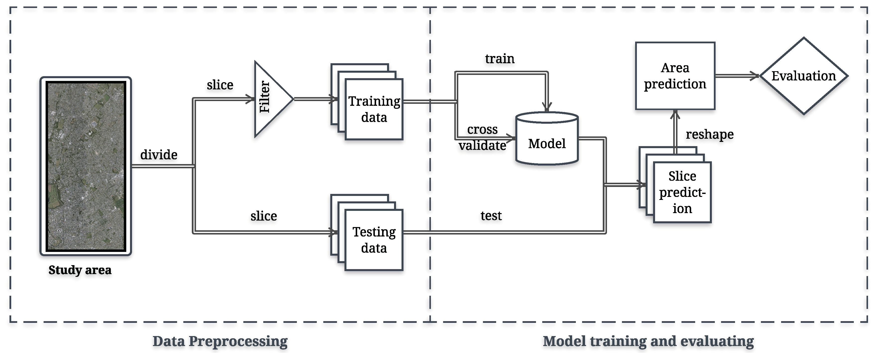
2.2.1. Data Preprocessing

The aerial imagery from the study area is divided into training and testing regions. Later, the aerial imagery from both regions is processed by a sliding window of 224 × 224 pixels (with stride of 224 pixels) to generate image slices. In deep learning, particularly for classification tasks, biased data typically leads to overfitting and poor generalization [42]. To avoid this issue, thresholding is applied to the slices generated from the training region to filter out image slices with low building coverage rates (e.g., building coverage rate ≤ 15%). After data preprocessing, the number of samples in training, validation and testing data are 27,912, 1952 and 71,688, respectively.

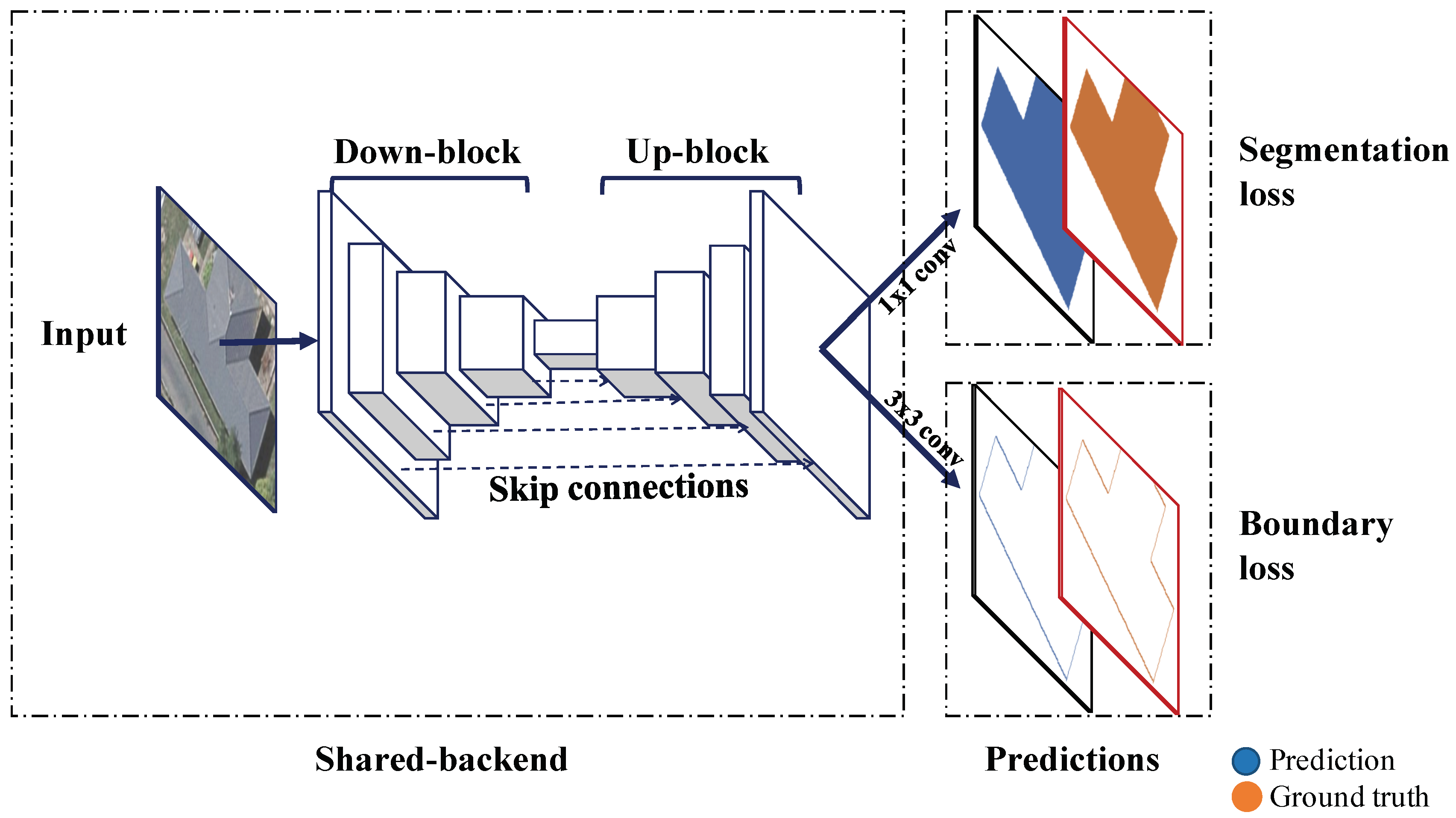
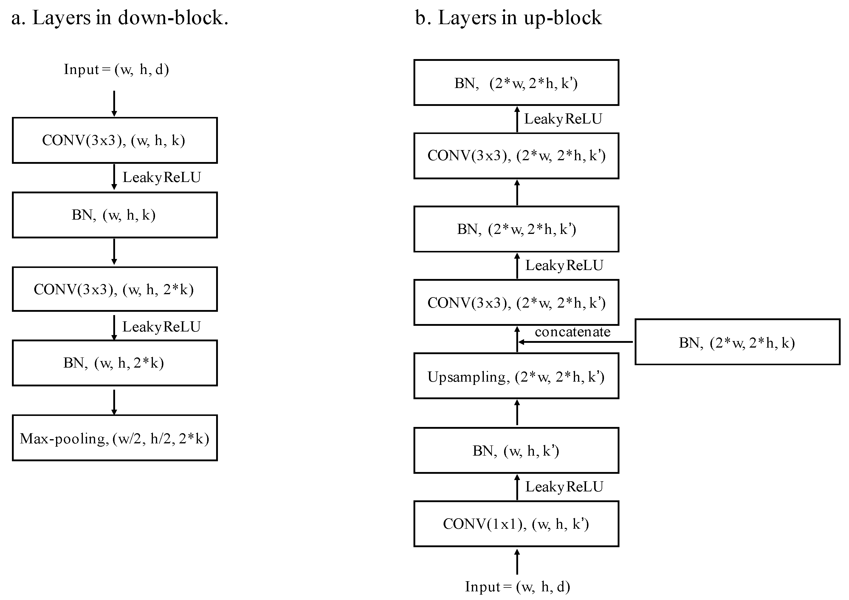
2.2.2. Boundary Regulated Network

The classic FCN model, which utilizes fully convolutional layers to perform pixel-to-pixel translations from inputs to outputs, is first proposed by Long et al. in 2015. By removing fully-connected layers, the FCN model greatly reduces the total number of parameters and significantly improves model performance. Advanced FCN-based models improve model performance by utilizing novel techniques, such as unsampling (SegNet), deconvolution (DenconvNet), skip connections (U-Net), and multi-constraints (MC-FCN). Although these FCN-based models are already very powerful, they still have some limitations:
  • For these models, the prediction value of each pixel is solely based on the features within a localized receptive field (e.g., a 3 × 3 kernel). Therefore, global information (e.g., linear relationships between points and right angle relationships between lines) of building polygons cannot be utilized by these models.
  • When capturing aerial imagery, it is inevitable to obtain noisy data, such as portions of buildings that are shadowed by surrounding trees. If the models are successfully trained to strictly segment the image solely by surrounding pixels, the hidden part of building polygon will be ignored.
To overcome these limitations, the proposed BR-Net model adopts multitask learning for segmentation and outline extraction to utilize both local and global information of images. During the training phase, the optimizer has two main tasks. It must ensure that both the segmentation and outline extraction prediction results are as consistent as possible with the corresponding ground truth. In this manner, during every iteration, the boundary information can restrict and regulate the parameter updating. It will prevent mapping pattern of model from biasing toward segmentation map of surrounding pixels.
Figure 3 presents the network architecture of the proposed BR-Net model. This model is composed of two parts: (1) an optimized U-Net-style FCN as a shared backend; and (2) a dual prediction framework for generating segmentation and outline extraction results. In the shared backend, there are several convolution, nonlinear activation, subsampling, and skip-connection operations.
The convolution operation is an element-wise multiplication performed via kernels. The size of the kernel determines the range of receptive field. In contrast to a rectified linear unit (ReLU) [43], which sets all values less than zero to zero, the output will be handled by a LeakyReLU with an alpha value of 0.1. To accelerate deep network training, avoid bias and prevent gradient vanishing, BN layers are heavily applied following convolutional layers. In this study, max-pooling [44] is chosen for subsampling the height and width of intermediate features. To achieve a consistent size between inputs and outputs, sequential bilinear upsampling [45] and skip-connection operations are implemented. A skip-connection is a concatenating operation across a single axis.
For multitask prediction, both segmentation and outline predictions are generated from the same output from the shared backend. For each prediction, a single kernel convolution operation followed by a sigmoid operation is required.
The binary cross entropy [46] between a prediction and the corresponding ground truth is utilized to compute the losses for segmentation ( L o s s s e g ) and outline ( L o s s b o u ). Each loss can be calculated as
L o s s = 1 h × w i = 1 , j = 1 h , w g i , j × log ( y i , j ) + ( 1 g i , j ) × log ( 1 y i , j )
where h and w represent the height and width of the prediction (y) and corresponding ground truth (g). The value of y i , j is the predicted probability of the pixel category.
Therefore, the total loss of the BR-Net can be formulated as
L o s s f i n a l = ( 1 α ) × L o s s s e g + α × L o s s b o u
where α is the weight of the boundary loss (Loss b o u ). In this study, the value of α is set to 0.5.
With final loss being minimized by an Adam optimizer [47] in every iteration, the BR-Net model learns a mapping pattern that can produce predictions for both segmentation and outlines utilizing a single input.

2.3. Experimental Setup

2.3.1. Architecture of the BR-Net

The architecture of the BR-Net consists of a shared backend and multitask prediction model. The shared backend consists of four sequential down-blocks, one central conv-block, and four sequential up-blocks. The central conv-block is a 3 × 3 convolutional layer with 384 kernels followed by a LeakyReLU activation function and BN layer. Four skip connections are placed between the 2nd BN layer among the down-blocks and corresponding upsampling layer among the up-blocks. The initial input of the model is an RGB image slice of 224 × 224 pixels. The output of each block serves as the input for the next block.
Figure 4a presents the structure of a down-block. The h, w, and d represent the height, width, and depth of an input, respectively. k represents the number of kernels that are utilized for convolution operations. Each down-block has two convolutional layers followed by two LeakyReLU activation functions, two BN layers, and a max-pooling layer. For each input, a down-block generates an output with half the width and height. The numbers of kernels in the four down-blocks are [24, 48, 96, 192].
Figure 4b presents the structure of an up-block. The h, w, and d represent the height, width and depth of an input, respectively. k and k’ represent the dimension of the corresponding BN layer among the down-blocks and the number of kernels utilized for convolution operations, respectively. In an up-block, there is a single bilinear upsampling layer, a skip connection layer, and three convolutional layers followed by LeakyReLU activation functions and BN layers. An up-block doubles the width and height of its input. The numbers of kernels in the four up-blocks are [192, 96, 48, 24].
The output of the shared backend is a 3D matrix with consistent width and height of the input image. A single 1 × 1 convolutional kernel followed by a sigmoid activation function is applied to the output to generate predictions for segmentation maps. Similarly, single 3 × 3 convolutional kernel with sigmoid activation function is used for generating outlines. The losses of different tasks are then calculated by computing the binary cross entropy between the predictions and ground truth.

2.3.2. Integration of Different Components

To further analyze the importance and significance of different components, including BN, LeakyReLU, and the proposed multitask training loss function, various combinations of the three components are tested in a comparison experiment. As shown in Table 1, BR-Net models with different combinations of components (with and without BN after each convolution operation, and with and without nonlinear activation of ReLU/LeakyReLU functions (see details in Figure 4)) are trained and validated utilizing the same training and testing data.

3. Results

The best FCN variant (FCN8s) and classic U-Net model are adopted as baseline models in our comparisons. These models, as well as the proposed BR-Net model, are trained and evaluated utilizing the same dataset and processing platform.

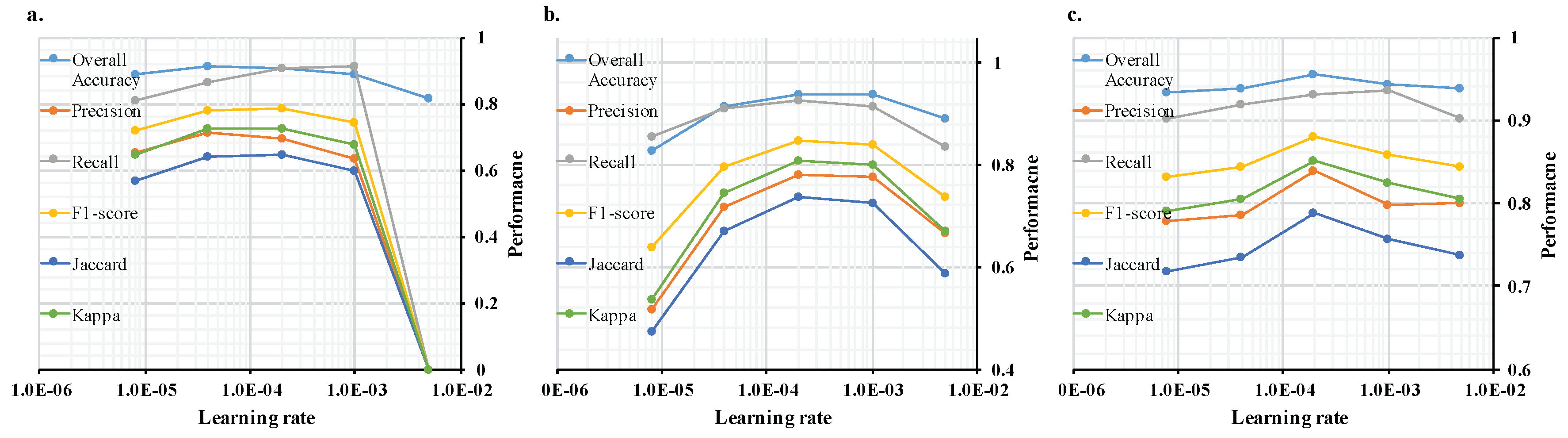
3.1. Hyper-Parameter Optimization

Figure 5 shows the trends of model performances under training rates of 5 × 10 3 , 1 × 10 3 , 2 × 10 4 , 4 × 10 5 and 8 × 10 6 . In general, too large (>1 × 10 3 ) or too small (<4 × 10 5 ) learning rate leads to poor performance. Three different methods (FCN8s, U-Net and BR-Net) show similar trends over various learning rates:
  • As shown in Figure 5a, FCN8s model achieves the best performance with the learning rate of 2 × 10 4 . For major metrics, FCN8s model shows similar values using learning rate between 4 × 10 5 and 2 × 10 4 .
  • As shown in Figure 5b, U-Net model shows the highest values of major metrics with the learning rate of 2 × 10 4 . Under learning rates from 2 × 10 4 to 1 × 10 3 , the performances of U-Net model are almost identical.
  • As shown in Figure 5c, similar to FCN8s and U-Net methods, the BR-Net model reaches its best performance with the learning rate of 2 × 10 4 .

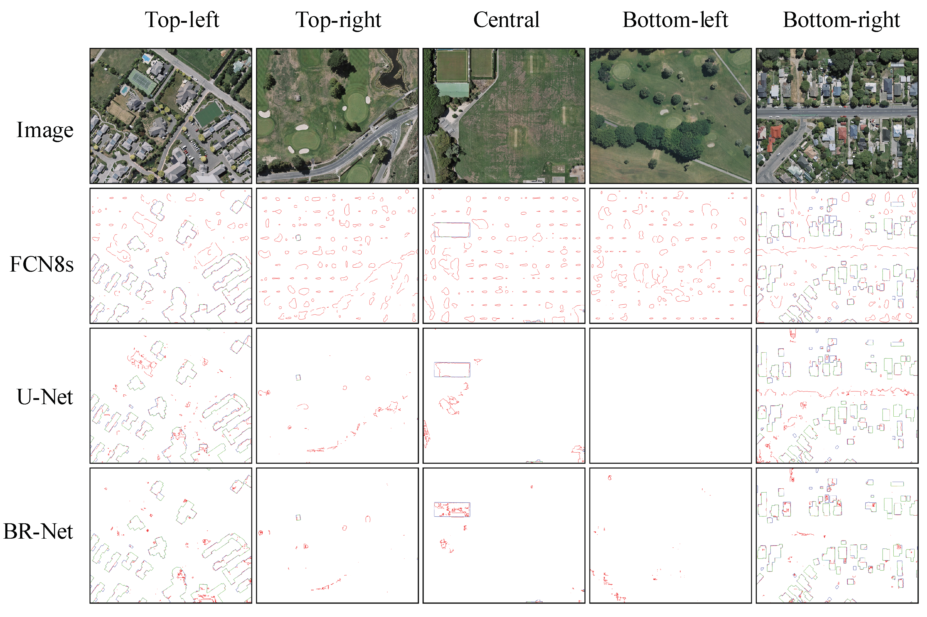
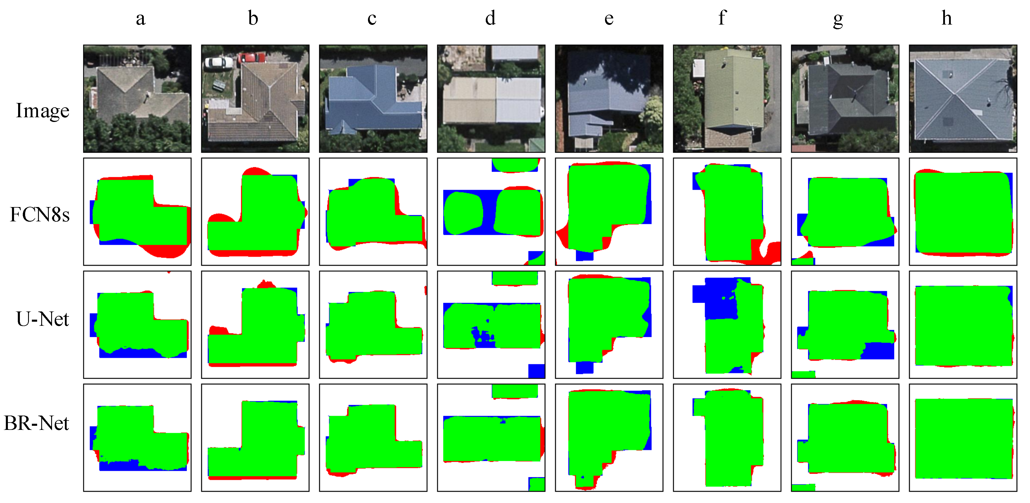
3.2. Qualitative Result Comparisons

3.2.1. Result Comparisons at Region Level

Figure 6 reveals that the BR-Net method is superior to U-Net and significantly outperformed the FCN8s method in the region-level comparison. In residential regions, such as the top-left and bottom-right regions, all three methods are capable of building recognition and segmentation. The FCN8s model presents significantly more false positives than the other methods. The U-Net model presents fewer false positives than FCN8s, but still failed to discriminate roads when compared to the BR-Net model. In non-residential regions, such as the top-right, central, and bottom-left regions, the U-Net and BR-Net models present a significantly smaller number of false positives than FCN8s.
Figure 7 presents the outline extraction results of the FCN8s, U-Net, and BR-Net methods. In residential regions (e.g., top-left and bottom-right regions), the majority of building outlines are extracted by all three models. However, the results from the FCN8s model contain more false positive polygons and lines compared to the other two methods. Compared to U-Net, BR-Net presents fewer false positives in adjacent areas between buildings and roads. Similar to the residential regions, in the non-residential regions in the top-right, central, and bottom-left portions of the test area, the FCN8s method generates a relatively large number of false positives.

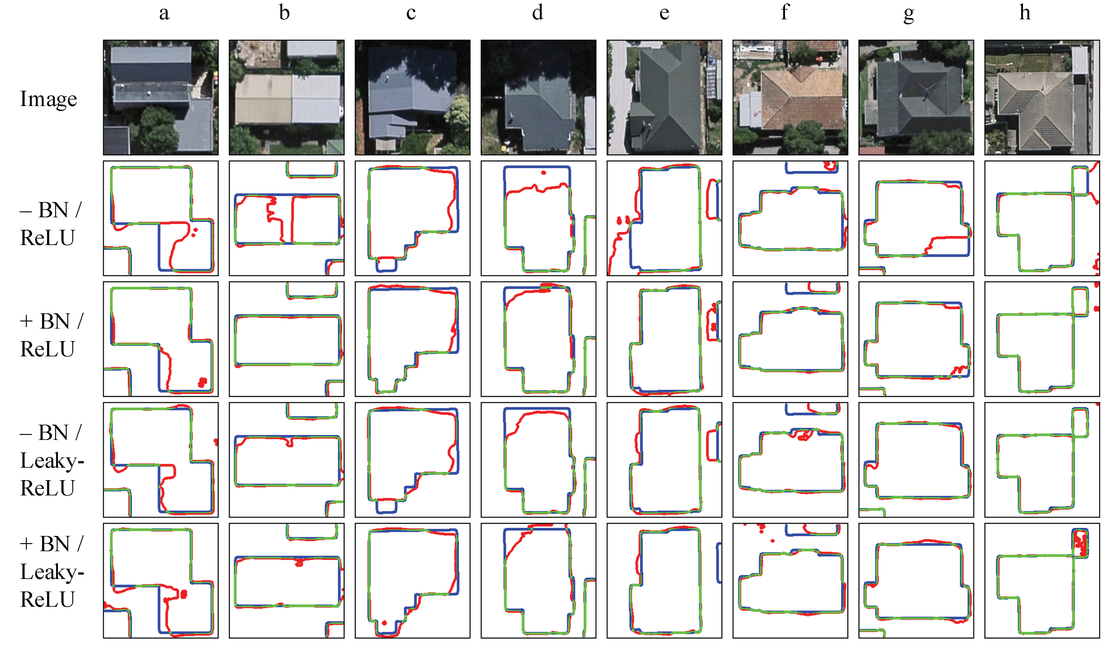
3.2.2. Result Comparisons at Single-House Level

To further explore the improvements in our method compared to other methods, several representative samples are selected for additional comparison.
Figure 8 presents eight representative groups of segmentation results generated by FCN8s, U-Net, and BR-Net. In general, U-Net and BR-Net perform better than FCN8s with slightly fewer false negatives (d and c) and significantly fewer false positives (a, b, e, f, and h), respectively. Compared to the U-Net model, BR-Net model generates fewer false negatives within buildings (a, d, f, and g) and fewer false positives around building edges (b, c, and e).
Figure 9 presents eight representative groups of outline extraction results from FCN8s, U-Net, and BR-Net. In general, all three methods can extract the major parts of buildings. For aerial images captured in good imaging conditions, both BR-Net and U-Net can generate near-perfectly aligned building outlines, whereas the polygon shapes in the FCN8s results are slightly twisted (c and h). For aerial images captured in shadowy condition, the BR-Net model produces results that are close to the actual shapes of buildings, instead of only the unobstructed parts of building (a, e, and g). It should be noted that, when both FCN8s and U-Net produce broken polygons, the proposed BR-Net model can still generate acceptable outlines (d and f).

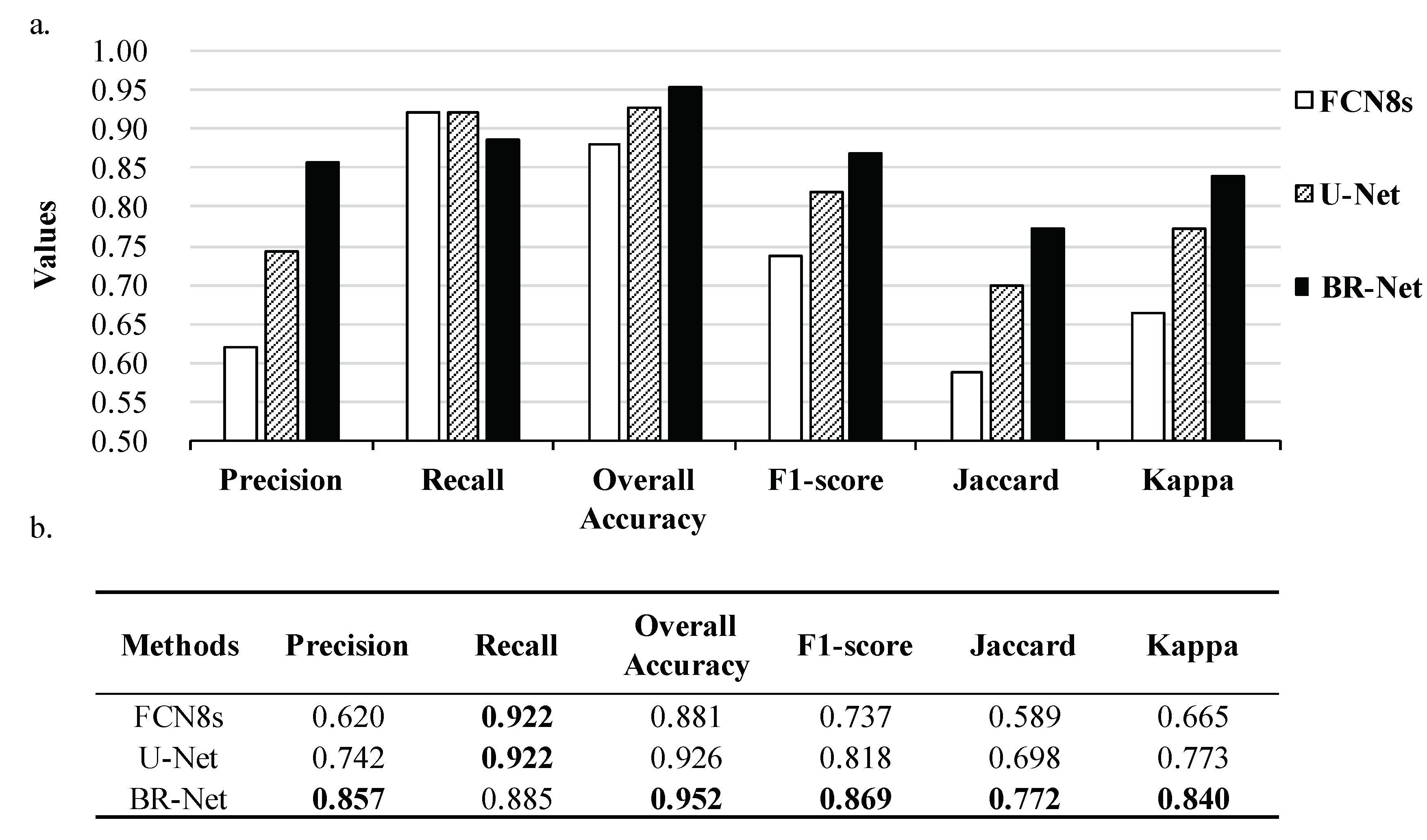
3.3. Quantitative Result Comparisons

In this study, two imbalanced metrics of precision and recall, and four general metrics of overall accuracy, F1 score, Jaccard index, and kappa coefficient are utilized for quantitative evaluations of roof segmentation results. Figure 10 presents comparative results between FCN8s, U-Net, BR-Net for the testing area.
For the imbalanced metrics of precision and recall, the BR-Net method achieves significantly higher values of precision (0.857 vs. 0.742 for U-Net and 0.620 for FCN8s), which indicates that our method performs well in terms of suppressing false positives. This result is consistent with the observations in Figure 6. However, compared to the recall value of 0.922 for FCN8s and U-Net, BR-Net achieves a slightly lower value of 0.885. Compared to the U-Net method, the BR-Net method shows 15.5% (0.857 vs. 0.742) improvement of precision and 4.0% (0.885 vs. 0.922) decline of recall. The improvement in precision (15.5%) significantly outweighs the decline in recall (4.0%).
For the four general metrics, the BR-Net model achieves the highest values for overall accuracy, F1 score, Jaccard index, and kappa coefficient. For overall accuracy, BR-Net achieves improvements of approximately 2.8% (0.952 vs. 0.926) over U-Net and 8.1% (0.952 vs. 0.881) over FCN8s. For F1 score, BR-Net achieves improvements of approximately 6.2% (0.869 vs. 0.818) over U-Net and 17.9% (0.869 vs. 0.737) over FCN8s. Compared to the FCN8s method, the BR-Net method achieves improvements of 30.1% (0.772 vs. 0.589) and 26.3% (0.840 vs. 0.665) for Jaccard index and kappa coefficient, respectively. Compared to the U-Net method, the BR-Net method achieves improvements of 10.6% (0.772 vs. 0.698) and 8.7% (0.840 vs. 0.773) for Jaccard index and kappa coefficient, respectively.

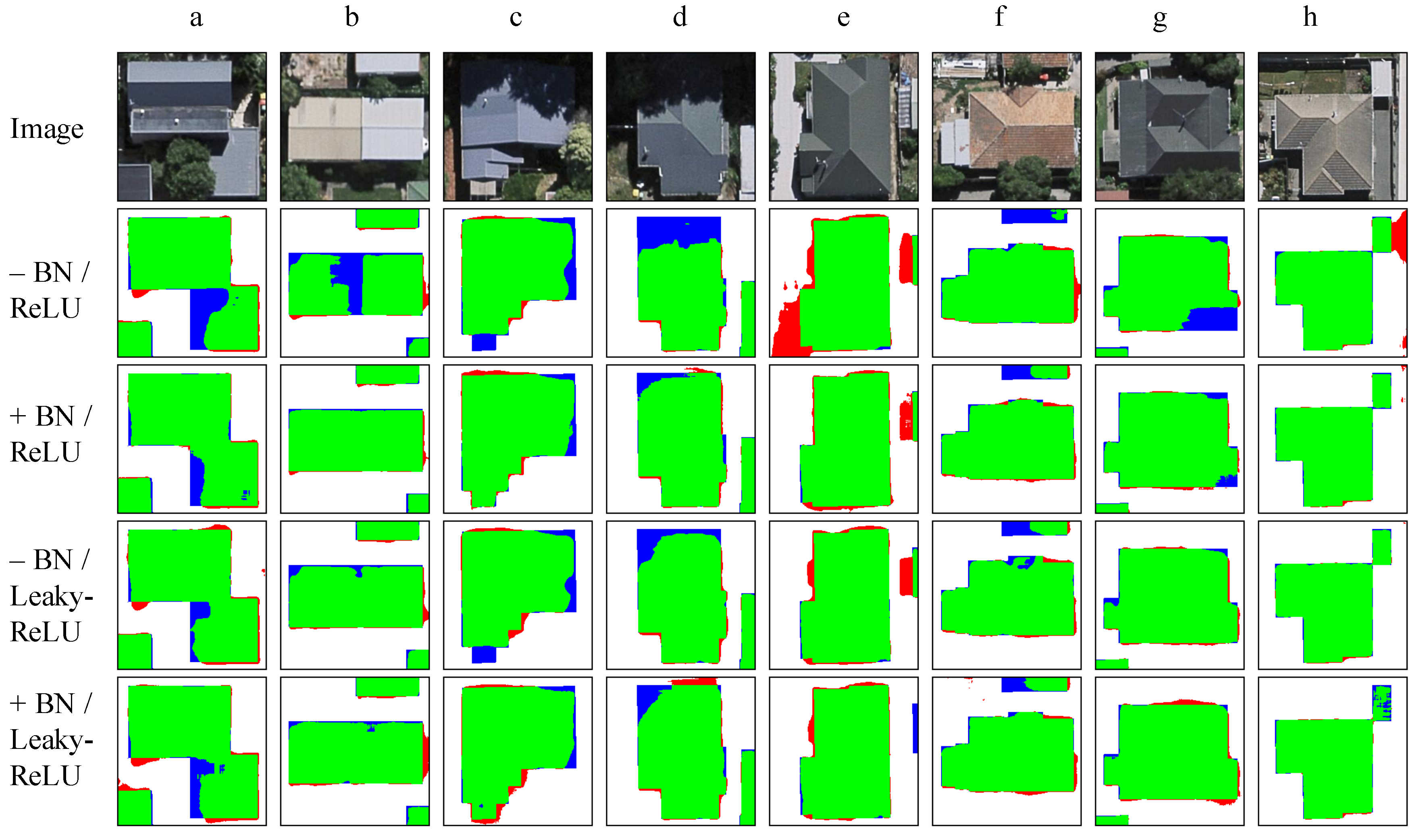
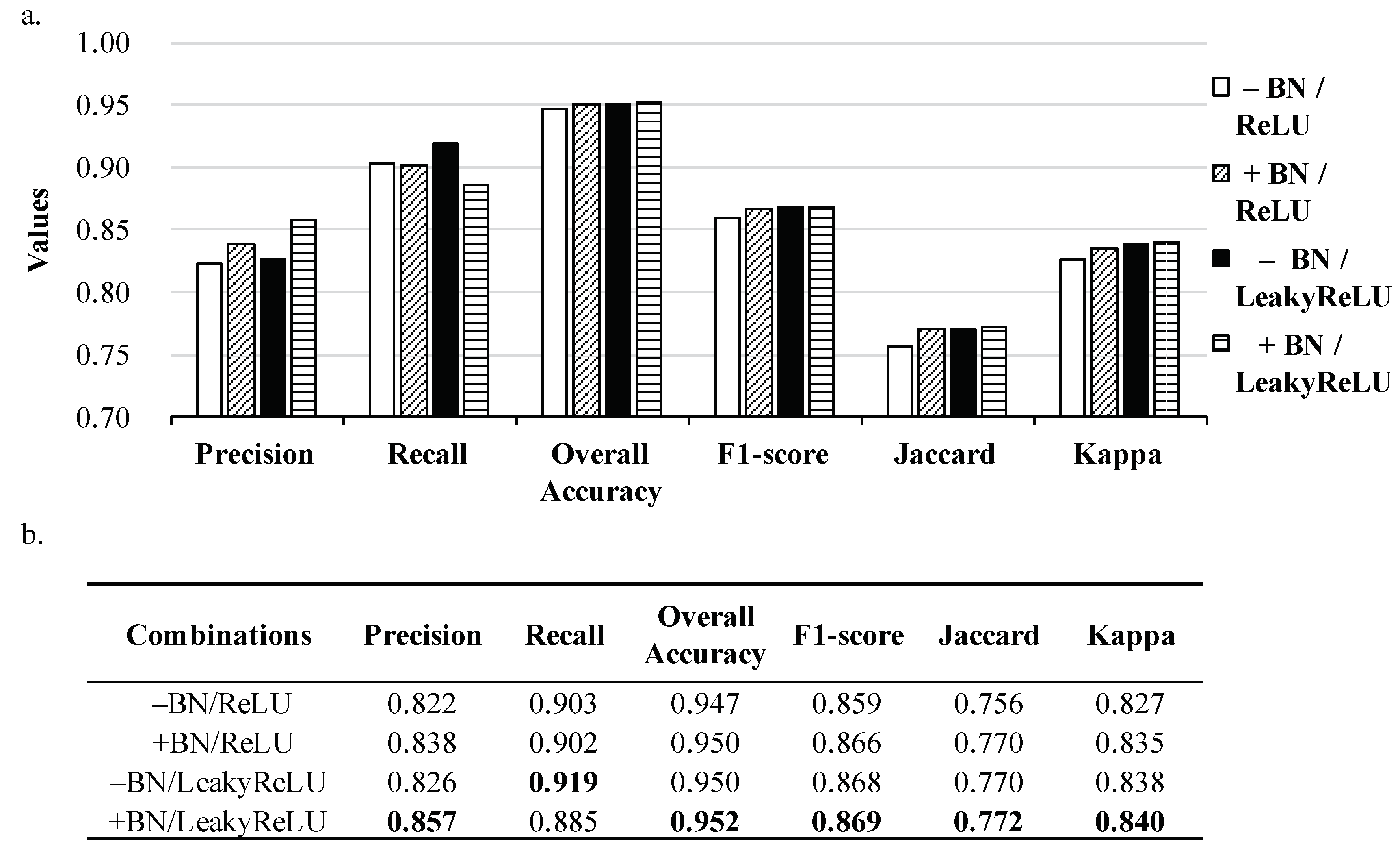
3.4. Sensitivity Analysis of Components

The sensitivity of the components for BN and nonlinear activation of ReLU/LeakyReLU functions is analyzed in this section.
Figure 11 presents representative roof segmentation results from BR-Net with different combinations of components. Compared to the basic BR-Net model (−BN/ReLU), adding BN (+BN/ReLU) or replacing the ReLU activation function with a LeakyReLU activation function (−BN/LeakyReLU), or combining both batch normalization and LeakyReLU (+BN/LeakyReLU) slightly reduces the number false positives (e and h) and false negatives (a, b, d, and g), which leads to better overall performance for roof segmentation. The performance improvements resulting from adding BN and replacing the activation function are quite similar.
Figure 12 presents representative results of single-house-level outline extraction from BR-Net with different combinations of components. Similar to the roof segmentation results, the BR-Net model with the addition of BN (+BN/ReLU) or replacement of the ReLU activation function with a LeakyReLU activation function (−BN/LeakyReLU), or combining both BN and LeakyReLU (+BN/LeakyReLU), produces better building contours for both shadowed (a, c, d, and g) and non-shadowed (b, e, f, and h) images. However, the differences between the BR-Net models of +BN/ReLU, −BN/LeakyReLU, and +BN/LeakyReLU are not significant.
The evaluation results of BR-Net with various combinations of components are presented in Figure 13.
In Figure 13a, for all evaluation metrics other than recall, the BR-Net model with the addition of BN (+BN/ReLU) or replacement of ReLU with LeakyReLU (−BN/LeakyReLU), or combining BN and LeakyReLU (+BN/LeakyReLU), produces slightly higher values than the basic model (−BN/ReLU). Compared to the basic model, the model utilizing LeakyReLU (−BN/LeakyReLU) produces a higher value of recall.
In Figure 13b, the BR-Net model with BN and LeakyReLU (+BN/LeakyReLU) produces the highest values for five out of six evaluation metrics, namely precision, overall accuracy, F1 score, Jaccard index, and kappa coefficient. Compared to the basic model, the increases in these metrics are 4.3% (0.857 vs. 0.822), 0.5% (0.952 vs. 0.947), 1.2% (0.869 vs. 0.859), 2.1% (0.772 vs. 0.756), and 1.6% (0.840 vs. 0.827), respectively. However, the model with BN and LeakyReLU results in the lowest value of recall with a decrease of approximately 2.0% (0.885 vs. 0.903) compared to the base model.

3.5. Computational Efficiency

The FCN8s, U-Net, and BR-Net models were implemented in PyTorch (https://pytorch.org/) and tested on a 64-bit Ubuntu system equipped with an NVIDIA GeForce GTX 1070 GPU (https://www.nvidia.com/en-us/geforce/products/10series/geforce-gtx-1070-ti/) and 8 GB of memory. During training, the Adam stochastic optimizer [47] with a learning rate of 2 × 10 4 and betas of (0.9, 0.999) was utilized. To conduct fair comparisons between the different methods, the batch size and iteration number for training were fixed as 24 and 10,000, respectively.
The computational efficiencies of the different methods during different stages are listed in Table 2. During the training stage, the FCN8s model processes approximately 29.3 frames per second (FPS), while the fastest model (U-Net) reached 91.7 FPS. For the BR-Net models, adding BN or replacing ReLU with LeakyReLU will decrease training speed. During the testing stage, as there is no need for gradient calculation or parameter updating, all models are 3–4 times faster. Similar to the training stage, the U-Net model is faster than all BR-Net models. However, the differences in their computational efficiencies become smaller. Compared to the BR-Net model with the best performance (+BN/LeakyReLU), the U-Net model achieves 16.2% (91.7 vs. 80.2) and 12.3% (280.6 vs. 249.9) higher FPS during the training and testing stages, respectively.

4. Discussion

4.1. Regarding the Proposed BR-Net Model

In the field of remote sensing, deep CNN models are first applied to detecting buildings in rural area [48] or informal settlements [49]. Because of limitations in terms of heavy memory costs and low computational efficiency, these patch-based CNN models are not capable of performing roof segmentation over large areas. In 2016, Maggiori et al. first adopted an FCN for segmenting large-scale aerial images [50,51]. With the development of new computer vision algorithms, more advanced FCN-based models, such as SegNet, U-Net, and MC-FCN, have been introduced and optimized for roof segmentation tasks.
In this paper, we propose a novel boundary regulated network termed BR-Net to improve capability of roof segmentation and outline extraction through combination of both local and global information of images. Existing advanced FCN-based models enhance the performance of the classic FCN model by either focusing on replacing the simple bilinear upsampling operation with more information-preserving methods (e.g., unsampling in SegNet and deconvolution in DeconvNet) or making better usage of the feature representation capability of hidden layers (e.g., skip-connections in U-Net and multi-constraints in MC-FCN). In contrast to other advanced FCN-based models, the proposed BR-Net model adopts a shared backend utilizing a modified U-Net and a dual prediction framework for the generation of segmentation and outline extraction results. Because of the multitask learning, BR-Net can utilize both local information from surrounding pixels to segment buildings and global information from polygons to generate outline. Comparative results from the testing area demonstrated that the proposed BR-Net model further improves the capability of FCN-based methods (FCN8s and U-Net) and achieves state-of-the-art performance on this task. Additionally, other techniques, such as BN and LeakyReLU activation, can be easily integrated into BR-Net to achieve superior performance.

4.2. Accuracies, Uncertainties, and Limitations

Compared to classic FCNs (FCN8s) and the state-of-the-art fully convolutional model (U-Net), BR-Net achieved the highest values for five out of six evaluation metrics (precision, overall accuracy, F1 score, Jaccard index, and kappa coefficient). The BR-Net model achieves a value of 0.857 for the precision, whereas U-Net and FCN8s only achieve values of 0.742 and 0.620, respectively. However, BR-Net shows slightly lower recall than FCN8s and U-Net (0.885 of BR-Net vs. 0.922 of FCN8s and U-Net). The increment of the precision as well as the decline of recall from BR-Net might due to the regulation of boundary information that avoid making prediction solely by surrounding pixels. Since the improvement in precision significantly outweighs the decline in recall, the proposed BR-Net model is superior to FCN8s and U-Net at roof segmentation and outline extraction tasks.
From the sensitivity analysis of different components, adding BN after each convolutional operation or replacing the traditional ReLU activation function with a LeakyReLU or combining both BN and LeakyReLU is able to improve the performance of the basic BR-Net model (see details in Figure 13).
As shown in Table 3, compared to U-Net, even the basic BR-Net model (−BN/LeakyReLU) achieves higher values for all evaluation metrics other than recall. Adding boundary loss to U-Net leads to better performance (basic BR-Net vs. U-Net). In comparison to optimized BR-Net, negative BR-Net shows smaller values of major metrics including precision, overall accuracy, f1-score, Jaccard index and kappa (see Rows 4 and 5 of Table 3). Removing boundary loss from optimized BR-Net leads to weaker performance (negative BR-Net vs. optimized BR-Net). These results demonstrate that our proposed boundary loss is a critical factor for improving model performance.
During our computational efficiency analysis, we observed a significant increasing in computational cost when utilizing the multitask framework, BN, or LeakyReLU in the training stage. The differences in processing speed became much smaller in testing stage. This decrease in computational efficiency may become a problem when applying our method to very large datasets, such as automatic mappings of provinces or entire countries. Additionally, compared to the performances of FCN8s and U-Net, the performance of BR-Net is lower by approximately 4.0% (0.885 vs. 0.922) in terms of recall. The balance between precision and recall must be studied further. Additionally, even for the optimized BR-Net model, there is still a certain amount of false positives in its prediction results (see top-right and bottom-left regions in Figure 6), which prevents its further application for more precise outline extraction and vectorization.

5. Conclusions

In this paper, we propose a novel boundary regulated network for accurate roof segmentation and outline extraction from VHR aerial images. The proposed BR-Net model has the ability to perform automatic segmentation and outline extraction from RGB images. Its performance is verified through several experiments on a VHR dataset covering approximately 32 km 2 . With its unique design of boundary restriction and regulation, the proposed method achieved significantly better performance than FCN8s and U-Net. In comparison to U-Net, BR-Net achieved gains of 6.2% (0.869 vs. 0.818), 10.6% (0.772 vs. 0.698), and 8.7% (0.840 vs. 0.773) in F1 score, Jaccard index, and kappa coefficient, respectively. Sensitivity analysis demonstrated that adding BN or utilizing LeakyReLU, or combining BN and LeakyReLU, can further improve model performance. In future studies, we will further optimize our network architecture to achieve better performance with less computational cost.

Author Contributions

G.W., X.S. (Xiaowei Shao), and R.S. conceived and designed the experiments. G.W. performed the experiments. G.W., Z.G., and X.S. (Xiaowei Shao) analyzed the data. X.S. (Xiaodan Shi), Q.C., and Y.X. contributed reagents/materials/analysis/tools. G.W. wrote the paper. All authors read and approved the submitted manuscript.

Funding

This work was partially supported by the Japan Society for the Promotion of Science (JSPS) Grant (No. 16K18162); National Natural Science Foundation of China, Project Number 41601506; and China Postdoctoral Science Foundation, Project Number 2016M590730.

Acknowledgments

We would like to thank the National Topographic Office of New Zealand for kindly sharing their data.

Conflicts of Interest

The authors declare no conflict of interest.

Abbreviations

The following abbreviations are used in this manuscript:
CNNConvolutional Neural Network
BNBatch Normalization
ReLURectified Linear Unit
FCNFully Convolutional Networks
FPSFrames Per Second
BR-NetBoundary Regulated Network

References

  1. Ma, L.; Li, M.; Ma, X.; Cheng, L.; Du, P.; Liu, Y. A review of supervised object-based land-cover image classification. ISPRS J. Photogramm. Remote Sens. 2017, 130, 277–293. [Google Scholar] [CrossRef]
  2. Li, M.; Zang, S.; Zhang, B.; Li, S.; Wu, C. A review of remote sensing image classification techniques: The role of spatio-contextual information. Eur. J. Remote Sens. 2014, 47, 389–411. [Google Scholar] [CrossRef]
  3. Chen, R.; Li, X.; Li, J. Object-based features for house detection from rgb high-resolution images. Remote Sens. 2018, 10, 451. [Google Scholar] [CrossRef]
  4. Xu, B.; Jiang, W.; Shan, J.; Zhang, J.; Li, L. Investigation on the weighted ransac approaches for building roof plane segmentation from lidar point clouds. Remote Sens. 2016, 8, 5. [Google Scholar] [CrossRef]
  5. Huang, Y.; Zhuo, L.; Tao, H.; Shi, Q.; Liu, K. A novel building type classification scheme based on integrated LiDAR and high-resolution images. Remote Sens. 2017, 9, 679. [Google Scholar] [CrossRef]
  6. Gilani, S.A.N.; Awrangjeb, M.; Lu, G. An automatic building extraction and regularisation technique using lidar point cloud data and orthoimage. Remote Sens. 2016, 8, 258. [Google Scholar] [CrossRef]
  7. Sahoo, P.K.; Soltani, S.; Wong, A.K. A survey of thresholding techniques. Comput. Vis. Graph. Image Process. 1988, 41, 233–260. [Google Scholar] [CrossRef]
  8. Kanopoulos, N.; Vasanthavada, N.; Baker, R.L. Design of an image edge detection filter using the Sobel operator. IEEE J. Solid-State Circuits 1988, 23, 358–367. [Google Scholar] [CrossRef]
  9. Wu, Z.; Leahy, R. An optimal graph theoretic approach to data clustering: Theory and its application to image segmentation. IEEE Trans. Pattern Anal. Mach. Intell. 1993, 15, 1101–1113. [Google Scholar] [CrossRef]
  10. Tremeau, A.; Borel, N. A region growing and merging algorithm to color segmentation. Pattern Recognit. 1997, 30, 1191–1203. [Google Scholar] [CrossRef]
  11. Gómez-Moreno, H.; Maldonado-Bascón, S.; López-Ferreras, F. Edge detection in noisy images using the support vector machines. In International Work-Conference on Artificial Neural Networks; Springer: Berlin/Heidelberg, Germany, 2001; pp. 685–692. [Google Scholar]
  12. Zhou, J.; Chan, K.; Chong, V.; Krishnan, S.M. Extraction of Brain Tumor from MR Images Using One-Class Support Vector Machine. In Proceedings of the 2005 IEEE 7th Annual International Conference of the Engineering in Medicine and Biology Society (EMBS 2005), Shanghai, China, 17–18 January 2006; pp. 6411–6414. [Google Scholar]
  13. Xie, S.; Tu, Z. Holistically-Nested Edge Detection. In Proceedings of the IEEE International Conference on Computer Vision, Santiago, Chile, 13–16 December 2015; pp. 1395–1403. [Google Scholar]
  14. Viola, P.; Jones, M. Rapid Object Detection Using a Boosted Cascade of Simple Features. In Proceedings of the 2001 IEEE Computer Society Conference on Computer Vision and Pattern Recognition (CVPR 2001), Kauai, HI, USA, 8–14 December 2001; Volume 1, p. I. [Google Scholar]
  15. Lowe, D.G. Object Recognition from Local Scale-Invariant Features. In Proceedings of the Seventh IEEE International Conference on Computer Vision, Kerkyra, Greece, 20–27 September 1999; Volume 2, pp. 1150–1157. [Google Scholar]
  16. Ojala, T.; Pietikainen, M.; Maenpaa, T. Multiresolution gray-scale and rotation invariant texture classification with local binary patterns. IEEE Trans. Pattern Anal. Mach. Intell. 2002, 24, 971–987. [Google Scholar] [CrossRef] [Green Version]
  17. Dalal, N.; Triggs, B. Histograms of Oriented Gradients for Human Detection. In Proceedings of the 2005 IEEE Computer Society Conference on Computer Vision and Pattern Recognition (CVPR 2005), San Diego, CA, USA, 20–25 June 2005; Volume 1, pp. 886–893. [Google Scholar]
  18. Inglada, J. Automatic recognition of man-made objects in high resolution optical remote sensing images by SVM classification of geometric image features. ISPRS J. Photogramm. Remote Sens. 2007, 62, 236–248. [Google Scholar] [CrossRef]
  19. Aytekin, Ö.; Zöngür, U.; Halici, U. Texture-based airport runway detection. IEEE Geosci. Remote Sens. Lett. 2013, 10, 471–475. [Google Scholar] [CrossRef]
  20. Dong, Y.; Du, B.; Zhang, L. Target detection based on random forest metric learning. IEEE J. Sel. Top. Appl. Earth Obs. Remote Sens. 2015, 8, 1830–1838. [Google Scholar] [CrossRef]
  21. LeCun, Y.; Bengio, Y. Convolutional networks for images, speech, and time series. Handb. Brain Theory Neural Netw. 1995, 3361, 1995. [Google Scholar]
  22. Ciresan, D.; Giusti, A.; Gambardella, L.M.; Schmidhuber, J. Deep neural networks segment neuronal membranes in electron microscopy images. In Proceedings of the Advances in Neural Information Processing Systems, Lake Tahoe, NV, USA, 3–6 December 2012; pp. 2843–2851. [Google Scholar]
  23. Krizhevsky, A.; Sutskever, I.; Hinton, G.E. Imagenet classification with deep convolutional neural networks. Proceedings of Advances in Neural Information Processing Systems, Lake Tahoe, NV, USA, 3–6 December 2012; pp. 1097–1105. [Google Scholar]
  24. Everingham, M.; Van Gool, L.; Williams, C.K.; Winn, J.; Zisserman, A. The pascal visual object classes (voc) challenge. Int. J. Comput. Vis. 2010, 88, 303–338. [Google Scholar] [CrossRef]
  25. Lin, T.Y.; Maire, M.; Belongie, S.; Hays, J.; Perona, P.; Ramanan, D.; Dollár, P.; Zitnick, C.L. Microsoft coco: Common objects in context. In European Conference on Computer Vision; Springer: Cham, Switzerland, 2014; pp. 740–755. [Google Scholar]
  26. Deng, J.; Dong, W.; Socher, R.; Li, L.J.; Li, K.; Li, F.-F. Imagenet: A Large-Scale Hierarchical Image Database. In Proceedings of the 2009 IEEE Conference on Computer Vision and Pattern Recognition (CVPR 2009), Miami, FL, USA, 20–25 June 2009; pp. 248–255. [Google Scholar]
  27. Guo, Z.; Shao, X.; Xu, Y.; Miyazaki, H.; Ohira, W.; Shibasaki, R. Identification of village building via Google Earth images and supervised machine learning methods. Remote Sens. 2016, 8, 271. [Google Scholar] [CrossRef]
  28. Long, J.; Shelhamer, E.; Darrell, T. Fully Convolutional Networks for Semantic Segmentation. In Proceedings of the IEEE Conference on Computer Vision and Pattern Recognition, Boston, MA, USA, 7–12 June 2015; pp. 3431–3440. [Google Scholar]
  29. Kampffmeyer, M.; Salberg, A.B.; Jenssen, R. Semantic Segmentation of Small Objects and Modeling of Uncertainty in Urban Remote Sensing Images Using Deep Convolutional Neural Networks. In Proceedings of the IEEE Conference on Computer Vision and Pattern Recognition Workshops, Las Vegas, NV, USA, 26 June–1 July 2016; pp. 1–9. [Google Scholar]
  30. Badrinarayanan, V.; Kendall, A.; Cipolla, R. Segnet: A deep convolutional encoder-decoder architecture for image segmentation. IEEE Trans. Pattern Anal. Mach. Intell. 2017, 39, 2481–2495. [Google Scholar] [CrossRef] [PubMed]
  31. Noh, H.; Hong, S.; Han, B. Learning Deconvolution Network for Semantic Segmentation. In Proceedings of the IEEE International Conference on Computer Vision, Santiago, Chile, 13–16 December 2015; pp. 1520–1528. [Google Scholar]
  32. Ronneberger, O.; Fischer, P.; Brox, T. U–Net: Convolutional networks for biomedical image segmentation. In International Conference on Medical Image Computing and Computer-Assisted Intervention; Springer: Cham, Switherland, 2015; pp. 234–241. [Google Scholar]
  33. Lin, T.Y.; Dollár, P.; Girshick, R.; He, K.; Hariharan, B.; Belongie, S. Feature pyramid networks for object detection. CVPR 2017, 1, 4. [Google Scholar]
  34. Wu, G.; Shao, X.; Guo, Z.; Chen, Q.; Yuan, W.; Shi, X.; Xu, Y.; Shibasaki, R. Automatic Building Segmentation of Aerial Imagery Using Multi-Constraint Fully Convolutional Networks. Remote Sens. 2018, 10, 407. [Google Scholar] [CrossRef]
  35. Polak, M.; Zhang, H.; Pi, M. An evaluation metric for image segmentation of multiple objects. Image Vis. Comput. 2009, 27, 1223–1227. [Google Scholar] [CrossRef]
  36. Carletta, J. Assessing agreement on classification tasks: The kappa statistic. Comput. Linguist. 1996, 22, 249–254. [Google Scholar]
  37. Ioffe, S.; Szegedy, C. Batch Normalization: Accelerating Deep Network Training by Reducing Internal Covariate Shift. In Proceedings of the International Conference on Machine Learning, Lille, France, 6–11 July 2015; pp. 448–456. [Google Scholar]
  38. Maas, A.L.; Hannun, A.Y.; Ng, A.Y. Rectifier nonlinearities improve neural network acoustic models. In Proceedings of the 30th International Conference on Machine Learning, Atlanta, GA, USA, 16–21 June 2013; Volume 30, p. 3. [Google Scholar]
  39. Li, E.; Femiani, J.; Xu, S.; Zhang, X.; Wonka, P. Robust rooftop extraction from visible band images using higher order CRF. IEEE Trans. Geosci. Remote Sens. 2015, 53, 4483–4495. [Google Scholar] [CrossRef]
  40. Plaza, A.; Martínez, P.; Pérez, R.; Plaza, J. Spatial/spectral endmember extraction by multidimensional morphological operations. IEEE Trans. Geosci. Remote Sens. 2002, 40, 2025–2041. [Google Scholar] [CrossRef]
  41. Canny, J. A computational approach to edge detection. In Readings in Computer Vision; Elsevier: New York, NY, USA, 1987; pp. 184–203. [Google Scholar]
  42. Goodfellow, I.; Bengio, Y.; Courville, A.; Bengio, Y. Deep Learning; MIT Press: Cambridge, MA, USA, 2016; Volume 1. [Google Scholar]
  43. Nair, V.; Hinton, G.E. Rectified Linear Units Improve Restricted Boltzmann Machines. In Proceedings of the 27th International Conference on Machine Learning (ICML-10), Haifa, Israel, 21–24 June 2010; pp. 807–814. [Google Scholar]
  44. Nagi, J.; Ducatelle, F.; Di Caro, G.A.; Cireşan, D.; Meier, U.; Giusti, A.; Nagi, F.; Schmidhuber, J.; Gambardella, L.M. Max-Pooling Convolutional Neural Networks for Vision-Based Hand Gesture Recognition. In Proceedings of the 2011 IEEE International Conference on Signal and Image Processing Applications (ICSIPA), Kuala Lumpur, Malaysia, 16–18 November 2011; pp. 342–347. [Google Scholar]
  45. Novak, K. Rectification of digital imagery. Photogramm. Eng. Remote Sens. 1992, 58, 339–344. [Google Scholar]
  46. Shore, J.; Johnson, R. Properties of cross-entropy minimization. IEEE Trans. Inf. Theory 1981, 27, 472–482. [Google Scholar] [CrossRef] [Green Version]
  47. Kingma, D.P.; Ba, J. Adam: A method for stochastic optimization. arXiv, 2014; arXiv:1412.6980. [Google Scholar]
  48. Guo, Z.; Chen, Q.; Wu, G.; Xu, Y.; Shibasaki, R.; Shao, X. Village Building Identification Based on Ensemble Convolutional Neural Networks. Sensors 2017, 17, 2487. [Google Scholar] [CrossRef] [PubMed]
  49. Mboga, N.; Persello, C.; Bergado, J.R.; Stein, A. Detection of Informal Settlements from VHR Images Using Convolutional Neural Networks. Remote Sens. 2017, 9, 1106. [Google Scholar] [CrossRef]
  50. Maggiori, E.; Tarabalka, Y.; Charpiat, G.; Alliez, P. Convolutional neural networks for large-scale remote-sensing image classification. IEEE Trans. Geosci. Remote Sens. 2017, 55, 645–657. [Google Scholar] [CrossRef]
  51. Maggiori, E.; Tarabalka, Y.; Charpiat, G.; Alliez, P. Fully Convolutional Networkss for Remote Sensing Image Classification. In Proceedings of the 2016 IEEE International on Geoscience and Remote Sensing Symposium (IGARSS), Beijing, China, 10–15 July 2016; pp. 5071–5074. [Google Scholar]
Figure 1. Aerial imagery of the study area ranging from 172 33 E to 172 40 E and 43 30 S to 43 32 S.
Remotesensing 10 01195 g001
Figure 2. Workflow for our study. The proposed BR-Net method is trained and cross validated utilizing the training data. Later, evaluation of model performance is conducted by utilizing the testing data.
Remotesensing 10 01195 g002
Figure 3. The network architecture of the proposed BR-Net model. The BR-Net model adopts a modified U-Net structure as a shared backend and performs multitask predictions for roof segmentation and outline extraction.
Remotesensing 10 01195 g003
Figure 4. Layers in down-blocks and up-blocks of the shared backend.
Remotesensing 10 01195 g004
Figure 5. Model performances using learning rates of 5 × 10 3 , 1 × 10 3 , 2 × 10 4 , 4 × 10 5 and 8 × 10 6 : (a) performances of FCN8s under various learning rates; (b) performances of U-Net under various learning rates; and (c) performances of BR-Net under various learning rates.
Remotesensing 10 01195 g005
Figure 6. Results of roof segmentation of regions by FCN8s, U-Net, and the proposed BR-Net. The five regions are located in the top-left, top-right, central, bottom-left, and bottom-right portions of the testing area. Each region contains 2240 × 2240 pixels. The green, red, blue, and white channels in the results represent true positive, false positive, false negative, and true negative predictions, respectively.
Remotesensing 10 01195 g006
Figure 7. Results of outline extraction from different regions by FCN8s, U-Net, and the proposed BR-Net. The five regions are located in the top-left, top-right, central, bottom-left, and bottom-right portions of the testing area. Each region contains 2240 × 2240 pixels. The green, red, blue, and white channels in the results represent true positive, false positive, false negative, and true negative predictions, respectively.
Remotesensing 10 01195 g007
Figure 8. Representative results of single-building-level segmentation by FCN8s, U-Net, and BR-Net. The green, red, blue, and white channels in the results represent true positive, false positive, false negative, and true negative predictions, respectively.
Remotesensing 10 01195 g008
Figure 9. Representative results of single-building-level outline extraction by FCN8s, U-Net and, BR-Net. The green, red, blue, and white channels in the results represent true positive, false positive, false negative, and true negative predictions, respectively.
Remotesensing 10 01195 g009
Figure 10. Comparison of segmentation performances of FCN8s, U-Net, and BR-Net across the entire testing area. (a) Bar chart for performance comparison. The x- and y-axis represent the evaluation metrics and corresponding values, respectively. (b) Table of performance comparisons of methods. For each evaluation metric, the highest values are highlighted in bold.
Remotesensing 10 01195 g010
Figure 11. Representative results of single-building-level roof segmentation from BR-Net with various combinations of components. The green, red, blue, and white channels in the results represent true positive, false positive, false negative, and true negative predictions, respectively.
Remotesensing 10 01195 g011
Figure 12. Representative results of single-building-level outline extraction from BR-Net with various combinations of components. The green, red, blue, and white channels in the results represent true positive, false positive, false negative, and true negative predictions, respectively.
Remotesensing 10 01195 g012
Figure 13. Comparison of segmentation performances of BR-Net models with various combinations of components. (a) Bar chart for performance comparison. The x- and y-axis represent the evaluation metrics and corresponding values, respectively. (b) Table of performance comparisons of methods. For each evaluation metric, the highest values are highlighted in bold.
Remotesensing 10 01195 g013
Table 1. Component combinations of BR-Net models.
CombinationsBNReLULeakyReLU
– BN / ReLU *
+ BN / ReLU**
– BN / LeakyReLU *
+ BN / LeakyReLU* *
Table 2. Comparison of computational efficiency of FCN8s, U-Net, and BR-Net with various combinations of components.
StageFCN8sU-NetBR-Net
(−BN/ReLU)
BR-Net
(+BN/ReLU)
BR-Net
(−BN/LeakyReLU)
BR-Net
(+BN/LeakyReLU)
Training (FPS)29.391.788.180.286.678.9
Testing (FPS)130.2280.6276.5252.5274.1249.9
Table 3. Comparison of segmentation performances of U-Net, basic BR-Net, negative BR-Net and optimized BR-Net. The highest values for different metrics are highlighted in bold.
MethodsPrecisionRecallOverall
Accuracy
F1-scoreJaccardKappa
U-Net0.7420.9220.9260.8180.6980.773
basic BR-Net 10.8220.9030.9470.8590.7560.827
negative BR-Net 20.7680.9510.9360.8450.7390.806
optimized BR-Net 30.8570.8850.9520.8690.7720.840
1 BR-Net (−BN/ReLU); 2 BR-Net (+BN/LeakyReLU), without boundary loss; 3 BR-Net (+BN/LeakyReLU).

