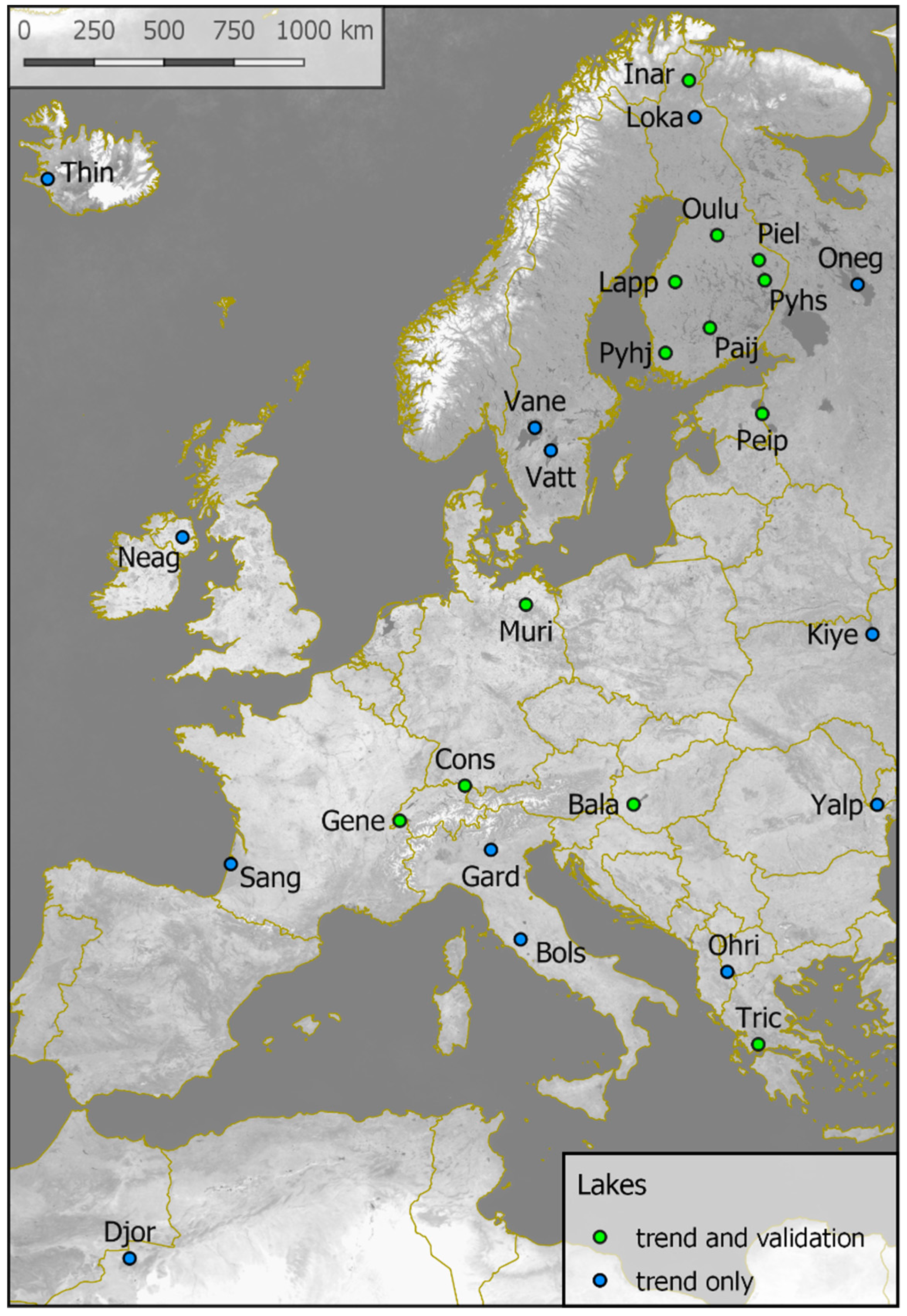
Article

Lake Surface Water Temperature Derived from 35 Years of AVHRR Sensor Data for European Lakes

by
Gian Lieberherr
1,2,* and
Stefan Wunderle
1,2
1
Institute of Geography, University of Bern, Hallerstrasse 12, CH-3012 Bern, Switzerland
2
Oeschger Centre for Climate Change Research, University of Bern, Falkenplatz 16, CH-3012 Bern, Switzerland
*
Author to whom correspondence should be addressed.
Remote Sens. 2018, 10(7), 990; https://doi.org/10.3390/rs10070990
Submission received: 14 May 2018 / Revised: 13 June 2018 / Accepted: 18 June 2018 / Published: 22 June 2018
(This article belongs to the Special Issue Satellite Remote Sensing for Water Resources in a Changing Climate)

Abstract

:
Lake surface water temperature (LSWT) is an important parameter with which to assess aquatic ecosystems and to study the lake’s response to climate change. The AVHRR archive of the University of Bern offers great potential to derive consistent LSWT data suited for the study of climate change and lake dynamics. To derive such a dataset, challenges such as orbit drift correction, non-water pixel detection, and homogenization had to be solved. The result is a dataset covering over 3.5 decades of spatial LSWT data for 26 European lakes. The validation against in-situ temperature data at 19 locations showed an uncertainty between ±0.8 K and ±2.0 K (standard deviation), depending on locations of the lakes. The long-term robustness of the dataset was confirmed by comparing in-situ and satellite derived temperature trends, which showed no significant difference. The final trend analysis showed significant LSWT warming trends at all locations (0.2 K/decade to 0.8 K/decade). A gradient of increasing trends from south-west to north-east of Europe was revealed. The strong intra-annual variability of trends indicates that single seasonal trends do not well represent the response of a lake to climate change, e.g., autumn trends are dominant in the north of Europe, whereas winter trends are dominant in the south. Intra-lake variability of trends indicates that trends at single in-situ stations do not necessarily represent the lake’s response. The LSWT dataset generated for this study gives some new and interesting insights into the response of European lakes to climate change during the last 36 years (1981–2016).

Graphical Abstract

1. Introduction

Water temperature is an important parameter within aquatic ecosystems. The metabolic rate of organisms and the activity of bacteria and algae is governed by water temperature [1,2,3,4]. Changing water temperature can alter the balance and the species composition of an aquatic ecosystem and even alter its trophic state [5,6,7]. Lake dynamic processes such as thermal stratification and mixing dynamics are firmly related to water temperatures [8,9]. The energy balance of large lakes is dominated by heat exchange processes at the surface [8]. Lake surface water temperature (LSWT) governs energy and mass exchange between the water body and the troposphere. It is also an important parameter in mesoscale meteorology and local climate models [10,11,12]. LSWT can be seen as an indicator of regional climate change [13], and several recent publications analyzed climate signals within lakes by investigating LSWT trends [14,15,16,17]. Recognizing its importance, LSWT was also added to the list of essential climate variables (ECV) by the Global Climate Observing System (GCOS), which needs to be monitored [18].
Traditionally, measurement of water temperature is done with in-situ thermometers, either manually or with automatic recording stations. Depending on the objectives of organizations or institutes, measurements are taken at various point-locations, at various intervals, and at various depths. This leads to a high heterogeneity amongst available lake water temperatures data, preventing the composition of consistent time series to be analyzed in the frame of climate change studies. Also, for lake dynamic studies, the 1D point measurements from automatic in-situ stations are not well suited; data with spatial coverage would be more valuable.
Remotely sensed earth observation data from satellites has the potential to overcome these limitations. For the study of lake dynamic processes and climate change, the spatial and temporal homogeneity of a dataset is of crucial importance, whereas the accuracy of an individual point-measurement is secondary. Satellite observation does not provide highly accurate temperature measurement for a single point in space. It provides a grid of temperature measurements, each averaged over a certain portion (depending on the resolution) of the lake’s surface. It is also supposed to have higher uncertainties due to atmospheric disturbance. However, the potential of temporal and spatial coverage is unique, and therefore remotely sensed surface water temperature from satellites is a highly relevant topic in the scientific community.
Having the WMO definition of a climate period in mind, homogeneous time series covering more than 30 years would be necessary to be relevant for the study of climate change. The Advanced Very High Resolution Radiometer (AVHRR), mounted on various satellite platforms since 1981, offers the possibility to generate such a data set. In 1981, the first AVHRR sensor recording in two TIR bands was launched with the NOAA-7 platform. Since then, the AVHRR sensor was mounted on the platforms of the NOAA series (until NOAA-19), and after on the last MetOp series, operated by EUMETSAT. This leads to an archive of AVHRR data starting in June 1981 until today. This time series, which covers over 35 years, is unique in satellite-based remote sensing, and therefore, despite the moderate resolution and the noise rate, the almost antique AVHRR sensor is still of interest today.
For this study, we generated a LSWT dataset of European lakes covering 36 years from 1981 to 2016 considering AVHRR local area coverage (LAC) data, archived at University of Bern, with a spatial resolution of 1.1 km in nadir. This data allows one to gain a unique insight into the response of European lakes to climate change in the last 3.5 decades.
The next chapter gives an overview of data and study sites considering 26 lakes distributed in Europe; in Section 3, the processing method is described in detail, which includes also post-processing based on different quality indicators and a correction of the diurnal temperature cycle to minimize the influence of orbit drift. Section 4 describes the results of this study, including validation with in-situ measurements and, finally, shows the trends for European lakes. The discussion in Section 5 compares the findings of LSWT trends with air temperatures of different periods and shows the influence of the measurement site on the trend. Section 6 concludes the paper.

2. Data and Study Sites

2.1. The Study Site

Lakes in and around Europe were selected to have a good distribution from east to west and from north to south (Figure 1). Only lakes exceeding a certain size were retained, because multiple adjacent water-only pixels must be available to perform accurate LSWT retrieval. In the case of the AVHRR sensor with a pixel size of roughly 1 km, this means that a lake should contain patches with open waters exceeding 3 × 3 km. For validation purposes, lakes with suitable in-situ temperature measurements also had to be among the selected lakes, in which ‘suitable’ means that the measurement should be representative of the open surface waters of the lake in terms of location and measurement depth.
With these criterions, a preselection adapted from Politi et al. [19] was used first, followed by a final manual selection. This led to a selection of 26 lakes (Table 1), with latitudes reaching from 31.53°N (Djorf Torba reservoir in Algeria) to 69.04°N (Inarijärvi in Finnland), and longitudes from 21.13°W (Thingvallavatn in Iceland) to 61.90°E (Lake Onega in the Russian Federation). The exact locations, where the LSWT data was resampled for the final time series, are shown in Table The sampling points were preferentially placed in the middle of large undisturbed open water surfaces, as the priority was to get the best possible conditions for an accurate measurement. Whereas, for the validation with in-situ data, sometimes different locations within the lakes were chosen (Table 2) to be as close as possible to the in-situ measurement location. These validation points were therefore often close to the shores, which had the effect of decreasing the availability and reliability of the satellite data while increasing the comparability with the in-situ measurements.

2.2. The Data

The AVHRR data archive from the University of Bern [20] was used to retrieve LSWT time series. The archive contains around 130,000 scenes from the European subset (Figure 1) and includes data from all NOAA and MetOp satellites with an AVHRR-2 or AVHRR-3 sensor on board (Figure 2). The data in the archive was preprocessed (see [20] for details) and included a probability cloud mask after Musial et al. [21] for each scene. The data of NOAA-15 was omitted, because the data from this platform showed significantly increased amounts of erroneous pixels and scanlines. The data from MetOp-1 was also omitted due to inconsistencies during the pre-processing.
The in-situ data available for this study is shown in Table 3 are, mainly, two types of measurements: homogeneous averaged measurements on a daily or hourly basis, and sporadic instant measurements at a defined point in time. For the measurements at lake Trichonida and Lake Balaton (Keszthely old), only the date (day) without exact timestamp (hh:mm) was available; therefore 12:00 local time was assumed. All the measurements are representing bulk temperatures close to the surface (taken at 0.1–1.0 m). Further, most of the northern lakes are ice covered during a certain amount of time per year. For these lakes, the amount of data per year (N/Yr. in Table 2) is considerably below of the expected 365 measurements (daily averaged data) per year.
The in-situ data were filtered for outliers and physically inconsistent values, as well as checked for irregularities such as systematic temperature changes due to modification of the equipment or the location. In the case of the INRA (Institute Nationale de la Recherche Agronomique) measurement at Lake Geneva, a systematic temperature decrease of roughly 0.4 °C was detected after autumn 2007, probably due to a dislocation of the station. Therefore, only the data from 1991 to 2007 from the INRA station was used.
It is assumed that the best validation performance will result from comparison with the hourly averaged and instant measurements, whereas for the daily measurements, the error between an individual satellite measurement and the daily average temperature can theoretically be as high as the amplitude of the diurnal temperature cycle.

3. Method

3.1. LSWT Processing Chain

Figure 3 shows a scheme of the main LSWT retrieval and processing steps performed for this study. For accurate LSWT retrievals, also the pre- and post-processing of the satellite data is very important, e.g., only reliable clear sky observations with accurate geocoding should be retained to ensure that the resulting temperatures correspond to the features we actually investigate. Conservative cloud and land masking are responsible for the elimination of non-water pixels. Parameters like view angles and spatial consistency of LSWT are additional indicators for the quality and reliability of the measurements. All this information is retained in a quality mask associated with the final LSWT product.
The pre-processing of the AVHRR data used for this study is described in Hüsler et al. [20] and provides georeferenced AVHRR scenes, as well as the associated cloud mask after Musial et al. [21]. The coefficients used for this study are time-independent and lake-specific coefficients, empirically matched to radiative transfer model results as described in Lieberherr et al. [22]. The details of the final LSWT retrieval is described within the following subchapters.

3.1.1. Georeferencing Test

Even on well geocoded AVHRR scenes, the accuracy of the geolocation can vary within the same scene. Thus, an additional georeferencing test was added to the pre-processing described in Hüsler et al. [20]. During the extractions of the sub-sets from the scene, an algorithm verifies and adjusts the local geocoding for each target location. The test is basically an edge detection and matching algorithm. First, an edge detection with a Laplace filter is applied to the subset of the scene, and to the subset of a reference image. Then, the correlation for each possible positioning of the AVHRR subset within the reference subset is computed, resulting in a correlation map. In the case of a correct georeferenced image, a correlation peak is found in the center of the correlation map. Otherwise, depending on the position of the correlation peak, a latitude and/or longitude shift is performed before the subset of the lake is extracted. To determine if the correlation maximum corresponds to the correct location, it is tested if the correlation peak is unique and of significant amplitude. The geolocation check is performed with AVHRR Band 2 data for daytime scenes, and with AVHRR Band 4 data for night-time scenes.

3.1.2. The LSWT Retrieval

A state-of-the-art split-window method was used to retrieve surface water temperature for this study. The idea is to make use of the different absorption characteristics of water vapor within differential spectral windows of the thermal infrared [23]. Two algorithms are currently used in various applications: the Multichannel Sea Surface Temperature (MCSST) algorithm [24] assumes a linear relationship between the atmospheric transmittance of the signal and the difference in absorption of the two channels. In contrast, the Non-Linear Sea Surface Temperature (NLSST) algorithm introduced in 1990 for NOAA SST products takes the nonlinear nature of atmospheric absorption into account, which increases the accuracy especially for daytime measurements [25,26]. Recent publications show no significant improvement when using the NLSST instead of the MCSST for LSWT retrieval [27,28,29]. Therefore, here the MCSST approach described by Equation (1) with empirically determined split window coefficients is used to derive LSWT from AVHRR data.
LSWT = a 0 + a 1 B T 4 + a 2 ( B T 4 B T 5 ) + a 3 ( 1 sec θ ) ( B T 4 B T 5 )
  • a 0 , 1 , 2 , 3 Split-window coefficients
  • B T 4 , 5 Brightness temperature from AVHRR band 4 and 5
  • θ Satellite view zenith angle
The coefficients where derived for each location (lake specific) and satellite, based on the findings of Lieberherr et al. [22]. It was assumed that the use of matchup data from a 2-year period is sufficient to obtain the infinite temporal validity of the coefficients. The used matchup data was generated with a radiative transfer model, RTTOV-11 [30], using atmospheric profiles of water vapor and temperature from the ERA-INTERIM [31] dataset.

3.1.3. Non-Water Pixels Elimination

Cloud and land masking is crucial for satellite-based temperature retrievals of surface lake water. Clouds are opaque to thermal infrared radiation, and even a slightly cloud-contaminated signal (sub-pixel sized clouds) can result in a considerably colder measurement of the temperature. Also, for land contaminated pixels, the signal can be biased, as the land surface temperature sometimes differs by several degrees from the water temperature. Therefore, strict cloud and land masking are necessary to eliminate affected pixels. On the other hand, this reduces the amount of available data to be used for further processing. An ideal cloud and land masking would eliminate all affected pixels without any false positives. As, of course, this is not feasible, a good trade-off tailored to the application must be found. For the cloud detection within this study, the probability cloud mask developed by [21] is used. Additionally, in order to improve the performance over inland-waterbodies and during night-time, some additional tests are performed. These additional tests are described in [32]. The masking of land pixels is done by applying a land-water mask (LWM).
The LWM is derived from freely available Open Street Map (OSM) data, which was found to be more accurate in geolocation than several other land classification datasets. The accuracy of OSM data was the subject of various studies, e.g., [33] reported an accuracy of ±3 m (SD) in an urban area in Germany, and [34] found an RMSE of 15 m in a remote rural area in Portugal. Further, the reliability of OSM data is considered good, since it is based on in-situ GPS measurements and is verified and reviewed by the OSM community. For easily accessible and frequently visited objects such as Lake Constance, the community is very active, and the data is highly reliable. When rasterizing the OSM-shapefile to the AVHRR pixel grid, the LWM is extended by 500 m (~1/2 pixel) into the lake to exclude lake pixels where the signal is potentially land contaminated. The low number of lakes (26) allowed us to check the thematic and geographic accuracy manually during the generation of the LWM raster files from the OSM water shapes.

3.1.4. Quality Levels

The reliability of each measurement (pixel) is expressed by a quality score reaching from Q0 to Q6; Table 3 recapitulates the six quality levels. The tests for the quality levels are cumulative, meaning that for each level, the tests of the previous quality levels have been passed too. Pixels with physically inconsistent values (LSWT > 35 °C or LSWT < −5 °C), as well as isolated pixels, are assigned to Q0; all other clear-sky pixels and water pixels are classified at least QPixels with a low spatial standard deviation (similarity to surrounding pixels) get QPixels outside the potential sun glint zone are assigned QQ4 and Q5 are achieved if the view zenith angle (VZA) is lower than 55° or 45°, respectively. Q6 is assigned if the georeferentiation is considered highly reliable. This means that during the georeferencing test, the feature (lake) must be detected with certainty. The results showed that at Q5 and Q6 (VZA < 45 and the enhanced georeferentiation test), the available pixels decrease strongly without considerably reducing the uncertainty. Finally, Q4 was used for the trend analysis during this study, as it was considered to be the best tradeoff between accuracy and data availability.

3.2. Time Series Generation

Once all the AVHRR scenes are processed, the 1D temperature timeseries for each specific target point are extracted from the 2D LSWT product. For each target point, pixels within a radius of 3 km are extracted. All invalid pixels and all pixels with a quality below the aimed quality level are removed. If at least 3 pixels remain within the 3 km radius around the target, the average of the valid pixels is retained. The thus-sampled temperature value is then integrated into the raw time series with the timestamp of the satellite scene accorded.
Before using this raw time series for validation and for trend analysis, an outlier detection adapted for such time-series is applied. The main problem with basic outlier detection on temperature time series is that the yearly and the diurnal temperature cycle already induces a high amount of variance in the data. For example, a measurement of 5 °C at Lake Constance in the middle of August should be detected as an outlier, as it is 10 °C to 20 °C below the expected temperature for August. However, since temperatures of 5 °C are usual in January, the measurement is not conspicuous when performing straightforward outlier detection. For robust outlier detection on a temperature time series, the known temperature cycles such as the yearly temperature cycle (YTC) must be removed first. In our case, this is done by computing the mean annual curve from the raw time series and then subtracting it from the respective values of the time-series. The YTC-corrected time series can then be analyzed. For the outlier detection, we have used a robust outlier detection method described in Leys et al. [35] using the mean absolute deviation and the median.
For the analysis of trends, the raw time series is not suitable, as neither the data density nor the overpass-time where the temperature is measured is stable through time. This can induce additional trends. In Figure 4, one can nicely see the evolving data density through the years: In the 1980s, only one satellite at the time was available, whereas in 2013 there were five. Also, the heterogeneity of overpass-times in general, as well as the shift in overpass time due to orbit drift of the individual satellites, can be also be seen in Figure 4.
To overcome the data density issue, monthly and seasonal averages of the YTC anomaly are computed. The YTC anomaly is computed with reference to lake-specific YTC issued form the whole period of available LSWT data (1981–2016). The averaging over months or seasons leads to a homogeneous distribution of the temperature data suited for trend analysis. By using the YTC anomaly instead of the LSWT, we aim at removing an eventual bias induced by uneven distribution of the measurements within the averaging period (month or season).
Finally, to solve the overpass-time problem, a diurnal temperature cycle (DTC) model was used to adjust each measurement to the daily mean temperature, as described in the following paragraphs.

3.3. Diurnal Temperature Cycle (DTC) Correction

The NOAA satellites are subject to relatively strong orbit drifts [36,37]. This means that through the years of operation, the overpass time at the same location is shifted. Figure 4 shows all scenes and recording times used during this study. One can see that the overpass time of each satellite changes over the years of operation, leading to shifts of over five hours. As lake surface water temperature is changing throughout a day, an overpass time at 1 p.m. would lead to higher average temperatures than an overpass time at 8 am. Therefore, drifting orbit leads to an artificial trend in long-time records when looking at only one platform. When it comes to time series over several platforms, as is the case here, the impact is hard to predict. Some authors claimed that the impact is negligible (e.g., [32]); others correct for the DTC (e.g., [38]).
For this study, we used a DTC correction based on the DTC model described in Equations (2)–(5) after Duan et al. [39]. The model was first developed by Inamdar et al. [40] for land surface temperature (LST) and tested against in-situ data with various land cover types, including water (Lake Tahoe). Duan et al. [39] improved the model by deducing the width ω (Equation (4)) over the half-period of the cosine term from the thermal diffusion equation. This model was successfully implemented and used for daytime LSWT retrieval by Pareeth et al. (e.g., [38]).
T s d ( t ) = T 0 + T a c o s ( π ω ( t t m ) ) ,     t < t s T s n ( t ) = T 0 + δ T + [ T a c o s ( u ) δ T ] k ( k + t t s ) ,     t t s
with
k = ω π [ t a n ( u ) 1 δ T T a   s i n ( u ) 1 ]
ω = 4 3 ( t m t s r )
u = π ω ( t s t m )
T s d and T s n are the day and night time surface temperatures, t is the time, T 0 the residual temperature at sunrise, T a is the temperature amplitude, δ T is the difference in temperature between T 0 and T ( t ) , ω is the width over the half-period of the cosine term, t s r is the sunrise time, t m is the time where daily maximum temperature is reached, t s is the time where free attenuation starts, and k is the attenuation constant.
During the here-presented study, instead of adjusting the satellite derived LSWT to a temperature equivalent of a standard acquisition time (12:00 UTC), we adjusted the temperature to the daily average temperature, computed from the modeled DTC curves. For each lake and for each month, typical DTC anomaly curves were computed by fitting the model to the available satellite LSWT data. The final LSWT was then adjusted to the daily average temperature by subtracting the temperature anomaly. The use of this approach improved the validation results within the here-presented study (see Section 4.2).

3.4. Trend Analysis

The linear trends were computed using the homogenized time series at the 26 locations (Table 1) described in the previous chapter. Non-parametric trend analysis was performed using the Thiel–Sen slope to quantify the trend and the Mann–Kendal test to determine its significance.
Several studies do compute only summer trends (e.g., [17]). This has the advantage of not having to deal with ice onset and breakup cycle. However, Winslow et al. [41] showed that seasonal trends such as a summer trend do not well represent the effects of climate change on the lakes. During this study, trends for all four seasons, as well as annual trends, were computed. When it comes to the definition of the seasons, there are mainly two ways described in literature: (1) summer defined as June, July, August (JJA), e.g., [42,43,44]; (2) summer defined as July, August, September (JAS), e.g., [17,32,41,45]. However, in the case of the lakes studied here, the influence of spring warming on the JJA period and the influence of fall cooling on the JAS period are disproportionately high (see Figure 5). We concluded that both JAS and JJA were not suitable for “summer only trend” in a restricted sense. For this study, we overcame this issue by taking the middle way; thus, the periods start and end in the middle of the months: Summer is defined as the period from 15 June to 14 September (JJAS), autumn as from 15 September to 14 December (SOND), winter from 15 December to 14 March (DJFM), and, finally, spring from 15 March to 14 June (MAMJ). Choosing these periods, the characteristics of the seasons are more pronounced (spring = warming, fall = cooling, summer = hot, and winter = cold) looking at the annual temperature cycle (Figure 5).

4. Results

4.1. Validation of Retrieved Lake Surface Water Temperature

The main performance indicator for the retrieval validation during this study is the standard deviation (SD), whereas the root mean square error (RMSE) and the bias are considered as secondary performance indicators. As we are primarily interested in temperature patterns such as temporal trends or spatial gradients, the uncertainty between two distinct measurements in time or space (SD) needs to be as small as possible, whereas the systematic part of the uncertainty (bias) is of lower importance. In fact, the bias affects all measurements in the same way, and therefore does not mask patterns such as spatial gradients and temporal trends. For the LSWT retrieval, the variable part of the uncertainty (SD) is mainly induced by variability in atmospheric composition, weather conditions, small-scale lake dynamic processes, and sensor noise, whereas the systematic part of the uncertainty (bias) is induced by factors such as skin-bulk temperature difference, in-situ sensor location, or sensor-related issues.
Further, it must be mentioned that during validation, we are comparing two measurements of a physical quantity against each other. This means that none of the two measurements (in-situ and satellite) do represent the truth to the full extent. This got even worse when considering the fact that they technically do not measure exactly the same quantity: The in-situ temperature measurement deduces the water temperature at a specific point in space (location and depth), whereas the satellite measurement estimates the temperature of the uppermost skin layer, averaged over a certain spatial extent, which is defined by its resolution. The exact amount of uncertainty issued from the described difference in measurement technique and measured quantity could not be determined during this study. Also, the correction methods for the skin to bulk difference as proposed by Donlon [46] or Minnet [47] for SST retrieval did not improve the validation performance: The method, applied to LSWT, only affects the systematic bias and has no effect on the variance of the error.
In Figure 6, one can see the difference when validating the same satellite data with data from two different in-situ locations close to each other. This relativizes the significance of such validation results, even though they still give a general indication about how well the retrieval works. However, it reminds us to be careful with the in-situ data, and to not take it as the finite truth.
Table 4 shows the validation results at all in-situ stations. There seem to be two main factors influencing the validation performance. First, there is the latitude, as it seems that with higher cloud cover rate and longer periods of ice cover during the cold season, also the quality of the retrieval decreases. On the other hand, the data type of the in-situ data seems to play an important role too: There are three types of in-situ data: daily averaged, hourly averaged, and manually taken instant measurements. The validation against instant and hourly averaged measurements yields the best results, as it allows for close temporal matchups between satellite overpass and in-situ measurements (matchup window ±1 h).
Amongst the instant measurements, the validation at Müritz yields the best results (SD ± 0.82 K, Figure 7a), but due to its sporadic sampling frequency only 66 matchups where available. The performance of the instant measurements at Lake Balaton (SD ± 1.44 K, Figure 7b) and Lake Trichonidas (SD ± 1.04 K) is lower, but at these locations the exact in-situ measurement timestamp was unknown. The validation with hourly averaged measurements has considerably higher number of matchups, and the performances reach from ±0.95 K (Lake Constance, Bregenz new, Figure 6a) to ±1.40 K (Lake Constance, Lindau, Figure 6b). The validation with daily averaged in-situ data shows, generally, a lower performance than with instant and hourly measurements. The SD reaches from very low ±1.07 K (Geneva, INRA Figure 8a) to rather increased values of ±2.05 K at Lake Inarijärvi (Figure 8b).

4.2. Validation of the DTC Correction and Trends

For the validation with daily in-situ data, the available satellite LSWT is compiled to daily average temperatures. To reduce the impact of the daily temperature cycle (DTC), a DTC correction is applied to the satellite retrievals. The validation with DTC-corrected data results in a decrease of SD by 0% to 15.6% depending on the lakes, and in an average decrease of 6% or 0.11 K, respectively (Table 5).
The trends from the in-situ stations with a period covered of at least 25 years were compared to the trends computed from LSWT retrievals. This was done for both the DTC-corrected satellite data and for the non-adjusted satellite data. Table 6 shows results from this comparison. At three of the six locations, the DTC adjusted trends are considerably closer to the in-situ trends (Inarijärvi, Lappajärvi, and Oulujärvi). At two locations (Pyhäselka and Peipsi), the DTC adjustment has almost no effect, and the LSWT trends remain close to the in-situ trends. At lake Pielinen, however, the DTC adjustment has a negative effect: the raw trend is in fact closer to the in-situ trend.

4.3. Trend Analysis

The yearly and seasonal trends at all studied locations are shown in Table 7. Only significant trends (Kendall p-value < 0.05) were retained for further analysis.
All annual trends where significant and positive, thus indicating a warming of the lakes water temperature (Table 7). The strongest annual warming trend is observed at Lake Onega with 0.76 K/dec, whereas the weakest trend is to be found at Djorf Torba Reservoir with 0.17 K/dec. The trend at Lake Onega is remarkable, as there is no similar trend within the studied lakes; the next highest trend is 0.54 K/dec for lake Pyhäjärvi. The trend at Djorf Torba has to be looked at with care, as there has been a strong siltation going on since the drought period in the 1990s: The volume loss was estimated at 35% in 2014, with the siltation still going on at a rate of 0.9% per year [48].
Figure 9 shows details of the temperature anomaly in annual resolution of lakes representing geographical extremes (N-S, W-E). The significance of a long time series including years from 1981 onwards is clearly shown with increased frequency of blue bars during the earlier years (1981–1995) in comparison to the latest years with higher temperatures. Especially the warm period of the last five years is obvious, independently of the geographical location of the lakes. However, these high temperatures are more pronounced in northern and eastern areas, whereas the lake in Iceland (Thingvallavatn) shows reduced temperature increase, probably due to the oceanic influence. Also, one of the southern lakes (Trichonida, Figure 9) shows a reduced increase of temperature, which is probably also influenced by the proximity to the Mediterranean Sea. In all studied lakes, we can identify spatial gradients of the magnitude of temperature trends: The trends are increasing from south (Lake Trichonida 0.21 K/decade, Figure 9a) to north (e.g., Inarijärvi 0.50 K/decade, Figure 9b), and also from west (e.g., Thingvallavatn 0.38 K/decade, Figure 9c) to east (e.g., Lake Onega 0.76 K/decade, Figure 9d). The gradient is strongest on the diagonal from the south-west to north-east, whereas the magnitude of the trends shows a significant correlation with the latitude (R2 = 58%, Figure 10a) and a rather weak correlation with longitude (R2 = 24%, Figure 10b).
When looking at the strongest seasonal trends in Table 7, one can see that at lower latitudes the winter trends and some spring trends are dominant. This is typically the case for the subalpine lakes such as Lake Geneva, Lake Garda, and Lake Constance, which all show dominant winter trends. When moving north, first the spring (e.g., Balaton, Müritz, and Vättern) and then the summer trends (e.g., Pyhäjärvi, Päijänne, and Onega) start to dominate. Finally, for the highest latitudes, the autumn trends are clearly dominating (all lakes north to Lake Onega).
Looking at the north–south gradient of the seasonal trends (Figure 11), we see that winter trends seem almost unaffected by the latitude in contrast to the other seasonal trends. Especially, autumn trends are very sensible to latitude: At low latitudes, temperature trends in autumn are less pronounced than winter or spring trends, whereas at northern latitudes they are the strongest seasonal trends.
The West–East gradient of the seasonal trends is less significant, and probably influenced by the transition from oceanic to continental climate. However, this could not be investigated in more detail with the available data.

5. Discussion

The validation shows that with careful processing, the difficulties related to the AVHRR sensor such as orbit drift and small georegistration errors and others could be overcome. The importance of the in-situ measurements has been emphasized during the validation, and it was shown that the quality of the in-situ measurement is significantly influencing the performance of the validation. This indicates that the satellite retrieval has reached an accuracy level at which more accurate in-situ measurements are needed to further assess the quality of the LSWT retrieval. Also, the derived trends could be well validated with the in-situ measurements.
Concerning the significance test of the trends, only significant trends (Kendal p-value < 0.05 Table 7) were retained for further analysis. In contrast to the yearly trends, not all seasonal trends fulfilled this criterion. In the case in which the Kendall p-value is above 0.05, there are two plausible interpretations: (1) There is a strong trend, but due to elevated variance in the data and/or due to short periods and low amount of data, the trend cannot be determined with confidence. With this, erroneous estimates of trends can be detected (e.g., winter trend at Lake Päijiänne Table 7); (2) There is no trend or a weak trend in the data, and the p-value is increased, because we are close to the null-hypothesis. In this case, we eliminate a potentially correct value of weak trend close to 0 K/decades such as winter and autumn trends from lake Sanguinet (Figure 12). Thus, it is important to emphasize that with the used method, we can detect significant trends, but we cannot detect trends near 0 K/decade with certitude. This explains the discrepancy when comparing the annual trend with the valid seasonal trends from Table 7, in which our intuition is that the average of the seasonal trends is more or less equal to the yearly trend.
Trends are sensitive to different factors such as the period in which a trend is determined, the homogenization of the data, and the type of trend (seasonal, yearly, etc.). Therefore, the comparison with trends from individual lakes in other studies is not meaningful. However, on the other hand, more general statements can be looked at in detail. For example, Schneider and Hook [17] mention elevated summer trends in Northern Europe of up to around 0.8 K/dec. Our results suggest the same tendency of stronger trends in north-east Europe, whereas the strongest trends are rather to be found in autumn than in summer. The approximatively 0.8 K/dec in summer is only reached in Lake Onega, whereas at Inarijärvi and at the Lokka Reservoir such elevated trends are occurring during autumn.
Another observation from Schneider and Hook [17], that lakes in Northern Europe are warming more rapidly than local air temperature, was confirmed (see e.g., Lake Vättern Figure 13a). According to our results, this phenomenon is not limited to northern Europe: it can also be observed at some lakes in central Europe such as Lake Constance (Figure 13b). However, the difference in trends between local air temperature and LSWT is reduced when moving south towards warmer lakes. Additionally, for Lake Bolsena (Figure 13c), the air temperature trend tends even to be more pronounced than the LSWT trends. However, the reasons for the strong LSWT trends compared to local air temperature were not further investigated here.
The seasonal trends we detected show a high intra-seasonal variability within the same lake (Table 7), and therefore we can state that none of the seasons are representative for the overall trend within a lake. This is perfectly aligned with the main statement of Winslow et al. [41], who claim that summer trends do not fully represent the effects of climate change on lake temperatures. When we compare the yearly temperature cycle deduced from the first and the last 15-year period of the dataset, we can observe that the temperature evolution is very heterogeneous over the year, and also very different from lake to lake. For example, at Lake Bolsena and Lake Constance (Figure 14a,b), we observe significant warming during winter and spring. However, then there are also some short periods in which the recent years were colder than the first years of the dataset (mid-summer at Lake Constance, end of summer and start of autumn at Lake Bolsena). In contrast to this, at Lake Vättern and Lake Onega (Figure 14c,d), a moderate to significant warming during the whole year is observed, whereas this is more pronounced in summer and autumn. Lake Onega shows a significantly earlier and more pronounced warming in spring and during summer, resulting in a remarkable summer temperature peak that is higher and earlier than in the first years of the dataset.
Further, also within the same water body, trends can change significantly. This result is in agreement with the results of [16], in which intra-lake heterogeneity of trends was studied in large lakes. At lake Peipus (Figure 15), the yearly trend in the open waters in the north indicates a warming of 0.24 K/decade, whereas the warming rate almost doubles (0.44 K/decade) within the narrower part of the lake around Mehikoorma, in which also an in-situ station is located. This shows that the location where the temperature is sampled has an impact on the resulting trends. However, the example at lake Peipus shows us also that trends computed with the data of an in-situ measurement taken at a specific location are not necessarily representative of the temperature trend of the entire lake.

6. Conclusions

During this study, we could show that the AVHRR LAC data (1 km) archive at University of Bern can be used to yield good quality LSWT of an exceptional long-time span of over 35 years. This offers the possibility to study lake dynamics related to climate change. The quality of the retrieved LSWT could be confirmed by validation considering in-situ measurements, but it could also be shown that the quality of the validation data is essential.
A homogeneous LSWT dataset from 26 European lakes covering the period from 1981 to 2016 was created. With this, we were able to compute LSWT trends and to compare average yearly temperature cycles of different periods, of different geographic locations.
For all locations, significant LSWT trends indicating a warming were found. A gradient of increasing warming trends was revealed when moving from the south-west to the north-east of Europe. Whereas winter trends are not significantly affected, autumn trends are very sensitive to the location of the lake, especially to the latitude. Looking at the dominant seasonal trends per lake, we observe a shift from stronger winter trends in the south to dominant autumn trends in northern lakes, passing by a mixture of strong spring and summer trends in-between.
Generally, the strong interannual heterogeneity of the trends was detected in all lakes, showing that using only a defined period of the year to determine the temperature trend is not representative. It could be confirmed that the different seasons contribute unequal to the yearly trends, and that trend analysis based on summer seasons only does not show the complete reality.
Also, intra-lake heterogeneity of trends was detected. The location of measurements influences the trend directly, implying that a one-to-one comparison of trends between in-situ and satellite data has to be handled with care. We could show that temperature trends computed with data from in-situ measurements from individual stations are not suited to represent trends of an entire lake. This emphasizes the importance of satellite-based lake monitoring, as it adds significantly to the understanding of the big picture.
The comparison with local air temperature trends showed that many lakes have a stronger warming rate than local air temperature. This effect was shown to be more significant in colder lakes and in higher latitudes, e.g., Lake Vättern shows a stronger increase of LSWT than air temperature, but for Lake Bolsena in Italy the LSWT trend is even slightly weaker than for local air temperature.
The dataset generated within this study will be further investigated, and it has the potential to reveal further findings about the effects of climate change on European lakes. An extension of the dataset to more lakes in Europe would also be of great use for further investigations, especially regarding the east–west gradient of temperature trends, for which evidence was found. Also, a closer look at the influence on temperature trends of morphologic parameters such as the average depth of lakes could be the topic of further investigations.
For an extension of the dataset to other lakes in Europe, the size of the lakes is the only limiting factor, whereas for an extension on a global scale, the availability of AVHRR LAC data would be limiting. The application of the method to more recent sensors with higher resolution would be interesting for lake dynamic studies, but it is limited to a more recent time-period due to the availability of adequate satellite data.
Using open street map data for the generation of the LWM (land water mask) worked well. However, in the case of a larger number of lakes, and when taking in account the changes in time of global surface water occurrence, a global water mapping dataset such as presented in Pekel et al. 2016 [49] could be a more robust alternative for the generation of the LWM.

Author Contributions

The idea was conceived by G.L. and refined by S.W. The software development and data processing were mainly conducted by G.L. Both authors contributed to the interpretation of the results and to the writing and preparation of the manuscript for publication.

Funding

This study was funded by the Swiss National Science Foundation (SNSF) (SNF No. 200021 146740). Swiss Space Office of the State Secretariat for Education, Research, and Innovation of the Swiss Confederation (SERI/SSO) partly contributed to the funding of this study in the frame of the Mesures de Positionnement project MusenAlp.

Acknowledgments

We are grateful to the Dundee Satellite Receiving Station for making the AVHRR data from 1981 to 1989 available as a contribution for ESAs Long Term Data Preservation Program. Additionally, special thanks goes to all the providers of in-situ temperatures data: Wasserwirtschaftsamt Kempten (Lindau, Lake Constance)—Abteilung Wasserwirtschaft, Land Vorarlberg (Bregenz, Lake Constance)—members of the École Polytechnique Fédérale de Lausanne (Buchillon, Lake Geneva)—Vera Istvánovics from MTA-BME Water Research Group, Hungarian Academy of Sciences (Keszthely, Lake Balaton)—Károly Kutics from Lake Balaton Research Institute, Kaposvár University (Siofok, Lake Balaton)—Institut National de la Recherche Agronomique (INRA, Lake Geneva)—Olli-Pekka Mattila from the Finish Environment Institute SYKE (all Finnish lakes)—Peeter and Tiina Nõges Centre for Limnology, Estonian University of Life Sciences (Mehikoorma, Lake Peipsi)—George Kehayias, Environmental and Natural Resources Management, University of Patras (Lake Trichonidas).

Conflicts of Interest

The authors declare no conflict of interest.

References

  1. Müren, U.; Berglund, J.; Samuelsson, K.; Andersson, A. Potential effects of elevated sea-water temperature on pelagic food webs. Hydrobiologia 2005, 545, 153–166. [Google Scholar] [CrossRef]
  2. Hoppe, H.G.; Breithaupt, P.; Walther, K.; Koppe, R.; Bleck, S.; Sommer, U.; Jürgens, K. Climate warming in winter affects the coupling between phytoplankton and bacteria during the spring bloom: A mesocosm study. Aquat. Microb. Ecol. 2008, 51, 105–115. [Google Scholar] [CrossRef]
  3. Wetzel, R.E. Limnology: Lake and River Ecosystems, 3rd ed.; Academic Press: San Diego, CA, USA, 2001. [Google Scholar]
  4. Bouffard, D.; Kiefer, I.; Wüest, A.; Wunderle, S.; Odermatt, D. Are surface temperature and chlorophyll in a large deep lake related? An analysis based on satellite observations in synergy with hydrodynamic modelling and in-situ data. Remote Sens. Environ. 2018, 209, 510–523. [Google Scholar] [CrossRef]
  5. Malmaeus, J.M.; Blenckner, T.; Markensten, H.; Persson, I. Lake phosphorus dynamics and climate warming: A mechanistic model approach. Ecol. Model. 2006, 190, 1–14. [Google Scholar] [CrossRef]
  6. Scheffer, M.; Straile, D.; Van Nes, E.H.; Hosper, H.; Nov, N. Climatic Warming Causes Regime Shifts in Lake Food Webs Climatic warming causes regime shifts in lake food webs. Limnol. Oceanogr. 2008, 46, 1780–1783. [Google Scholar] [CrossRef]
  7. Jeppesen, E.; Mehner, T.; Winfield, I.J.; Kangur, K.; Sarvala, J.; Gerdeaux, D.; Rask, M.; Malmquist, H.J.; Holmgren, K.; Volta, P.; et al. Impacts of climate warming on the long-term dynamics of key fish species in 24 European lakes. Hydrobiologia 2012, 694, 1–39. [Google Scholar] [CrossRef] [Green Version]
  8. Fink, G.; Schmid, M.; Wahl, B.; Wolf, T.; Wüest, A. Heat flux modifications related to climate-induced warming of large European lakes. Water Resour. Res. 2014, 50, 2072–2085. [Google Scholar] [CrossRef]
  9. Komatsu, E.; Fukushima, T.; Harasawa, H. A modeling approach to forecast the effect of long-term climate change on lake water quality. Ecol. Model. 2007, 209, 351–366. [Google Scholar] [CrossRef]
  10. Balsamo, G.; Salgado, R.; Dutra, E.; Boussetta, S.; Stockdale, T.; Potes, M. On the contribution of lakes in predicting near-surface temperature in a global weather forecasting model. Tellus Ser. A Dyn. Meteorol. Oceanogr. 2012, 64, 1–12. [Google Scholar] [CrossRef]
  11. Dutra, E.; Stepanenko, V.M.; Balsamo, G.; Viterbo, P.; Miranda, P.M.A.; Mironov, D.; Schär, C. An offline study of the impact of lakes on the performance of the ECMWF surface scheme. Boreal Environ. Res. 2010, 15, 100–112. [Google Scholar]
  12. Samuelsson, P.; Kourzeneva, E.; Mironov, D. The impact of lakes on the European climate as simulated by a regional climate model. Boreal Environ. Res. 2010, 15, 113–129. [Google Scholar]
  13. Adrian, R.; Reilly, C.M.O.; Zagarese, H.; Baines, S.B.; Hessen, D.O.; Keller, W.; Livingstone, D.M.; Sommaruga, R.; Straile, D.; Van Donk, E. Lakes as sentinels of climate change. Limnol. Oceanogr. 2009, 54, 2283–2297. [Google Scholar] [CrossRef] [PubMed] [Green Version]
  14. Pareeth, S.; Bresciani, M.; Buzzi, F.; Leoni, B.; Lepori, F.; Ludovisi, A.; Morabito, G.; Adrian, R.; Neteler, M.; Salmaso, N. Warming trends of perialpine lakes from homogenised time series of historical satellite and in-situ data. Sci. Total Environ. 2017, 578, 417–426. [Google Scholar] [CrossRef] [PubMed]
  15. O’Reilly, C.M.; Sharma, S.; Gray, D.K.; Hampton, S.E.; Read, J.S.; Rowley, R.J.; Schneider, P.; Lenters, J.D.; McIntyre, P.B.; Kraemer, B.M.; et al. Rapid and highly variable warming of lake surface waters around the globe. Geophys. Res. Lett. 2015, 42, 10773–10781. [Google Scholar] [CrossRef]
  16. Woolway, R.I.; Merchant, C.J. Intralake Heterogeneity of Thermal Responses to Climate Change: A Study of Large Northern Hemisphere Lakes. J. Geophys. Res. Atmos. 2018, 123, 3087–3098. [Google Scholar] [CrossRef]
  17. Schneider, P.; Hook, S.J. Space observations of inland water bodies show rapid surface warming since. Geophys. Res. Lett. 2010, 37, 1–5. [Google Scholar]
  18. GCOS. Implementation plan for the global observing system for climate in support of the UNFCCC. World Meteorol. Organ. 2010. [Google Scholar]
  19. Politi, E.; MacCallum, S.; Cutler, M.E.J.; Merchant, C.J.; Rowan, J.S.; Dawson, T.P. Selection of a network of large lakes and reservoirs suitable for global environmental change analysis using Earth Observation. Int. J. Remote Sens. 2016, 37, 3042–3060. [Google Scholar] [CrossRef] [Green Version]
  20. Hüsler, F.; Fontana, F.; Neuhaus, C.; Riffler, M.; Musial, J.; Wunderle, S. AVHRR Archive and Processing Facility at the University of Bern: A comprehensive 1-km satellite data set for climate change studies. EARSeL eProceedings 2011, 10, 83–101. [Google Scholar]
  21. Musial, J.P.; Hüsler, F.; Sütterlin, M.; Neuhaus, C.; Wunderle, S. Probabilistic approach to cloud and snow detection on Advanced Very High Resolution Radiometer (AVHRR) imagery. Atmos. Meas. Tech. 2014, 7, 799–822. [Google Scholar] [CrossRef] [Green Version]
  22. Lieberherr, G.; Riffler, M.; Wunderle, S. Performance Assessment of Tailored Split-Window Coefficients for the Retrieval of Lake Surface Water Temperature from AVHRR Satellite Data. Remote Sens. 2017, 9, 1334. [Google Scholar] [CrossRef]
  23. Anding, D.; Kauth, R. Estimation of sea surface temperature from space. Remote Sens. Environ. 1970, 1, 217–220. [Google Scholar] [CrossRef]
  24. McClain, E.P.; Pichel, W.G.; Walton, C.C. Comparative Performance of Avhrr-Based Multichannel Sea Surface Temperatures. J. Geophys. Res. 1985, 90, 11587–11601. [Google Scholar] [CrossRef]
  25. Walton, C.C. Nonlinear Multichannel Algorithms for Estimating Sea Surface Temperature with AVHRR Satellite Data. J. Appl. Meteorol. 1988, 27, 115–124. [Google Scholar] [CrossRef] [Green Version]
  26. Walton, C.C.; Pichel, W.G.; Sapper, J.F.; May, D.A. The development and operational application of nonlinear algorithms for the measurement of sea surface temperatures with the NOAA polar-orbiting environmental satellites. J. Geophys. Res. 1998, 103, 27999. [Google Scholar] [CrossRef]
  27. Hulley, G.C.; Hook, S.J.; Schneider, P. Optimized split-window coefficients for deriving surface temperatures from inland water bodies. Remote Sens. Environ. 2011, 115, 3758–3769. [Google Scholar] [CrossRef]
  28. Oesch, D.C.; Jaquet, J.-M.; Hauser, A.; Wunderle, S. Lake surface water temperature retrieval using advanced very high resolution radiometer and Moderate Resolution Imaging Spectroradiometer data: Validation and feasibility study. J. Geophys. Res. 2005, 110, 1–17. [Google Scholar] [CrossRef]
  29. Li, X.; Pichel, W.; Clemente-Colon, P.; Krasnopolsky, V.; Sapper, J. Validation of coastal sea and lake surface temperature measurements derived from NOAA/AVHRR data. Int. J. Remote Sens. 2001, 22, 1285–1303. [Google Scholar] [CrossRef] [Green Version]
  30. Saunders, R.; Hocking, J.; Rundle, D.; Rayer, P.; Matricardi, M.; Geer, A.; Lupu, C.; Brunel, P.; Vidot, J. Rttov-11 Science and Validation Report. 2013. Available online: https://www.nwpsaf.eu/site/download/documentation/rtm/docs_rttov11/rttov11_svr.pdf (accessed on 19 June 2018).
  31. Dee, D.P.; Uppala, S.M.; Simmons, A.J.; Berrisford, P.; Poli, P.; Kobayashi, S.; Andrae, U.; Balmaseda, M.A.; Balsamo, G.; Bauer, P.; et al. The ERA-Interim reanalysis: Configuration and performance of the data assimilation system. Q. J. R. Meteorol. Soc. 2011, 137, 553–597. [Google Scholar] [CrossRef]
  32. Riffler, M.; Lieberherr, G.; Wunderle, S. Lake surface water temperatures of European Alpine lakes (1989-2013) based on the Advanced Very High Resolution Radiometer (AVHRR) 1 km data set. Earth Syst. Sci. Data 2015, 7, 1–17. [Google Scholar] [CrossRef]
  33. Helbich, M.; Amelunxen, C.; Neis, P. Comparative Spatial Analysis of Positional Accuracy of OpenStreetMap and Proprietary Geodata. In GI_Forum 2012 Geovisualization, Society and Learning; Herbert Wichmann Verlag, VDE VERLAG GMBH: Berlin, Germany, 2012; pp. 24–33. [Google Scholar]
  34. Monteiro, E.V.; Fonte, C.C.; Lima, J.L.M.P. Assessing positional accuracy of drainage networks extracted from ASTER, SRTM and OpenStreetMap. In Proceedings of the 18th AGILE International Conference on Geographic Information Science, Lisboa, Portugal, 9–12 June 2015; pp. 1–5. [Google Scholar]
  35. Leys, C.; Ley, C.; Klein, O.; Bernard, P.; Licata, L. Detecting outliers: Do not use standard deviation around the mean, use absolute deviation around the median. J. Exp. Soc. Psychol. 2013, 49, 764–766. [Google Scholar] [CrossRef] [Green Version]
  36. Latifovic, R.; Pouliot, D.; Dillabaugh, C. Identification and correction of systematic error in NOAA AVHRR long-term satellite data record. Remote Sens. Environ. 2012, 127, 84–97. [Google Scholar] [CrossRef]
  37. Jin, M.; Treadon, R.E. Correcting the orbit drift effect on AVHRR land surface skin temperature measurements. Int. J. Remote Sens. 2003, 24, 4543–4558. [Google Scholar] [CrossRef]
  38. Pareeth, S.; Salmaso, N.; Adrian, R.; Neteler, M. Homogenised daily lake surface water temperature data generated from multiple satellite sensors: A long-term case study of a large sub-Alpine lake. Sci. Rep. 2016, 6, 31251. [Google Scholar] [CrossRef] [PubMed] [Green Version]
  39. Duan, S.; Li, Z.; Tang, B.-H.; Wu, H.; Tang, R.; Bi, Y.; Zhou, G. Estimation of Diurnal Cycle of Land Surface Temperature at High Temporal and Spatial Resolution from Clear-Sky MODIS Data. Remote Sens. 2014, 6, 3247–3262. [Google Scholar] [CrossRef] [Green Version]
  40. Inamdar, A.K.; French, A.; Hook, S.; Vaughan, G.; Luckett, W. Land surface temperature retrieval at high spatial and temporal resolutions over the southwestern United States. J. Geophys. Res. Atmos. 2008, 113. [Google Scholar] [CrossRef] [Green Version]
  41. Winslow, L.A.; Read, J.S.; Hansen, G.J.A.; Rose, K.C.; Robertson, D.M. Seasonality of change: Summer warming rates do not fully represent effects of climate change on lake temperatures. Limnol. Oceanogr. 2017, 62, 2168–2178. [Google Scholar] [CrossRef]
  42. Fiedler, E.E.K.; Martin, M.M.J.; Roberts-jones, J.; Fiedler, E.E.K.; Martin, M.M.J.; An, J.R. An operational analysis of lake surface water temperature. Tellus A 2014, 1, 1–13. [Google Scholar] [CrossRef] [Green Version]
  43. Balsamo, G.; Dutra, E.; Stepanenko, V.M.; Viterbo, P.; Miranda, P.M.A.; Mironov, D. Deriving an effective lake depth from satellite lake surface temperature data: A feasibility study with MODIS data. Boreal Environ. Res. 2010, 15, 178–190. [Google Scholar]
  44. Wahl, B.; Peeters, F. Effect of climatic changes on stratification and deep-water renewal in Lake Constance assessed by sensitivity studies with a 3D hydrodynamic model. Limnol. Oceanogr. 2014, 59, 1035–1052. [Google Scholar] [CrossRef] [Green Version]
  45. MacCallum, S.N.; Merchant, C.J. Surface water temperature observations of large lakes by optimal estimation. Can. J. Remote Sens. 2012, 38, 25–45. [Google Scholar] [CrossRef]
  46. Donlon, C.J.; Minnett, P.J.; Gentemann, C.; Nightingale, T.J.; Barton, I.J.; Ward, B.; Murray, M.J. Toward improved validation of satellite sea surface skin temperature measurements for climate research. J. Clim. 2002, 15, 353–369. [Google Scholar] [CrossRef]
  47. Minnett, P.J.; Smith, M.; Ward, B. Measurements of the oceanic thermal skin effect. Deep. Res. Part II Top. Stud. Oceanogr. 2011, 58, 861–868. [Google Scholar] [CrossRef]
  48. Remini, B. Une Nouvelle Approche De Gestion De L’ Envasement Des Bar Rages. Larhyss J. 2017, 31, 51–81. [Google Scholar]
  49. Pekel, J.-F.; Cottam, A.; Gorelick, N.; Belward, A.S. High-resolution mapping of global surface water and its long-term changes. Nature 2016, 540, 418–422. [Google Scholar] [CrossRef] [PubMed]
Figure 1. Advanced Very High Resolution Radiometer (AVHRR) scenes subset available within the University of Bern data archive with the lakes covered by the present study. Blue dots are all lakes for which Lake Surface Water Temperature (LSWT) data was retrieved and analysed; the green dots are the location where validation with in-situ data was performed.
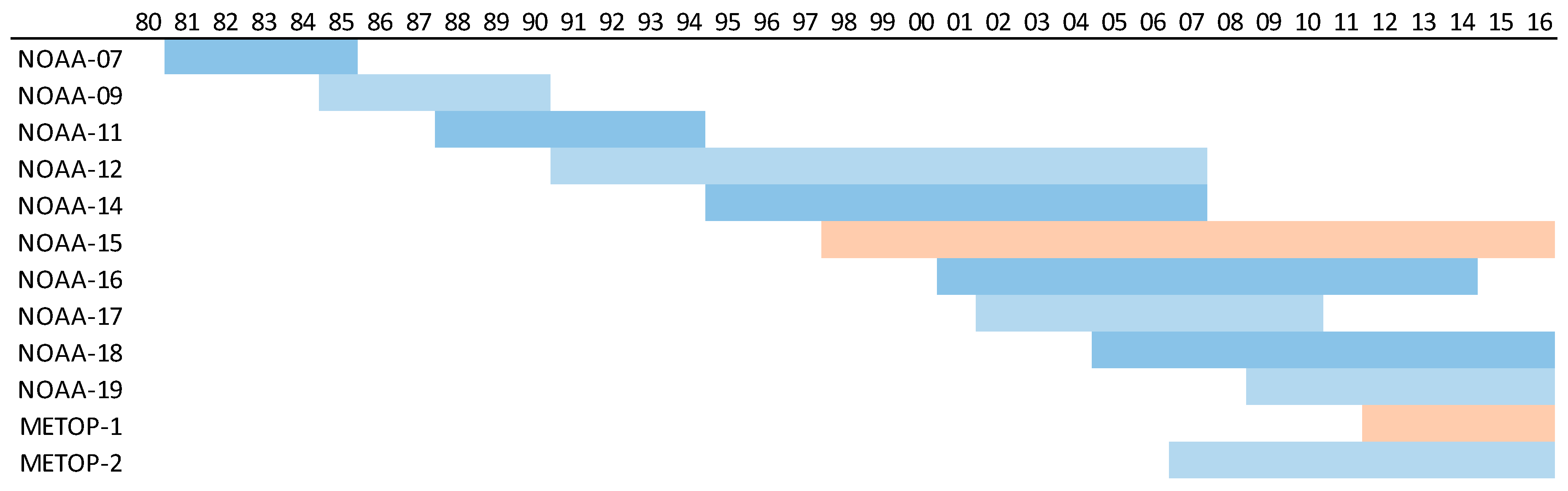
Remotesensing 10 00990 g001
Figure 2. Availability of AVHRR data by platform and by years. In blue, the data that was used for the present study, and, in red, the data that was not processed due to the elevated amount of inconsistent data.
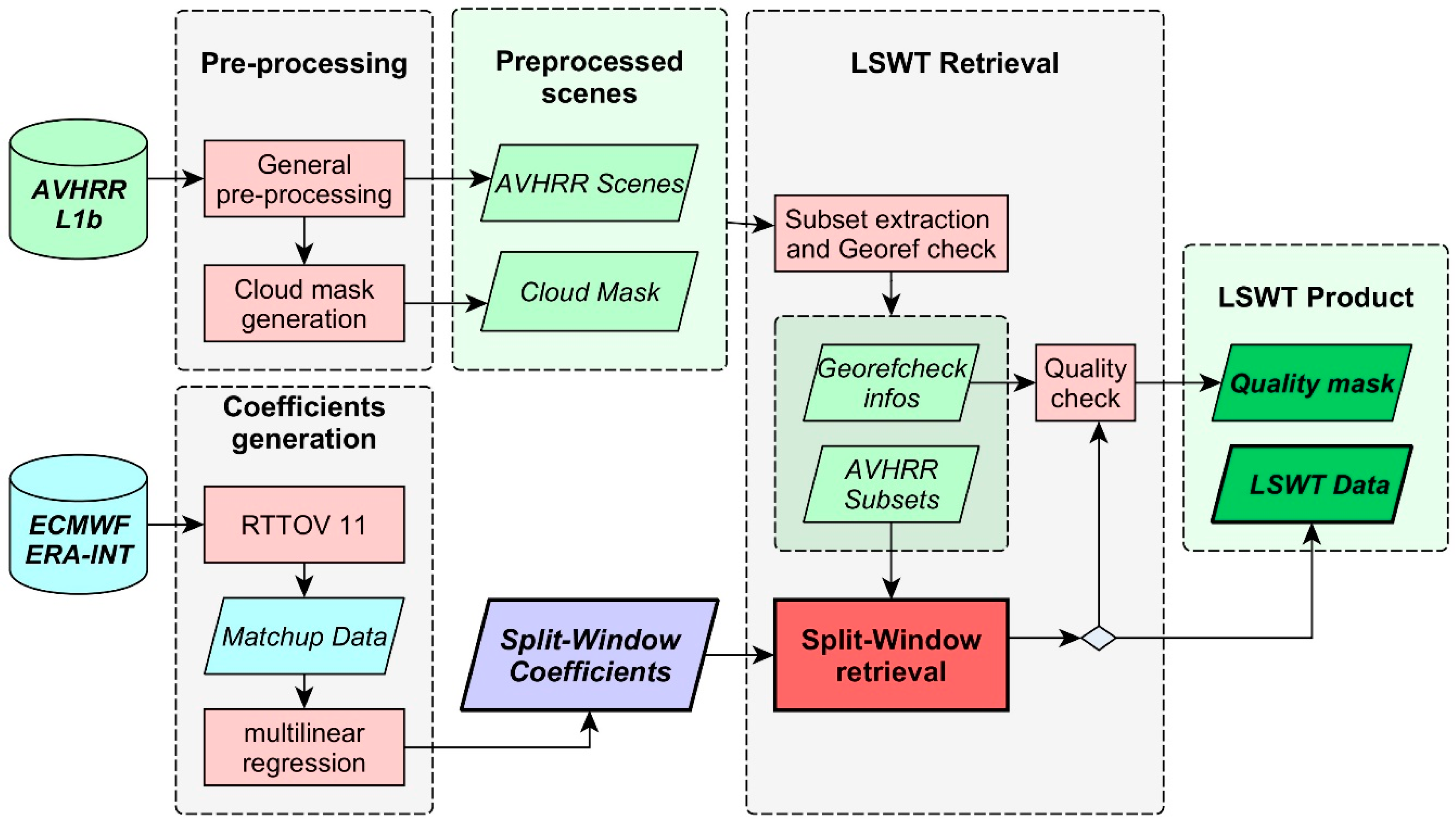
Remotesensing 10 00990 g002
Figure 3. Schematic representation of the LSWT processing as used for this work.
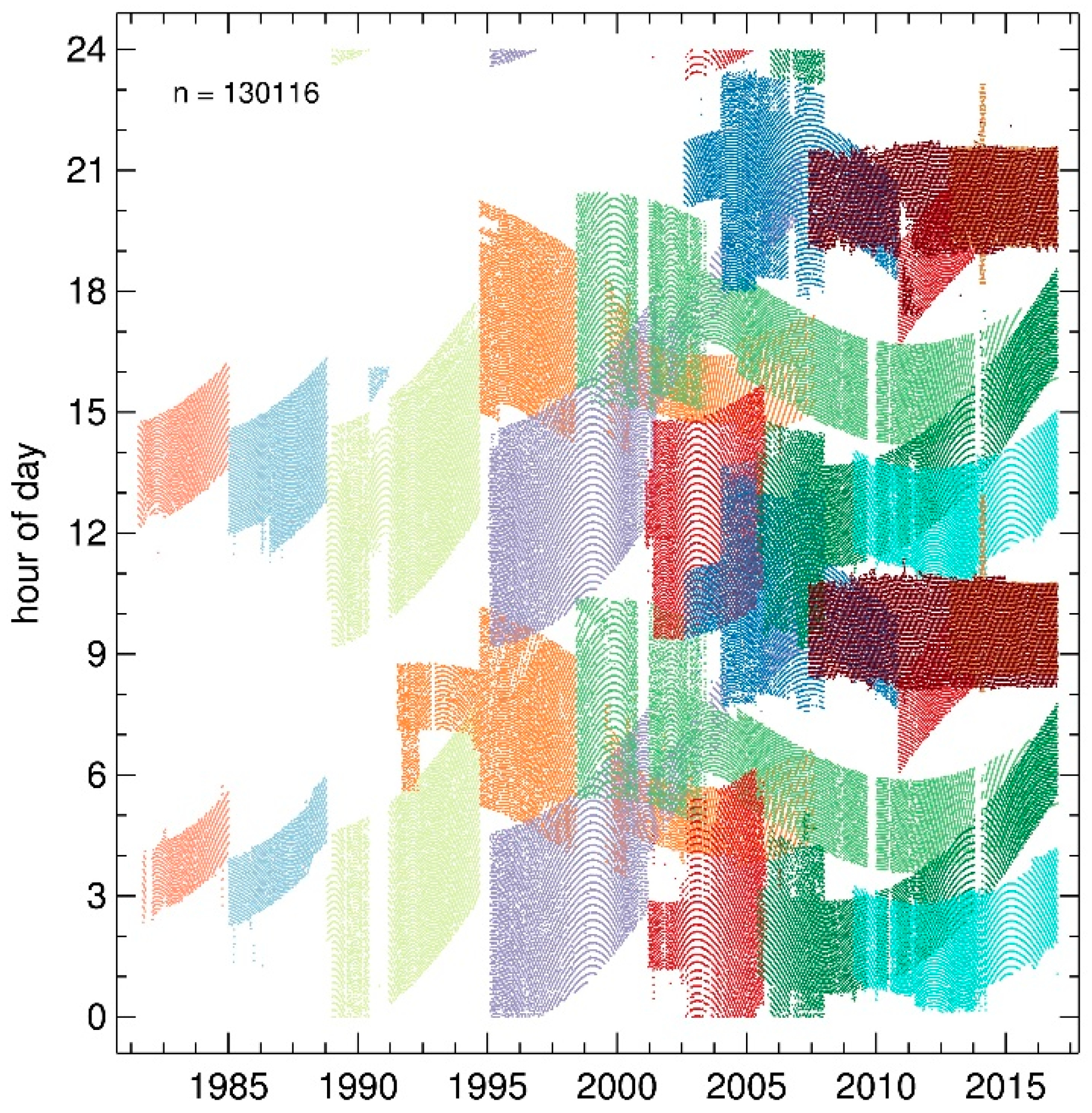
Remotesensing 10 00990 g003
Figure 4. Overpass times of all AVHRR scenes in which Lake Geneva is visible. Each dot represents a scene; the different colors represents different platforms.
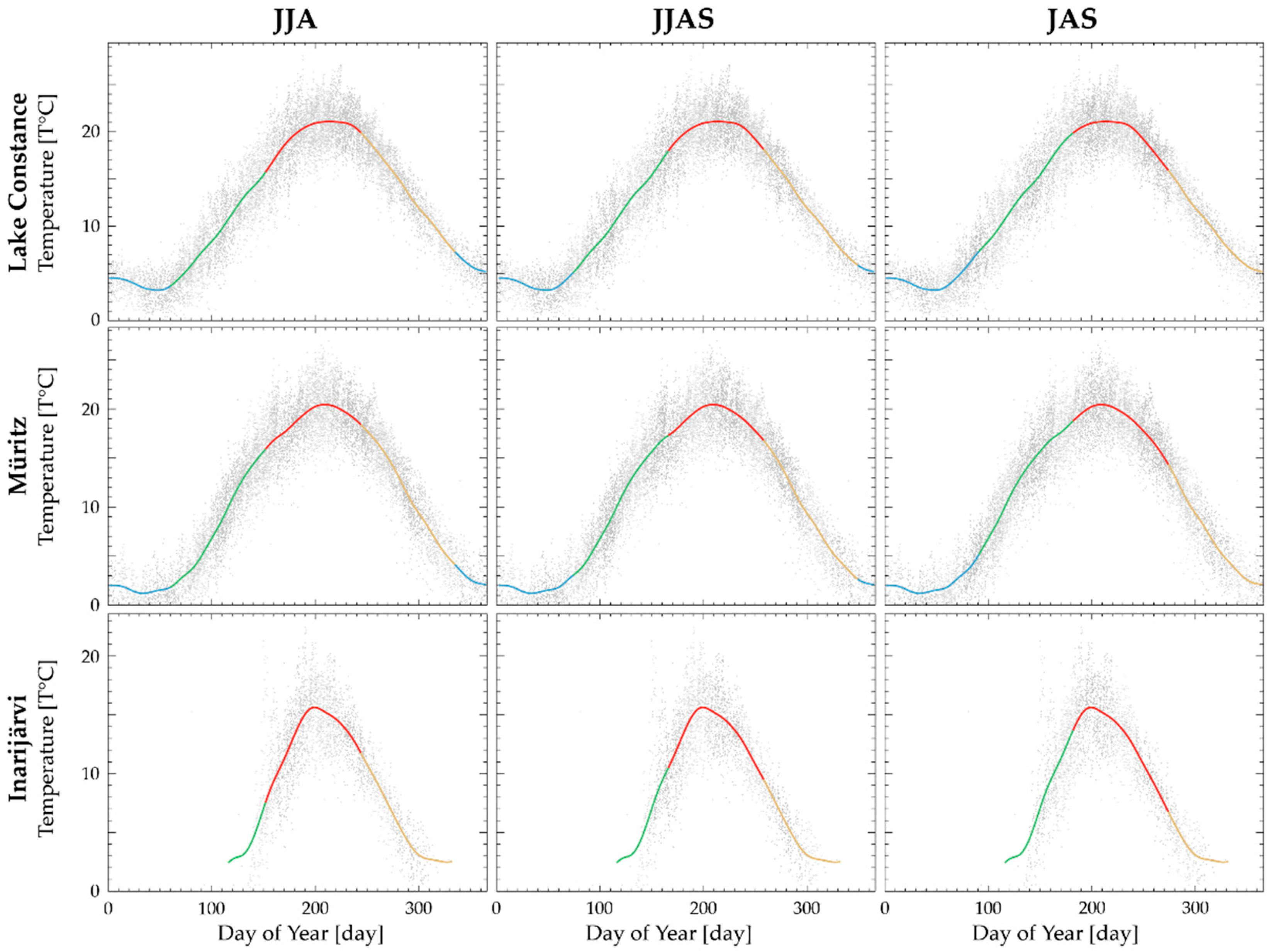
Remotesensing 10 00990 g004
Figure 5. Comparison for different season periods (JJA, JJAS, JAS) in the yearly temperature cycle at lake Constance, Müritz, and Lake Inari. The middle row, representing the seasonal periods as used during this study is well adapted to the actual annual cycles, as the summer temperature peak is in the center of the period.
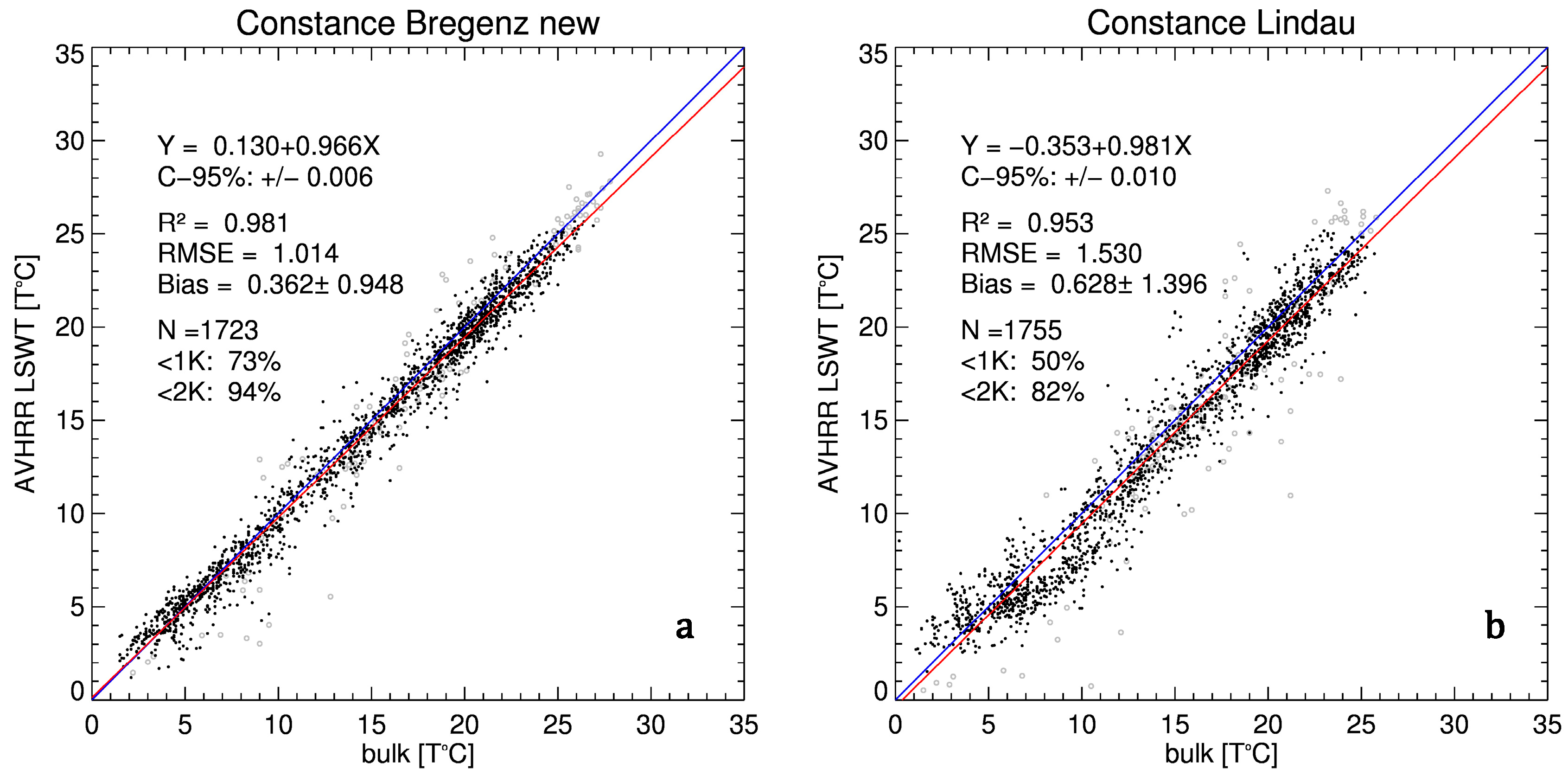
Remotesensing 10 00990 g005
Figure 6. The validation with hourly averaged measurements at Lake Constance for the station in Bregenz (a) and for the station in Lindau (b). Both show a good performance and a high number of matchups despite the in-situ locations close to the shore. However, the correlation with the satellite data is significantly higher in Bregenz (a) than in Lindau (b). For both validations, the same satellite data is used.
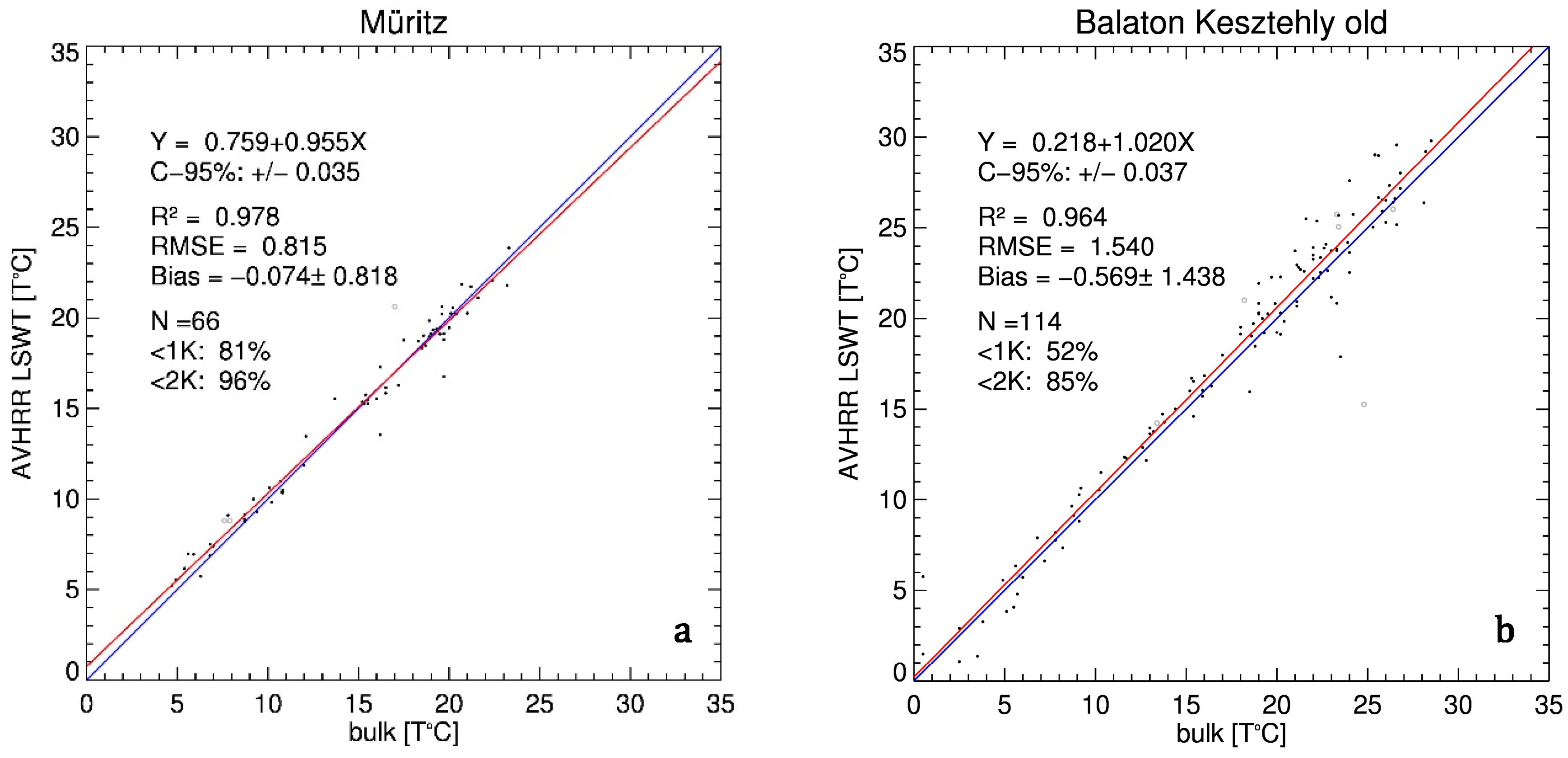
Remotesensing 10 00990 g006
Figure 7. The validation with sporadic instant measurement at Müritz (a) and at Lake Balaton (b). Both in-situ measurements where manually taken in open waters. The bi-monthly sampling frequency only allows for few matchups per year. Nevertheless, the measurements at Müritz yield the best performance thanks to close temporal matchups and the open waters. At Lake Balaton however, the exact timestamp was unknown (only day). Therefore, 12:00 local time was assumed, which led to less accurate temporal matchups and lower correlation.
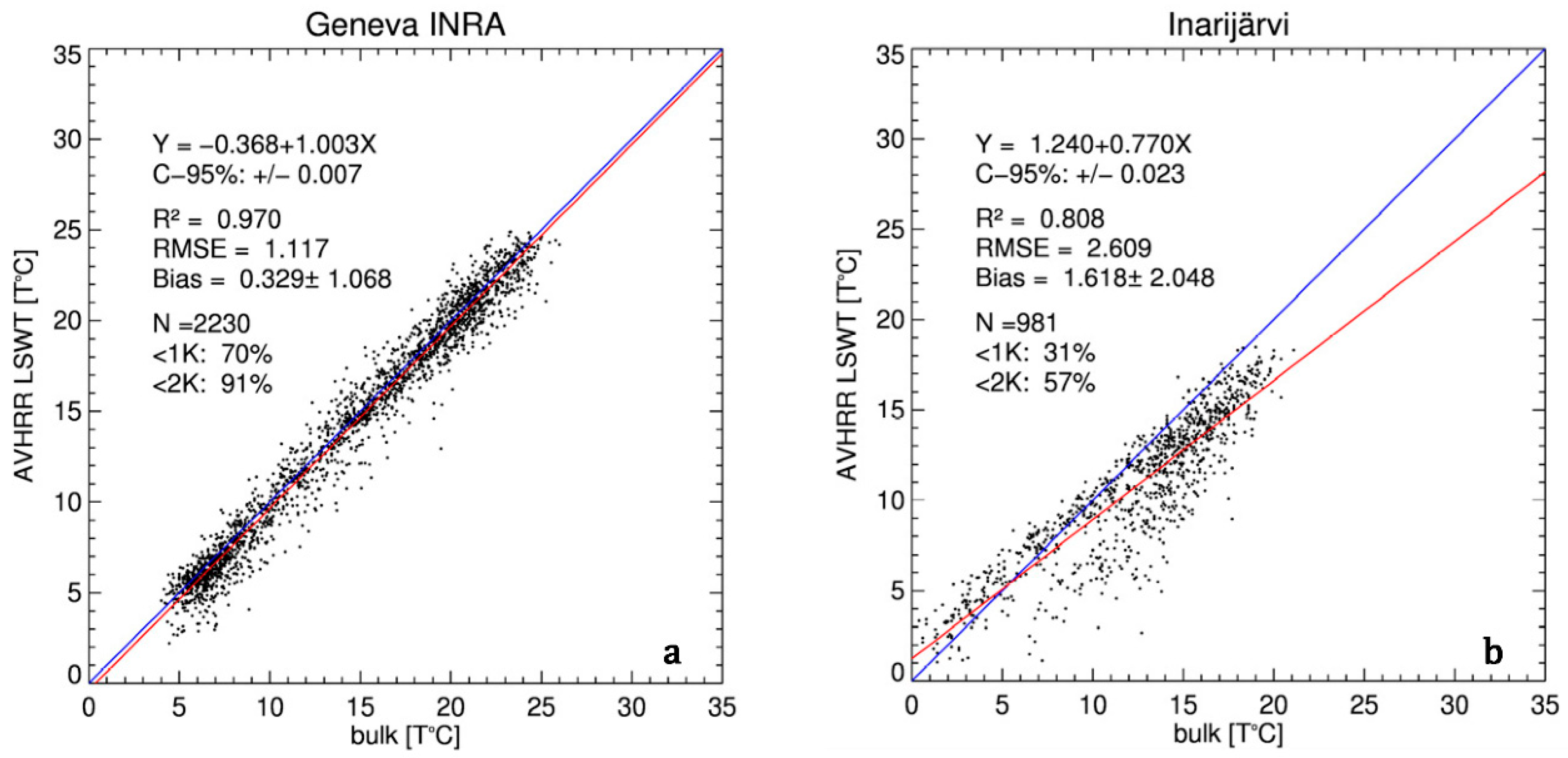
Remotesensing 10 00990 g007
Figure 8. The validation with daily in-situ measurement at Lake Geneva, INRA (a) and Inarijärvi (b). The validation at Lake Geneva INRA shows good performance and a high number of matchups through the whole year. At Inarijärvi, however, the weakest validation performance of all is found. Inarijärvi is located north of the polar cycle and has a long period of ice cover per year. Further, the in-situ measurement station is located within a very complex shore geometry with many small islands.
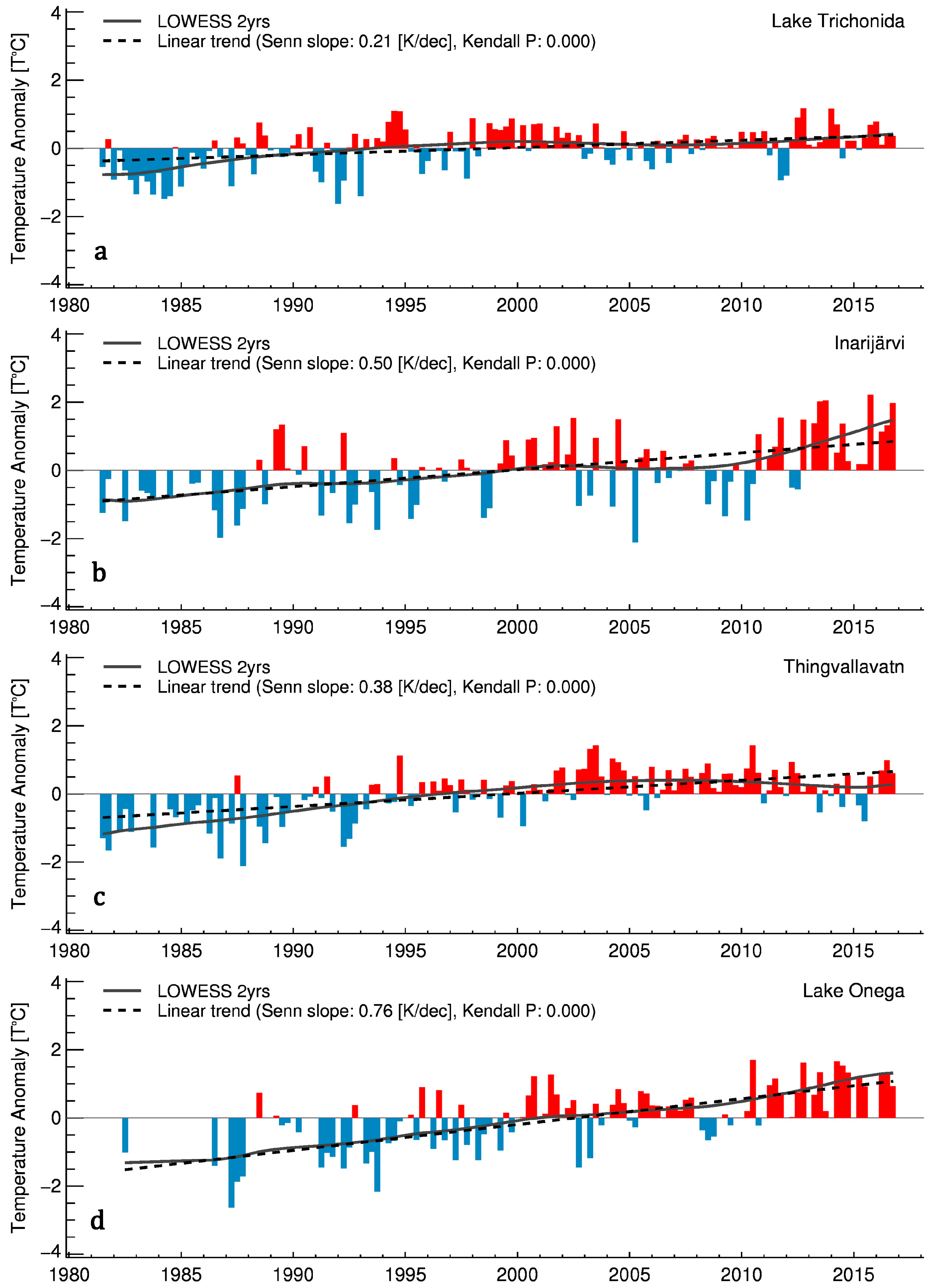
Remotesensing 10 00990 g008
Figure 9. Temperature trends of Lake Trichonidas (a), Inarijärvi (b), Thingvallavatn (c), and Lake Onega (d). Blue bars indicate temperatures below the long-term mean, whereas the red bars show warmer years. The dashed line shows the linear trend, whereas the solid black line shows the locally weighted scatterplot smoothing (LOWESS) over a 2-years period. Lake Trichonidas (a) is the lake with the lowest latitude (except for Djorf Torba), whereas Inarivjärvi (b) is the lake at highest latitude. The same applies for the longitude where it goes from Thingvallavatn (c) in the west to Lake Onega (d) in the east.
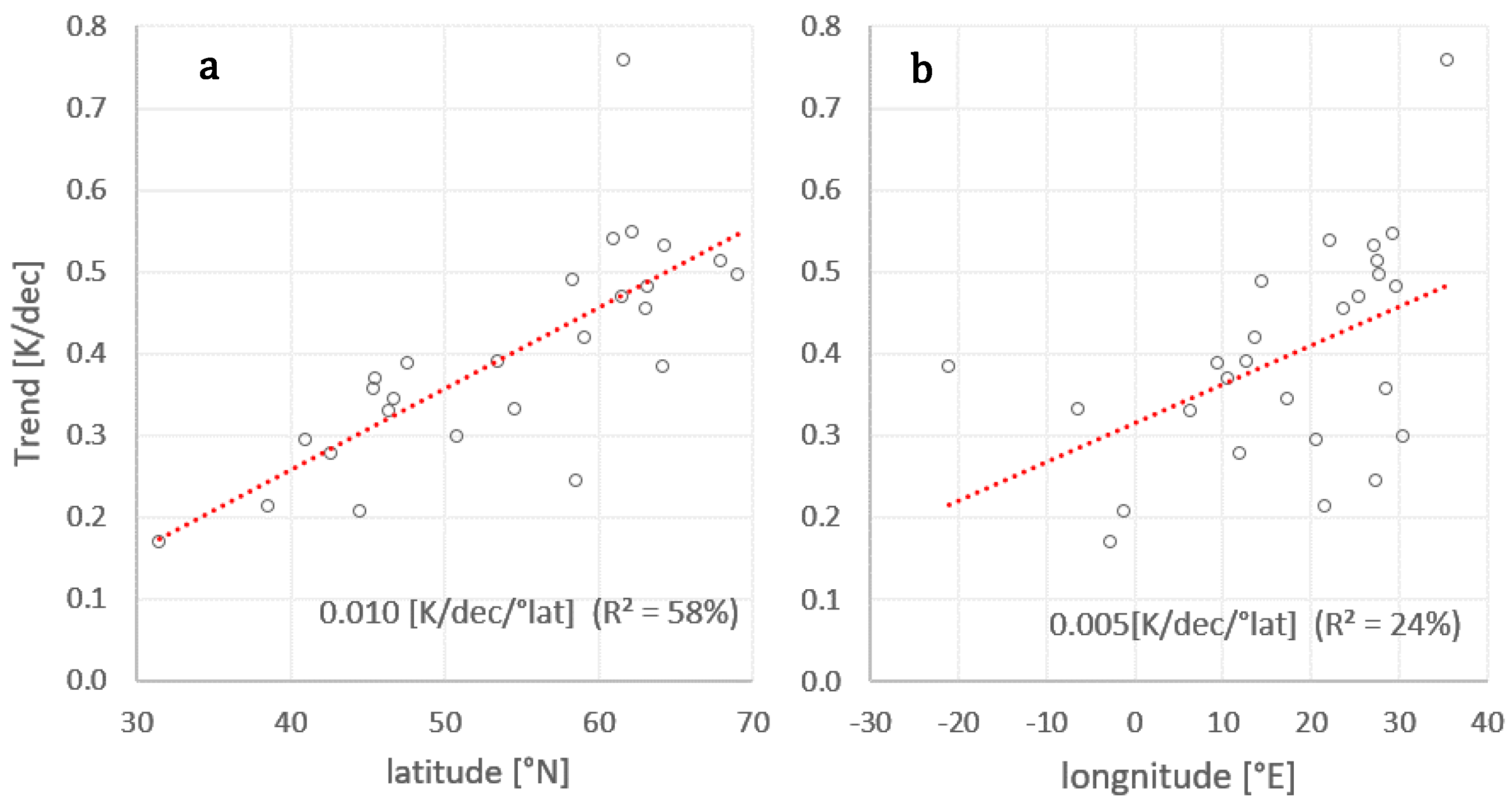
Remotesensing 10 00990 g009
Figure 10. South–north gradient (a) and the west–east gradient (b) of the yearly LSWT trend. The red dashed line is a simple linear model derived with least square regression, and R2 is the coefficient of determination.
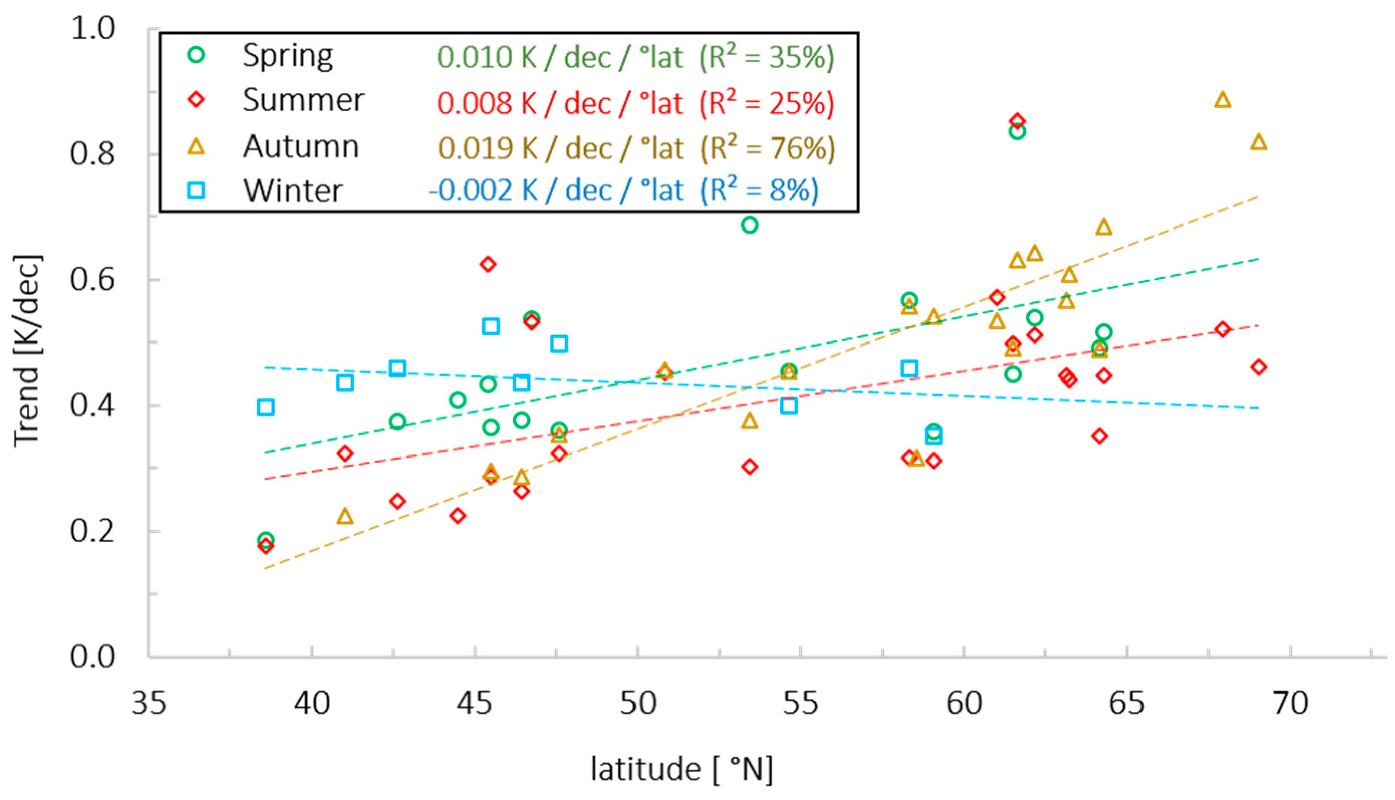
Remotesensing 10 00990 g010
Figure 11. South–North gradient of seasonal trends from European lakes. The dashed lines are simple linear models derived with least square regression of the data points. The reservoirs lakes are excluded from the graph.
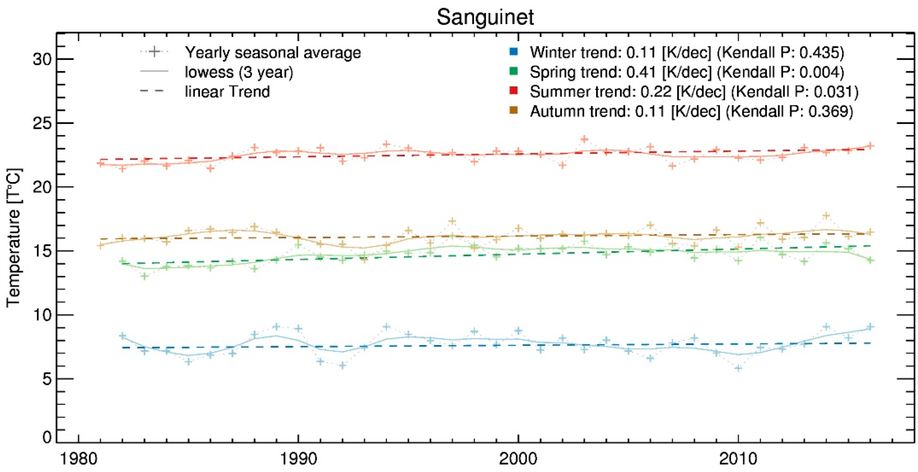
Remotesensing 10 00990 g011
Figure 12. Seasonal trends at Lake Sanguinet, whereas the spring and summer trend are categorized as ‘significant’ (p-value < 0.05); the winter and autumn trends 0.11 K/decade are categorized ‘insignificant’ (p-values > 0.05).
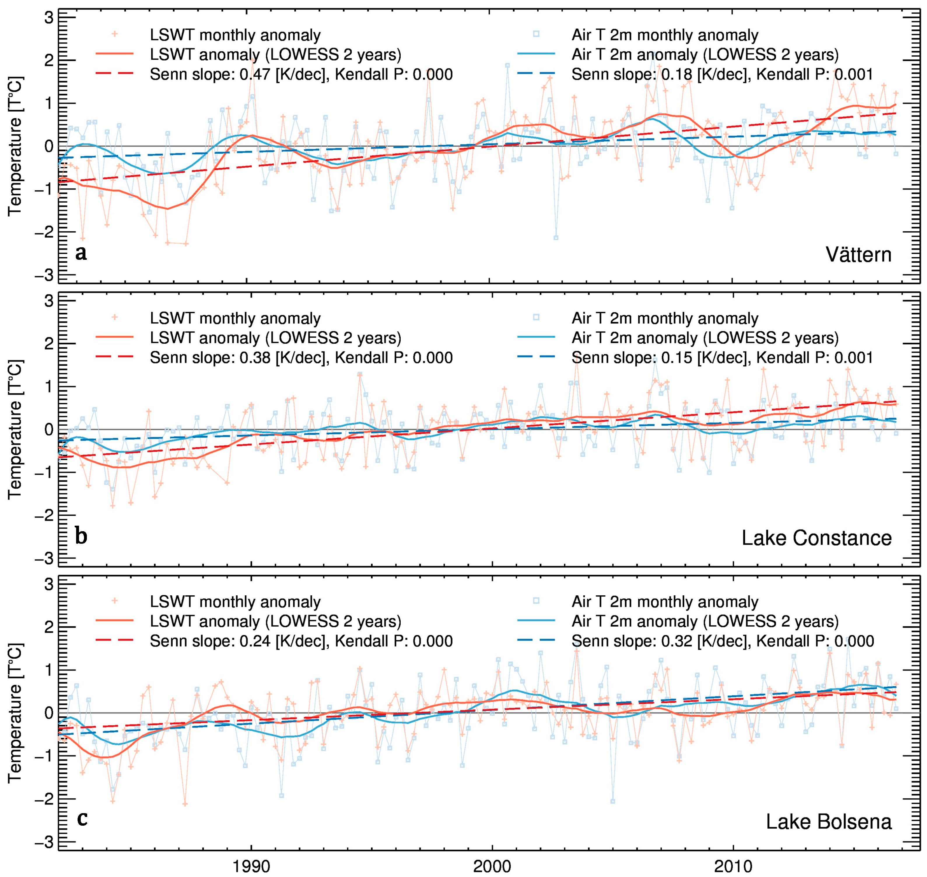
Remotesensing 10 00990 g012
Figure 13. Comparison of LSWT trends with local air temperature trends (extracted from ERA INTERIM) at Lake Vättern (a), Lake Constance (b), and Lake Bolsena (c).
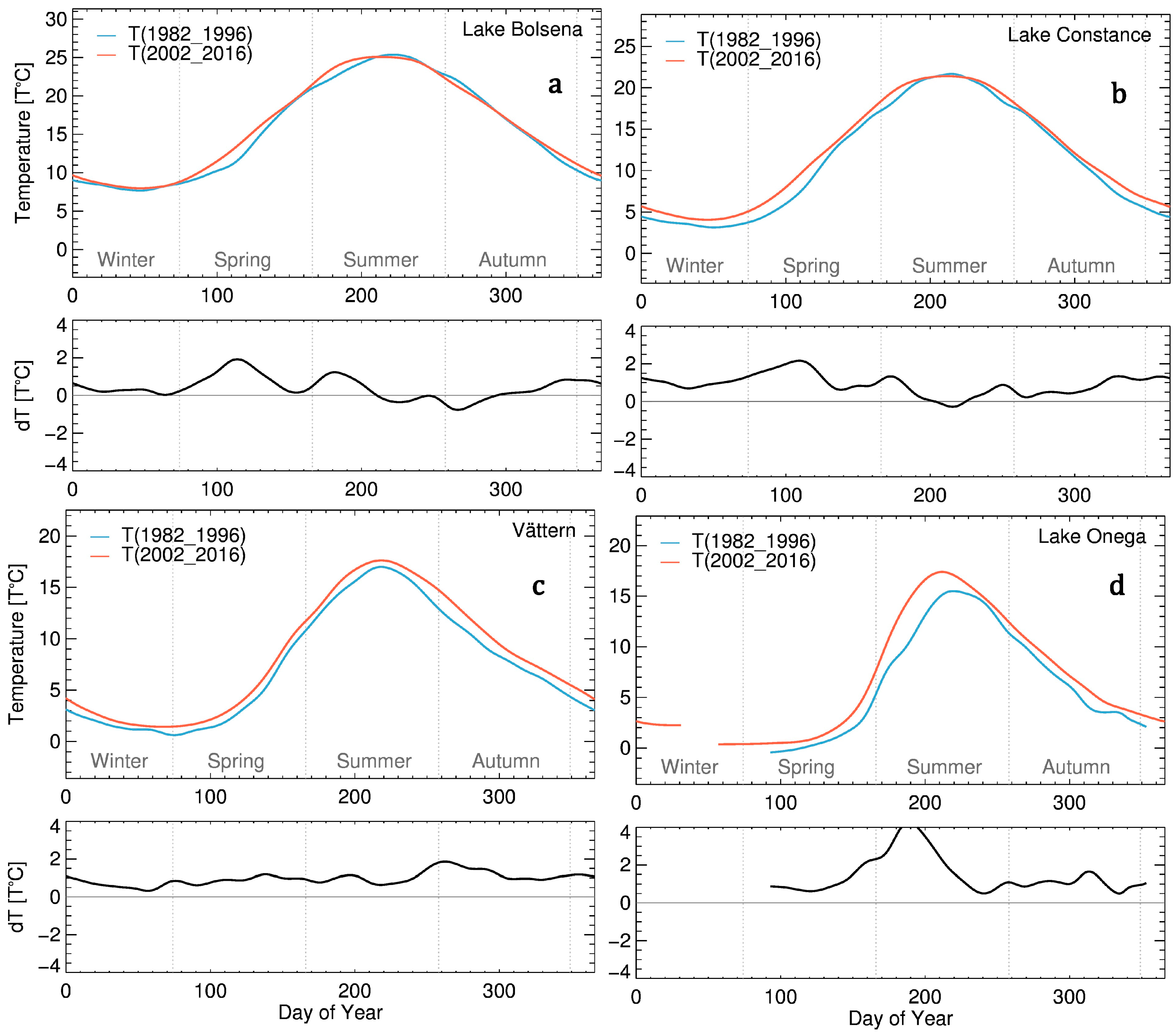
Remotesensing 10 00990 g013
Figure 14. Comparison of the Yearly Temperature Cycle from two different 15-years-periods at Lake Bolsena (a), Lake Constance (b), Lake Vättern (c), and Lake Onega (d). The red and the blue lines represent the yearly cycle of the two periods; the black line is the difference between the two periods.
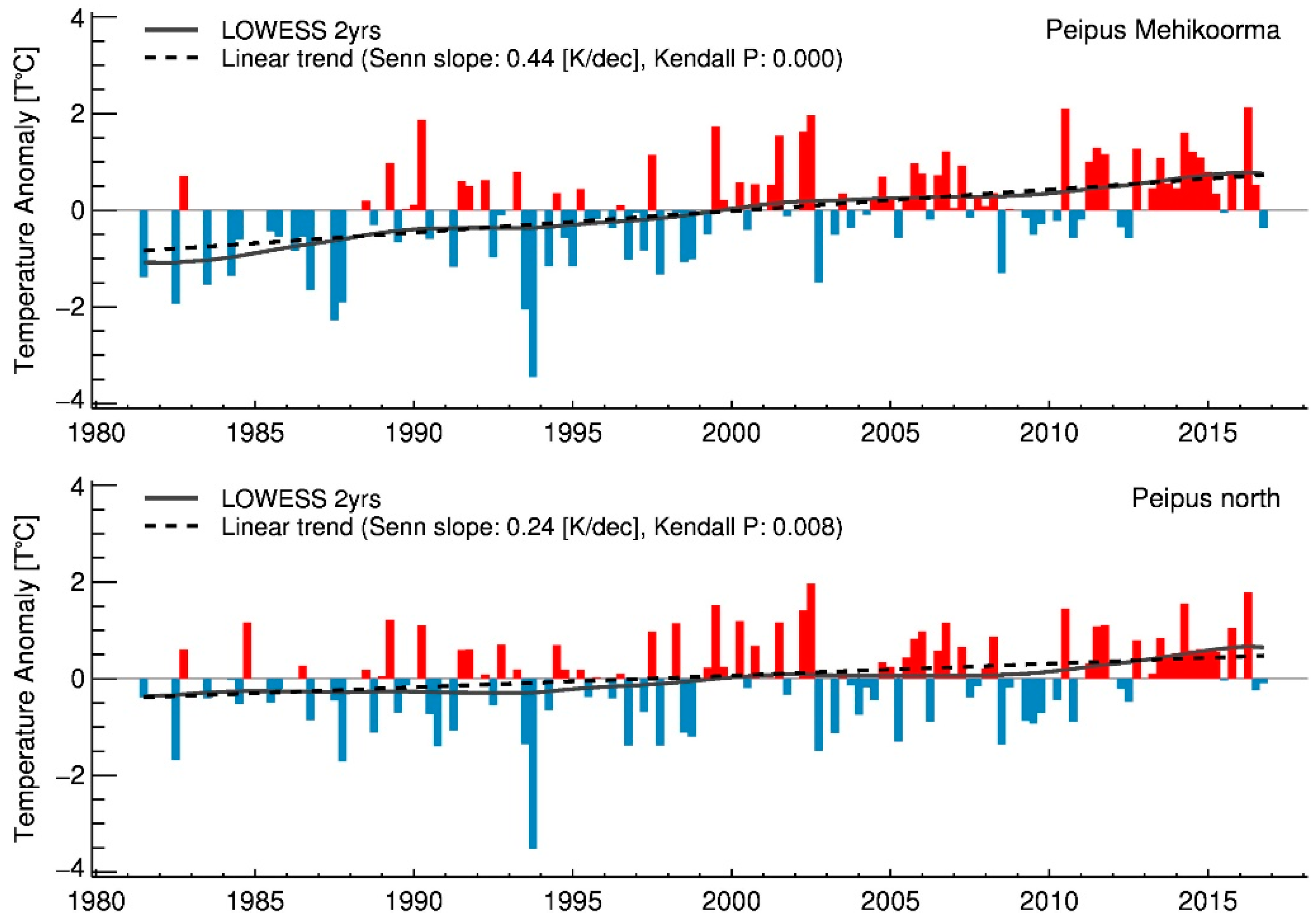
Remotesensing 10 00990 g014
Figure 15. Significant difference in trends within Lake Peipus when comparing the trend near the Mehikoorma in-situ station (see coordinates in Table 2) with the trend in the open waters of the northern part (see coordinates in Table 1).
Remotesensing 10 00990 g015
Table 1. List of Lakes where LSWT was retrieved and trend analysis performed. The acronyms are the same as those used in Figure 1.
Lake NameCountryAcr.LocationAlt. [m]Area [km2]Depth Ø [m]In-Situ Data
Lake BalatonHUBala46.75°N17.43°E1265783.3Yes
Lake BolsenaITBols42.61°N11.93°E36811481.0No
Lake ConstanceDE,CH,AUTCons47.60°N9.45°E431472101.0Yes
Djorf TorbaDZADjor31.53°N2.75°W716776.1No
Lake GardaITGard45.52°N10.67°E85368133.0No
Lake GenevaFR, CHGene46.41°N6.41°E466580152.7Yes
InarijärviFINInar69.04°N27.76°E1261′11014.0Yes
Kiev ReservoirUAKiye50.80°N30.47°E934204.0No
LappajärviFINLapp63.13°N23.71°E851417.0Yes
Lokka ReservoirFINLoka67.94°N27.56°E2594885.0No
MüritzDEMuri53.43°N12.67°E631106.5Yes
Lough NeaghNIRNeag54.62°N6.41°W583809.0No
Lake OhridMK,ALBOhri41.02°N20.72°E700347155.0No
Lake OnegaRUOneg61.63°N35.53°E569′60830.0No
OulujärviFINOulu64.29°N27.22°E1288907.6Yes
Lake PäijiänneFINPaij61.52°N25.42°E951′08016.0Yes
Lake PeipusEST,RUPeip58.53°N27.50°E293′5537.1Yes
Lake PielinenFINPiel63.24°N29.64°E1138709.0Yes
Säkylän PyhäjärviFINPyhj61.00°N22.28°E521505.5Yes
PyhäselkäFINOriv62.60°N29.77°E763618.7Yes
SanguinetFRSang44.49°N1.15°W24575.0No
ThingvallavatnISThin64.16°N21.13°W1058334.0No
Lake TrichonidaGRTric38.57°N21.57°E409530.0Yes
Lake VänernSWEVane59.07°N13.60°E455′65027.0No
Lake VätternSWEVatt58.33°N14.50°E911′89040.0No
Lake YalpuhUAYalp45.42°N28.63°E102252.0No
Table 2. List of in-situ measuring locations from which data was available for this study. Most of the measurements are either hourly or daily averaged temperatures from automatic stations. In the case of Müritz, Lake Trichonida, and the older measurements from Lake Balaton, the measurements are sporadically and manually taken at specific locations on the lake. The average measurement density varies from 12 measurements per year at Lake Trichonida (monthly measurements) to 8760 measurements per year at Bregenz, Lake Constance (hourly measurements).
LakeCountrySta. NameType/Freq.CoverageN/YrLocation
Lake BalatonHUKeszthely oldinstant1981–20032146.74°N 17.29°E
Keszthelyhourly2003–20134′04346.76°N 17.27°E
Siofokdaily1992–201236546.90°N 18.05°E
Lake ConstanceDE, CH AUTBregenz olddaily1989–199636547.51°N 9.74°E
Bregenz newhourly1997–20098′76047.51°N 9.74°E
Lindauhourly2005–20148′26147.54°N 9.68°E
Lake GenevaFR, CHBuchillonhourly2000–20118′14746.46°N 6.40°E
INRAdaily1991–201136046.38°N 6.47°E
Lake InariFINInaridaily1980–201415368.90°N 28.10°E
LappajärviFINHalkosaaridaily1980–201416763.26°N 23.63°E
MüritzDEMüritzinstant1980–20131853.42°N 12.70°E
PyhäjärviFINSäkyländaily1996–201420561.11°N 22.17°E
OulujärviFINOulujärvidaily1980–201415664.40°N 27.17°E
Lake PaijiänneFINPäijätsalodaily2003–201420061.47°N 25.59°E
Kalkkinendaily1980–199921461.29°N 25.57°E
Lake PeipsiEST, RUMehikoormadaily1985–201126758.24°N
Lake PielinenFINNurmesdaily1980–201416363.54°N
PyhäselkäFINJoensuudaily1980–201419462.60°N
Lake TrichonidaGRETrichonidainstant2004–20061238.57°N
Table 3. The six quality levels indicate which additional tests are passed. The levels are cumulative (e.g., Q4 means Q3 AND VZA < 55). The average data availability (compared to Q1) and the average standard deviation during the validation are shown for the different quality levels.
Quality LevelPerc. N (%)Stddev
Q1valid pixels *100.0%1.399
Q2SSDEV < 399.9%1.395
Q3no Sun glint95.9%1.390
Q4VZA < 5589.7%1.362
Q5VZA < 4583.7%1.344
Q6feature detection passed **66.4%1.333
* Cloud and land mask applied, and physical inconsistency removed; ** passed if the detection of the feature is confirmed (additional georeferentiation test).
Table 4. Validation results for each in-situ station. The data is ordered by latitude from south to north. The measurement type describes the averaging of the in-situ measurement: daily averaged, hourly averaged, and instant measurements. Instant measurements are single measurements that were manually taken during measurement campaigns. As the exact timestamps for the instant measurements where not known at Lake Balaton (Kesztehly old) and Lake Trichonida, 12:00 local time is assumed.
LocationTypeLocationn MatchRRMSEBIAS ± SD
Lake TrichonidaInstant *38.57°N21.56°E160.9871.59−1.23 ± 1.04
Geneva INRAdaily46.38°N6.47°E24530.9851.080.26 ± 1.05
Geneva Buchillonhourly46.46°N6.40°E23730.9811.29−0.52 ± 1.18
Balaton Kesztehly oldInstant *46.74°N17.29°E1140.9821.54−0.57 ± 1.44
Balaton Keszthely newhourly46.76°N17.27°E10500.9661.450.69 ± 1.27
Balaton Siofokdaily46.90°N18.05°E28340.9851.47−0.54 ± 1.36
Constance Bregenz newhourly47.51°N9.74°E17230.9901.010.36 ± 0.95
Constance Bregenz olddaily47.51°N9.74°E7190.9811.370.50 ± 1.28
Constance Lindauhourly47.54°N9.68°E17550.9761.530.63 ± 1.40
Müritzinstant53.42°N12.70°E660.9890.82−0.07 ± 0.82
Peipsi Mehikoormadaily58.24°N27.48°E21020.9841.250.44 ± 1.17
Pyhäjärvi Säkylädaily61.11°N22.17°E17490.9751.260.36 ± 1.21
Päijänne Päjätsalodaily61.29°N25.57°E10170.9472.061.28 ± 1.61
Päijänne Kalkkinendaily61.47°N25.59°E7220.9641.49−0.61 ± 1.36
Pyhäselka Joensuudaily62.60°N29.77°E18930.9621.460.11 ± 1.46
Lappajärvidaily63.26°N23.63°E20440.9491.570.25 ± 1.55
Pielinendaily63.54°N29.13°E17070.9381.830.45 ± 1.77
Oulujärvidaily64.40°N27.17°E19730.9261.930.56 ± 1.84
Inarijärvidaily68.90°N28.10°E12070.8962.601.65 ± 2.01
* No exact timestamp available (day only). 12 a.m. local time is assumed.
Table 5. Impact of the DTC correction on the validation with daily in-situ data. Whereas for Lake Balaton Siofok, the improvement is neglectable, a considerable performance improvement is observed, for example, at Lake Constance, Bregenz old.
LocationBIAS ± SDSD Change
Raw LSWTDTC Corr.
Balaton Siofok−1.05 ± 1.37−0.54 ± 1.36−0.1%
Päijänne Päjätsalo1.11 ± 1.631.28 ± 1.61−1.4%
Peipsi Mehikoorma0.01 ± 1.220.44 ± 1.17−3.5%
Pyhäjärvi Säkylä0.12 ± 1.260.36 ± 1.21−4.2%
Pyhäselka Joensuu−0.07 ± 1.520.11 ± 1.46−4.3%
Päijänne Kalkkinen−0.75 ± 1.42−0.61 ± 1.36−4.7%
Pielinen0.31 ± 1.870.45 ± 1.77−5.1%
Geneva INRA−0.09 ± 1.110.26 ± 1.05−5.5%
Lappajärvi0.13 ± 1.670.25 ± 1.55−7.5%
Oulujärvi0.52 ± 2.000.56 ± 1.84−7.9%
Inarijärvi1.59 ± 2.371.65 ± 2.01−15.5%
Constance, Bregenz old−0.01 ± 1.510.50 ± 1.28−15.6%
Table 6. Comparison of trends from satellite-derived LSWT with trends from in-situ data records. Only in-situ stations with data covering at least 25 years were used. The difference between DTC-adjusted trends and in-situ trends, as well as the difference between raw LSWT trends and in-situ trends, is shown in the last two columns.
LocationsYrIn-Situ TrendDTC TrendRAW TrendDiff. with In-Situ
sennpsennpsennpDTCRAW
Inarijärvi310.420.0000.450.0000.580.0000.030.16
Pyhäselka Joensuu320.580.0000.590.0000.560.0000.000.02
Peipsi Mehikoorma260.440.0000.440.0030.450.0040.000.01
Lappajärvi310.450.0000.500.0000.221.0000.050.23
Pielinen310.500.0000.640.0000.530.0000.140.03
Oulujärvi310.430.0000.490.0000.590.0000.060.15
0.050.10
Table 7. Yearly and seasonal trends at all studied locations ordered from South to North. The covered period is slightly below the maximum of 36 years, depending on availability of cloud-free scenes at each location. The grayed-out values are trends (K/dec) in which Kendall p-value > 0.They are not retained to compute the average trends showed on the last line. The strongest seasonal trend of each lake is marked with an asterisk. Blank values signify that there were not enough values to compute trends, mostly due to ice cover during the cold period.
LocationPeriodYearlyWinterSpringSummerAutumn
Yrssennpsennpsennpsennpsennp
Djorf Torba34.90.170.03−0.080.720.070.670.47 *0.000.200.23
Lake Trichonida35.50.210.000.40 *0.000.180.020.180.000.160.16
Lake Ohrid35.50.290.000.44 *0.000.180.100.320.000.230.03
Lake Bolsena35.50.280.000.46 *0.000.370.000.250.020.090.25
Sanguinet35.40.210.000.110.430.41 *0.000.220.030.110.37
Lake Yalpuh35.40.360.000.150.550.430.050.63 *0.000.230.09
Lake Garda35.40.370.000.53 *0.000.370.000.290.000.300.01
Lake Geneva35.50.330.000.44 *0.000.380.010.260.020.290.03
Lake Balaton35.40.340.000.170.570.54 *0.000.530.000.120.29
Lake Constance35.50.390.000.50 *0.000.360.000.320.000.350.00
Kiev Reservoir35.40.300.000.010.660.240.210.450.000.46 *0.03
Müritz35.40.390.000.100.550.69 *0.000.300.040.380.02
Lough Neagh35.40.330.000.400.020.450.000.040.830.46 *0.00
Vättern35.50.490.000.460.000.57 *0.000.320.010.560.00
Lake Peipus35.30.240.010.540.100.130.530.250.080.32 *0.05
Vänern35.40.420.000.350.030.360.040.310.020.54 *0.00
Pyhäjärvi35.30.540.000.570.050.470.050.57 *0.000.540.00
Lake Päijiänne35.40.470.000.760.180.450.040.50 *0.000.490.00
Lake Onega35.20.760.00 0.840.000.85 *0.000.630.00
Pyhäselkä35.30.550.00 0.540.010.530.010.57 *0.00
Lappajärvi35.20.450.00 0.400.160.450.010.57 *0.00
Pielinen35.30.480.00 0.390.260.440.010.61 *0.00
Thingvallavatn35.30.380.00 0.49 *0.000.350.010.49 *0.00
Oulujärvi35.30.530.00 0.520.030.450.000.68 *0.00
Lokka Reservoir35.30.510.00 0.520.000.89 *0.00
Inarijärvi35.30.500.00 0.460.010.82 *0.00
AVG (p < 0.05) 0.40 0.44 0.47 0.41 0.51
* Season with the highest trend per lake.

