An Automated Model to Classify Barrier Island Geomorphology Using Lidar Data and Change Analysis (1998–2014)


Abstract
:
1. Introduction
2. Methods
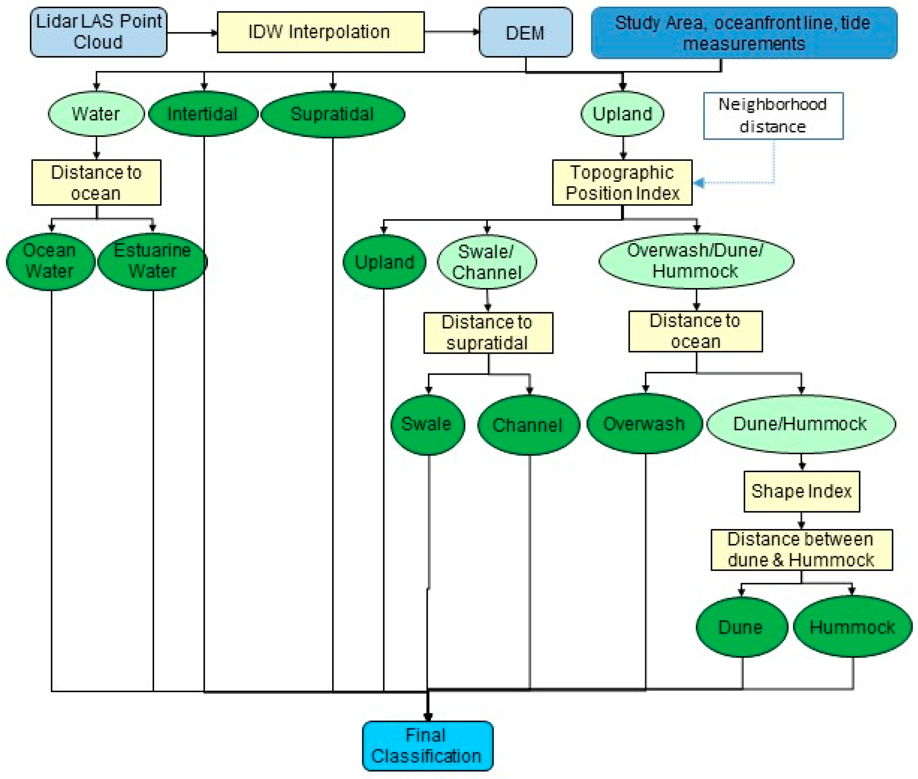
- Intertidal: Region that is inundated daily due to tides. Land above Mean Sea level (MSL) and below Mean Higher High Water (MHHW). MSL is defined as the arithmetic mean of hourly water heights of each tidal day over a 19-year period, known as the National Tidal Datum Epoch (NTDE). MHHW is defined as the average of all the higher- high water heights of each tidal day over the NTDE (see NOAA Tides and Currents, https://tidesandcurrents.noaa.gov/datum_options.html).
- Supratidal: Region that is inundated occasionally due to astronomically high tides or severe weather events. Land above MHHW and below Highest Astronomical Tide (HAT) (see NOAA Tides and Currents, https://tidesandcurrents.noaa.gov/datum_options.html).
- Dune: Linear feature that is parallel to the shoreface and has the highest elevation on the island.
- Hummock: Relic dune, usually located behind the primary dune, and is lower elevation than dunes, but higher elevation than other surrounding features (usually upland). They are usually a round shape from erosion due to wind and rain.
- Overwash: Slightly elevated and flat areas located in the back barrier and created from sediment transport from the oceanfront. Also known as overwash fans.
- Swale: Low depression located between dunes and upland areas.
- Channel: Low depression, cut by water, located adjacent to the supratidal region.
- Upland: Flat portions of the barrier island, behind the primary dune; all land that is not classified as one of the other features listed above.
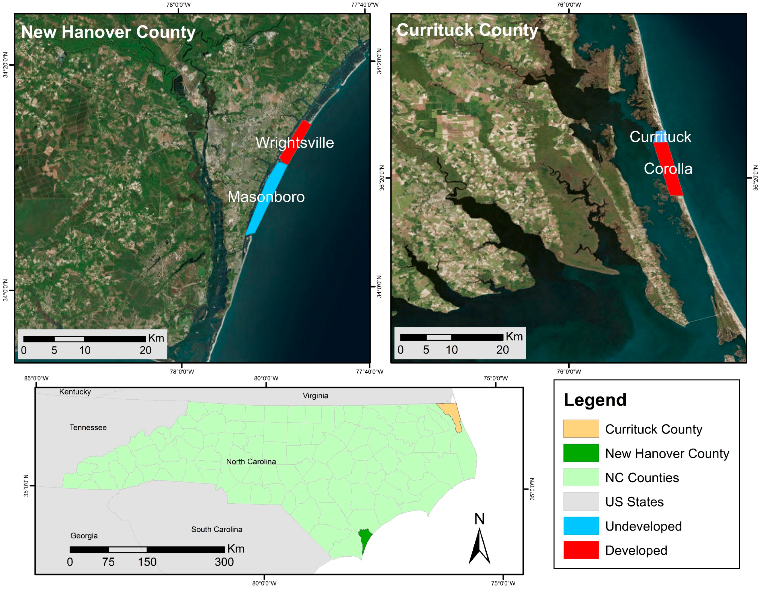
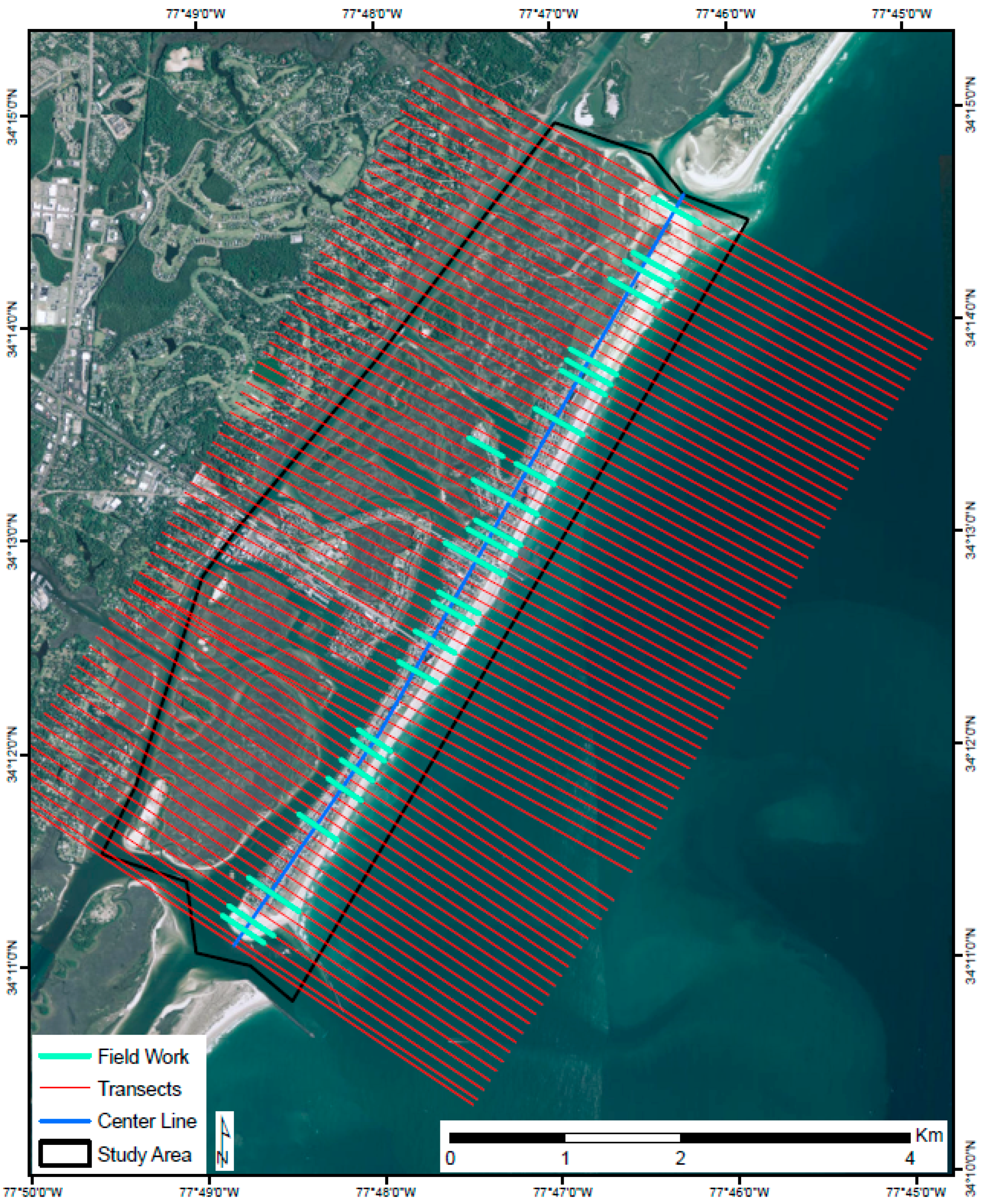
2.1. Fieldwork
2.2. Lidar Data
2.3. Geomorphic Classification
2.4. Temporal Change Analysis
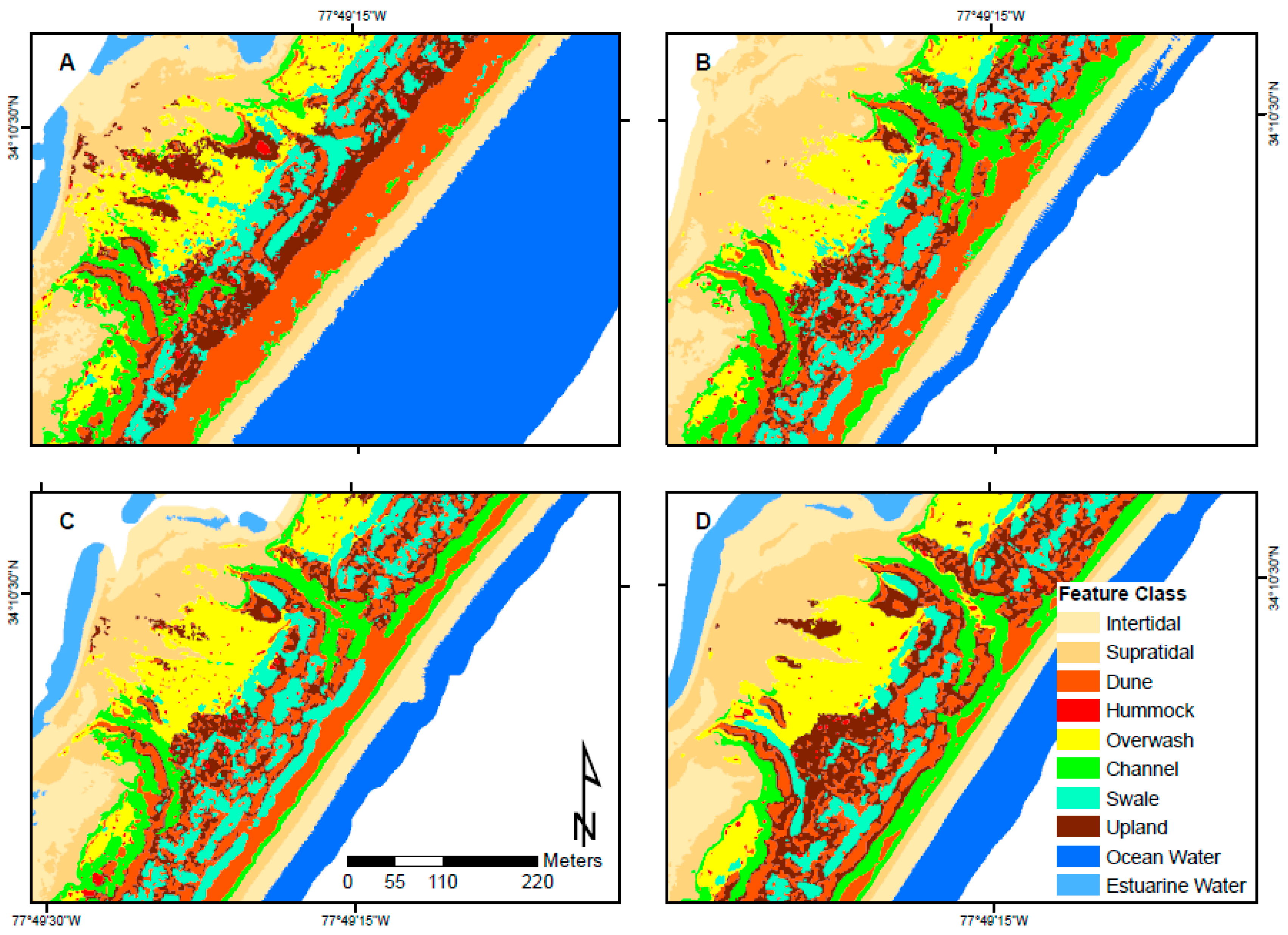
3. Results
3.1. Accuracy Assessment
3.2. Geomorphology Change through Time
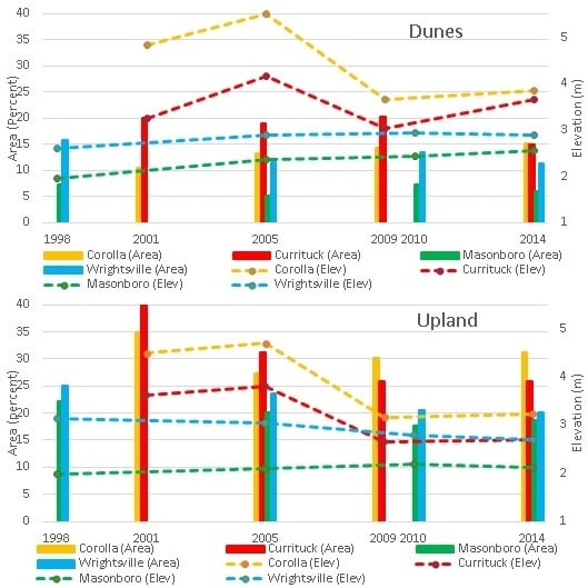
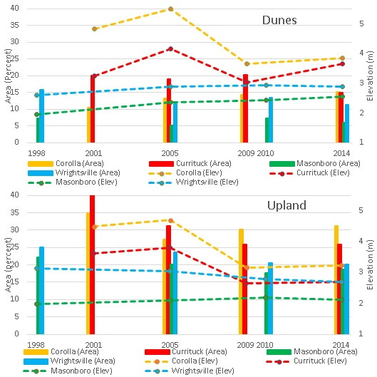
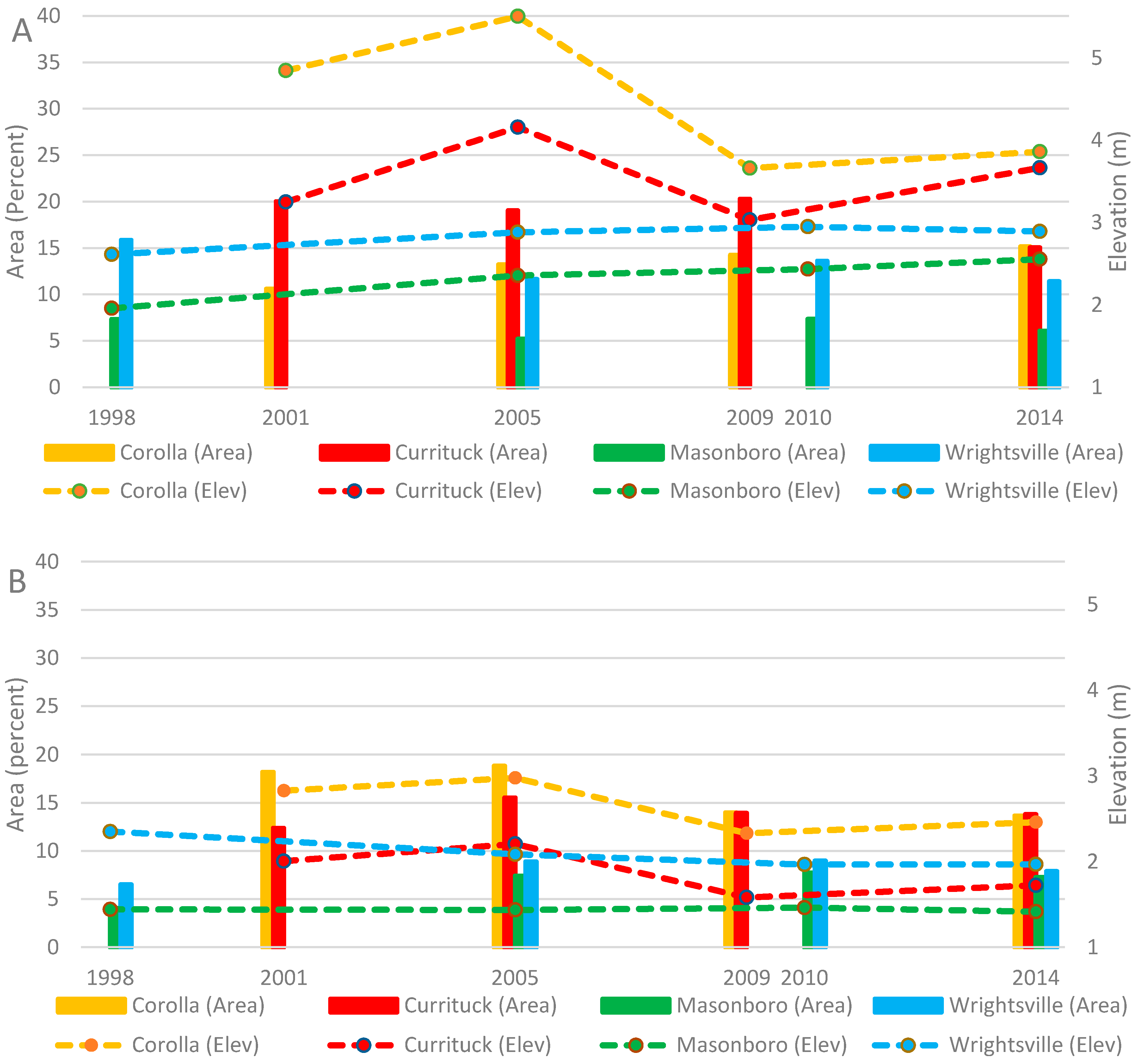
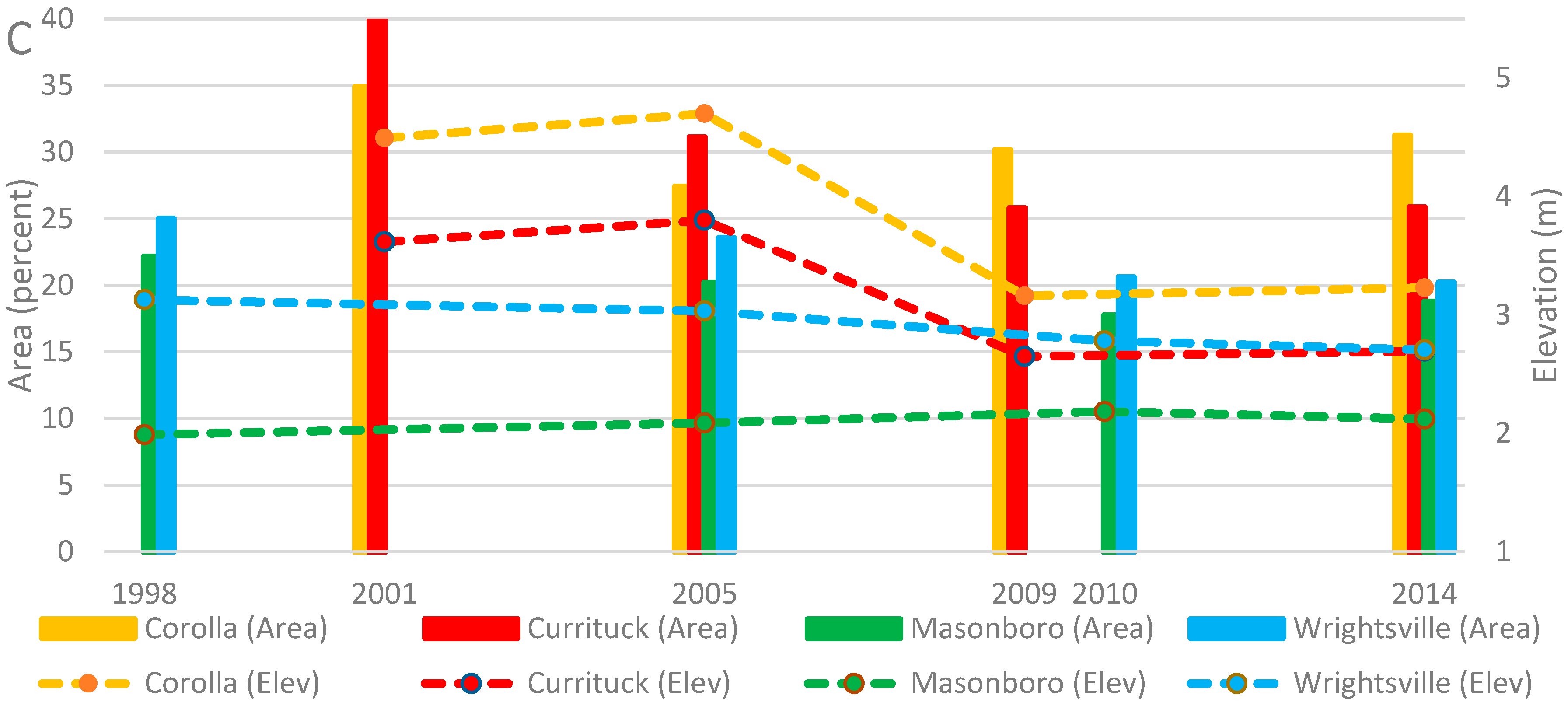
3.2.1. Change in Area and Elevation
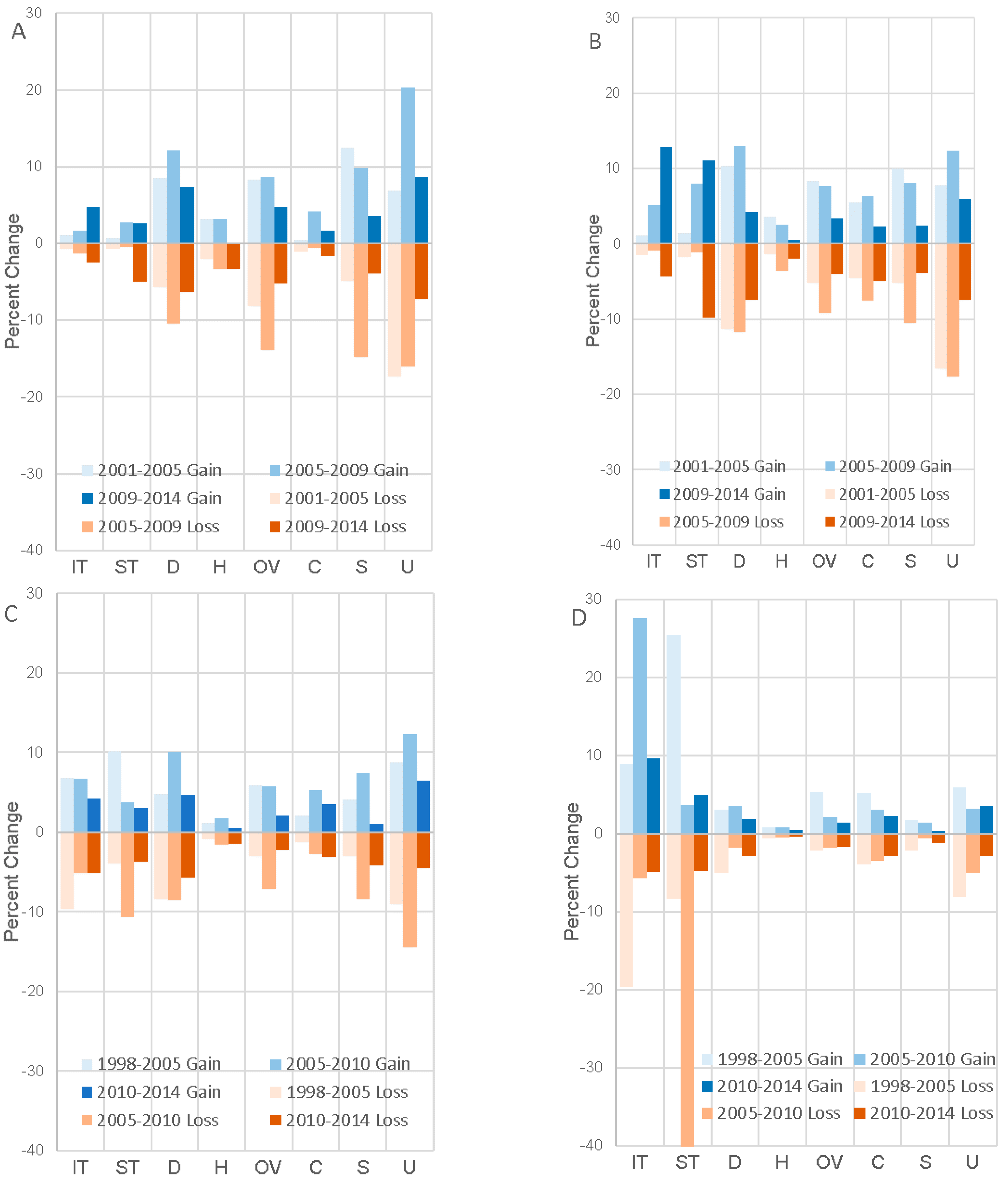
3.2.2. Geomorphology Change with Respect to Gain and Loss
3.2.3. More Change Than Expected
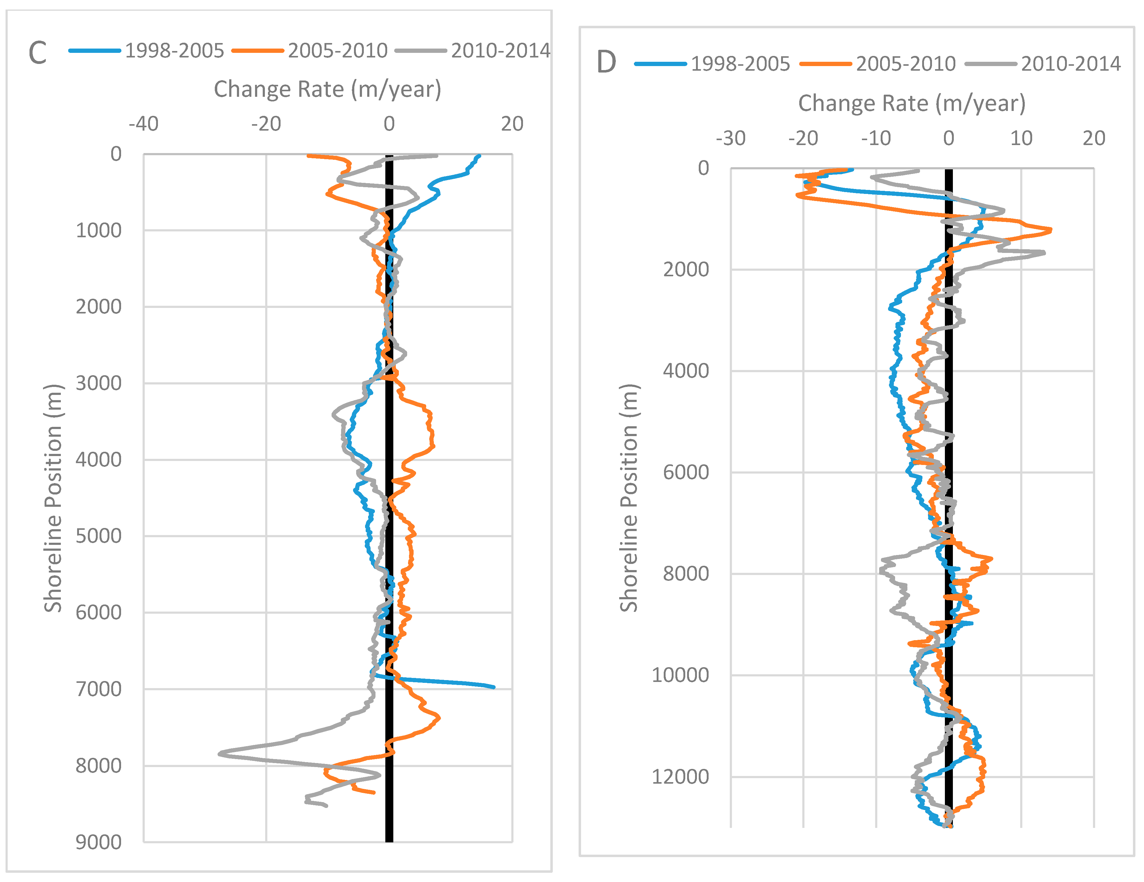
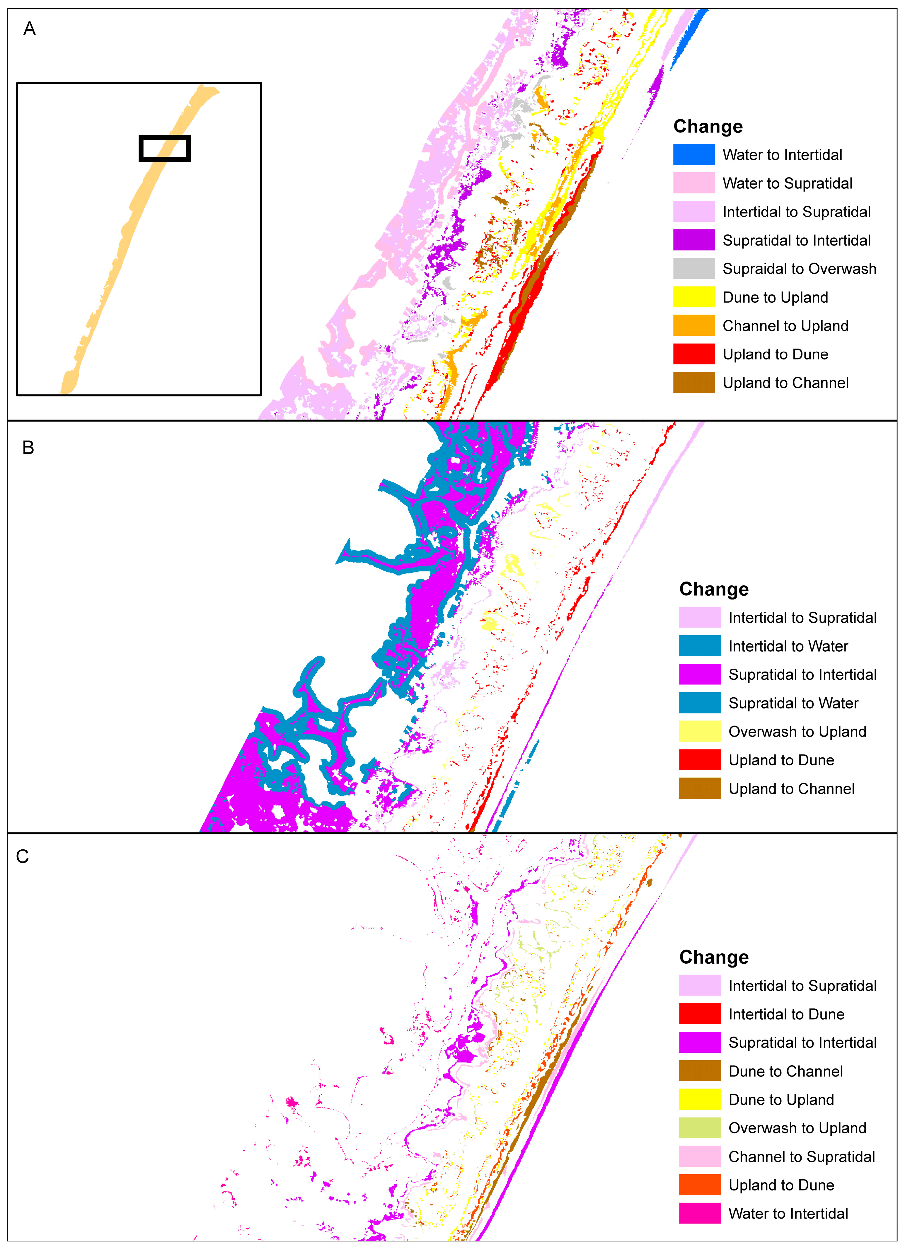
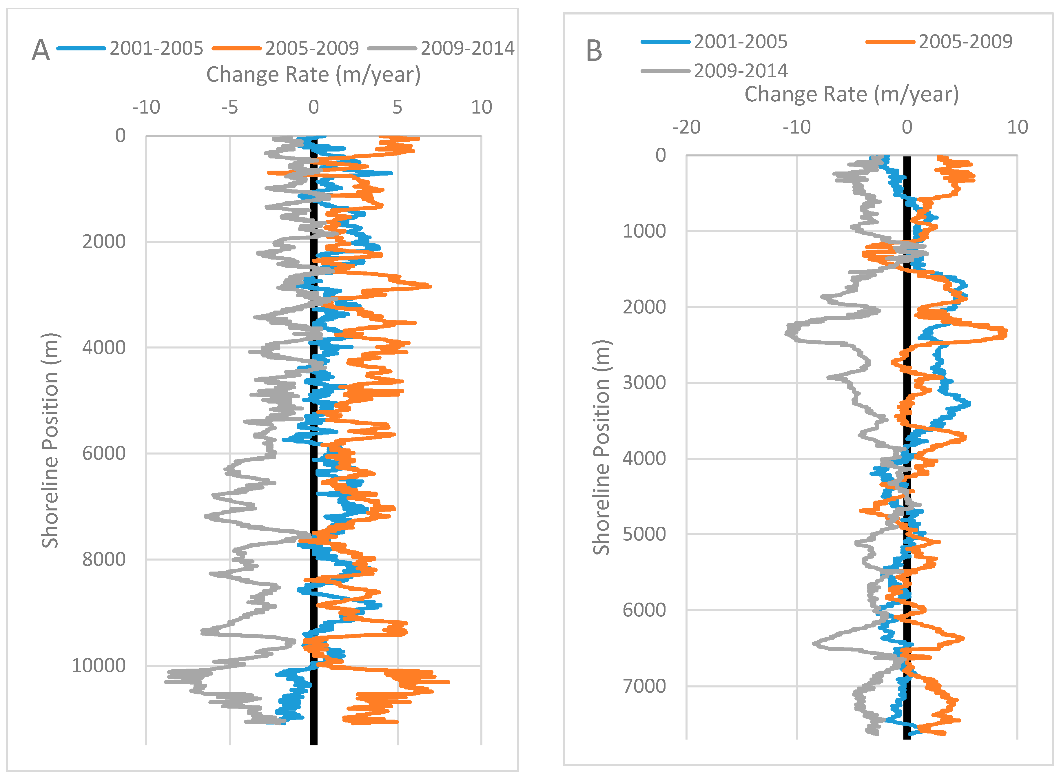
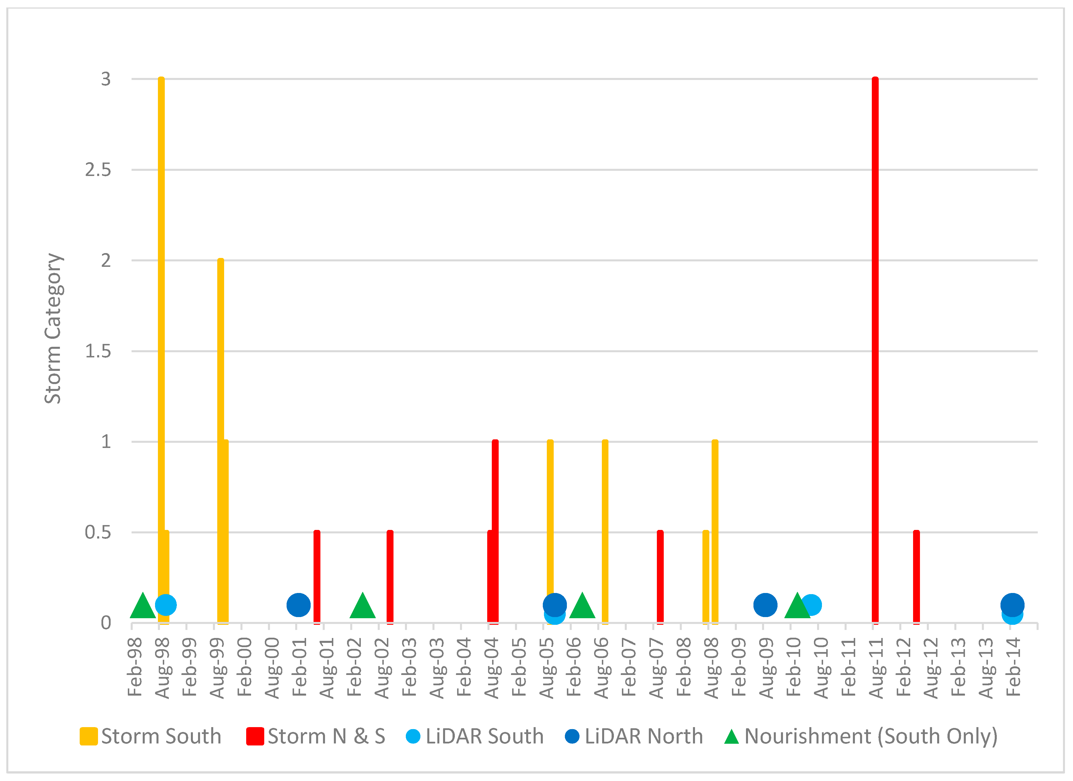
3.2.4. Shoreline Change and Dune Movement
4. Discussion
5. Conclusions
Supplementary Materials
Author Contributions
Funding
Acknowledgments
Conflicts of Interest
References
- Paris, P.; Mitasova, H. Barrier island dynamics using mass center analysis: A new way to detect and track large-scale change. ISPRS Int. J. Geo-Inf. 2014, 3, 49–65. [Google Scholar] [CrossRef]
- White, S.A.; Wang, Y. Utilizing dems derived from lidar data to analyze morphologic change in the North Carolina coastline. Remote Sens. Environ. 2003, 85, 39–47. [Google Scholar] [CrossRef]
- Dolan, R.; Hayden, B.; Lins, H. Barrier Islands: The natural processes responsible for the evolution of barrier islands and for much of their recreational and aesthetic appeal also make them hazardous places for humans to live. Am. Sci. 1980, 68, 16–25. [Google Scholar]
- Davis, R.; FitzGerald, D. Beaches and Coasts; Blackwell Pub. Co.: Malden, MA, USA, 2004. [Google Scholar]
- FitzGerald, D.; Fenster, M.; Argow, B.; Buynevich, I. Coastal impacts due to sea-level rise. Annu. Rev. Earth Planet. Sci. 2008, 36, 601–647. [Google Scholar] [CrossRef]
- Riggs, S.R.; Ames, D.V.; Culver, S.J.; Mallinson, D.J. The Battle for North Carolina ’s Coast: Evolutionary History, Present Crisis, and Vision for the Future; University of North Carolina Press: Chapel Hill, NC, USA, 2011; p. 142. [Google Scholar]
- Halls, J.N. Measuring habitat changes in barrier island marshes: An example from southeastern North Carolina. In Remote Sensing and Geospatial Technologies for Coastal Ecosystem Assessment and Management: Principles and Applications; Yang, X., Ed.; Lecture Notes in Geoinformation and Cartography; Springer-Verlag: Berlin, Germany, 2009; pp. 391–413. [Google Scholar]
- Smith, C.; Culver, S.; Riggs, S.; Ames, D.; Corbett, D.; Mallinson, D. Geospatial analysis of barrier island width of two segments of the outer banks, North Carolina, USA: Anthropogenic curtailment of natural self-sustaining processes. J. Coast. Res. 2008, 24, 70–83. [Google Scholar] [CrossRef]
- Gares, P.A.; Wang, Y.; White, S.A. Using lidar to monitor a beach nourishment project at wrightsville beach, North Carolina, USA. J. Coast. Res. 2006, 22, 1206–1219. [Google Scholar] [CrossRef]
- Anderson, C.P.; Carter, G.A.; Funderburk, W.R. The use of aerial rgb imagery and lidar in comparing ecological habitats and geomorphic features on a natural versus man-made barrier island. Remote Sens. 2016, 8. [Google Scholar] [CrossRef]
- Lucas, K.L.; Carter, G.A. Change in distribution and composition of vegetated habitats on horn island, mississippi, northern gulf of mexico, in the initial five years following hurricane katrina. Geomorphology 2013, 199, 129–137. [Google Scholar] [CrossRef]
- McCarthy, M.; Halls, J. Habitat mapping and change assessment of coastal environments: An examination of worldview-2, quickbird, and ikonos satellite imagery and airborne lidar for mapping barrier island habitats. ISPRS Int. J. Geo-Inf. 2014, 3, 297–325. [Google Scholar] [CrossRef]
- Tuyahov, A.; Holz, R.K. Remote sensing of a barrier island. Photogramm. Eng. 1973, 39, 177–188. [Google Scholar]
- Zinnert, J.C.; Shiflett, S.A.; Vick, J.K.; Young, D.R. Woody vegetative cover dynamics in response to recent climate change on an atlantic coast barrier island: A remote sensing approach. Geocarto Int. 2011, 26, 595–612. [Google Scholar] [CrossRef]
- Taramelli, A.; Valentini, E.; Innocenti, C.; Cappucci, S. Fhyl: Field spectral libraries, airborne hyperspectral images and topographic and bathymetric lidar data for complex coastal mapping; In Proceedings of the 2013 IEEE International Geoscience and Remote Sensing Symposium-IGARSS, Melbourne, VIC, Australia, 21–26 July 2013; pp. 2270–2273. [Google Scholar]
- Manzo, C.; Valentini, E.; Taramelli, A.; Filipponi, F.; Disperati, L. Spectral characterization of coastal sediments using field spectral libraries, airborne hyperspectral images and topographic lidar data (fhyl). Int. J. Appl. Earth Obs. Geoinf. 2015, 36, 54–68. [Google Scholar] [CrossRef]
- Judge, E.; Overton, M. Remote sensing of barrier island morphology: Evaluation of photogrammetry-derived digital terrain models. J. Coast. Res. 2001, 17, 207–220. [Google Scholar]
- Sallenger, A.; Krabill, W.; Swift, R.; Brock, J.; List, J.; Hansen, M.; Holman, R.; Manizade, S.; Sontag, J.; Meredith, A.; et al. Evaluation of airborne topographic lidar for quantifying beach changes. J. Coast. Res. 2003, 19, 125–133. [Google Scholar]
- Mitasova, H.; Overton, M.F.; Recalde, J.J.; Bernstein, D.J.; Freeman, C.W. Raster-based analysis of coastal terrain dynamics from multitemporal lidar data. J. Coast. Res. 2009, 25, 507–514. [Google Scholar] [CrossRef]
- Allen, T.R.; Oertel, G.F.; Gares, P.A. Mapping coastal morphodynamics with geospatial techniques, cape henry, virginia, USA. Geomorphology 2012, 137, 138–149. [Google Scholar] [CrossRef]
- Trimble. Trimble r8 GNSS System. Available online: http://trl.trimble.com/docushare/dsweb/Get/Document-140079/022543-079N_TrimbleR8GNSS_DS_1014_LR.pdf (accessed on 25 May, 2018).
- Survey, N.C.G. Cors and GNSS. Available online: http://www.ncgs.state.nc.us/Pages/CORS-and-GNSS.aspx (accessed on 25 May 2018).
- Woolard, J.; Colby, J. Spatial characterization, resolution, and volumetric change of coastal dunes using airborne lidar: Cape hatteras, North Carolina. Geomorphology 2002, 48, 269–287. [Google Scholar] [CrossRef]
- Houser, C.; Hapke, C.; Hamilton, S. Controls on coastal dune morphology, shoreline erosion and barrier island response to extreme storms. Geomorphology 2008, 100, 223–240. [Google Scholar] [CrossRef]
- Weiss, A. Topographic position and landforms analysis. In Proceedings of the 21st Esri User Conference, San Diego, CA, USA, 9–13 July 2001; p. 200. [Google Scholar]
- De Reu, J.; Bourgeois, J.; Bats, M.; Zwertvaegher, A.; Gelorini, V.; De Smedt, P.; Chu, W.; Antrop, M.; De Maeyer, P.; Finke, P.; et al. Application of the topographic position index to heterogeneous landscapes. Geomorphology 2013, 186, 39–49. [Google Scholar] [CrossRef]
- Pontius, R.; Shusas, E.; McEachern, M. Detecting important categorical land changes while accounting for persistence. Agric. Ecosyst. Environ. 2004, 101, 251–268. [Google Scholar] [CrossRef]
- Jackson, C.; Alexander, C.; Bush, D. Application of the ambur r package for spatio-temporal analysis of shoreline change: Jekyll island, georgia, USA. Comput. Geosci. 2012, 41, 199–207. [Google Scholar] [CrossRef]
- Theiler, E.; Danforth, W. Historical shoreline mapping.2. Application of the digital shoreline mapping and analysis systems (dsms dsas) to shoreline change mapping in puerto-rico. J. Coast. Res. 1994, 10, 600–620. [Google Scholar]
- Esri. Arcgis 10.5.1, Esri: Redlands, CA, USA, 2017.
- Brock, J.C.; Krabill, W.B.; Sallenger, A.H. Barrier island morphodynamic classification based on lidar metrics for north assateague island, maryland. J. Coast. Res. 2004, 20, 498–509. [Google Scholar] [CrossRef]
- Doughty, S.; Cleary, W.; McGinnis, B. The recent evolution of storm-influenced retrograding barriers in southeastern North Carolina, USA. J. Coast. Res. 2006, 1, 122–126. [Google Scholar]
- James, L.; Hodgson, M.; Ghoshal, S.; Latiolais, M. Geomorphic change detection using historic maps and dem differencing: The temporal dimension of geospatial analysis. Geomorphology 2012, 137, 181–198. [Google Scholar] [CrossRef]
- Liu, H.; Sherman, D.; Gu, S. Automated extraction of shorelines from airborne light detection and ranging data and accuracy assessment based on monte carlo simulation. J. Coast. Res. 2007, 23, 1359–1369. [Google Scholar] [CrossRef]
- Klemas, V. Beach profiling and lidar bathymetry: An overview with case studies. J. Coast. Res. 2011, 27, 1019–1028. [Google Scholar] [CrossRef]
- Theobald, D.; Stevens, D.; White, D.; Urquhart, N.; Olsen, A.; Norman, J. Using gis to generate spatially balanced random survey designs for natural resource applications. Environ. Manag. 2007, 40, 134–146. [Google Scholar] [CrossRef] [PubMed]
- Goncalves, J.A.; Henriques, R. Uav photogrammetry for topographic monitoring of coastal areas. ISPRS J. Photogramm. Remote Sens. 2015, 104, 101–111. [Google Scholar] [CrossRef]
- Klemas, V.V. Coastal and environmental remote sensing from unmanned aerial vehicles: An overview. J. Coast. Res. 2015, 31, 1260–1267. [Google Scholar] [CrossRef]
- Long, N.; Millescamps, B.; Pouget, F.; Dumon, A.; Lachaussee, N.; Bertin, X. Accuracy assessment of coastal topography derived from uav images. In Proceedings of the 2016 XXIII ISPRS Congress, Prague, Czech Republic, 12–19 July 2016; Halounova, L., Safar, V., Toth, C.K., Karas, J., Huadong, G., Haala, N., Habib, A., Reinartz, P., Tang, X., Li, J., et al., Eds.; Volume 41, pp. 1127–1134. [Google Scholar]
- Riggs, S.; Cleary, W.; Snyder, S. Influence of inherited geologic framework on barrier shoreface morphology and dynamics. Mar. Geol. 1995, 126, 213–234. [Google Scholar] [CrossRef]
- Thieler, E.; Foster, D.; Himmelstoss, E.; Mallinson, D. Geologic framework of the northern North Carolina, USA inner continental shelf and its influence on coastal evolution. Mar. Geol. 2014, 348, 113–130. [Google Scholar] [CrossRef]
- Timmons, E.; Rodriguez, A.; Mattheus, C.; DeWitt, R. Transition of a regressive to a transgressive barrier island due to back-barrier erosion, increased storminess, and low sediment supply: Bogue Banks, North Carolina, USA. Mar. Geol. 2010, 278, 100–114. [Google Scholar] [CrossRef]
- Mallinson, D.; Smith, C.; Culver, S.; Riggs, S.; Ames, D. Geological characteristics and spatial distribution of paleo-inlet channels beneath the outer banks barrier islands, North Carolina, USA. Estuar. Coast. Shelf Sci. 2010, 88, 175–189. [Google Scholar] [CrossRef]
- Mulhern, J.; Johnson, C.; Martin, J. Is barrier island morphology a function of tidal and wave regime? Mar. Geol. 2017, 387, 74–84. [Google Scholar] [CrossRef]
- Smallegan, S.; Irish, J.; van Dongeren, A. Developed barrier island adaptation strategies to hurricane forcing under rising sea levels. Clim. Change 2017, 143, 173–184. [Google Scholar] [CrossRef]


| Feature | Classification Parameters |
|---|---|
| Intertidal | MSL < elevation < MHHW |
| Supratidal | MHHW < elevation < HAT |
| Dune | FM = 40 m, TPI ≥ 150, SI < 0.6, hummock intersecting dune |
| Hummock | FM = 12 m, TPI ≥ 50, SI > 0.6, not intersecting a dune |
| Overwash | FM = 200 m, TPI > 50, close to back barrier |
| Swale | FM = 40 m, TPI ≤ −50, not intersecting supratidal |
| Channel | FM = 40 m, TPI ≤ −50, intersecting supratidal |
| Upland | FM = 200 m, TPI ≤ 50 |
| Model | |||||||||||||
|---|---|---|---|---|---|---|---|---|---|---|---|---|---|
| Intertidal | Supratidal | Dune | Hummock | Overwash | Channel | Swale | Upland | Building | Road | Total | OE | ||
| Ground Reference Points | Intertidal | 260 | 2 | 5 | 9 | 4 | 280 | 7.14% | |||||
| Supratidal | 217 | 22 | 56 | 6 | 301 | 27.91% | |||||||
| Dune | 366 | 1 | 367 | 0.27% | |||||||||
| Hummock | 15 | 13 | 28 | 53.57% | |||||||||
| Overwash | 45 | 17 | 62 | 27.42% | |||||||||
| Channel | 3 | 142 | 22 | 19 | 186 | 23.66% | |||||||
| Swale | 5 | 204 | 209 | 2.39% | |||||||||
| Upland | 4 | 5 | 1 | 13 | 314 | 337 | 6.82% | ||||||
| Building | 1 | 1 | 150 | 152 | 1.32% | ||||||||
| Road | 2 | 5 | 4 | 125 | 136 | 8.09% | |||||||
| Total | 265 | 224 | 412 | 13 | 60 | 212 | 231 | 366 | 150 | 125 | 2.058 | ||
| CE | 1.89% | 3.13% | 11.17% | 0.00% | 25.00% | 33.02% | 11.69% | 14.21% | 0.00% | 0.00% | |||
| Dune | Overwash | Upland | ||||
|---|---|---|---|---|---|---|
| Slope | R2 | Slope | R2 | Slope | R2 | |
| Corolla | 0.338 | 0.905 | 0.424 | 0.751 | −0.172 | 0.095 |
| Currituck | −0.333 | 0.584 | 0.057 | 0.061 | −1.078 | 0.809 |
| Masonboro | −0.037 | 0.059 | 0.097 | 0.337 | −0.248 | 0.805 |
| Wrightsville | −0.225 | 0.567 | 0.206 | 0.680 | −0.325 | 0.942 |
| Location (from North to South) | 2001–2005 | 2005–2009 | 2009–2014 |
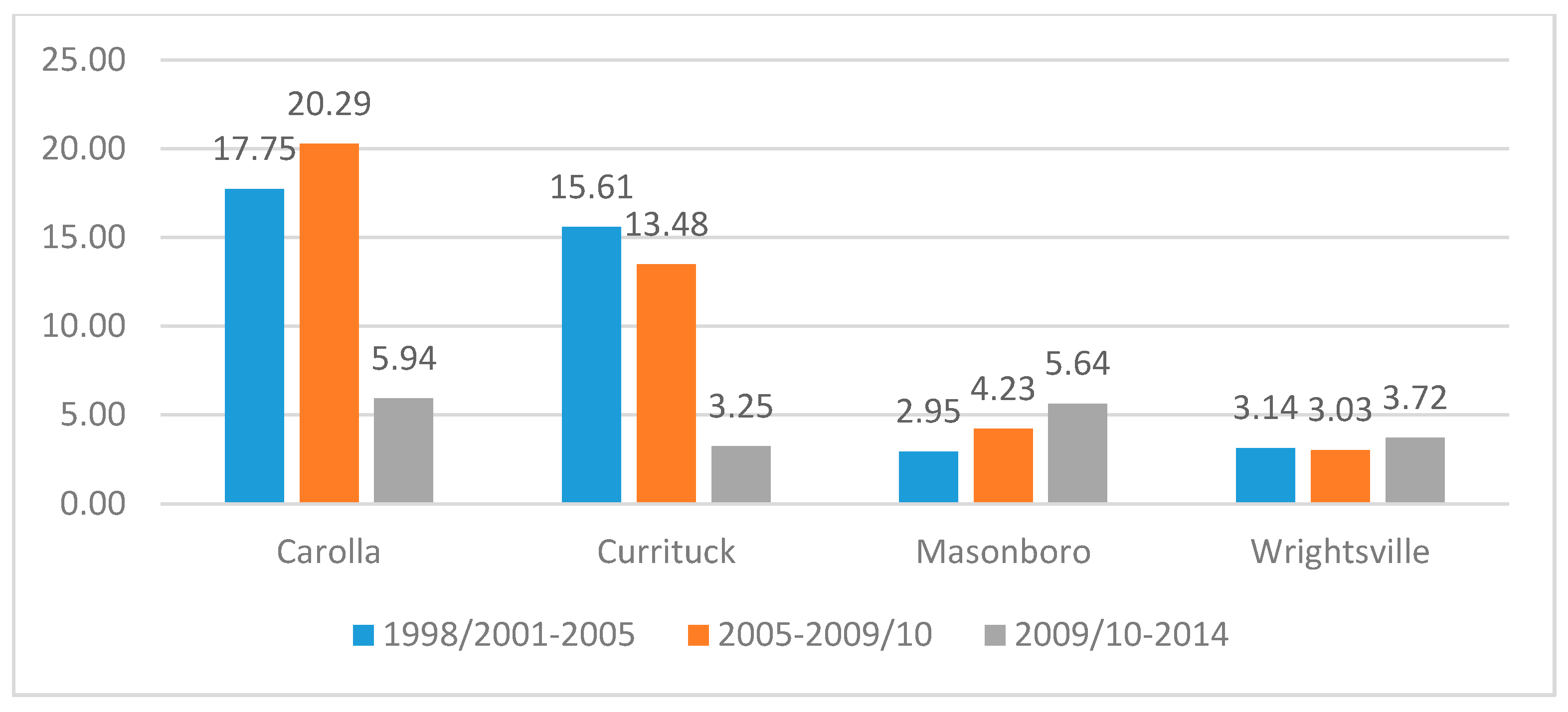
| Corolla | +0.8/2.4 | +2.7/3.5 | −2.7/1.7 |
| Currituck | +0.6/2.0 | +1.5/1.9 | −3.4/1.1 |
| 1998–2005 | 2005–2010 | 2010–2014 | |
| Wrightsville Beach | −0.5/3.5 | +0.5/3.9 | −3.5/1.3 |
| Masonboro Island | −3.1/2.1 | −1.1/1.4 | −1.7/1.1 |
© 2018 by the authors. Licensee MDPI, Basel, Switzerland. This article is an open access article distributed under the terms and conditions of the Creative Commons Attribution (CC BY) license (http://creativecommons.org/licenses/by/4.0/).
Share and Cite
Halls, J.N.; Frishman, M.A.; Hawkes, A.D. An Automated Model to Classify Barrier Island Geomorphology Using Lidar Data and Change Analysis (1998–2014). Remote Sens. 2018, 10, 1109. https://doi.org/10.3390/rs10071109
Halls JN, Frishman MA, Hawkes AD. An Automated Model to Classify Barrier Island Geomorphology Using Lidar Data and Change Analysis (1998–2014). Remote Sensing. 2018; 10(7):1109. https://doi.org/10.3390/rs10071109
Chicago/Turabian StyleHalls, Joanne N., Maria A. Frishman, and Andrea D. Hawkes. 2018. "An Automated Model to Classify Barrier Island Geomorphology Using Lidar Data and Change Analysis (1998–2014)" Remote Sensing 10, no. 7: 1109. https://doi.org/10.3390/rs10071109
APA StyleHalls, J. N., Frishman, M. A., & Hawkes, A. D. (2018). An Automated Model to Classify Barrier Island Geomorphology Using Lidar Data and Change Analysis (1998–2014). Remote Sensing, 10(7), 1109. https://doi.org/10.3390/rs10071109