Article

Deriving High Spatiotemporal Remote Sensing Images Using Deep Convolutional Network

1
State Key Laboratory of Information Engineering in Surveying, Mapping and Remote Sensing (LIESMARS), Wuhan University, Wuhan 430079, China
2
Center for Spatial Information Science and Systems (CSISS), George Mason University, Fairfax, VA 22030, USA
3
School of Remote Sensing and Information Engineering, Wuhan University, Wuhan 430079, China
4
Hubei Province Engineering Center for Intelligent Geoprocessing (HPECIG), Wuhan 430079, China
5
Collaborative Innovation Center of Geospatial Technology (INNOGST), Wuhan 430079, China
*
Authors to whom correspondence should be addressed.
Remote Sens. 2018, 10(7), 1066; https://doi.org/10.3390/rs10071066
Submission received: 8 May 2018 / Revised: 14 June 2018 / Accepted: 29 June 2018 / Published: 5 July 2018
(This article belongs to the Special Issue Deep Learning for Remote Sensing)

Abstract

:
Due to technical and budget limitations, there are inevitably some trade-offs in the design of remote sensing instruments, making it difficult to acquire high spatiotemporal resolution remote sensing images simultaneously. To address this problem, this paper proposes a new data fusion model named the deep convolutional spatiotemporal fusion network (DCSTFN), which makes full use of a convolutional neural network (CNN) to derive high spatiotemporal resolution images from remotely sensed images with high temporal but low spatial resolution (HTLS) and low temporal but high spatial resolution (LTHS). The DCSTFN model is composed of three major parts: the expansion of the HTLS images, the extraction of high frequency components from LTHS images, and the fusion of extracted features. The inputs of the proposed network include a pair of HTLS and LTHS reference images from a single day and another HTLS image on the prediction date. Convolution is used to extract key features from inputs, and deconvolution is employed to expand the size of HTLS images. The features extracted from HTLS and LTHS images are then fused with the aid of an equation that accounts for temporal ground coverage changes. The output image on the prediction day has the spatial resolution of LTHS and temporal resolution of HTLS. Overall, the DCSTFN model establishes a complex but direct non-linear mapping between the inputs and the output. Experiments with MODerate Resolution Imaging Spectroradiometer (MODIS) and Landsat Operational Land Imager (OLI) images show that the proposed CNN-based approach not only achieves state-of-the-art accuracy, but is also more robust than conventional spatiotemporal fusion algorithms. In addition, DCSTFN is a faster and less time-consuming method to perform the data fusion with the trained network, and can potentially be applied to the bulk processing of archived data.

Graphical Abstract

1. Introduction

The advances in modern sensor technology have greatly expanded the use of remote sensing images in scientific research and in many other life activities of humankind [1,2,3]. However, in practice, there are always some trade-offs in the design of remote sensing instruments due to technical and budget limitations. Satellites which image a wider swath width do have a shorter revisiting period, but this usually decreases the spatial resolution of observed images, and vice versa [4]. Currently, it is not easy to acquire images that have both high spatial and high temporal resolution [5,6]. For example, the widely used Landsat images have enabled a 30-m spatial resolution in the visible and infrared spectral bands since the Landsat 4 was launched in 1982 [7]. The latest Landsat 8 maintains a 30-m resolution in most spectral bands, with a long revisiting period of 16 days (the same as Landsat 4, for data continuity purposes) [7]. Conversely, the MODerate Resolution Imaging Spectroradiometer (MODIS) instruments acquire data only at spatial resolution of 250 to 1000 m in multiple spectral bands, but MODIS provides daily coverage of most parts of our planet [8]. For the purpose of long-time series analysis of high spatial resolution imagery (e.g., vegetation-index-based monitoring of crop condition and anomalies at field scale [9,10], as well as water resource assessment [11]), a single high spatial resolution data source usually cannot meet the requirements of frequent temporal coverage. A number of remote sensing data fusion algorithms have been put forward to address this problem, and research has shown that generating high spatiotemporal data by fusing high spatial resolution images and high temporal resolution images from multiple data sources is a practical approach [12,13].
In the remote sensing domain, spatiotemporal data fusion refers to a class of techniques that merge two or more data sources which share similar spectral ranges to generate high spatiotemporal time-series data and to derive richer information than a single data source can provide. In most cases, one data source has high temporal but low spatial resolution (HTLS), while another has low temporal but high spatial resolution (LTHS). After years of development, the research field of spatiotemporal data fusion has established certain theories and methods, and some of these methods have been applied in practical geoscience analysis with respectable accuracy [13,14,15]. As far as we have considered, the existing spatiotemporal fusion algorithms can be classified into three categories: (1) transformation-based; (2) reconstruction-based; and (3) learning-based [16].
The transformation-based methods employ specialized mathematical transforms, such as wavelet transform [17], to transform data from spatial domain to another domain—typically to a frequency or frequency-equivalent domain. Clear, high-frequency components are then extracted from the transformed LTHS images and are merged with HTLS images using elaborately designed fusion rules. The theoretical basis of this approach is that images in different spaces reveal different types of features, which allows a well-designed algorithm to catch the desired features from specific spaces via appropriate transformations.
The reconstruction-based methods generate composite images from weighted sums of spectrally similar neighboring pixels in the HTLS and LTHS image pairs [16]. At present, most of the spatiotemporal fusion algorithms fall into this category. The reconstruction-based methods can be further subdivided into two major groups: one is based on the ground coverage changes of different temporal images, and another is based on the components of mixed ground material end member fractions. In the first case, a hypothetical relation is established based on the difference or ratio deviation between the HTLS and LTHS image pair at the prediction time and a second image pair at a given reference time. Then, a moving window is employed to scan similar neighboring pixels locally and determine the weights. The final composite image is generated by a weighted sum of neighboring pixels in the moving window combined with the hypothetical relation. A typical example is the spatial and temporal adaptive reflectance fusion model (STARFM) [12]. It uses the differences between HTLS and LTHS to establish a relation, and searches similar neighboring pixels by spectral difference, temporal difference, and location distance. Inspired by STARFM, some other enhanced or improved fusion models have been proposed, such as the spatial and temporal adaptive algorithm for mapping reflectance change (STAARCH) [18], enhanced STARFM (ESTARFM) [5], and other STARFM-based models [19]. In general, the main differences among algorithms of this type are in the designs of HTLS and LTHS relations and in the rules used to determine weights.
The second group attacks the same problem by using spectral unmixing techniques to calculate the end member fraction of mixed ground materials and replacing the corresponding components of HTLS at prediction time according to the the unmixed spectral information derived from LTHS at another given time. Typical examples are the unmixed-based data fusion (UBDF) method [20], the flexible spatiotemporal data fusion (FSDAF) method [21], and spatial attraction models (SAM) [22].
The learning-based methods have grown considerably in recent years. Their approaches employ sparse representation or machine learning techniques to extract some abstract features from volumes of data and then reconstruct the predicted data with the extracted features. The main ideas of the sparse-representation-based data fusion are based on the working hypothesis that the HTLS and LTHS data pairs share the same sparse coefficients. By jointly learning a sparse dictionary from the HTLS and LTHS data pairs, the HTLS images can be reconstructed to high spatial resolution images by sparse encoding algorithms. A typical example is the sparse-representation-based spatiotemporal reflectance fusion model (SPSTFM) [23]. Learning-based methods have received increasing attention and are expected to perform better than the conventional ones because they can gain more information from prior data.
Generally speaking, the key factors of a successful fusion algorithm always lie in the design of activity level measurements and fusion rules [24]. Activity level measurements quantify the information quality contained in raw images [25], and fusion rules describe the process of recognizing the information. Hand-crafted level measurements and fusion rules are usually designed based on some mathematical or physical theories. However, the actual data are usually contaminated with errors and noises, and are not conformant to the theoretical ideal. Although most of the algorithms may perform well for some data with great quality or with some specific characteristics in some geographical areas, they may fail with other data and in other areas. In practice, however, it is difficult to acquire sufficient data without cloud or ice cover for a specific area of interest, so the results of conventional algorithms turn out to be less accurate. Furthermore, in some areas within a specific time period there is little LTHS data left once the cloud-covered data are filtered out. That leaves no choice but to extend the time span between the reference data and prediction data. Unfortunately, this produces output that is very unreliable. Besides, the conventional methods process the data pair-by-pair, pixel-by-pixel—each image pair requires a long time to produce the output. In practical cases, where long-time series data are needed, this processing becomes very time-consuming. In contrast, the learning-based methods take time in the training process, but cost much less time in the prediction phase.
In this paper, the problems associated with conventional methods are addressed by a deep learning approach to find a direct non-linear mapping relation between HTLS and LTHS images. Deep learning is a new branch in machine learning technology, inheriting and extending classical artificial neural network principles to automatically learn features and relations of data via more additional hidden processing layers [26,27]. It is widely used in computer vision, natural language processing, finance, and other areas, and has achieved state-of-the-art results in many fields. The pervasive application of convolutional neural networks (CNNs) in speech recognition and visual object recognition and detection has especially drawn significant attention recently [28,29,30]. The novelty of our approach is that a deep convolutional spatiotemporal fusion network (DCSTFN) is built by integrating convolution and deconvolution layers to improve the accuracy and robustness of fusion compared to conventional algorithms. The activity level measurement and fusion rules are actually learned from actual datasets and presented by the weights in each layer. In our experiment, Landsat 8 Operational Land Imager (OLI) and MODIS surface reflectance images are fed into the model to demonstrate its efficacy. The results show that the proposed DCSTFN method outperforms conventional fusion methods. Another significant aspect of the proposed CNN-based approach is its generality, which means it can be applied to various data sources and has enough robustness to handle the quality variations in input data.
The rest of this paper is organized as follows. Section 2 introduces the whole architecture of the proposed DCSTFN model. Section 3 describes the experiment details and comparisons with other classical fusion methods. Discussion and conclusions are presented in Section 4.

2. Materials and Methods

2.1. CNN Model

In machine learning, CNNs are a class of deep feed-forward neural networks designed and trained to extract hierarchical high-level features from inputs using multiple convolutional layers [26,31]. Thanks to the use of a convolution operator, CNNs have fewer connections and parameters than standard feed-forward networks of similar size. In this case, on the one hand, the training time is greatly reduced, on the other hand, it also substantially improves the accuracy of models in practice [30]. A classic CNN is comprised of one or more convolution layers, a subsampling (or called pooling) layer, finally followed by one or more fully-connected (or called dense) layers to generate prediction. The front convolution layers in a CNN are intended to extract low-level features. More complex high-level features can be automatically extracted by increasing the number of convolution layers. The pooling layer abstracts the raw features from the previous layer, reduces training parameters, and prevents the over-fitting of a model.
Deconvolution is another operator that is often employed in CNN models in certain use scenarios, such as unsupervised learning [32], CNN visualization [33], as well as image segmentation and reconstruction [34,35]. Since deconvolution also acts as a convolution operator where the transformation is applied in the opposite direction of a regular convolution, mathematically, a convolution can be expressed as matrix multiplication and deconvolution is the reverse spatial transformation expressed as multiplication with the transposed filter matrix [36]. For this reason, deconvolution in deep learning actually refers to the transposed convolution or backward convolution.
Originally, CNNs were applied to extract high-level features in the image classification and recognition tasks. Eventually, their applications were extended to the image super-resolution and data fusion domains with direct mapping between input(s) and output [24,37]. Currently, the applications of CNNs on image fusion are being actively explored. For example, a deep CNN model was successfully employed to merge images of the same scene taken with different focal settings to gain more clarity [24]. The accuracy of the pan-sharpening method for panchromatic and multispectral image fusion was increased by using CNN-based models [38,39]. In addition, CNN models have also been used in the fusion of multi-spectral and light detection and ranging (LiDAR) data [40]. However, for the problem of spatiotemporal data fusion, to the best of our knowledge, such studies have not yet been carried out widely.

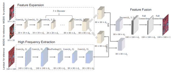
2.2. DCSTFN Architecture

Inspired by the existing work in data fusion models, a deep convolutional fusion network was designed to derive high spatiotemporal resolution remote sensing images. The whole architecture of the DCSTFN can be divided into three parts: the expansion of the HTLS images, the extraction of high-frequency components from LTHS images, and the fusion of extracted features, as shown in Figure 1. The DCSTFN model needs three inputs: the HTLS image at prediction time and an HTLS and LTHS image pair at a time close to the prediction date for reference. The output is the high-resolution image on the prediction date. The two HTLS images go through the shared sub-network on the upper-left. Meanwhile, the reference LTHS image flows past the sub-network on the lower-left. Next, the extracted features with the same size and dimension are merged together to derive the composite image. The arrows in Figure 1 stand for hidden processing layers, and the cubes represent the output tensors (namely multi-dimensional arrays) of each layer. The shape of the cube denotes the size and dimension of the tensor output from the previous layer in the network. Taking the MODIS and Landsat OLI data as an example, the MODIS data are resampled from 500 to 480 m, and the Landsat 8 OLI data remain at 30-m resolution. Thus, the spatial resolution of resampled MODIS data are sixteen times coarser than Landsat OLI. In the training phase, to reduce memory consumption, images are normally divided into smaller patches that can be fed into the network. If we assume the size of each MODIS image patch is 10 × 10 , then the size of a Landsat patch is 160 × 160 . Although images are divided into small patches during training, the input image size for prediction is absolutely not affected once the training process is completed. Besides, considering the large differences in ground surface reflectance from different spectral bands, a single image band should fed into the model to train its own weighted network. The training on the images from different bands will generate different networks under the common DCSTFN architecture. More details are discussed further below.
First, a shared network is used for the HTLS image expansion. This sub-network consists of two convolution layers, three deconvolution layers, and another convolution layer. The two MODIS images both go through the sub-network to extract the low-frequency components and meanwhile expand their input size, respectively. The extracted features will provide the main frame and the background for the fusion result. In Figure 1, the two parameters of a convolution operator denote the number of feature maps and the size of the convolution window, respectively. The number of feature maps is undetermined parameters in a convolution, and the moving window was set to 3 × 3 empirically in our experiment. A rectified linear unit (ReLU) [41] activation function is used for each convolution or deconvolution layer in DCSTFN because ReLU is a commonly-used activation in mainstream CNN models and has achieved excellent results in practice [42]. The deconvolution layers employed in the shared network can expand the MODIS feature maps to the size of Landsat’s so that the two data sources have the same dimension and size in the fusion phase. The first two parameters in a deconvolution operator are the same as the standard convolution, and the last parameter specifies the stride along the convolution window. The stride of deconvolution in this model is set to 2. Therefore, three deconvolutions in the shared network will expand the size of MODIS feature maps eightfold. As shown in Figure 1, the input size of of the shared network for MODIS is 10 × 10 × 1 , and the output size is 80 × 80 × d 2 .
The second part is the extraction of high-frequency components from LTHS images. This sub-network is a classical convolution network starting with two convolution layers, followed by a max-pooling layer that connects with two more convolution layers. The convolution layers are applied to the Landsat image patches to extract the high spatial frequency information like detailed edges and textures. The pooling layer is used to filter high-frequency information. There are three undetermined parameters d i ( i = 0 , 1 , 2 ) in the DCSTFN model, standing for the number of feature maps in three levels of abstraction. These parameters need to be tested and determined with practical experimentation. From Figure 1, the output size of this sub-network for Landsat shrinks from 160 × 160 × 1 to 80 × 80 × d 2 , which is the same as the output size of the sub-network for MODIS.
The last part is the fusion of extracted feature maps from HTLS and LTHS images. A significant difference that distinguishes the DCSTFN model from conventional methods is that our fusion process is performed on the extracted abstract features, while most of the conventional algorithms conduct the fusion based on the original spectral signatures. In the preceding two sub-networks, the features from HTLS and LTHS inputs have coordinated with the same size and dimension. To merge the extracted features, a hypothetical equation from the STARFM model is adopted here. This equation defines the temporal ground coverage changes between HTLS and LTHS images from the reference time t k to the prediction time t 0 , and it can be formulated as follows:
L T H S ( t 0 ) = H T L S ( t 0 ) + L T H S ( t k ) H T L S ( t k ) .
Following this equation, the MODIS patches for reference at time t k are subtracted from Landsat patches for reference on the same day, then the differences are added to the MODIS patches for prediction at time t 0 . At this point, the high and low spatial frequency information extracted from Landsat and MODIS is merged. Then, a deconvolution layer is used to restore the merged patches to the original Landsat data size ( 160 × 160 ). Finally, two fully-connected layers are used to fine-tune the fusion output from the previous layer and reduce the output tensor dimension to restore the fine resolution image. The number of feature maps for the two full connections are set to d 0 and 1 respectively. Notably, the last fully-connected layer is just a linear transformation without any activation operation.

3. Experiment and Evaluation

3.1. Data Preparation

The data collected for the experiment came from the Landsat 8 OLI level-2 surface reflectance product, and from the MODIS surface reflectance 8-day L3 global 500 m (MOD09A1) product. The MODIS daily product naturally has a stronger correlation with the Landsat OLI data of the very same day than the 8-day’s, and thus using the MODIS daily product should theoretically generate a better result. The MODIS 8-day composite product was chosen in our experiment because the daily product has poor data quality, while the 8-day composite product shows much better quality as clouds have been removed as much as possible, missing data have been repaired, and each pixel contains the best possible observation during the 8-day composition period. Based on these considerations, this experiment used the MODIS 8-day product to test our model. In study areas where good-quality daily data are available, the DCSTFN model is totally applicable for the daily data. The initial preprocessing steps that must be performed for the image data are: radiometric calibration, geometric correction, and atmospheric correction. For level-2 products, these processes are done when the data are published. The two data sources are then reprojected into the same map projection and cropped to the same extent. In this experiment, each scene of Landsat images was cropped to the size of 4800 × 4800 by removing the “nodata” pixels from their boundaries. MODIS images are reprojected to the same Universal Transverse Mercator (UTM) projection system used by Landsat. Then, the MODIS data should be cropped to have the same geographical extent as the Landsat (size of 300 × 300 ). A detailed data preprocessing flow chart is shown in Figure 2.
The study area was in the south of Guangdong province, China. The coordinates of the selected area in the Landsat Worldwide Reference System (WRS) were P122R043, P122R044, and P123R044, respectively. The corresponding coordinate to Landsat coverage in the MODIS Sinusoidal Tile Grid was h28v06. Images acquired from January 2013 to December 2017 with less than 10% cloud coverage were collected for this experiment. After the preprocessing, MODIS and Landsat data pairs for reference and prediction were organized in order. Each data group contained four images: a pair of MODIS and Landsat on the prediction date, and a pair on a specific date close to the prediction for reference. The basic rule for data grouping is that the date for reference data should be as close to the prediction data as possible. Since Guangdong is located in the subtropical zone with a humid climate, the acquired satellite images were often covered by ample clouds. If the time span between reference and prediction pairs was longer than two months, we searched the previous or next years to find appropriate reference data as close to the prediction data as possible within the same season. The DCSTFN training process is a type of supervised learning. Three images including Landsat for reference and MODIS for reference and prediction are entered into the model, and the observed Landsat image for prediction is the expected output that guides the direction of the training process.

3.2. Experiment

The DCSTFN model is implemented using Python programming language and the Keras [43] deep learning library with TensorFlow [44] as the computation backend. Keras provides simple, high-level Application Programming Interfaces (APIs) enabling rapid prototyping. There are three undetermined hyper-parameters d i ( i = 0 , 1 , 2 ) in the DCSTFN model, namely the number of feature maps in three abstraction levels. If these numbers are too large, the training process will take a long time doing computation, but if they are too small, the model will not acquire enough knowledge from the training data. Based on the previous CNN-based applications, the three parameters in our experiment were set to 32, 64, and 128, respectively. In this case, the learning network had 408,961 trainable weight parameters in total. The optimization algorithm used for training is called Adam [45], an improved stochastic gradient descent (SGD) method, and has been widely adopted in CNN training. The initial learning rate of Adam was set to 10 3 , β 1 = 0.9 , β 2 = 0.999 , and the decay of the learning rate was set to 10 5 . The loss function used for optimization is mean squared error (MSE), which represents the average of the squares of deviations between predicted values and true values. To contribute to the geoscience community, the implementation code and the trained network were released in open-source format and can be publicly accessed via GitHub (https://github.com/theonegis/rs-data-fusion).
In the training process, eleven image groups from January 2013 to December 2015 were selectively fed into the DCSTFN model for training, and another six groups from January 2016 to December 2017 were chosen for validation. The validation data do not participate in the training. The size of the MODIS image patch was cropped to 10 × 10 , and the cropping stride was set to 5. In our experiment, 320 patches were fed into the model in each training batch. Usually, a larger batch size tends to generate better results. This configuration can be adjusted according to the available hardware context. In the prediction period, an entire image can be entered into the trained network and directly to get the output—regardless of the image patch size in the training period.
When training the network, a single epoch ingests the entire set of samples. As the number of epochs increases, the model can be trained more accurately. After entering the three different bands of data to the DCSTFN model each time, the weights of the network are optimized respectively. Figure 3 shows the evolution of losses during a 50-epoch training period. The line color indicates different spectral bands, and the line style denotes training and validation periods. Figure 4 uses the coefficient of determination ( R 2 ) to represent the predicted results. The R 2 is a statistical measure of how close the data are fitted to the regression function. It is defined as follows:
R 2 = 1 i = 1 N ( y i y ^ ) 2 i = 1 N ( y i y ¯ i ) 2 ,
where y i and y ^ i are the observed and predicted values for the ith pixel values, y ¯ denotes the mean of the observed values, and N is the number of pixels. R 2 often ranges from 0 to 1, but it might be negative if the fit is much worse. The closer it is to 1, the better the prediction.
The following conclusions can be drawn from the training process: (1) The losses of the DCSTFN model did not change significantly after 40 epochs and the network was considered converged; (2) The images of green spectral band had the smallest losses, closely followed by the red band, and the images of the near-infrared (NIR) band had the highest losses; (3) The validation losses were slightly higher than the training losses, and the R 2 of the validation data was slightly lower (less than 0.1) than the training data. This is normal, because the model learned enough features from the training data but had no knowledge about the validation data. However, a good model should produce an accurate prediction for unknown data using the knowledge from the existing data; (4) From the perspective of the coefficient of determination, the DCSTFN model showed the best fitness for red band images in that the R 2 was slightly higher and steadier than the other two. For NIR images, the model did not perform as well as the other two; (5) Although the NIR band had a higher loss than the other bands, the R 2 for NIR band was just slightly lower than others. This is because the NIR band has a wider value range than visible bands. Generally, the prediction results for the NIR band matched observations.

3.3. Comparison

To evaluate the proposed DCSTFN model, two conventional algorithms, including STARM and FSDAF, were compared to the DCSTFN model. STARFM accepts at least one reference image pair, while FSDAF and DCSTFN need only one reference pair. In our experiments, the input images for reference were limited to a single pair so that all of the evaluated algorithms had the same number of inputs. The actual observed Landsat data on the predicted days were used to evaluate the fusion results. By comparing the prediction results and observed data, some statistical metrics were used to obtain the final quantified evaluation results. In addition to the aforementioned R 2 , the root-mean-square error (RMSE), a common measurement of the differences between actual values and predictions, was also used. RMSE is defined as follows:
R M S E = i = 1 N ( y i y ^ i ) 2 N .
The symbols in this formula have the same meanings as for the calculation of R 2 . A smaller RMSE means a better result.
The third index employed to comprehensively evaluate the predictability of the proposed models is the Kling–Gupta efficiency (KGE) [46]. It is defined as follows:
K G E = 1 ( r 1 ) 2 + ( σ y ^ σ y 1 ) 2 + ( μ y ^ μ y 1 ) 2 ,
where r is the correlation coefficient between predicted and observed values, σ y ^ and σ y denote the standard deviation of the predicted and observed values, and μ y ^ and μ y denote the mean value of the predicted and observed values. The KGE of an ideal result is 1.
The last is the structural similarity (SSIM) index [47], which is often used to measure the similarity between the actual and predicted images visually. It is defined as follows:
S S I M = ( 2 μ y μ y ^ + C 1 ) ( 2 σ y y ^ + C 2 ) ( μ y 2 + μ y ^ 2 + C 1 ) ( σ y 2 + σ y ^ 2 + C 2 ) ,
where σ y y ^ denotes the covariance between the observed and predicted values, and C 1 and C 2 are the constants to enhance the stability of SSIM. The value of SSIM ranges from −1 to 1. The closer it is to 1, the more similar two images are.
Three scenes of images from the validation dataset were used to perform the evaluation: (1) prediction on 7 December 2016 with reference on 5 November 2016 in P122R043; (2) prediction on 23 October 2017 with reference on 7 December 2016 in P122R044; (3) prediction on 1 March 2016 with reference on 16 April 2015 in P123R044. The quantitative evaluations in terms of RMSE, R 2 , KGE, and SSIM for the fusion results are listed in Table 1, Table 2 and Table 3, respectively. The surface reflectance values in the following were all scaled by 10,000, as with the image pixel values. We can obtain following information from the tables: (1) For the DCSTFN model, overall the R 2 metrics were greater than 0.9 for the three bands; the KGE indices were greater than 0.8; and the SSIM indices were greater than 0.9. (2) Most metrics of DCSTFN were better than conventional methods, but a few were not. For example, the RMSEs of STARFM were slightly smaller than DCSTFN for some bands in a specific scene. (3) From the comprehensive evaluation of the prediction model, KGE indices for DCSTFN were all better than the others and remained stable. From the visual inspection of the output images, SSIM indices for DCSTFN showed a higher similarity than others. (4) The KGE of STARFM was not stable, which shows that the input data quality had a great influence on the STARFM algorithm. The poor KGE may be caused by the fact that there were some “nodata” pixels in the output of STARFM. In contrast, the DCSTFN was very robust and not very sensitive to the input data quality.
Figure 5 illustrates the fusion results on 7 December 2016 with reference on 5 November 2016 in P122R043 from different models. The first row presents the overviews of the scene from different models, and the second row corresponds to the yellow rectangles in the first row. The images of the first two rows are standard false color composite. The last row shows the calculated Normalized Difference Vegetation Index (NDVI) which is an important indicator that is frequently used in remote sensing analysis to quantify vegetation. From Figure 5, it can be intuitively seen from the first row that in general the DCSTFN result was slightly closer to the actual observation. The overall image tone of STARFM and FSDAF appeared darker than the observed image, especially on the upper-left. Second, there were some “nodata” pixels in the STARFM result because of the poor input data quality, as shown in the green rectangle, which does not exist in the DCSTFN model. Third, since the input Landsat image on 5 November 2016 was covered by small amount of clouds in the lower-right corner corresponding to the orange rectangles, the fusion results were of course contaminated by clouds. However, the DCSTFN result was the least affected among the three. Fourth, from the second row, it can be seen that STARFM and FSDAF failed to catch the ground details of the urban area with heterogeneous features marked with magenta rectangles, but the DCSTFN worked quite well. Fifth, the NDVI image derived from DCSTFN output was apparently the closest to the actual observation, and detailed information can be seen clearly. Hence, a conclusion can be safely drawn from Figure 5 that the DCSTFN model was more robust than conventional methods regardless of the input data quality, and the results contained more details and showed a higher accuracy. Note that the existing spatiotemporal fusion algorithms share the disadvantage that the reference data have a significant impact on the prediction. Because the spatial resolution of the coarse MODIS data need to be amplified sixteen times to match Landsat’s, much of the information needs to be referred from the reference data. Inevitably, both the data quality of reference data and the degree of ground changes between the reference and prediction date can influence the fusion result. Nevertheless, the DCSTFN model less affected than the other two.
Figure 6 shows plots of the observed and predicted surface reflectance. The figure intuitively demonstrates how the prediction results from different models fit into the actual observation. The samples come from the the upper-left corner of the whole-scene images in Figure 5 ( 500 × 500 ). The color in the plots indicates the density of points. For the visible bands, the R 2 of DCSTFN was slightly larger than STARFM and FDSAF, and points far from the real values were less than the other two, which means that the prediction error rate of DCSTFN was lower. For the NIR band, the “point cloud” of DCSTFN was clearly narrower than the other two, which shows a higher correlation. In conclusion, both statistical metrics and visual inspection of the correlation plots show that the results of DCSTFN were closer to the actual observations than the other two.

4. Conclusions and Future Work

This paper introduces the deep learning approach into the remote sensing spatiotemporal data fusion domain and produces a state-of-the-art result. The advantages of our CNN-based fusion approach are twofold: (1) it can generate series of high spatiotemporal resolution images with high accuracy and it is more robust and less-sensitive to the input data quality than conventional methods; and (2) the DCSTFN model can save more time when handling large volumes of data for a long-time series analysis. Once the network is established, it can be used for the entire dataset. In contrast, conventional methods are more suitable for tasks where input data are of relatively good quality and the data volumes to be processed are not too large. We also made our implementation code and trained network publicly accessible. Users can train on other areas with their datasets based on our results without starting from scratch.
We believe that future work with regard to the DCSTFN model should proceed in two directions. First, some tuning practices from deep learning should be applied to the DCSTFN model to explore performance improvements. For example, batch normalization [48] can be added into the layers of the network to reduce overfitting. The idea of a residual network [49] can be introduced into the DCSTFN model to address the degradation of the deep learning network. Second, a case study of practical analysis should be conducted to evaluate whether the model can satisfy practical needs. Moreover, we want to utilize the deep learning approach to explore the possibility of generating high spatiotemporal resolution images with only a single HTLS image in the prediction period. To the best of our knowledge, existing spatiotemporal fusion algorithms all need at least one HSLT and HTLS pair for reference. Inappropriate reference data can greatly influence the accuracy of the fusion result. However, it is often not easy to find high-quality reference images because of cloud or ice cover in the study area. For this reason, we want to explore the possibility of using learned prior knowledge from the HSLT images in the training period and then using the learned features and relational mapping to derive the fusion result with only one HTLS image on the prediction day. If this is achieved, it will greatly promote the use of the spatiotemporal fusion method in practical applications.

Author Contributions

Z.T., L.D. and P.Y. designed the method; Z.T. conducted the experiment and wrote the paper; Z.T. and J.T. performed data preprocessing; L.D. and P.Y. revised the manuscript.

Funding

This research was partially supported by a grant from the U.S. National Science Foundation (Grant #: CNS-1739705, PI: Dr. Liping Di), Major State Research Development Program of China (No. 2017YFB0503704), National Natural Science Foundation of China (No. 41722109),and Wuhan Yellow Crane Talents (Science) Program.

Conflicts of Interest

The authors declare no conflict of interest.

Abbreviations

MODISMODerate Resolution Imaging Spectroradiometer
OILOperational Land Imager
HTLShigh temporal but low spatial resolution
LTHSlow temporal but high spatial resolution
STARFMspatial and temporal adaptive reflectance fusion model
STAARCHspatial and temporal adaptive algorithm for mapping reflectance change
ESTARFMenhanced spatial and temporal adaptive reflectance fusion model
UBDFunmixed-based data fusion
FSDAFflexible spatiotemporal data fusion
SAMspatial attraction model
SPSTFMsparse-representation-based spatiotemporal reflectance fusion model
CNNconvolutional neural network
DCSTFNdeep convolutional spatiotemporal fusion network
LiDARlight detection and ranging
ReLUrectified linear unit
UTMUniversal Transverse Mercator
SGDstochastic gradient descent
NIRnear-infrared
RMSEroot-mean-square error
KGEKling–Gupta efficiency
SSIMstructural similarity index
NDVINormalized Difference Vegetation Index

References

  1. Toth, C.; Jóźków, G. Remote sensing platforms and sensors: A survey. ISPRS J. Photogramm. Remote Sens. 2016, 115, 22–36. [Google Scholar] [CrossRef]
  2. Di, L.; Moe, K.; van Zyl, T.L. Earth Observation Sensor Web: An Overview. IEEE J. Sel. Top. Appl. Earth Obs. Remote Sens. 2010, 3, 415–417. [Google Scholar] [CrossRef]
  3. Di, L. Geospatial sensor web and self-adaptive Earth predictive systems (SEPS). In Proceedings of the Earth Science Technology Office (ESTO)/Advanced Information System Technology (AIST) Sensor Web Principal Investigator (PI) Meeting, San Diego, CA, USA, 13–14 February 2007; pp. 1–4. [Google Scholar]
  4. Alavipanah, S.; Matinfar, H.; Rafiei Emam, A.; Khodaei, K.; Hadji Bagheri, R.; Yazdan Panah, A. Criteria of selecting satellite data for studying land resources. Desert 2010, 15, 83–102. [Google Scholar]
  5. Zhu, X.; Chen, J.; Gao, F.; Chen, X.; Masek, J.G. An enhanced spatial and temporal adaptive reflectance fusion model for complex heterogeneous regions. Remote Sens. Environ. 2010, 114, 2610–2623. [Google Scholar] [CrossRef]
  6. Patanè, G.; Spagnuolo, M. Heterogeneous Spatial Data: Fusion, Modeling, and Analysis for GIS Applications. Synth. Lect. Vis. Comput. Comput. Gr. Anim. Comput. Photogr. Imag. 2016, 8, 1–155. [Google Scholar]
  7. Roy, D.P.; Wulder, M.A.; Loveland, T.R.; Woodcock, C.E.; Allen, R.G.; Anderson, M.C.; Helder, D.; Irons, J.R.; Johnson, D.M.; Kennedy, R.; et al. Landsat-8: Science and product vision for terrestrial global change research. Remote Sens. Environ. 2014, 145, 154–172. [Google Scholar] [CrossRef]
  8. Justice, C.O.; Vermote, E.; Townshend, J.R.G.; Defries, R.; Roy, D.P.; Hall, D.K.; Salomonson, V.V.; Privette, J.L.; Riggs, G.; Strahler, A.; et al. The Moderate Resolution Imaging Spectroradiometer (MODIS): Land remote sensing for global change research. IEEE Trans. Geosci. Remote Sens. 1998, 36, 1228–1249. [Google Scholar] [CrossRef]
  9. Deng, M.; Di, L.; Han, W.; Yagci, A.L.; Peng, C.; Heo, G. Web-service-based Monitoring and Analysis of Global Agricultural Drought. Photogramm. Eng. Remote Sens. 2013, 79, 929–943. [Google Scholar] [CrossRef]
  10. Yang, Z.; Di, L.; Yu, G.; Chen, Z. Vegetation condition indices for crop vegetation condition monitoring. In Proceedings of the 2011 IEEE International Geoscience and Remote Sensing Symposium, Vancouver, BC, Canada, 24–29 July 2011; pp. 3534–3537. [Google Scholar]
  11. Nair, H.C.; Padmalal, D.; Joseph, A.; Vinod, P.G. Delineation of Groundwater Potential Zones in River Basins Using Geospatial Tools—An Example from Southern Western Ghats, Kerala, India. J. Geovisualiz. Spat. Anal. 2017, 1, 5. [Google Scholar] [CrossRef]
  12. Gao, F.; Masek, J.; Schwaller, M.; Hall, F. On the blending of the Landsat and MODIS surface reflectance: predicting daily Landsat surface reflectance. IEEE Trans. Geosci. Remote Sens. 2006, 44, 2207–2218. [Google Scholar] [CrossRef]
  13. Hilker, T.; Wulder, M.A.; Coops, N.C.; Seitz, N.; White, J.C.; Gao, F.; Masek, J.G.; Stenhouse, G. Generation of dense time series synthetic Landsat data through data blending with MODIS using a spatial and temporal adaptive reflectance fusion model. Remote Sens. Environ. 2009, 113, 1988–1999. [Google Scholar] [CrossRef]
  14. Emelyanova, I.V.; McVicar, T.R.; Niel, T.G.V.; Li, L.T.; van Dijk, A.I. Assessing the accuracy of blending Landsat–MODIS surface reflectances in two landscapes with contrasting spatial and temporal dynamics: A framework for algorithm selection. Remote Sens. Environ. 2013, 133, 193–209. [Google Scholar] [CrossRef]
  15. Li, X.; Ling, F.; Foody, G.M.; Ge, Y.; Zhang, Y.; Du, Y. Generating a series of fine spatial and temporal resolution land cover maps by fusing coarse spatial resolution remotely sensed images and fine spatial resolution land cover maps. Remote Sens. Environ. 2017, 196, 293–311. [Google Scholar] [CrossRef] [Green Version]
  16. Chen, B.; Huang, B.; Xu, B. Comparison of Spatiotemporal Fusion Models: A Review. Remote Sens. 2015, 7, 1798–1835. [Google Scholar] [CrossRef] [Green Version]
  17. Acerbi-Junior, F.; Clevers, J.; Schaepman, M. The assessment of multi-sensor image fusion using wavelet transforms for mapping the Brazilian Savanna. Int. J. Appl. Earth Obs. Geoinf. 2006, 8, 278–288. [Google Scholar] [CrossRef]
  18. Hilker, T.; Wulder, M.A.; Coops, N.C.; Linke, J.; McDermid, G.; Masek, J.G.; Gao, F.; White, J.C. A new data fusion model for high spatial- and temporal-resolution mapping of forest disturbance based on Landsat and MODIS. Remote Sens. Environ. 2009, 113, 1613–1627. [Google Scholar] [CrossRef]
  19. Shen, H.; Wu, P.; Liu, Y.; Ai, T.; Wang, Y.; Liu, X. A spatial and temporal reflectance fusion model considering sensor observation differences. Int. J. Remote Sens. 2013, 34, 4367–4383. [Google Scholar] [CrossRef]
  20. Zurita-Milla, R.; Clevers, J.G.P.W.; Schaepman, M.E. Unmixing-Based Landsat TM and MERIS FR Data Fusion. IEEE Geosci. Remote Sens. Lett. 2008, 5, 453–457. [Google Scholar] [CrossRef] [Green Version]
  21. Zhu, X.; Helmer, E.H.; Gao, F.; Liu, D.; Chen, J.; Lefsky, M.A. A flexible spatiotemporal method for fusing satellite images with different resolutions. Remote Sens. Environ. 2016, 172, 165–177. [Google Scholar] [CrossRef]
  22. Lu, L.; Huang, Y.; Di, L.; Hang, D. A New Spatial Attraction Model for Improving Subpixel Land Cover Classification. Remote Sens. 2017, 9, 360. [Google Scholar] [CrossRef]
  23. Huang, B.; Song, H. Spatiotemporal Reflectance Fusion via Sparse Representation. IEEE Trans. Geosci. Remote Sens. 2012, 50, 3707–3716. [Google Scholar] [CrossRef]
  24. Liu, Y.; Chen, X.; Peng, H.; Wang, Z. Multi-focus image fusion with a deep convolutional neural network. Inf. Fusion 2017, 36, 191–207. [Google Scholar] [CrossRef]
  25. Blum, R.S.; Liu, Z. Multi-Sensor Image Fusion and Its Applications; CRC Press: Boca Raton, FL, USA, 2005. [Google Scholar]
  26. LeCun, Y.; Bengio, Y.; Hinton, G. Deep learning. Nature 2015, 521, 436–444. [Google Scholar] [CrossRef] [PubMed]
  27. Schmidhuber, J. Deep learning in neural networks: An overview. Neural Netw. 2015, 61, 85–117. [Google Scholar] [CrossRef] [PubMed] [Green Version]
  28. Liu, W.; Wang, Z.; Liu, X.; Zeng, N.; Liu, Y.; Alsaadi, F.E. A survey of deep neural network architectures and their applications. Neurocomputing 2017, 234, 11–26. [Google Scholar] [CrossRef]
  29. Kim, Y. Convolutional neural networks for sentence classification. arXiv, 2014; arXiv:1408.5882. [Google Scholar]
  30. Krizhevsky, A.; Sutskever, I.; Hinton, G.E. ImageNet Classification with Deep Convolutional Neural Networks. In Advances in Neural Information Processing Systems; Pereira, F., Burges, C.J.C., Bottou, L., Weinberger, K.Q., Eds.; Curran Associates, Inc.: New York, NY, USA, 2012; Volume 25, pp. 1097–1105. [Google Scholar]
  31. LeCun, Y.; Bengio, Y. Convolutional networks for images, speech, and time series. Handb. Brain Theory Neural Netw. 1995, 3361, 1995. [Google Scholar]
  32. Zeiler, M.D.; Taylor, G.W.; Fergus, R. Adaptive deconvolutional networks for mid and high level feature learning. In Proceedings of the 2011 International Conference on Computer Vision, Barcelona, Spain, 6–13 November 2011; pp. 2018–2025. [Google Scholar]
  33. Zeiler, M.D.; Fergus, R. Visualizing and Understanding Convolutional Networks. In Computer Vision—ECCV 2014; Fleet, D., Pajdla, T., Schiele, B., Tuytelaars, T., Eds.; Springer International Publishing: Cham, Switzerland, 2014; pp. 818–833. [Google Scholar]
  34. Shelhamer, E.; Long, J.; Darrell, T. Fully Convolutional Networks for Semantic Segmentation. IEEE Trans. Pattern Anal. Mach. Intell. 2017, 39, 640–651. [Google Scholar] [CrossRef] [PubMed]
  35. Radford, A.; Metz, L.; Chintala, S. Unsupervised representation learning with deep convolutional generative adversarial networks. arXiv, 2015; arXiv:1511.06434. [Google Scholar]
  36. Dumoulin, V.; Visin, F. A guide to convolution arithmetic for deep learning. arXiv, 2016; arXiv:1603.07285. [Google Scholar]
  37. Dong, C.; Loy, C.C.; He, K.; Tang, X. Image Super-Resolution Using Deep Convolutional Networks. IEEE Trans. Pattern Anal. Mach. Intell. 2016, 38, 295–307. [Google Scholar] [CrossRef] [PubMed]
  38. Masi, G.; Cozzolino, D.; Verdoliva, L.; Scarpa, G. Pansharpening by Convolutional Neural Networks. Remote Sens. 2016, 8, 594. [Google Scholar] [CrossRef]
  39. Wei, Y.; Yuan, Q.; Shen, H.; Zhang, L. Boosting the Accuracy of Multispectral Image Pansharpening by Learning a Deep Residual Network. IEEE Geosci. Remote Sens. Lett. 2017, 14, 1795–1799. [Google Scholar] [CrossRef] [Green Version]
  40. Chen, Y.; Li, C.; Ghamisi, P.; Jia, X.; Gu, Y. Deep Fusion of Remote Sensing Data for Accurate Classification. IEEE Geosci. Remote Sens. Lett. 2017, 14, 1253–1257. [Google Scholar] [CrossRef]
  41. Nair, V.; Hinton, G.E. Rectified Linear Units Improve Restricted Boltzmann Machines. In Proceedings of the 27th International Conference on International Conference on Machine Learning (ICML’10), Madison, WI, USA, 21–24 June 2010; pp. 807–814. [Google Scholar]
  42. Zhu, X.X.; Tuia, D.; Mou, L.; Xia, G.S.; Zhang, L.; Xu, F.; Fraundorfer, F. Deep Learning in Remote Sensing: A Comprehensive Review and List of Resources. IEEE Geosci. Remote Sens. Mag. 2017, 5, 8–36. [Google Scholar] [CrossRef] [Green Version]
  43. Chollet, F. Keras. 2015. Available online: https://github.com/keras-team/keras (accessed on 29 June 2018).
  44. Abadi, M.; Barham, P.; Chen, J.; Chen, Z.; Davis, A.; Dean, J.; Devin, M.; Ghemawat, S.; Irving, G.; Isard, M.; et al. TensorFlow: A System for Large-Scale Machine Learning. OSDI 2016, 16, 265–283. [Google Scholar]
  45. Kingma, D.P.; Ba, J. Adam: A method for stochastic optimization. arXiv, 2014; arXiv:1412.6980. [Google Scholar]
  46. Gupta, H.V.; Kling, H.; Yilmaz, K.K.; Martinez, G.F. Decomposition of the mean squared error and NSE performance criteria: Implications for improving hydrological modelling. J. Hydrol. 2009, 377, 80–91. [Google Scholar] [CrossRef] [Green Version]
  47. Wang, Z.; Bovik, A.C.; Sheikh, H.R.; Simoncelli, E.P. Image quality assessment: from error visibility to structural similarity. IEEE Trans. Image Process. 2004, 13, 600–612. [Google Scholar] [CrossRef] [PubMed]
  48. Ioffe, S.; Szegedy, C. Batch normalization: Accelerating deep network training by reducing internal covariate shift. arXiv, 2015; arXiv:1502.03167. [Google Scholar]
  49. He, K.; Zhang, X.; Ren, S.; Sun, J. Deep residual learning for image recognition. In Proceedings of the IEEE Conference on Computer Vision and Pattern Recognition, Las Vegas, NV, USA, 26 June–1 July 2016; pp. 770–778. [Google Scholar]
Figure 1. The architecture of the deep convolutional spatiotemporal fusion network (DCSTFN) model.
Remotesensing 10 01066 g001
Figure 2. The flow chart of data preprocessing. MODIS: MODerate Resolution Imaging Spectroradiometer; UTM: Universal Transverse Mercator.
Remotesensing 10 01066 g002
Figure 3. Losses of the DCSTFN model. MSE: mean squared error; NIR: near-infrared.
Remotesensing 10 01066 g003
Figure 4. Fitness of the DCSTFN model.
Remotesensing 10 01066 g004
Figure 5. Illustration of data fusion results from different models on 7 December 2016 in P122R043. NDVI: Normalized Difference Vegetation Index.
Remotesensing 10 01066 g005
Figure 6. FSDAF for NIR band
Remotesensing 10 01066 g006
Table 1. The quantitative evaluations for the fusion result on 7 December 2016 in P122R043 (The metrics of DCSTFN are highlighted). FSDAF: flexible spatiotemporal data fusion; KGE: Kling–Gupta efficiency; RMSE: root-mean-square error; SSIM: structural similarity; STARFM: spatial and temporal adaptive reflectance fusion model.
GreenRedNIR
DCSTFNSTARFMFSDAFDCSTFNSTARFMFSDAFDCSTFNSTARFMFSDAF
RMSE65.47070.35070.63258.34865.15865.89958.06446.02045.502
R 2 0.9190.9060.9060.9560.9450.9440.9940.9970.997
KGE0.879−0.9500.6670.901−0.5510.7450.8840.7060.846
SSIM0.9640.9400.9360.9570.7450.9250.9200.8460.890
Table 2. The quantitative evaluations for the fusion result on 23 October 2017 in P122R044.
GreenRedNIR
DCSTFNSTARFMFSDAFDCSTFNSTARFMFSDAFDCSTFNSTARFMFSDAF
RMSE66.11262.63061.10960.43560.40260.17244.88546.35045.912
R 2 0.9710.9740.9750.9840.9840.9840.9980.9980.998
KGE0.8860.5000.7210.8660.1380.7800.8280.4310.847
SSIM0.9090.8720.8670.8800.8220.8290.8090.7830.801
Table 3. The quantitative evaluations for the fusion result on 1 March 2016 in P123R044.
GreenRedNIR
DCSTFNSTARFMFSDAFDCSTFNSTARFMFSDAFDCSTFNSTARFMFSDAF
RMSE60.15966.69664.18361.73766.48865.13549.79644.16043.952
R 2 0.9260.9090.9150.9500.9420.9450.9910.9930.993
KGE0.8700.3680.7510.858−0.2960.7490.740−0.1820.682
SSIM0.9480.9130.9070.9140.8650.8660.7620.6940.718

