Diffuse Attenuation Coefficient Retrieval in CDOM Dominated Inland Water with High Chlorophyll-a Concentrations

Abstract

The k_d(490) is a vertical light attenuation coefficient and an important parameter for water quality. The k_d estimates are often based on empirical and semi-analytical algorithms, designed for oceanic and coastal waters. However, there is a lack of information about the performances of these models to inland waters dominated by chromophoric dissolved organic matter (CDOM). Therefore, to contribute to this investigation, nine empirical models based on the blue-to-green and blue-to-red ratios and chlorophyll-a (Chl-a) concentration were evaluated, as well as three semi-analytical models using bands from the Operational Land Imager (OLI)/Landsat-8. The errors (mean absolute percentage error, MAPE > 80%) presented by the empirical models confirmed that the blue-to-green ratio failed in retrieving k_d(490) in an environment dominated by CDOM. Similar failures occurred with the models using the Chl-a concentration (MAPE ~60%) as input. A semi-analytical approach showed the lowest error (MAPE = 41.04%) in the estimate of the inherent optical properties for complex waters in order to reduce the errors above. After retrieval of k_d(490) using the semi-analytical model, seasonal patterns were observed, and high values of k_d(490) were detected in the dry season possibly due to the increase of the concentration of the optically-significant substances (OSS).

1. Introduction

The diffuse attenuation coefficient (k_d) is an apparent optical property (AOP) and is defined as the exponential decrease of the ambient downwelling irradiance (E_d) with depth and is, therefore, related to light penetration and availability and can be used to predict the euphotic depth. AOPs are those properties that depend both on the medium and on the geometric structure of the radiance distribution [1]. k_d is largely determined by the inherent optical properties (IOPs), absorption (a), and backscattering (b_b) coefficients of the first-order, and are less dependent on the incident radiation field as the sun angle. IOPs are properties of the medium and do not depend on the ambient light field [1].

Non-algal particles (NAP), phytoplankton, chromophoric dissolved organic matter (CDOM), and water itself are considered the four optically-significant substances (OSS) that control the k_d. The k_d at 490 nm, k_d(490), is generally considered and classified as a parameter of water quality and, therefore, is essential for monitoring the eutrophication process due to light attenuation by phytoplankton growth or suspended matter [2]. The capacity of the inverse of k_d(490) to provide the depth from which 90% of the upwelling signal at 490 nm originates allows for the remote estimation. For primary production models, the k_d(490) was used as a surrogate for the attenuation coefficient of photosynthetically-active radiation, k_d(PAR); the significant positive correlation between k_d(490) and k_d(PAR) allowed the k_d(PAR) inference from k_d(490) [3,4]. For monitoring eutrophication and the associated decrease in light attenuation, the accurate estimation of k_d is critical to better understand and model the primary productivity, heat, and gas transfer in aquatic systems.

In order to estimate k_d(490), empirical algorithms were developed using a direct conversion from normalized water-leaving radiance (nL_w) or remote sensing reflectance (R_rs) ratios or indirect conversion through products based on chlorophyll-a (Chl-a) concentrations [3,4,5,6,7,8,9]. However, these models are considered site-specific, which is a limiting factor for broader applications. Wang et al. [9] and Lee et al. [10] came up with a semi-analytical approach covering a wide range of waters. Wang et al. [9] used a combination of two models suitable for ocean and turbid coastal waters, aiming to improve the application range of k_d(490) estimations. The model from Lee et al. [9] considered the IOPs derived from R_rs through a quasi-analytical algorithm (QAA) [11] and the solar zenith angle using the radiative transfer theory. The algorithm makes it possible the estimation of spectral k_d, as well as k_d(490), for water bodies ranging from the clearest ocean to turbid coastal waters.

Even so, studies showing the use of remote sensing for k_d(490) estimation in tropical productive inland waters are hampered by the lack of in situ data and theoretical framework to predict and interpret water color data [12]. The optical complexity of turbid waters (mineral suspended solids, algae, and associated organic particles) produce multiple scattering, hampering the mathematical analysis of radiative transfer [12]. From our understanding there are very few investigations of k_d(490) estimation through the oceanic-based algorithms in inland waters dominated by CDOM, which is an optically-active indicator of dissolved organic matter and plays an important role in cycling carbon.

CDOM is considered an important water quality indicator due to its impact on drinking water, carbon balance, and aquatic ecosystems; mainly because CDOM affects the penetration of light into the water column, which affects the primary productivity. Most models use R_rs or nL_w from the blue-green spectral region, in which the CDOM has high absorption. Due to this, the following questions arise: (1) Will the k_d(490) models that use the blue/green ratio be impacted in such a way that the errors make it impossible to use? (2) How will these models be impacted in the presence of high Chl-a concentrations? (3) Will the semi-analytical models, which use IOPs as the input data, perform better than the empirical ones? (4) What are the potential for k_d monitoring from space in inland waters dominated by CDOM?

Therefore, the main goal of this paper was to assess the performance of algorithms to estimate k_d(490) in inland waters dominated by CDOM, which are widely available to end users. We tested nine empirical and three semi-analytical algorithms. The selected models will help us to answer the above questions.

2. Materials and Methods

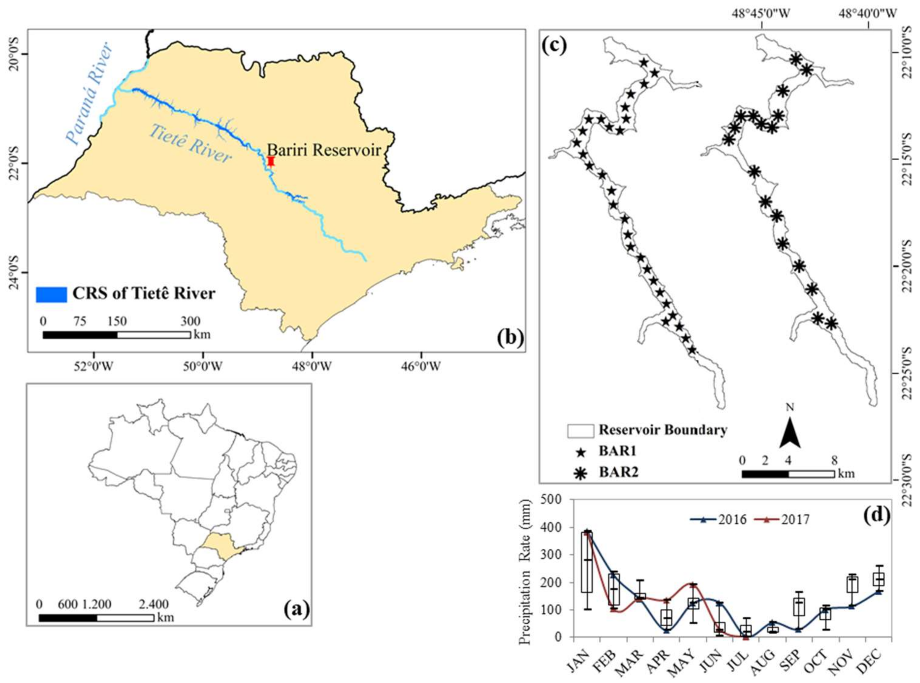
2.1. Study Area and Sampling Planning

The Bariri hydroelectric reservoir (22°9′49.260″ S 48°44′21.420″ W) is in the middle of São Paulo State and is part of the Cascading Reservoir System (CRS) of the Tietê River (Figure 1). Bariri is the second of a total of six reservoirs and presents the smallest flooded area of 63 km² at an average altitude of 450 m. The Bariri reservoir is situated in a tropical climate with a dry period (April–September) and a wet period (October–March) according to the Köppen classification. Water retention time varies between 7 and 24 days [13,14].

The amount of wastewater coming from the metropolitan region of the Tietê River characterizes the Bariri Reservoir as highly productive water with high average concentrations of total nitrogen (2750 μg·L⁻¹), phosphorus (87 μg·L⁻¹), and Chl-a (55.8 μg·L⁻¹) with the phytoplankton community dominated by cyanobacteria.

Two surveys were carried out where, in the first case (BAR1), 30 samples were collected from 15–18 August 2016 and, in the second case (BAR2), 18 samples were taken from 23–24 June 2017 (see Figure 1 for sample locations). The days of the field campaigns were planned with respect to the temporal resolution of OLI/Landsat-8, aiming to match the data collection with the satellite overpass of the study site.

2.2. Water Quality and Optical Data

Wind speed (m s⁻¹), pH, depth (m), Secchi disk depth (Z_SD; m), and turbidity (NTU) were measured in the field with an anemometer, pH meter, depth gauge, Secchi disk, and turbidity meter, respectively. The water samples were collected in the field to derive the OSS, such as the Chl-a and the suspended particulate matter (SPM), as well as the inorganic (IPM) and organic particulate matter (OPM) concentrations according to Golterman et al. [15] and the American Public Health Association Protocol [16], respectively.

The IOP data analysis followed the methodology proposed in Bricaud et al. [17] for the absorption coefficient of the colored dissolved organic matter (a_CDOM). A baseline correction was performed by subtracting the average value between 700 and 750 nm from all the spectrum values; while for the absorption coefficients of non-algal particle (a_NAP) and the total particulate (a_p), that consists in the sum of a_NAP and phytoplankton absorption coefficient (a_φ), the acquisition and analyses were made in accordance with the transmittance-reflectance method, according to Tassan and Ferrari [18,19,20].

The radiometric data were obtained from the two hyperspectral RAMSES sensors (TriOS, Rastede, Germany). The sky and total radiance data (L_sky and L_t, respectively, both in W m⁻² sr⁻¹) and the downwelling and sky irradiance data (E_d and E_sky, respectively, both in W m⁻²) were taken with the sensors fixed by a steel frame in the boat, in a configuration of 40° from nadir (zenith) and to azimuthal angle of 90° in order to minimize the specular reflection [21]. The radiometric quantities were used to calculate the remote sensing reflectance [22] according to Equation (1):

$$R_{rs}\left(\lambda \right)=\frac{L_t\left(\lambda \right)-L_{SR}\left(\lambda \right)}{E_d\left(\lambda \right)}=\frac{L_t\left(\lambda \right)-({\rho }_{sky}\times L_S\left(\lambda \right))}{E_d\left(\lambda \right)}-\mathsf{\Delta }$$

(1)

where L_SR(λ) is the surface-reflected light and consists of a fraction (ρ_sky≈0.02-0.05) of L_S(λ) and the sun glint, residual glint, whitecaps and foam-reflected light ($\mathsf{\Delta }$). The $\mathsf{\Delta }$ value can be assumed to be zero for oceanic water in the near-infrared (NIR); however, in turbid water, this element must be retrieved. In agreement with that, Lee et al. [22] proposed a calculation approach of R_rs as a function of the total remote-sensing reflectance (T_rs, ratio of L_t to E_d) and sky remote-sensing reflectance (S_rs, ratio of L_sky to E_d) for each L_t and L_sky scan from the Equation (2):

$${\mathrm{R}}_{\mathrm{rs}}\left(\mathsf{\lambda }\right)\approx {\mathrm{T}}_{\mathrm{rs}}\left(\mathsf{\lambda }\right)-\mathrm{F}\times {\mathrm{S}}_{\mathrm{rs}}\left(\mathsf{\lambda }\right)-\mathsf{\Delta }$$

(2)

where $\mathsf{\Delta }$ is spectrally constant, settled before ${\mathrm{R}}_{\mathrm{rs}}$ can be derived [22]. F is the surface Fresnel reflectance based on the viewing geometry (~0.021), and ${\mathrm{S}}_{\mathrm{rs}}\left(\mathsf{\lambda }\right)$ is the sky remote sensing reflectance. The value of $\mathsf{\Delta }$ is then numerically derived by spectral optimization, which minimizes the error between the modeled R_rs and optimized R_rs [22].

In sequence, the R_rs used in estimate models of k_d must be simulated by the satellite signal at each spectral channel centered at a wavelength (λ = 443; 482; 561; 655 nm). The band simulation consists in the convolution of the radiation signal of the hyperspectral sensor and the spectral response function [F_r(λ)] of the OLI sensor in a wavelength interval of the spectral resolution [23]:

$${\mathrm{R}}_{\mathrm{rs}}^{\mathrm{c}}\left(\mathsf{\lambda }\right)=\frac{{{\displaystyle \int }}_{{\mathrm{x}}_{\min }}^{{\mathrm{x}}_{\max }}{\mathrm{R}}_{\mathrm{rs}}\left(\mathsf{\lambda }\right){\mathrm{F}}_{\mathrm{r}}\left(\mathsf{\lambda }\right)}{{{\displaystyle \int }}_{{\mathrm{x}}_{\min }}^{{\mathrm{x}}_{\max }}{\mathrm{F}}_{\mathrm{r}}\left(\mathsf{\lambda }\right)}$$

(3)

where ${\mathrm{R}}_{\mathrm{rs}}^{\mathrm{c}}\left(\mathsf{\lambda }\right)$ is the remote-sensing reflectance simulated at center wavelength; and x_max and x_min are, respectively, the maximum and minimum values of the sensor spectral channel.

According to E_d(490, 0-) data, the k_d(490, 0-) in both field campaigns were determined as the slope of –ln[E_d(490, z)] at subsurface depth (z) [1]:

$${\mathrm{k}}_{\mathrm{d}}\left(490,\mathrm{z}\right)=-\frac{1}{{\mathrm{E}}_{\mathrm{d}}\left(490,0-\right)}\frac{d{\mathrm{E}}_{\mathrm{d}}\left(490,0-\right)\left(\mathsf{\lambda }\right)}{\mathrm{dz}}=\frac{d\ln \left[{\mathrm{E}}_{\mathrm{d}}\left(490,0-\right)\right]}{\mathrm{dz}}$$

(4)

The choice of depths used in derivation of k_d(490) has important impact in its accuracy. The wave-introduced fluctuations in the subsurface light field generates about 20–40% of the variability in the signal [24,25]. Therefore, in the subsurface, the ${\mathrm{E}}_{\mathrm{d}}$ profile was visually analyzed in order to choose the upper bound with the minimal effect of focusing and defocusing sunlight on the water’s surface [26]. For determination of the lower bound, the depth of 1 optical depth (OD), where the ${\mathrm{E}}_{\mathrm{d}}\left(\mathrm{z}\right)$ signal achieves 1% of the subsurface value, was considered [27].

The ${\mathrm{E}}_{\mathrm{d}}$ measurements were taken in an integration time of 100 s generating 10 spectral curves which the most representative one was chosen according the median method. In BAR1, the lower bound used for k_d(490) derivation was of 4 m and in BAR2, the depth considered was of 6 m. Therefore, five and seven ${\mathrm{E}}_{\mathrm{d}}$ measurements, respectively, were used in BAR1 and BAR2 for the k_d spectrum at each sampling point.

In order to eliminate the noise in ${\mathrm{E}}_{\mathrm{sky}}\left(\mathsf{\lambda }\right)$ due to changes in the sun illumination condition caused by cloud cover during the ${\mathrm{E}}_{\mathrm{d}}^{-}\left(\mathrm{z}\right)$ measurements, a normalization factor was required in all scans. The E_d normalization consists of a division of E_sky at first scan t(z₁) to E_sky at subsequent scans t(z_i) as the factor normalization of ${\mathrm{E}}_{\mathrm{d}}^{-}$t(z_i) according to Mishra et al. and Mueller [5,26]:

$${\mathrm{E}\text{'}}_{\mathrm{d}}\left({\mathrm{z}}_{\mathrm{i}},\mathsf{\lambda }\right)=\frac{{\mathrm{E}}_{\mathrm{d}}\left({\mathrm{z}}_{\mathrm{i}},\mathsf{\lambda }\right){\mathrm{E}}_{\mathrm{sky}}\left(\mathrm{t}\left({\mathrm{z}}_1\right),\mathsf{\lambda }\right)}{{\mathrm{E}}_{\mathrm{sky}}\left(\mathrm{t}\left({\mathrm{z}}_{\mathrm{i}}\right),\mathsf{\lambda }\right)}$$

(5)

where ${\mathrm{E}\text{'}}_{\mathrm{d}}\left({\mathrm{z}}_{\mathrm{i}},\mathsf{\lambda }\right)$ is the normalized ${\mathrm{E}}_{\mathrm{d}}^{-}\mathrm{t}\left({\mathrm{z}}_{\mathrm{i}}\right).$

2.3. K_d(490) Models

The

Table 1. k_d(490) models developed for clear ocean, coastal, turbid ocean, slightly turbid, and global waters. Although the models were developed to retrieve the k_d at 490 nm, we used k_d at 482 nm k_d(482), which is the nearest wavelength from OLI/Landsat-8; therefore, all models were adjusted to work for k_d(482).

Type	Model	Formula	Calibration Dataset
Empirical model with [Chl-a]	Morel et al. (2007)	$K_d\left(490\right)=0.0166+0.0773{\left[Chla\right]}^{0.6715}$	Clear Ocean Waters
		$K_d\left(490\right)=0.0166+0.0724{\left[Chla\right]}^{0.6896}$
s	Mueller (2000)	$K_d\left(490\right)=0.016+0.15645{\left(\frac{nLw\left(490\right)}{nLw\left(555\right)}\right)}^{-1.5401}$
	Mueller and Tress (1997)	$K_d\left(490\right)=0.022+0.1{\left(\frac{nLw\left(443\right)}{nLw\left(555\right)}\right)}^{-1.2996}$	Clear Ocean Waters
	Chauhan et al. (2003)	$K_d\left(490\right)=0.022+0.124{\left(\frac{nLw\left(443\right)}{nLw\left(555\right)}\right)}^{-1.64}$
Empirical model with nLw or Rr	Werdell (2005)	$K_d\left(490\right)=0.1853{\left(\frac{nLw\left(490\right)}{nLw\left(555\right)}\right)}^{-1.349}$
	Kraztzer et al. (2008)	$K_d\left(490\right)=0.022+e^{-1.03ln\frac{Rrs\left(490\right)}{Rrs\left(620\right)}-0.18}$	Coastal Waters
	Zhang and Fell (2007)*	$K_d\left(490\right)={10}^{0.094-1.302log\frac{Rrs\left(490\right)}{Rrs\left(665\right)}+0.247log{\frac{Rrs\left(490\right)}{Rrs\left(655\right)}}^2-0.021log{\frac{Rrs\left(490\right)}{Rrs\left(655\right)}}^3+kw\left(490\right)}$	Turbid Ocean Waters
	Wang et al. (2009)	$K_d\left(490\right)=-3.7591+4.7424\left(\frac{Rrs\left(655\right)}{Rrs\left(482\right)}\right)$	Slightly Turbid Waters
	Wang et al. (2009)	$\begin{array}{cc}\hfill K_d\left(490\right)& =\frac{2.697\times {10}^{-4}}{R\left(488\right)}+1.045\frac{R\left(667\right)}{R\left(488\right)}+4.18[7\times {10}^{-4}\hfill \\ & +2.7135R\left(667\right)]\hfill \\ & \times \left\{1-0.52exp\left[\frac{-2.553\times {10}^{-3}}{R\left(488\right)}-9.817\frac{R\left(667\right)}{R\left(488\right)}\right]\right\}\hfill \end{array}$
Semi-analytical model		$\begin{array}{cc}\hfill K_d\left(490\right)& =\frac{-9.785\times {10}^{-4}}{R\left(488\right)}+0.8321\frac{R\left(645\right)}{R\left(488\right)}+4.18[-2.54\times {10}^{-3}\hfill \\ & +2.1598R\left(645\right)]\hfill \\ & \times \left\{1-0.52exp\left[\frac{9.19\times {10}^{-3}}{R\left(488\right)}-7.81\frac{R\left(645\right)}{R\left(488\right)}\right]\right\}\hfill \end{array}$	Slightly Turbid Coastal Waters
	Lee et al. (2013)	$\begin{array}{cc}\hfill K_d\left(490\right)& =\left(1+0.005\times \theta s\right)a\left(\lambda \right)+\left(1-0.265\frac{b_{bw}\left(\lambda \right)}{b_b\left(\lambda \right)}\right)\times 4.259\times (1\hfill \\ & -0.52\times e^{-10.8a\left(\lambda \right)}{b}_b\left(\lambda \right)\hfill \end{array}$	Global Ocean Waters

* k_w(490) = 0.016 m⁻¹ is a constant of the diffuse attenuation coefficient for pure sea water.

summarizes the k_d(490) algorithms tested in this work.

We tested three types of models: (1) empirical relationships between the k_d and Chl-a concentration; (2) empirical relationships between the water-leaving radiance (nL_w) and k_d; and (3) semi-analytical models which are based on radiative transfer models.

The nL_w is calculated through the conversion of ${\mathrm{R}}_{\mathrm{rs}}$ as ${\mathrm{nL}}_{\mathrm{w}}={\mathrm{F}}_0\left(\mathsf{\lambda }\right){\mathrm{R}}_{\mathrm{rs}}\left(\mathsf{\lambda }\right)$ where ${\mathrm{F}}_0\left(\mathsf{\lambda }\right)$ is the extraterrestrial solar irradiance [9,28]. The R(λ) is the irradiance reflectance beneath the water-surface and is calculated as a function of extraterrestrial solar irradiance [F₀(λ)] and ${\mathrm{nL}}_{\mathrm{w}}$ [9].

The equations from Morel et al. [3] are based just on Chl-a concentration, whereas the other empirical algorithms use a simple ratio of ${\mathrm{nL}}_{\mathrm{w}}$(λ). Zhang and Fell [29] and Wang et al. [9] are empirical models based on a ${\mathrm{R}}_{\mathrm{rs}}\left(\mathsf{\lambda }\right)$ ratio. The semi-analytical model of Wang et al. [9] was developed using the R(λ) ratios, and the Lee et al. [10] model was preliminarily used for the estimatiion of a(λ) and b_b(λ), which are obtained from the QAA_v5 (the version 5 was used in this work) [30] with ${\mathrm{R}}_{\mathrm{rs}}$ as the input at the reference wavelength (${\mathsf{\lambda }}_0)$ of 561 nm, the nearest OLI center band of ${\mathsf{\lambda }}_0$ = 55× of QAA_v5.

2.4. OLI/Landsat-8 Data Processing and Acquisition

The Landsat 8 Surface Reflectance on-demand data generated by the Landsat Surface Reflectance Code (LaSRC) were obtained in the U.S. Geological Survey platform (http://earthexplorer.usgs.gov/). The LaSRC algorithm for atmospheric correction was developed using the Second Simulation of the Satellite Signal in the Solar Spectrum Vectorial (6SV) model. The algorithm uses the OLI Coastal Aerosol Band (0.433–0.450 μm) which works as cover for shorter wavelength as the blue band in previous Landsat and helpful to retrieve aerosol properties [31]. Pahlevan et al. [32] and Bernardo et al. [33] showed that LaSRC is a consistent product to derive aquatic estimates. A total of 10 atmospherically corrected images (Path/Row 221/75) were acquired during the year of 2016, covering the months from February to November. The criteria used for the image choice was attributed to cloud-free data over the reservoir.

To obtain the nL_w(λ) and R(λ), and to test the k_d(490) models, the surface reflectance images were divided by π to convert them into R_rs [34]. The k_d(490) model with the best performance was applied to the time-series of LaSRC images selected to obtain the spatial distribution of the vertical attenuation coefficient. The k_d(490) model best fitted for Bariri reservoir was validated through the use of the satellite image from 15 August 2016, correspondent to the first day of BAR1. In the same way, the LaSRC accuracy in k_d(490) estimations was evaluated from the analysis between the R_rs converted images with the R_rs calculated from TriOS data in BAR1.

2.5. Statistical Analysis and Accuracy Assessment

Statistical analyses, including calculations of the maximum, minimum, and average values, and linear and non-linear regressions, were performed. The k_d(490) analyzed models were applied for BAR1 and BAR2 datasets. The root mean square error (RMSE), mean absolute percentage error (MAPE), and the bias were used to assess the accuracy of the k_d(490) models:

$$\mathrm{RMSE}=\sqrt{\frac{1}{\mathrm{j}}{\displaystyle \sum }_{\mathrm{i}=1}^{\mathrm{j}}{\left({\mathrm{x}}_{\mathrm{est},\mathrm{i}}-{\mathrm{x}}_{\mathrm{mea},\mathrm{i}}\right)}^2}$$

(6)

$$\mathrm{MAPE}=\frac{100\text{\%}}{\mathrm{j}}{\displaystyle \sum }_{\mathrm{i}=1}^{\mathrm{j}}\left|\frac{{\mathrm{x}}_{\mathrm{est},\mathrm{i}}-{\mathrm{x}}_{\mathrm{mea},\mathrm{i}}}{{\mathrm{x}}_{\mathrm{mea},\mathrm{i}}}\right|$$

(7)

$$\mathrm{bias}=\frac{1}{\mathrm{j}}{\displaystyle \sum }_{\mathrm{i}=1}^{\mathrm{j}}\left({\mathrm{x}}_{\mathrm{est},\mathrm{i}}-{\mathrm{x}}_{\mathrm{mea},\mathrm{i}}\right)$$

(8)

where ${\mathrm{x}}_{\mathrm{est}}$ is the k_d(490) estimated value and ${\mathrm{x}}_{\mathrm{mea}}$ is the in situ measurement of k_d(490).

3. Results and Discussion

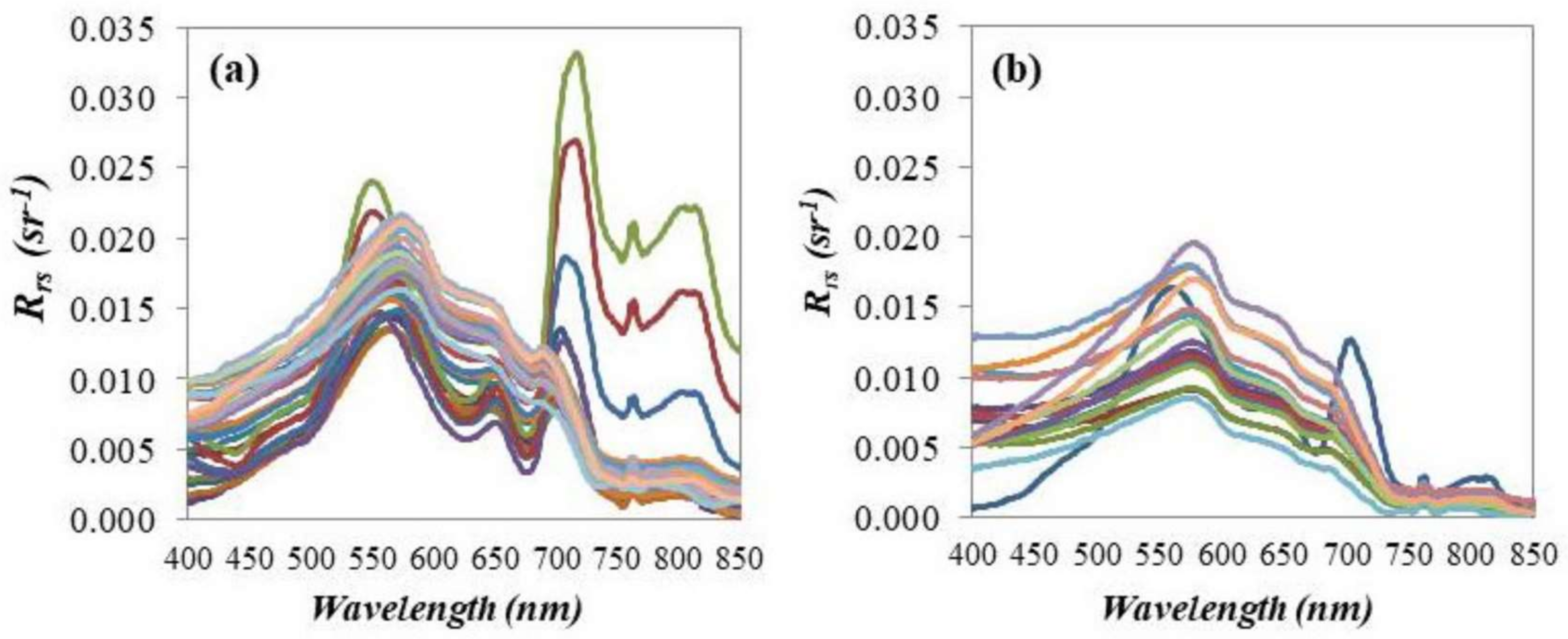
3.1. Remote Sensing Reflectance Spectra

In BAR1 spectral curves (Figure 2a) include a high absorption feature at about 680 nm, and a reflectance peak at approximately 710 nm that can be associated with the Chl-a pigment. The sampling sites with the highest Chl-a concentrations presented a significant peak at 550 nm, expected for water with a great amount of algae, as seen in the field. The increase of reflectance in longer wavelengths is indicative of the increase of the total suspended matter concentration. The Chl-a concentration in BAR1 was approximately 37 times higher than in BAR2 dataset (see

Table 2. Descriptive statistics for optical and water quality parameters for BAR1, BAR2, and the mixed data.

Field Campaigns	Parameters	Minimum	Maximum	Mean	S.D.	C.V.
BAR1 (N = 30)	ZSD (m)	0.5	1.6	1.2	0.2	20.0%
	Turbidity (NTU)	7.8	80.9	16.6	7.6	45.8%
	pH	6.1	9.9	7.9	0.8	10.5%
	Wind Speed (m s−1)	0.0	8.0	3.5	1.8	51.7%
	Depth (m)	5.6	19.6	11.4	4.3	37.8%
	kd(482) (m−1)	1.9	4.0	2.8	0.3	10.7%
	[Chl-a] (μg L−1)	25.7	709.9	119.8	96.4	80.5%
	[SPM] (mg L−1)	3.6	40.3	8.4	4.6	55.2%
	[IPM] (mg L−1)	0.9	4.0	2.3	0.5	21.9%
	[OPM] (mg L−1)	1.4	36.3	6.1	4.6	75.4%
	aϕ(482) (m−1)	0.2	4.2	0.4	0.3	68.0%
	aNAP(482) (m−1)	0.2	0.5	0.4	0.1	27.0%
	aCDOM(482) (m−1)	0.6	1.6	1.0	0.3	28.0%
BAR2 (N = 18)	ZSD (m)	1.6	2.5	2.1	0.2	9.3%
	Turbidity (NTU)	3.5	8.80	5.7	1.2	21.9%
	pH	6.8	7.3	7.0	0.1	1.9%
	Wind Speed (m s−1)	0.0	6.5	3.1	1.7	56.3%
	Depth (m)	4.7	21.2	12.7	4.1	32.6%
	kd(482) (m−1)	1.5	2.3	1.8	0.1	6.5%
	[Chl-a] (μg L−1)	3.8	19.1	8.0	3.3	40.9%
	[SPM] (mg L−1)	0.2	2.6	1.6	0.4	27.9%
	[IPM] (mg L−1)	0.2	1.3	0.6	0.2	42.4%
	[OPM] (mg L−1)	0.4	1.6	1.1	0.3	28.8%
	aϕ(482) (m−1)	0.02	0.1	0.1	0.02	33.0%
	aNAP(482) (m−1)	0.07	0.2	0.1	0.04	30.0%
	aCDOM(482) (m−1)	0.2	1.9	1.0	0.5	51.0%
Mixed Data (N = 48)	ZSD (m)	0.5	2.5	1.5	0.4	29.03%
	Turbidity (NTU)	3.5	80.9	12.7	6.3	50.03%
	pH	6.1	9.9	7.6	0.7	9.4%
	Wind Speed (m s−1)	0.0	8.0	3.3	1.8	53.4%
	Depth (m)	4.7	21.2	12.0	4.2	35.1%
	kd(482) (m−1)	1.5	4.0	2.4	0.5	21.1%
	[Chl-a] (μg L−1)	3.8	709.9	77.8	77.1	99.1%
	[SPM] (mg L−1)	0.2	40.3	5.8	4.05	69.8%
	[IPM] (mg L−1)	0.2	4.0	2.0	0.8	40.2%
	[OPM] (mg L−1)	0.4	36.3	5.0	4.0	79.5%
	aϕ(482) (m−1)	0.02	1.3	0.3	0.3	97.0%
	aNAP(482) (m−1)	0.07	0.5	0.3	0.1	53.0%
	aCDOM(482) (m−1)	0.2	1.9	1.0	0.4	37.0%

S.D. = Standard Deviation. C.V. = coefficient of variation.

), which explains why pigment absorption was more evident during the first survey. Still, in BAR1, the green and dark red curves (Figure 2a) represent two sampling points with expressive reflectance peaks at 550 nm and 700 nm and the highest values of Chl-a concentration of 709.89 μg L⁻¹ and 623.70 μg L⁻¹, respectively, among the other sampling points. Due to this high concentration of Chl-a some spectra presented the red edge feature as found in healthy vegetation, which explain the rise in the reflectance near 689 nm.

In both datasets, the organic particles were predominant (Table 2), therefore, the spectra of BAR1 and BAR2 were quite similar with less reflectance in BAR2 mainly because the lowest OSS concentrations were verified in relation to BAR1. In the BAR2 spectra, the features characteristic of phytoplankton absorption were not evident such as that for BAR1 due to the decrease of Chl-a concentration, with the exception of the feature of the sampling point that presented the maximum value of 19.11 μg L⁻¹ of the Chl-a concentration in BAR2 (navy blue curve in Figure 2b).

Light absorption by CDOM was highest in both field campaigns (1.57 $\pm$ 0.37 m⁻¹ in BAR1 and 1.98 $\pm$0.76 m⁻¹ in BAR2) in relation to light absorption by other OSSs. In CDOM-rich lakes, the spectra shapes vary according to CDOM levels and the influence of other substances in absorption processes [35]. In BAR1, the light absorption was dominated by CDOM, however, the reflectance spectra assumed a shape of Chl-a due to the high concentrations verified, and presented low reflectance values at 400–500 nm. In BAR2, with the predominance of CDOM in the light absorption process and the reduction of OSS concentrations, reflectance values assumed the nearly flat feature at ~600 nm.

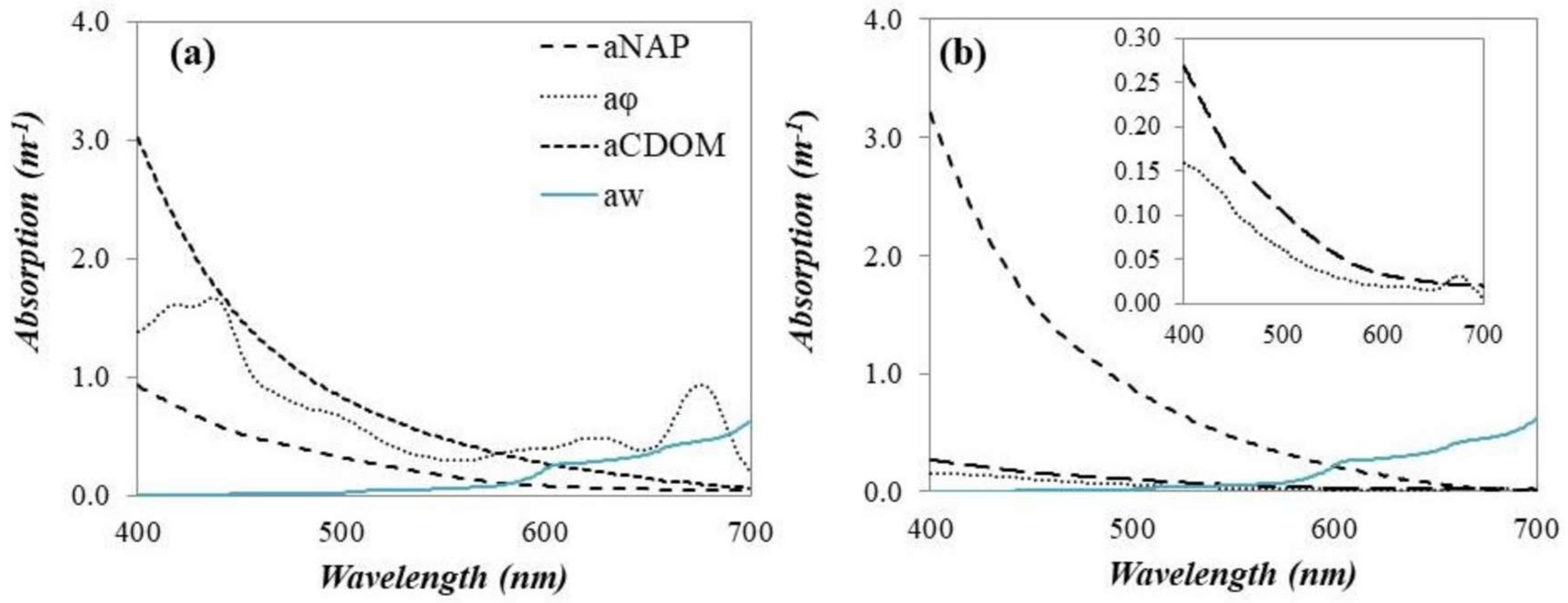
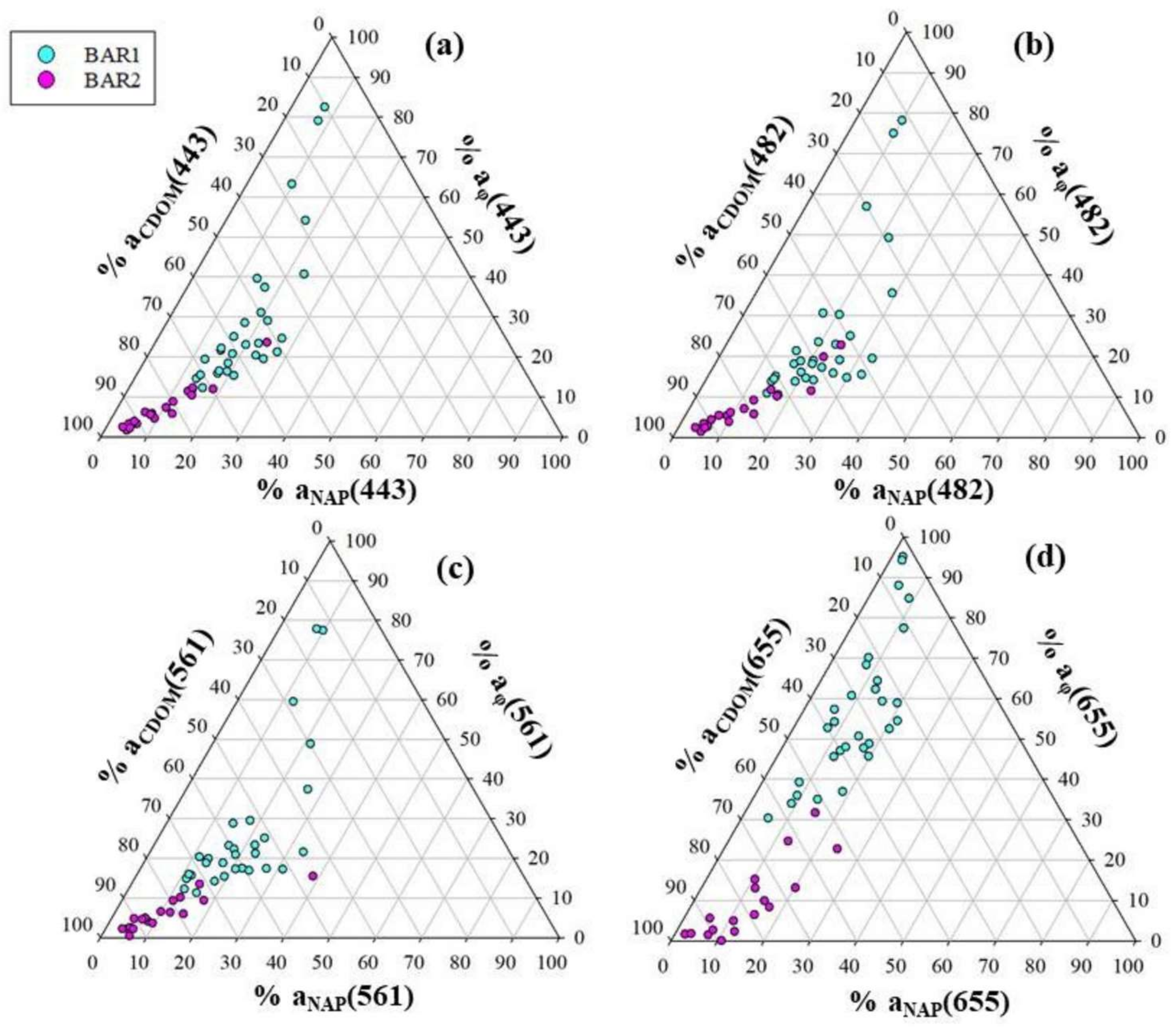
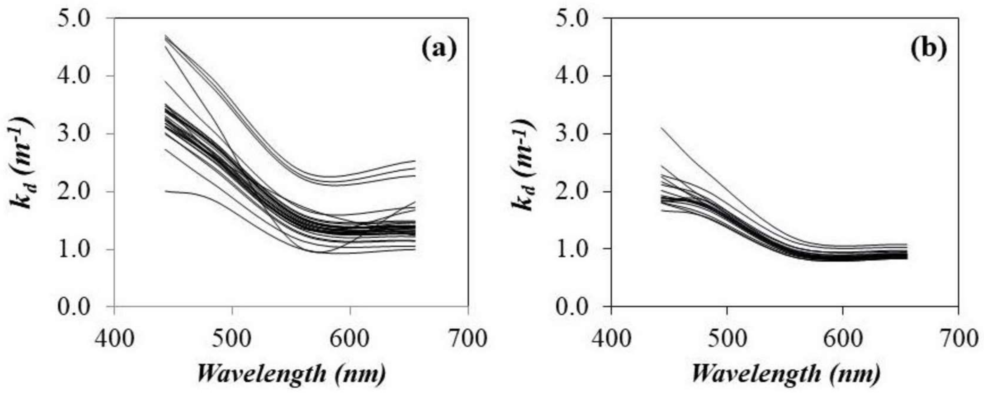
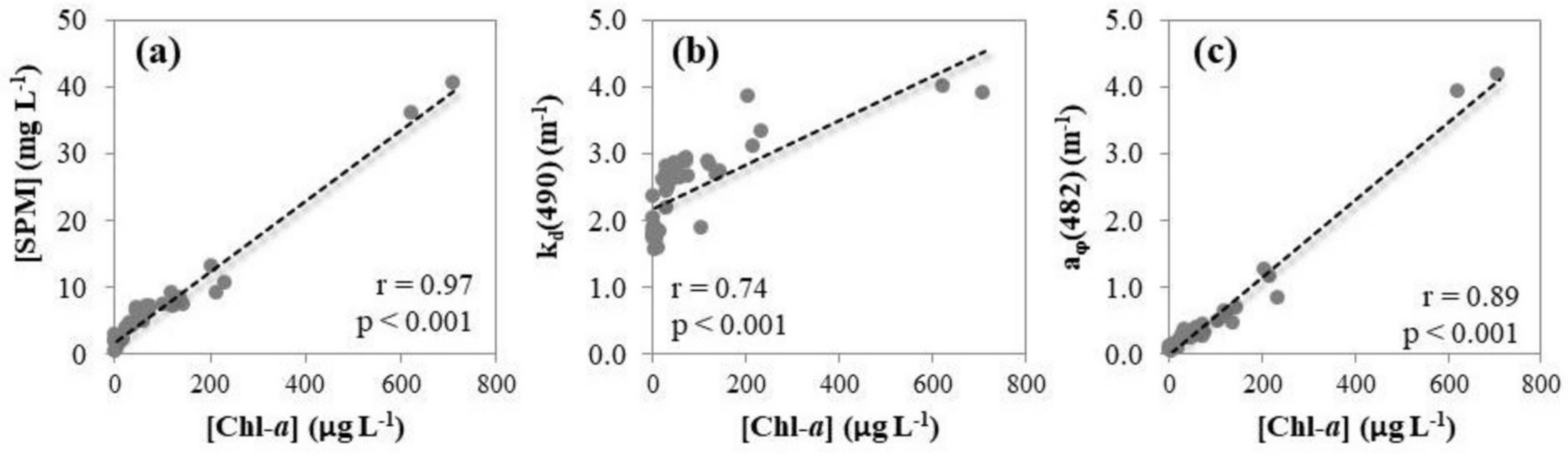
3.2. Optical Properties and Water Constituents

Table 2 presents the descriptive statistics for optical and water parameters for the two field campaigns, BAR1 and BAR2.

In BAR1, it was sunny with some overcast moments. In BAR2, the sky was more favorable with sunny days during all field campaigns. In all datasets, the average wind speed was 3.3 $\pm$ 1.8 m s⁻¹ producing some small waves on the water surface. The minimum values for both field campaigns were 0 m s⁻¹ and the maximum value was 8 m s⁻¹ in BAR1 and 6.5 m s⁻¹ in BAR2.

The water collected in BAR1 was green in most of the samples, which is explained by the presence of phytoplankton pigments due to high Chl-a concentration averaging 119.8 ± 96.4 μg L⁻¹, and ranging between 25.7 and 709.9 μg L⁻¹. In BAR2, the Chl-a variability reduced significantly, with an average of 8.0 $\pm$ 3.3 μg L⁻¹, varying from 3.8 to 19.1 μg L⁻¹. Therefore, the mixed data resulted in a range from 3.8 to 709.9 μg L⁻¹ of Chl-a.

The SPM concentration (average of 8.4 $\pm$ 4.6 mg L⁻¹) was predominately of organic particles with an average of 6.06 $\pm$ 4.57 mg L⁻¹ in BAR1, as well as in BAR2, corresponding to a major part of SPM (1.59 $\pm$ 0.44 mg L⁻¹) with an average of 1.11 $\pm$ 0.32 mg L⁻¹. The SPM presented a low concentration in BAR2. With respect to absorption, a_NAP(482) was higher in BAR1 (average of 0.4 $\pm$ 0.1 m⁻¹) than BAR2 (average of 0.1 $\pm$ 0.04 m⁻¹). The mean of a_CDOM(482) was 1.00 $\pm$ 0.3 m⁻¹ in BAR1 and 1.1 $\pm$ 0.6 m⁻¹ in BAR2. The mean of a_φ(482) was 0.7 $\pm$ 1.0 m⁻¹ in BAR1 and 0.07 $\pm$ 0.02 m⁻¹ in BAR2.

Figure 3 shows the average spectra of IOPs for BAR1 and BAR2 datasets. The a_φ spectra was higher in BAR1 than BAR2; it is possible to see two peaks of absorption at 450 and 670 nm in BAR1 (Figure 3a) whereas in BAR2 (Figure 3b) the characteristic a_φ spectra was not evident. In BAR2, the OSS concentration was less than in BAR1, therefore, the absorption processes were reduced in relation to BAR1, with the exception of a_CDOM. In BAR2, the a_φ and a_NAP spectra were similar with light absorption by NAP slightly higher than the absorption by phytoplankton, with the absorption curve decay at 550 nm (Figure 3b). The absorption curve of NAP in the blue portion of the visible spectrum represents the typical spectra of mineral and/or detrital particles, verified in BAR1 and BAR2 absorption spectra. The atypical a_φ spectra in BAR2, with the linear increase at wavelengths shorter than 500 nm, indicate an environment with elevated CDOM absorption [36].

Among the three absorption coefficients previously mentioned, a_CDOM(482) showed the highest values in both field campaigns. Zhang et al. [37] proved that high Chl-a concentration and high a_CDOM indicate that the accumulation and degradation of phytoplankton are a source of CDOM in eutrophic waters. Organic matter likely originates from phytoplankton degradation in BAR1. In BAR2, the a_CDOM is also predominant with significant reduction of Chl-a concentration, which can suggest an allochthonous source of CDOM. The Bariri reservoir has been experiencing impacts due to sugarcane production and the input of urban and industrial wastewaters [38,39]. The proportional contribution of the IOPs in BAR1 and BAR2 among the total absorption (a_t) budget in the Bariri aquatic environment was computed considering the OLI bands (443, 482, 561, and 655 nm) (Figure 4a–d).

Absorption in BAR1 was predominant by CDOM at 443, 482, and 561 nm, with 53.6 $\pm$ 16.4%; 54.7 $\pm$ 16% and 55.7 $\pm$ 16.6%, respectively. At 655 nm, the phytoplankton contribution was the highest with 56.7 $\pm$ 17.6%. The same was verified for BAR2, where the CDOM predominance was even higher, with 82.7 $\pm$ 10.6% at 443 nm; 80.8 $\pm$ 12.3% at 482 nm; and 78.3 $\pm$ 13.5% at 655 nm; but with the highest contribution at 561 nm with 83.1 $\pm$ 11.6%.

In BAR1, the phytoplankton contributed 28.8 $\pm$ 18.4%, 25 $\pm$ 17.5%, 26.1 $\pm$ 17.4%, and 56.7 $\pm$ 17.6% at 443, 482, 561, and 655 nm, respectively. The highest proportions at the blue and red spectral regions confirm the absorption peaks by Chl-a pigment. In sequence, the NAP presented the lowest proportion of the absorption budget with 17.6 $\pm$ 5.1% at 443 nm; 20.3% $\pm$ 6.1% at 482 nm; 18.2 $\pm$ 6.4% at 561 nm, and 11.7 $\pm$ 5.4% at 655 nm. The peak of NAP absorption in the blue spectral region is typical of detrital or mineral particles, which were also verified in BAR2, with 10 $\pm$ 5.4% and 11.6 $\pm$ 6.7% at 443 and 482 nm, respectively, and 10.8 $\pm$ 8% at 561 nm and 11.9 $\pm$ 5.6% at 655 nm. The phytoplankton achieved 7.3 $\pm$ 5.3% at 443 nm, 7.6 $\pm$ 5.9% at 482 nm, and 9.8 $\pm$ 9.3% at 655 nm, being higher in the blue and red spectral regions, respectively. At 561 nm, the percentage was 6.1 $\pm$ 4.1%. Considering both datasets, the Chl-a concentration had an average of 77.8 $\pm$ 77.1 μg L⁻¹ and the organic particles had the highest concentration (5.0 $\pm$ 4.0 mg L⁻¹), with the greater part of light absorbed by CDOM.

The average of k_d(490) in BAR1 and BAR2 was 2.8 $\pm$ 0.3 m⁻¹ (ranging from 1.9 to 4.0 m⁻¹) and 1.8 $\pm$ 0.1 m⁻¹ (ranging from 1.5 to 2.3 m⁻¹), respectively. The water column was more attenuated in August 2016 than June 2017. Both months are in the dry season; however, 2016 presented the highest mean rate of precipitation from January to June when compared with 2017 over the Bariri reservoir area (Figure 1d). The rain carries organic matter, mainly from industrial effluents, wastewater, and particulate matter to the Bariri reservoir, as well as facilitates the increase of organic matter fluxes along the Tietê River from upstream to downstream. The Tietê River is in one of the most industrialized basins of São Paulo State and the reservoir’s construction promoted the rapid transformation in the land use and land cover, facilitating the pollution problems and accelerating the sedimentation process [38]. The concentration of water constituents was higher in August, increasing the process of absorption and the backscattering of light and, consequently, showing the highest k_d(490) values. Figure 5 presents the spectra of k_d derivation of BAR1 and BAR2.

After normalization of Ed measurements, it was possible to derive k_d in an accurate way and reduce the noise introduced by the wave-focusing. In BAR1, the k_d(490) showed higher magnitude in relation to BAR2.

In both field surveys, the SPM concentration ([SPM]) was dominated by organic matter. The relationship between [SPM] and Chl-a concentration ([Chl-a]) presented a significant positive correlation (R = 0.97; p < 0.001) for the mixed data (Figure 6a). High proportions of [Chl-a] in water indicate excessive input of nutrients which increase the attenuation of light in water [39], verified by the positive correlation (R = 0.74; p < 0.001) between k_d(490) and [Chl-a] for the Bariri mixed data (Figure 6b). The nutrient enrichment in water accelerated the primary productivity with a great amount of phytoplankton production, confirmed by the strong relationship between [Chl-a] and a_ϕ(482) (R = 0.89; p < 0.001) in Figure 6c.

3.3. Assessment of the Vertical Attenuation Coefficient Models

Due to a lack of data from turbid inland waters used in the calibration of k_d(490) algorithms, the application for the Bariri reservoir can be compromised. The algorithm coefficients developed for a wide range of waters tried to minimize this limitation although it is not a guarantee of success [25]. For all k_d(490) algorithms, bands were defined according to the center bands from OLI/Landsat-8, including the blue band at 490 nm that was replaced by 482 nm.

Table 3. Error assessment of k_d(490) models developed for clear, slightly turbid, turbid ocean waters, coastal waters and global waters applied to all dataset of Bariri.

Type	Model	MAPE (%)	RMSE (m−1)	bias (m−1)
Empirical	Morel et al. (2007) I	61.0	1.5	−1.2
	Morel et al. (2007) II	61.0	1.5	−1.2
	Mueller (2000)	86.5	2.2	−2.1
	Mueller and Tress (1997)	86.1	2.2	−2.1
	Chauhan et al. (2003)	82.3	2.0	−1.9
	Werdell (2005)	86.0	2.2	−2.1
	Kratzer et al. (2008)	60.6	1.6	−1.5
	Zhang and Fell (2007)	42.9	1.2	−2.0
	Wang et al. (2009)	54.0	1.4	−1.1
Semi-analytical	Wang et al. (2009) I	46.3	1.3	−1.2
	Wang et al. (2009) II	63.7	1.7	−1.6
	Lee et al. (2013)	41.0	2.0	−0.9

summarized the statistical results yielded after the application of k_d(490) models.

The empirical models of k_d(490) based on Chl-a concentration underestimated the results for almost the entire dataset, except for two samples with high values of Chl-a concentration which were overestimated. The coefficients of the model from Morel et al. [3] were developed for Case I waters, with the optical properties dominated by phytoplankton, therefore, the accuracy of the model in aquatic environments with high rates of CDOM and/or suspended solids is expected to fail [28]. The models from Morel et al. [3] were calibrated with open ocean waters with values of Chl-a < 2.4 μg L⁻¹, much lower of the values found in Bariri reservoir, resulting in k_d(490) errors of MAPE ~61% and RMSE ~1.5 m⁻¹.

The empirical models using the nL_w spectral ratio developed for ocean open and global waters presented the worst results with MAPE around 80% and RMSE ~2 m⁻¹. Mueller [5], Mueller and Tress [6], Chauhan et al. [7], and Werdell [40] models underestimated the results of k_d(490) with bias around 2 m⁻¹. The calibration dataset involved waters with values of k_d(490) up to 0.6 m⁻¹ whereas, in Bariri, all datasets varied from 1.5 to 4.0 m⁻¹.

The blue-green ratio nL_w(490)/nL_w(555) or R_rs(490)/R_rs(555) have large uncertainties when k_d(490) is greater than 0.2 m⁻¹. The spectral ratio presents an asymptotic value with increasing OSS concentration [5]. Thus, this spectral ratio is not sensitive for the variations in OSS that occurred in turbid inland waters, resulting in significant underestimation of k_d(490). In addition, this spectral ratio does not consider the effects of solar angle changes that decrease the accuracy of empirical algorithms for estimating k_d(490) [25].

Aiming to investigate the estimation of k_d(490) from MERIS, Kratzer et al. [8] developed the empirical algorithm using the ratio of 490 nm and 620 nm for Case 2 water optically dominated by CDOM, which showed an inverse relationship to salinity in the Baltic Sea. The Kratzer et al. [8] model applied to all datasets from Bariri presented a MAPE of 60.6% and an RMSE of 1.6 m⁻¹.

The empirical algorithm developed by Wang et al. [9] combined open ocean and turbid coastal waters (from 0.3 to 0.6 m⁻¹) through a linear regression equation of the R_rs(670)/R_rs(490) ratio that showed better matching of k_d(490) data when the k_d(490) values of calibrated data were higher than 0.3 m⁻¹. The application of this model in the Bariri reservoir data resulted in a MAPE of 54.0% and an RMSE of 1.4 m⁻¹, yielding underestimated values (bias of −1.1) of k_d(490).

The semi-analytical algorithms of Wang et al. [9] were developed considering the MODIS satellite data and the absorption and backscattering coefficients derived from Lee et al. [11]. The algorithm based on the ratio R(667)/R(488) presented a MAPE of 46.3% and an RSME of 1.3 m⁻¹, while the ratio R(645)/R(488) showed a MAPE around 63.7% and an RMSE of 1.7 m⁻¹. The OLI sensor does not have a spectral band centered at 488, neither at 667 nm, nor at 645 nm, but at 482 and 655 nm, respectively. Therefore, in both semi-analytical equations, R(482) and R(655) were used and the differences found in the results above are explained by the coefficients, which, in the first model, presented better adjustment than the second model in the Bariri reservoir.

The Zhang and Fell [29] empirical algorithm and the semi-analytical algorithm developed by Lee et al. [10] presented similar performances corresponding to a MAPE of 42.90%, an RMSE of 1.22 m⁻¹, and a MAPE of 41.0%, and an RMSE of 1.1 m⁻¹, respectively. Calibrated with a wide range of environments (0.01–4.6 m⁻¹), the Zhang and Fell [29] model have showed greater correlation for clear waters, whereas the Lee et al. [10] algorithm showed the greatest application for turbid waters, such as what occurs in this study site. The difference in errors among these empirical and semi-analytical algorithms could be explained by the use of the 655 nm wavelength in the Zhang and Fell [29] model, which introduces noise due to the high absorption rate of water in the red wavelength, even after corrections in data processing.

The Lee et al. [10] semi-analytical algorithm showed the lowest errors (MAPE = 41.0%; RMSE = 1.1 m⁻¹) for k_d(490) estimate in the Bariri reservoir. In inland waters, the regional variability of the OSSs generate significant changes in the attenuation of the light process, therefore, the Lee et al. [10] algorithm in considering a(λ) and b_b(λ), estimated via QAA_v5 [31], and the sun angle resulted in fewer uncertainties regarding data matching. Additionally, the algorithms’ coefficients derived from numerical simulations reduce the dependence of a specific data range.

Empirical algorithms were developed (results not shown here) from Bariri using all datasets, however, the results were not satisfactory. Therefore, the Lee et al. [10] model was chosen for mapping the variability of k_d(490) in the study site.

3.4. Assessment of the OLI Atmospheric Correction Product

The evaluation of LaSRC accuracy consisted in the comparison between the OLI-derived R_rs product from August 2016 and the R_rs calculated from TriOS data in BAR1. The relative percentage errors were 50.1% at 443 nm, 20.7% at 482 nm, 17.2% at 561 nm, and 29.6% at 655 nm. The highest errors in the coastal and blue regions are related to the increase of scattering in those regions. The lowest error is verified in the green region with 17.2% and, in sequence, in the red region, the error increased again to 29.6%. The LaSRC accuracy results encountered here are compatible with the atmospheric correction analysis presented in Rodrigues, T. et al. [41] and Bernardo, N. et al. [33].

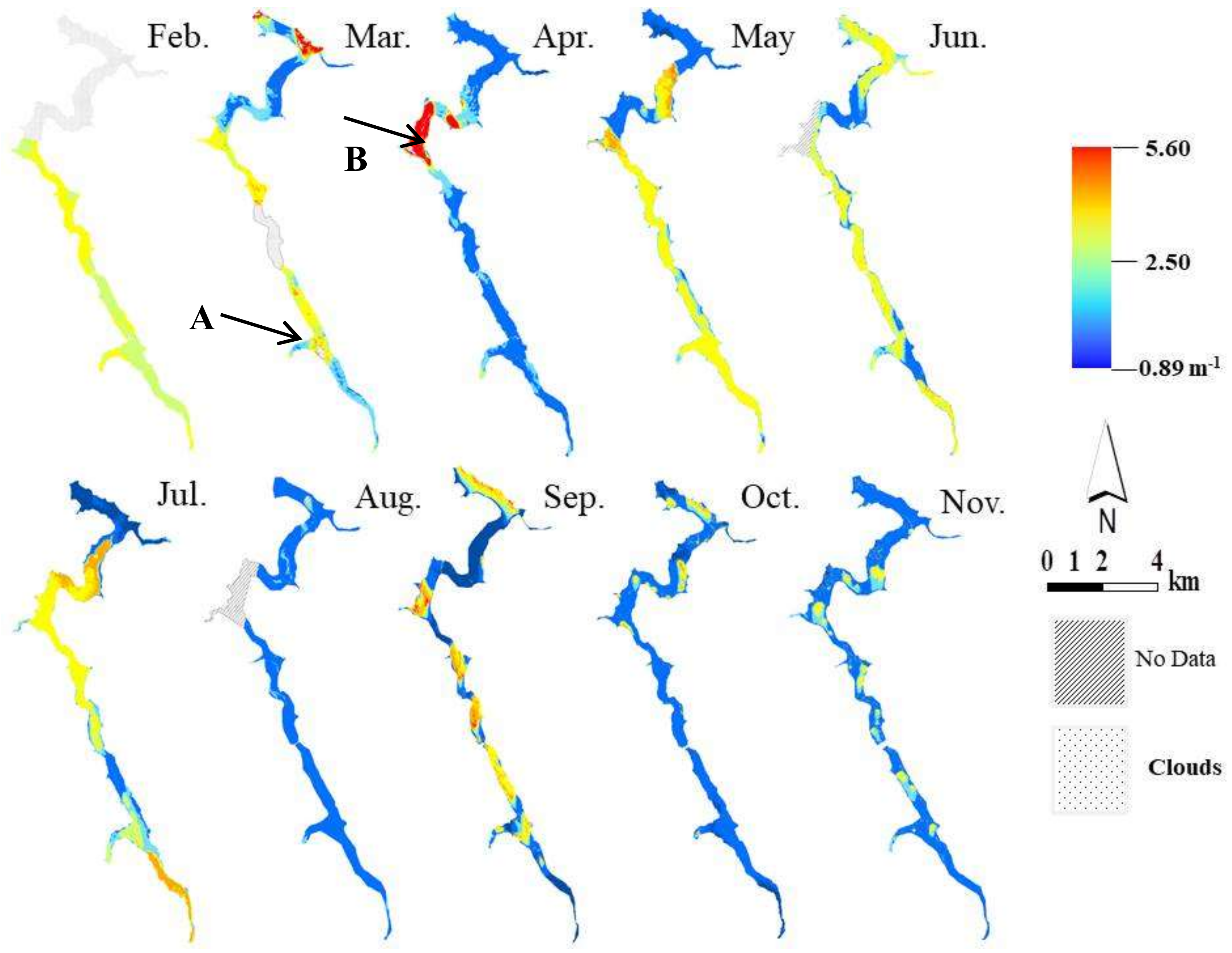
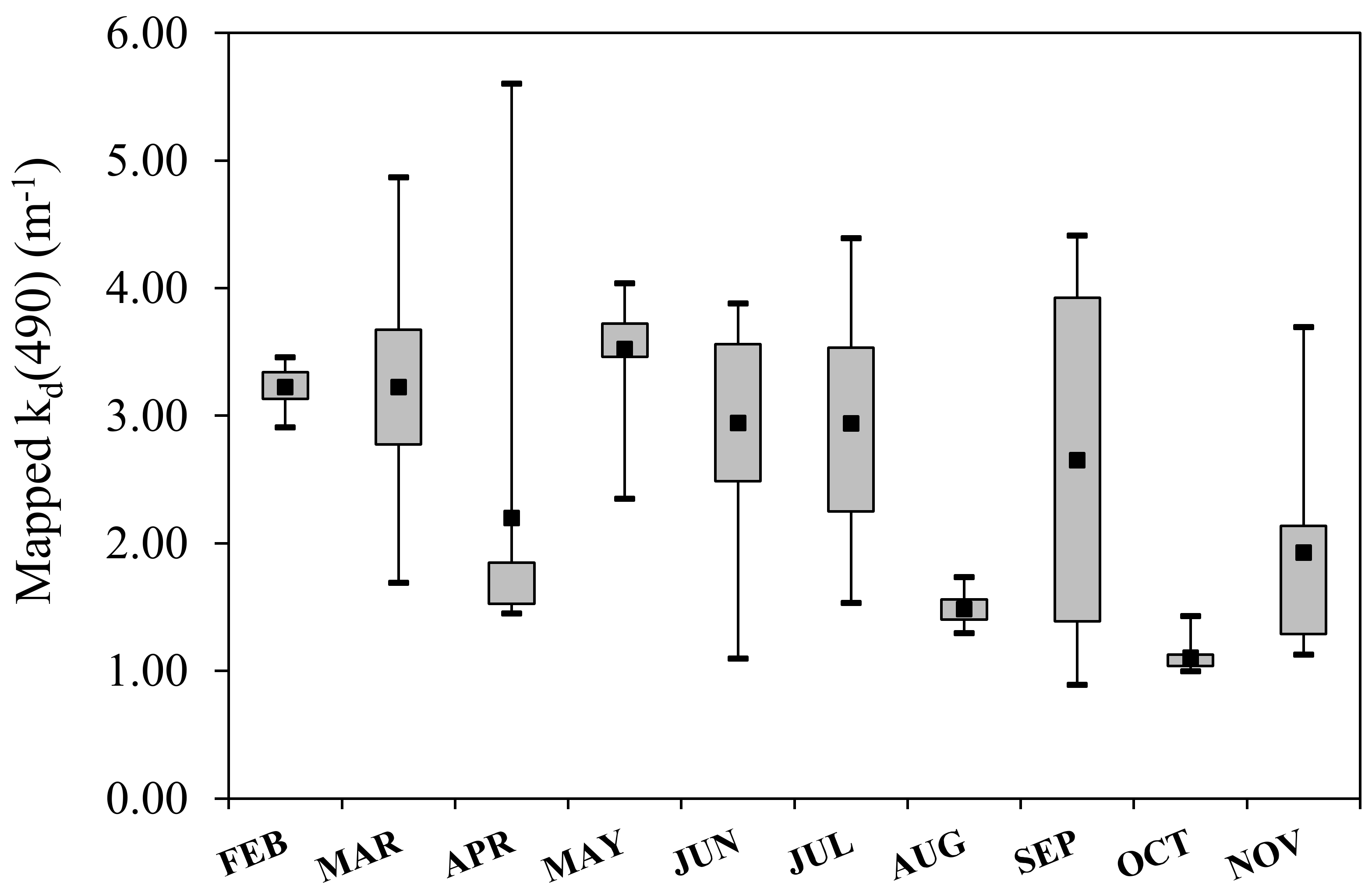
3.5. Application of k_d(490) on OLI/Landsat-8 Images

The variability of k_d(490) in the Bariri reservoir expressed in OLI/Landsat-8 is presented in Figure 6. The spatial distribution of Lee et al. [10] in the Bariri reservoir was validated from the k_d(490) estimates obtained from the image of 15 August and presented a MAPE of 32.5% and an RMSE of 0.9 m⁻¹. The errors of k_d(490) estimates from the Lee et al. [10] model, applied for all datasets, using the in situ R_rs, were 41.0% of MAPE and 1.1 m⁻¹ of RMSE. The differences between the k_d(490) estimations from in situ R_rs and R_rs from LaSRC are related to the decrease of the variability among the sampling points through the sample size reduction that, in the former case, was 48 (all datasets) and, in the latter case, was 26 (four sampling points with missing information in the image from August in the region highlighted as zone B in Figure 7) that presented the lowest errors.

The increase of the percentage error between the OLI-derived R_rs at 482 nm used as the input of k_d(490) estimation and the k_d(490) estimations for BAR1 was 11.9% and could be related to IOP estimations via QAA_v5. The application with no modifications in some empirical steps can affect the QAA_v5 performance in optically-complex waters [42,43].

The maximum value of k_d(490) was 5.60 m⁻¹ in April and the minimum value was 0.89 m⁻¹ in September, both in the dry season. In the image from April, specifically in zone B highlighted by the arrow, an expressive increase of the k_d(490) was observed, which is probably related to the reduction of water velocity favoring the increase of Chl-a concentration and, in a dramatic way, an algal bloom, intensifying the attenuation of light in the water. The decomposition of algae within the water can characterize a source of CDOM, which also intensifies the attenuation of light in the water [35]. Along the reservoir, except for zone B, the k_d(490) values remained below the mean (Figure 7), which was expected for a period of low precipitation, confirming an atypical event in April. In September, the k_d(490) was uniformly distributed around the mean, with values closer to the maximum (4.40 m⁻¹) in the northeast region of the reservoir which presents agricultural activities and bare soil areas that facilitates the input of external material into the reservoir even in periods of low precipitation. Other regions with high values of k_d(490) were in zone B and another bend where water flux is slower than in zone A.

The boxplot in Figure 8 summarizes the variability of k_d(490) for each month. In the dry season, the k_d(490) values were closer to the maximum in May and June, with most values above the mean and, concomitantly, values above 2.5 m⁻¹ in zone A. In July and August, the k_d(490) started to decrease with most of the values closer to the minimum and below the mean, with a decrease of k_d(490) in zone A. The precipitation rates were quite smaller in July (~4.0 mm) and August (~53.8 mm) than in May (~125.2 mm) and June (~125.4 mm), in conjunction with a reduction of k_d(490) in zone A, which could be revealed as a point source of wastewater.

Unfortunately, the image from August, coincident with the BAR1 field campaign, has no information in the region highlighted as zone B that prevents showing the highest Chl-a concentrations in these sampling points, which generated high values of k_d(490) as mentioned in Section 3.1. The mean was 1.5 m⁻¹, with values closer to the minimum, ranging from 1.3 to 1.7 m⁻¹, not corresponding with in situ k_d(490). The precipitation rate in August was very low, resulting in a low k_d(490) in zone A. The months of October, November, February, and March are representative of the wet season, however, in October, the mean k_d(490) almost coincided with the minimum resulting in low values with some peaks northeast of the reservoir and in a winding region.

In November, the increase of k_d(490) was observed with the mean closer to the maximum value, presenting some points above 2.5 m⁻¹. In February, with higher precipitation rates than the months previously mentioned, the k_d(490) was around 3.0 m⁻¹ even with approximately 30% of the reservoir covered by clouds. In March, the k_d(490) was well distributed around the mean, ranging from 1.7 to 4.9 m⁻¹, with the highest values in the northeast and extremely north of the reservoir and values above 2.5 m⁻¹ in some parts of zone B and in zone A.

4. Conclusions

After the application of several tests to estimate k_d(490) through the available models developed to a wide range of waters, it was verified that empirical models do not estimate the k_d(490) accurately in the Bariri reservoir. The uncertainty presented by the empirical models (~80% of MAPE) confirms that the blue/green wavelength ratio is not able to express the k_d(490) variability in an environment dominated by CDOM, which was verified in the two surveys. The empirical models with Chl-a concentration as the input presented intermediary errors (~60% of MAPE) when applied to the aggregated data from the two surveys realized. In BAR1, the Chl-a concentration was significantly higher than in BAR2; the light absorption by CDOM was maintained predominantly in both surveys. Among the tested empirical models, the model developed by Zhang and Fell [29] was an exception in achieving lower errors and statistical results close to those obtained from the semi-analytical models.

The semi-analytical model developed by Lee et al. [9] presented the lowest error (MAPE of 41.0%) among all twelve models analyzed. The coefficients present in the Lee et al. [9] model were calibrated from a wide range of waters, filling the lack of the empirical models that are based on a specific dataset. However, the IOPs’ estimates through the original QAA_v5 can introduce some errors in inland waters due to the optical complexity.

The Lee et al. [9] model was applied in atmospherically-corrected OLI/Landsat-8 images (LaSRC) with a relative error percentage difference of 8.5% in relation to the application to all datasets from the R_rs obtained in situ. Therefore, the atmospheric correction was appropriate to retrieve the k_d(490) and the Lee et al. [9] model was able to highlight the main variations of k_d(490) in an environment dominated by CDOM in the Bariri reservoir, allowing the identification of the regions with more or less light attenuation and, consequently, the biota modifications that are dependent of the photic conditions in the water column.

The application of the k_d(490) model on OLI/Landsat-8 images exhibited important temporal and spatial variability. The spatial variability was verified in points where the sinuosity of the reservoir promoted the reduction of water velocity and facilitated the OSS concentrations, increasing the attenuation of light. The temporal variability was linked to significant activities around the reservoir that increase the runoff and the input of external material into the reservoir mainly in periods of high precipitation rates. Additionally, the precipitation in the wet season promotes the resuspension and carriage of sediments, increasing the attenuation of light.

References

1. Mobley, C.D. Light and Water: Radiative Transfer in Natural Waters; Academic Press: San Diego, CA, USA, 1994. [Google Scholar]
2. Zheng, Z.; Ren, J.; Li, Y.; Huang, C.; Liu, G.; Du, C.; Lyu, H. Remote sensing of diffuse attenuation coefficient patterns from Landsat 8 OLI imagery of turbid inland waters: A case study of Dongting Lake. Sci. Total Environ. 2016, 573, 39–54. [Google Scholar] [CrossRef] [PubMed]
3. Morel, A.; Huot, Y.; Gentili, B.; Werdell, P.J.; Hooker, S.B.; Franz, B.A. Examining the consistency of products derived from various ocean color sensors in open ocean (Case 1) waters in the perspective of a multi-sensor approach. Remote Sens. Environ. 2007, 111, 69–88. [Google Scholar] [CrossRef]
4. Zhang, Y.; Liu, X.; Yin, Y.; Wang, M.; Qin, B. A simple optical model to estimate diffuse attenuation coefficient of photosynthetically active radiation in an extremely turbid lake from surface reflectance. Opt. Express 2012, 20, 482–493. [Google Scholar] [CrossRef] [PubMed]
5. Mueller, J.L. SeaWiFS algorithm for the diffuse attenuation coefficient, Kd(490) using water-leaving radiance at 490 and 555 nm. SeaWiFS Post Launch Tech. Rep. Ser. 2000, 11, 24–27. [Google Scholar]
6. Mueller, J.L. Revised SeaWiFS Prelaunch Algorithm for Diffuse Attenuation Coefficient K(490); Trees, C.C., Ed.; NASA Goddard Space Flight Center: Greenbelt, MD, USA, 1997. [Google Scholar]
7. Chauhan, P.; Sahay, A.; Rajawat, A.S.; Nayak, S. Remote sensing of diffuse attenuation coefficient (K490) using IRS-P4 Ocean Colour Monitor (OCM) sensor. Indian J. Mar. Sci. 2003, 32, 279–284. [Google Scholar]
8. Kratzer, S.; Brockmann, C.; Moore, G. Using MERIS full resolution data to monitor coastal waters—A case study from Himmerfjärden, a fjord-like bay in the northwertern Baltic Sea. Remote Sens. Environ. 2008, 112, 2284–2300. [Google Scholar] [CrossRef]
9. Wang, M.; Son, S.; Harding, L.W., Jr. Retrieval of diffuse attenuation coefficient in the Chesapeake Bay and turbid ocean regions for satellite ocean color applications. J. Geophys. Res. 2009, 114, 1–15. [Google Scholar] [CrossRef]
10. Lee, Z.P.; Hu, C.; Shang, S.; Du, K.; Lewis, M.; Arnone, R.; Brewin, R. Penetration of UV-visible solar radiation in the global oceans: Insights from ocean color remote sensing. J. Geophys. Res. Oceans 2013, 118, 4241–4255. [Google Scholar] [CrossRef] [Green Version]
11. Lee, Z.P.; Carder, K.L.; Arnone, R.A. Deriving inherent optical properties from water color: A multiband quasi-analytical algorithm for optically deep waters. Appl. Opt. 2002, 41, 5755–5772. [Google Scholar] [CrossRef] [PubMed]
12. Gallegos, C.L.; Correll, D.L.; Pierce, J.W. Modeling spectral diffuse attenuation, absorption, and scattering coefficients in a turbid estuary. Limnol. Oceanogr. 1990, 35, 1486–1502. [Google Scholar] [CrossRef]
13. Tundisi, J.G.; Matsumura-Tundisi, T.; Pareschi, D.C.; Luzia, A.P.; Von Haeling, P.H.; Frollini, E.H. A bacia hidrográfica do Tietê/Jacaré: Estudo de caso em pesquisa e gerenciamento. Estud. Av. 2008, 22, 159–172. [Google Scholar] [CrossRef]
14. Barbosa, F.A.R.; Padisák, J.; Espíndola, E.L.G.; Borics, G.; Rocha, O. The cascading reservoir continuum concept (CRCC) and its application to the river Tietê-basin, São Paulo State, Brazil. Theor. Reserv. Ecol. Its Appl. 1999, pp. 425–438. Available online: http://real.mtak.hu/3269/ (accessed on 20 June 2018).
15. Golterman, H.L.; Clymo, R.S.; Ohnstad, M.A.M. Methods for Physical and Chemical Analysis of Fresh Water; Blackwell Scientific: Oxford, UK, 1978; p. 214. [Google Scholar]
16. APHA. Standard Methods for the Examination of Water and Wastewater; American Public Health Association: Washington, DC, USA, 1998; p. 20. [Google Scholar]
17. Bricaud, A.; Morel, A.; Prieur, L. Absorption by dissolved organic matter of the sea (yellow substance) in the UV and visible domains. Limnol. Oceanogr. 1981, 26, 43–53. [Google Scholar] [CrossRef]
18. Tassan, S.; Ferrari, G.M. An alternative approach to absorption measurements of aquatic particles retained on filters. Limnol. Oceanogr. 1995, 40, 1358–1368. [Google Scholar] [CrossRef] [Green Version]
19. Tassan, S.; Ferrari, G.M. Measurement of light absorption by aquatic particles retained on filters: Determination of the optical path length amplification by the ‘transmittance-reflectance’ method. J. Plankton Res. 1998, 20, 1699–1709. [Google Scholar] [CrossRef]
20. Tassan, S.; Ferrari, G.M. A sensitivity analysis of the ‘Transmittance–Reflectance’ method for measuring light absorption by aquatic particles. J. Plankton Res. 2002, 24, 757–774. [Google Scholar] [CrossRef]
21. Mobley, C.D. Estimation of the remote-sensing reflectance from above-surface measurements. Appl. Opt. 1999, 38, 7442–7455. [Google Scholar] [CrossRef] [PubMed]
22. Lee, Z.P.; Ahn, Y.H.; Mobley, C.; Arnone, R. Removal of surface-reflected light for the measurement of remote-sensing reflectance from an above-surface platform. Opt. Express 2010, 18, 26313–26324. [Google Scholar] [CrossRef] [PubMed]
23. Barsi, J.A.; Lee, K.; Kvaran, G.; Markham, B.L.; Pedelty, J.A. The spectral response of the Landsat-8 Operational Land Imager. Remote Sens. 2014, 6, 10232–10251. [Google Scholar] [CrossRef]
24. Lee, Z.P.; Du, K.P.; Arnone, R. A model for the diffuse attenuation coefficient of downwelling irradiance. J. Geophys. Res. 2005, 110, 1–10. [Google Scholar] [CrossRef]
25. Gege, P.; Pinnel, N. Sources of variance of downwelling irradiance in water. Appl. Opt. 2011, 50, 2192–2203. [Google Scholar] [CrossRef] [PubMed]
26. Mishra, D.R.; Narumalani, S.; Rundquist, D.; Lawson, M. Characterizing the vertical diffuse attenuation coefficient for downwelling irradiance in coastal waters: Implications for water penetration by high resolution satellite data. Photogramm. Remote Sens. 2005, 60, 48–64. [Google Scholar] [CrossRef]
27. Kirk, J.T.O. Light & Photosynthesis in Aquatic Ecosystems, 2nd ed.; Cambridge University Press: Melbourne, Australia, 1994. [Google Scholar]
28. Zhao, J.; Barnes, B.; Melo, N.; English, D.; Lapointe, B.; Muller-Karger, F.; Schaeffer, B.; Hu, C. Assessment of satellite-derived diffuse attenuation coefficients and euphotic depths in south Florida coastal waters. Remote Sens. Environ. 2013, 131, 35–50. [Google Scholar] [CrossRef]
29. Zhang, T.; Fell, F. An empirical algorithm for determining the diffuse attenuation coefficient kd in clear and turbid waters from spectral remote sensing reflectance. Limnol. Oceanogr. Methods 2007, 5, 457–462. [Google Scholar] [CrossRef]
30. Lee, Z.P.; Lubac, B.; Werdell, J.; Arnone, R. An Update of the Quasi-analytical Algorithm (QAA_v5). In International Ocean Color Group Software Report; International Ocean-Colour Coordinating Group: Dartmouth, Nova Scotia, NS, Canada, 2009; pp. 1–9. [Google Scholar]
31. Vermote, E.; Justice, C.; Claverie, M.; Franch, B. Preliminary analysis of the performance of the Landsat 8/OLI land surface reflectance product. Remote Sens. Environ. 2016, 185, 46–56. [Google Scholar] [CrossRef]
32. Pahlevan, N.; Schott, J.R.; Franz, B.A.; Zibordi, G.; Markham, B.; Bailey, S.; Schaaf, C.B.; Ondrusek, M.; Greb, S.; Strait, C.M. Landsat 8 remote sensing reflectance (Rrs) products: Evaluations, intercomparisons, and enhancements. Remote Sens. Environ. 2017, 190, 289–301. [Google Scholar] [CrossRef]
33. Bernardo, N.; Watanabe, F.; Rodrigues, T.; Alcântara, E. Atmospheric correction issues for retrieving total suspended matter concentrations in inland waters using OLI/Landsat-8 image. Adv. Space Res. 2017, 59, 2335–2348. [Google Scholar] [CrossRef]
34. Moses, W.J.; Gitelson, A.A.; Perk, R.L.; Gurlin, D.; Rundquist, D.C.; Leavitt, B.C.; Barrow, T.M.; Brakhage, P. Estimation of chlorophyll-a in turbid productive waters using airborne hyperspectral data. Water Res. 2012, 46, 993–1004. [Google Scholar] [CrossRef] [PubMed]
35. Brezonik, P.L.; Olmanson, L.G.; Finlay, J.C.; Bauer, M.E. Factor affecting the measurement of CDOM by remote sensing of optically complex inland waters. Remote Sens. Environ. 2015, 157, 199–215. [Google Scholar] [CrossRef]
36. Binding, C.E.; Jerome, J.H.; Bukata, R.P.; Booty, W.G. Spectral absorption properties of dissolved and particulate matter in Lake Erie. Remote Sens. Environ. 2008, 112, 1702–1711. [Google Scholar] [CrossRef]
37. Zhang, Y.; van Dijk, M.A.; Liu, M.; Zhu, G.; Qin, B. The contribution of phytoplankton degradation to chromophoric dissolved organic matter (CDOM) in eutrophic shallow lakes: Field and experimental evidence. Water Res. 2009, 43, 4685–4697. [Google Scholar] [CrossRef] [PubMed]
38. Prado, R.B.; Novo, E.M.L.M.; Pereira, M.N. Evaluation of Land Use and Land Cover Dynamics in the Hydrographic Contribution Basin of Barra Bonita Reservoir-SP. Braz. J. Cartogr. 2007, 2, 127–135. [Google Scholar]
39. Cairo, C.T.; Barbosa, C.C.F.; Novo, E.M.L.M.; Calijuri, M.C. Spatial and seasonal variation in diffuse attenuation coefficients of downward irradiance at Ibitinga Reservoir, São Paulo, Brazil. Hydrobiologia 2017, 784, 265–282. [Google Scholar] [CrossRef]
40. Werdell, P.J. OceanColor K490 Algorithm Evaluation. Available online: https://oceancolor.gsfc.nasa.gov/reprocessing/r2005.1/seawifs/k490_update/ (accessed on 17 October 2017).
41. Rodrigues, T.; Alcântara, E.; Watanabe, F.; Imai, N. Retrieval of Secchi disk depth from a reservoir using a semi-analytical scheme. Remote Sens. Environ. 2017, 198, 213–228. [Google Scholar] [CrossRef]
42. Watanabe, F.; Mishra, D.R.; Astuti, I.; Rodrigues, T.; Alcântara, E.; Imai, N.N.; Barbosa, C. Parametrization and calibration of a quase-analytical algorithm for tropical eutrophic waters. ISPRS J. Photogramm. Remote Sens. 2016, 121, 28–47. [Google Scholar] [CrossRef]
43. Li, S.; Song, K.; Mu, G.; Zhao, Y.; Ma, J.; Ren, J. Evaluation of the Quasi-Analytical Algorithm (QAA) for estimating total absorption coefficient of turbid inland Waters in Northeast China. IEEE J. Sel. Top. Appl. Earth Obs. Remote Sens. 2016, 9, 4022–4036. [Google Scholar] [CrossRef]
Figure 1. Graphics showing the location of (a) São Paulo State in the Brazilian context; (b) the Bariri Reservoir in the Cascading Reservoir System of the Tietê River; (c) sampling points of the two field campaigns carried out, BAR1 and BAR2; and (d) precipitation rate data (mm) from NASA’s GIOVANNI database for the period of 2014–2017 with the years of 2016 and 2017 highlighted (TRMM Data Product; Spatial Resolution of 0.25°; Monthly Temporal Resolution). In 2017, the precipitation monthly averages were available just until the month of July.
Remotesensing 10 01063 g001
Figure 2. The Rrs spectra considering the sampling points raised in BAR1 (a) and BAR2 (b) surveys.
Remotesensing 10 01063 g002
Figure 3. Average absorption spectra of NAP, phytoplankton, CDOM, and pure water (aw) in BAR1 (a) and BAR2 (b). (b) shows, in detail, the spectral curves of aNAP and aφ from 0.0 to 0.30 m−1 at 400–700 nm.
Remotesensing 10 01063 g003
Figure 4. Ternary plots depicting BAR1 and BAR2 for center OLI bands (a) 443 nm; (b) 482 nm; (c) 561 nm; and (d) 655 nm.
Remotesensing 10 01063 g004
Figure 5. kd derived from TriOS Ed measurements in (a) BAR1 and (b) BAR2.
Remotesensing 10 01063 g005
Figure 6. Relationships between [Chl-a] and (a) [SPM]; (b) kd(490); and (c) aϕ(482).
Remotesensing 10 01063 g006
Figure 7. Spatial distribution of kd(490) in Bariri reservoir using the semi-analytical model from Lee et al. [9] considering the months from February to November of 2016. The arrows A and B highlight the reservoirs zones near urban centers.
Remotesensing 10 01063 g007
Figure 8. Boxplot of the kd(490) spatial distribution regarding the months of February to November of 2016 in the Bariri reservoir.
Remotesensing 10 01063 g008