Mapping China’s Ghost Cities through the Combination of Nighttime Satellite Data and Daytime Satellite Data

Abstract

One of the side-effects generated by mainland China’s urbanization process is “ghost cities”—generally defined as clusters of abandoned buildings or housing structures—but there is a notable lack of studies on the basic characteristics related to this phenomenon, such as size, growth, level, distribution, scale, intensity, pattern and determinants. Through a combination of nighttime satellite data and daytime satellite data as a useful proxy, in this paper, we present the spatial pattern and temporal evolution of China’s ghost cities over the last two decades. Nighttime light’s rate of change in newly built areas is developed based on DMSP/OLS and Normalized Difference Built-up Index to assess a city’s darkness. Results show that the ghost city problem is real, but, at least so far, confined to 22 smaller cities. However, further analysis reveals that nighttime lights change in newly built areas, following an inverted U-curve for big cities representing a reversion from positive to negative values for the trends in recent years. The methodology through the use of the complementary characteristics in time between DMSP/OLS and Landsat data in our study prove to serve as deposing the direct evidences to ascertain and quantify such social-economic phenomenon.

1. Introduction

Urbanization in China is of particular interest both because of the large numbers involved and because of the pace of its progress in the urban population, urban settlements and urban area. In 1978, about 195 million Chinese lived in cities; today that number approaches 700 million, with the number of cities having increased from 223 to over 660 [1,2,3]. Although this is a relatively low number in comparison with the average European urban population of roughly 70 to 80 percent and more than 80 percent in the United States, it is worth noting that China’s rate of urbanization took a significantly short amount of time (1978–2012) to rise from 20 percent to above 60 percent. Since the 2000s, China’s urbanization has been kicked into high gear under the “Suggestions for Making the 11th ‘Five-Year Plan” which recognized that urbanization would be an important contributing factor in the development of a balanced economy in China. The annual average growth rate has exceeded 3 percent and 30 million more people per year enter the urban population. The year 2011 marked the first year that China’s urban population (690 million) was greater than its rural population (656 million) [4]. A new study from the McKinsey Global Institute [5] projects that by 2025 China’s cities will have 325 million more people, including about 230 million migrants. Following the current trend, the country’s urban population is likely to reach 926 million by 2025 and top 1 billion by 2030. In this scenario, China will have 221 cities with populations of over one million by the year 2025.

However, China’s urbanization is not a simple process of an increasingly mobile population moving to urban areas but a complex rural-to-urban transformation that requires co-development with industries and the entire economic system as well as compatibility with the availability of social provisions including healthcare, education, social protection, employment and infrastructure [6,7]. In fact, China is currently confronted by a host of social and economic policy challenges that accompany such rapid, large-scale urbanization and the “side-effects” generated in that process. It considers a number of these concerns [8] such as overcrowded living conditions, poverty and inequality, environmental damage/degradation, deteriorating health, ecological destruction, deteriorating infrastructures, intensive pressures on employment, social security, bubbles in the real estate industry and ghost cities.

As one of the world’s economic powerhouses, China’s ghost city phenomenon has attracted attention from the international academic community. Sorace and Hurst [9] argue that the existence of ghost cities exposes deeper patterns of urbanization propelled by political imperatives and aesthetic norms, which follow logics different from those of population pressures or market rationalities. Woodworth, M.D. and Wallace, J.L. [10] tried to examine key questions such as whether or not ghost cities are temporary anomalies or structural features of China’s urban-led economic growth model. Hong Yu [11], on the other hand, indicates that the emergence of ghost cities is rooted in local GDPism (worship of gross domestic product growth). Some local scholars [12] believe that lack of investment channels and the segmentation between housing rental markets and house sales market result in the formation of ghost cities.

Some researchers try to use statistical data to determine the existence of specific ghost cities. Based on a survey of 609 construction projects in 12 Chinese cities, Credit Lyonnais Securities Asia (CLSA), Asia-Pacific Markets presented an analysis on China’s ghost towns in 2014 [13]. It found that the average vacancy rate in China for property completed between 2009 and 2014 was 15 percent—equivalent to 10.2 million empty units—which is more than the 10 percent recorded in the U.S. and the 8–9 percent recorded in Hong Kong between 1997 and 1998 before the property bubble burst. In February 2015, a Hong Kong-based South China Morning Post compiled a ghost city map based on an experimental model using two indicators: future supply-and-demand ratio and measuring oversupply or undersupply against existing homes in one city [14].

More recently, some researchers have begun to study China’s ghost city using new data sources based on remote sensing. Using pixel-based, time-series night-time light trajectories, Yang et al. [15] found several clusters at prefecture, city and county levels with high proportion of the urbanization acceleration. In the light of big/open data, Jin et al. [16] utilized the national-wide and million magnitude road junctions, points of interest and location based service records of 2014/2015 for measuring the morphological, functional and social vitality of residential projects. Using nighttime light imagery, land cover type products and population grid, in Yangtze River Delta Zheng’s finding [17] implied that “ghost cities” were prominently spatially clustered. Zheng et al. [18] established a “ghost city” index to quantify the intensity of the phenomenon in the northeast of China.

There was progress in these researches, while it still lacked consistent, reliable and nationwide data related to ghost cities so far. For example, information is scarce on ghost cities’ size, level, pattern and distribution. Furthermore, it remains unclear how ghost cities’ growth, scale and intensity changes or evolves over time. This lack of reliable data clearly hinders studies on the topic. In this paper, the researchers employ nighttime and daytime satellite data as a useful proxy in an effort to overcome the lack of reliable data from other sources. By tracing spatial patterns and temporal evolution during the last two decades through the use of the complementary characteristics in time between DMSP/OLS and Landsat data, the paper is able to sketch an outline of ghost cities landscapes and the major determinants in their development.

2. Materials and Methods

According to the traditional definition operative in Western countries, a ghost city is a town or city that has been abandoned, whether due to nature-induced or human-induced disasters [19]. Ghost towns dotted the western part of the United States where an economic or industrial boom was followed by a period of decline, such as mining towns, mill towns, or dry oil-well towns. However, this pattern does not hold true for the ghost towns of Mainland China, which is still experiencing rapid economic and social development at a rapid pace. Wade Shepard [20] emphasizes that, unlike Western ghost cities, which are typically the result of economic, natural, or social hardship, Chinese ghost cities reflect new urban development projects in rural area or new cities built within existing cities. The significance of this distinction is that China’s ghost cities have not yet come to life, whereas the traditional ghost city has become economically defunct after a period of prosperity. As such, the term in our study indicates city areas which have already been constructed but are significantly under-inhabited owing to constraints imposed by urban management or other socio-economic factors. In these areas, promising plans were laid and modernized buildings were erected but today they stand empty, or very nearly. As a result, in the daytime it shows very little human activity and at night, these areas are dark.

To analyze China’s unique ghost cities, two parameters should be addressed: the construction years of the buildings and the residential activities in the buildings after the construction year. Landsat daytime images were chosen to determine the construction year of the buildings and Defense Meteorological Satellite Program Operational Linescan System (DMSP/OLS) nighttime images were chosen to measure residential activities. The artificial lighting of buildings is a valuable indicator for ghost cites since it directly reflects residential activity. Sustained decline of artificial nighttime light after building construction indicates that a constructed area has been deserted—left with vacant or unfinished buildings; otherwise buildings are largely populated and utilized as their populations grow and nighttime imagery reveals increasing artificial light use. This methodology was applied to two groups: Group A includes 25 smaller cities and Group B, 15 big cities (including “the big two”—Beijing and Shanghai—two Tier 1 cities and 11 Tier 2 cities) [21,22].

2.1. Data

2.1.1. Nighttime Lights Data

Images of nighttime lights collected by the US Air Force DMSP/OLS, which is known for its remarkable ability to detect human activity [23], were used in the study. Many studies have used these datasets for determining the spatiotemporal dimensions of socio-economic factors including GDP, urban sprawl, impervious surfaces and ex-urban development. More recently, these datasets have been used as proxies for estimating CO₂ emissions [24].

The low-orbiting satellite of DMSP/OLS uses visible/near infrared wavebands (0.4–1.1 μm) for detecting lights and thermal infrared bands (10.5–12.6 μm) to filter cloud cover. The satellite typically passes over a study area between 8:30 and 9:30 p.m. local time and annual global composites of temporally stable nighttime lights have been produced by the National Geophysical Data Center (NGDC). There are three versions of the data available for download including (1) “raw,” (2) “stable lights” and (3) “calibrated.” The stable lights version, which removes clouds, gas flares, lightning and other ephemeral and extraneous signals using the procedure described by Elvidge et al. [25], was used in this study. Images in this study captured nighttime lights over Mainland China from 1992 (the earliest available year) to 2012 (the most recent available year).

Nighttime lighting DMSP/OLS data from these two decades should be inter-calibrated before they can be used as reliable indicators for ghost cities analysis for at least two reasons. First, the time series data are from six different satellites (F10, F12, F14, F15, F16 and F18) across which OLS sensor settings may vary. Second, for the data from the same satellite may vary, since sensors age and are subject to natural deterioration over time and undocumented gain adjustments.

Based on the assumption that nighttime light remains stable over time in a particular area, Elvidge et al. [26] have presented a model of quadratic regression in the reference area via an empirical procedure. Our study applied this model to the 21-year DMSP/OLS dataset since it is fully documented and complete and has been used as an academic standard in different previous studies [27,28]. In this model, new, inter-calibrated Digital Numbers (DN) can be calculated directly from the old numbers through the following equation, where DN_calibrated is the new inter-calibrated value and DN is the original DN value of the image:

$$D{N}_{calibrated}=a\times D{N}^2+b\times DN+c$$

(1)

The three coefficients in the model—a, b and c—are obtained for each year and satellite by choosing Jixi City in China’s Heilongjiang Province as the reference area (

Table 1. Coefficients a, b and c of the quadratic regression model [29].

Satellite	Year	a	b	c	R2
F10	1992	0.0021	1.0297	−1.1242	0.8977
	1993	0.0025	1.1260	−0.9544	0.9022
F12	1994	0.0016	1.1312	−1.1391	0.8902
	1995	0.0082	0.6370	1.2033	0.8592
	1996	0.0097	0.5778	1.4918	0.8272
F14	1997	0.0009	1.0722	0.4025	0.8233
	1998	0.0050	0.8729	0.5210	0.8538
	1999	0.0007	1.0910	0.5410	0.9143
F15	2000	0.0086	0.4986	2.1741	0.8809
	2001	0.0012	1.0292	−0.8652	0.9126
	2002	0.0008	0.9713	−0.6740	0.9629
	2003	−0.0126	1.7774	−0.9333	0.9166
F16	2004	−0.0010	1.1041	−0.0450	0.9266
	2005	−0.0036	1.3178	−0.7441	0.9646
	2006	−0.0056	1.3436	−0.3514	0.9707
	2007	0.0000	1.0000	0.0000	1.0000
	2008	0.0012	0.9258	0.6122	0.9855
	2009	0.0070	0.4360	2.3540	0.9030
F18	2010	0.0035	0.7403	0.1945	0.9511
	2011	−0.0025	1.1073	0.1052	0.9584
	2012	0.0085	0.2291	3.8971	0.9252

). When comparing the socio-economic data of GDP and built-up area for China’s major cities from 1992 to 2012, Jixi is one of the most stable cities and shows high conformity of DN values over different years. This is in accord with the assumption that nighttime lights in the reference area should be stable over time. Using F162007 as the reference image, data from other satellite years were adjusted to match the F162007 data range [29].

2.1.2. Landsat Data

Since the project’s inception in 1972, Landsat has been labeled the “gold standard of land observation.” With its long-term historical record and moderate spatial resolution, Landsat allows a detailed study of natural and human-induced changes on the global landscape. The Landsat data used in this research were from the Thematic Mapper (TM) and Enhanced Thematic Mapper Plus (ETM+) sensor on board Landsat 5 and Landsat 7 from 1992 to 2012. The level L1T product was downloaded from the Landsat data archived by the USGS Earth Resources Observation and Science Center and redistributed by Geospatial Data Cloud (http://www.gscloud.cn/). In order to avoid dataset-specific errors, Landsat data need to be pre-processed/radiometrically corrected via a radiometric calibration procedure in order to derive the corresponding ground reflectance values before calculation. This phase comprises three main steps [30,31,32,33]: (1) conversion to at-sensor spectral radiance; (2) conversion to top-of-atmosphere (TOA) reflectance; (3) conversion to ground reflectance. After implementing the above pre-processing scheme for all the Landsat TM/ETM+ images, a data set with compatible scenes that are essential for monitoring ghost cities over time was created.

2.2. Construction Year of the Building

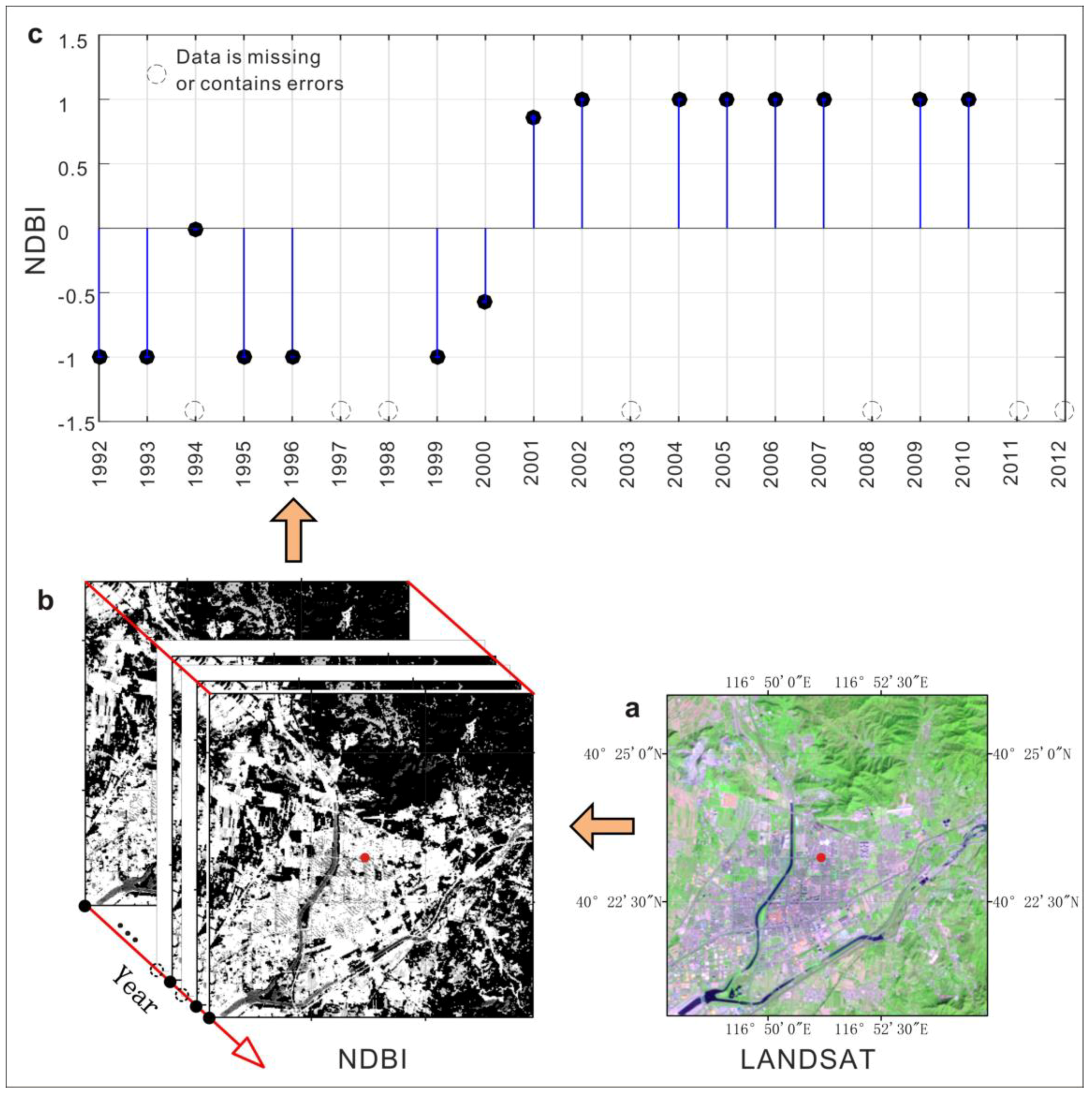
Figure 1a shows the Landsat image covered by Path 123 and Row 32 (false color composite in which bands 7, 4 and 3 are displayed as red, green and blue). Figure 1b shows the NDBI images derived from the radiometrically corrected images. In the NDBI image, the built-up land features are greatly enhanced with a light gray to white tone, while vegetation areas are considerably suppressed with a dark gray to black shade. This owes to the enlargement of the contrast between built-up land and vegetation by the NDBI. Figure 1c is time-series NDBI value of the experimental point, which is located at 116°51′18.6″ E and 40°23′16.8″ N.

Time series Landsat data cannot be used directly to identify the construction year of the buildings because the data had quality, quantity and timing errors. Generally speaking, Landsat data have the following drawbacks: (1) Landsat data often experience technical problems with seemingly random data loss, including the so-called “Christmas tree” anomaly or dropped scans and sun-glint anomaly; (2) most optical remote sensing images include clouds and associated cloud shadows which obscure the detection of land surface, reducing the availability of usable Landsat data and resulting in the restriction of the time series analysis in the built areas of this study. For example, in the 40 cities in the study it was found that entirely cloud-free images of an entire city area are rare, while partial coverage is more frequent; (3) in 2003, the permanent failure of a component of the Landsat 7 ETM+ optical scanning system (called the scan line corrector or “SLC”) resulted in a wedge-shaped gap that accounts for about 25 percent of missing data pixels per image [34]. Although some damaged images can be substituted with those from Landsat 5, others lack an alternative or are unavailable for other reasons; (4) according to the Earth Resources Observation & Science Center of the US Geological Survey (EROS-USGS), there may be data that were collected by the sensor but not archived or distributed. These altogether make it difficult to conduct this study using conventional methods. First, land cover maps cannot be used for change detection because errors from (1) and (2) will significantly decrease the likelihood of detecting temporal change [35] and thus lower the accuracy. Second, due to gaps caused by (3) and (4), the temporally discontinuous land cover maps will reduce temporal resolution below once per year. To solve such problems, the construction year of the buildings is identified based on a Normalized Difference Built-up Index (NDBI) logistic model.

NDBI is one of several widely used indices which is sensitive to the built-up area [36,37]. The equation for NDBI is as follows:

$$NDBI=\frac{B5-B4}{B5+B4}$$

(2)

where B5 and B4 are shortwave infrared band (SWIR, band5) and near-infrared band (NIR, band4) of the Landsat images, respectively. The index development was based on the unique spectral curve in built-up areas: the reflectance in the SWIR wavelength range is higher than that in the NIR wavelength range. It can be seen in Figure 1b that built-up areas experience a drastic increment in their reflectance from NIR to SWIR, resulting in positive values for built-up pixels which can be clearly separated from the remaining covers of close to 0 for vegetation. Unlike the conventional threshold application of NDBI, where a certain range of values from the index raster is used to find a typical feature of interest (in many case studies, the threshold is set at zero and thus the positive values of NDBI represent the built-up area), this study utilized continuous values rather than discretizing the original data set. The greater the NDBI value of a pixel, the higher the possibility of the pixel being a built-up area. Therefore, during a building construction cycle, NDBI will shift from a steadily low value period and finally reach a high value period and remain at that level. A logistic model was used to simulate and reconstruct NDBI time series since such model best fits the values [38,39]. 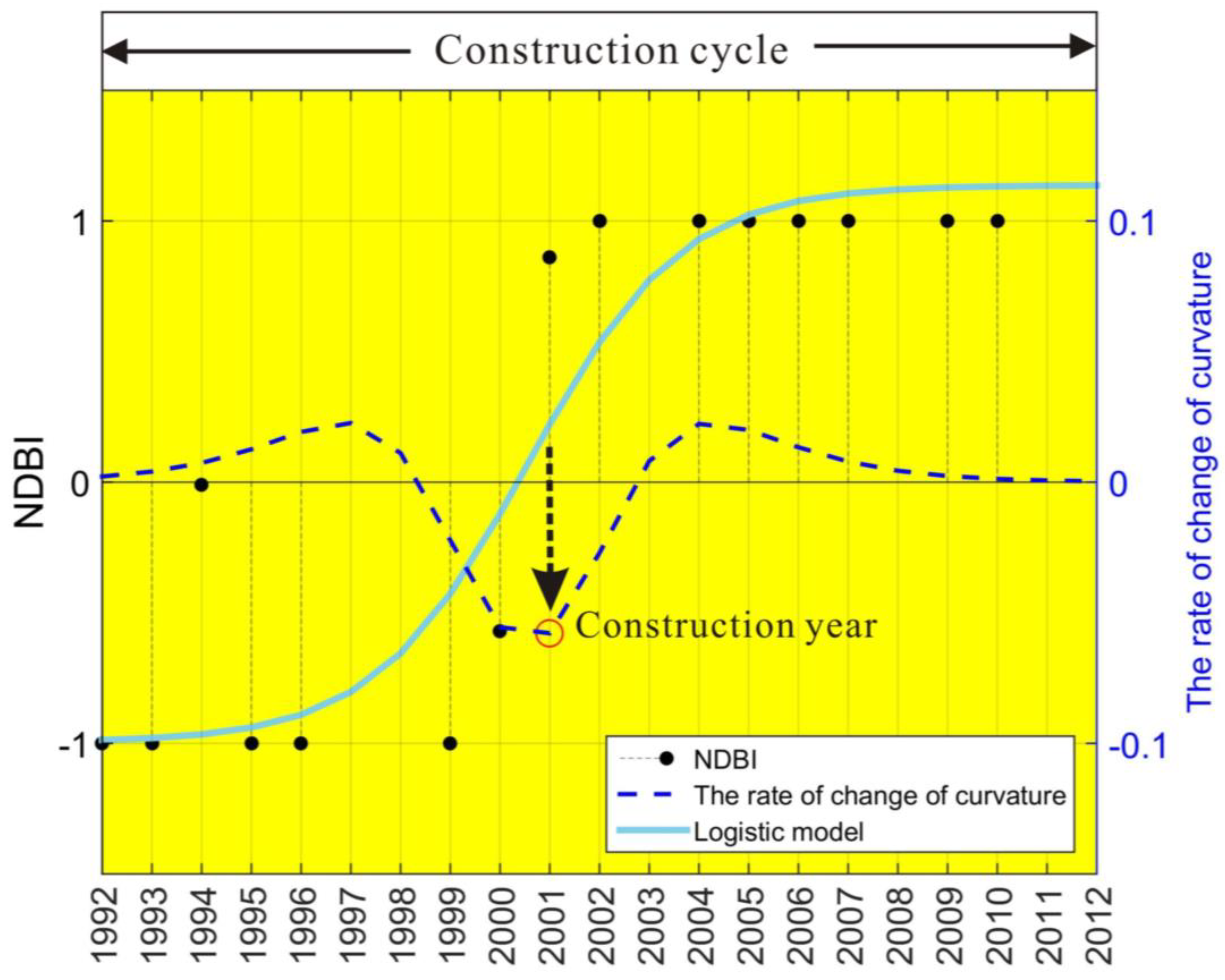Another unique attribute of the logistic model of time is its ability to determine the construction year of the buildings through the inflection point of the curve, which represents the main inversion phase in the cycle (Figure 2).

Black solid points represent annual values of NDBI in newly built areas (see Figure 1). The solid blue line is the fitted logistic model and the dashed black line is the rate of curvature change of the model. The red circle is the minimum point indicating the construction year.

Time series NDBI can be modeled using the following equation:

$$y\left(t\right)=\frac{c}{1+e^{a+bt}}+d$$

(3)

where t is the year, y(t) is the NDBI value at year t, a and b are fitting parameters, c + d is the maximum NDBI value and d is the initial background NDBI value. The fitting parameters a and b were determined using least-square fitting.

Before the NDBI could be fit to the logistic model described by Equation (3), it was necessary to smooth the data through a Savitzky-Golay filter (SG), which both smooths and computes derivatives of a set of consecutive values. Based on an asymmetric Gaussian function fitting, the design concept of SG is to find a suitable filter coefficient to both remove random noise and protect the high-order movement [40]. Rather than a constant, the local quadratic polynomial is utilized for the least-squares fitting within a moving window. Taking a fixed number of points in the vicinity point to fit a polynomial, SG gives the smooth value of the vicinity point according to the polynomial during the fitting progress. The equation of the fitting process can be given as follows:

$$NDBI(t)=\frac{{\displaystyle {\sum }_{i=-m}^{i=m}{C}_{i}NDB{I}_{j+1}}}{N}$$

(4)

where NDBI(t) is the fitted NDBI value, C_i is the coefficient for the ith NDBI point of the filter, N is the number of convoluting integers equal to the smoothing window size (2 m + 1) and j is the running index of the original ordinate data table. During the process, invalid points affected by external factors in the NDBI time series show abnormally low or high values and these will be eliminated during the SG filter process.

The local minimum point of the fitted logistic model divided NDBI into sustained increasing and decreasing trends. Since the construction year of the building corresponds to the point at which the rate of change in curvature exhibits the local minimum, it is defined as the year when the second derivative shifts from negative to positive values [38]. The curvature 𝐾 for Equation (4) at year 𝑡 can be computed by:

$$K=\frac{d\alpha }{ds}=-\frac{b^{2}cz\left(1-z\right){\left(1+z\right)}^3}{{\left[{\left(1+z\right)}^4+{\left(bcz\right)}^2\right]}^{\frac{3}{2}}}$$

(5)

where $z=e^{a+bt}$, a is the angle of the unit tangent vector at year t along a differentiable curve and s is the unit length of the curve. The rate of change of curvature $K^{\prime }$ can be computed by the following equation:

$$\begin{array}{l}{K}^{\prime }=b^{3}cz\left\{\frac{3z\left(1-z\right){\left(1+z\right)}^3\left[2{\left(1+z\right)}^3+b^2{c}^{2}z\right]}{{\left[{\left(1+z\right)}^4+{\left(bcz\right)}^2\right]}^{\frac{5}{2}}}-\frac{{\left(1+z\right)}^2\left(1+2z-5z^2\right)}{{\left[{\left(1+z\right)}^4+{\left(bcz\right)}^2\right]}^{\frac{3}{2}}}\right\}\end{array}$$

(6)

2.3. Nighttime Light’s Rate of Change in Newly Built Area

Nighttime light’s rate of change in newly built area (NLRCNBA) is used to assess a city’s darkness according to the following formula:

$$NLRCNB{A}_t=\frac{n\times {\displaystyle {\sum }_{i=1}^n(i\times D{N}_i)}-{\displaystyle {\sum }_{i=1}^{n}i}{\displaystyle {\sum }_{i=1}^{n}D{N}_i}}{n\times {\displaystyle {\sum }_{i=1}^n{i}^2-{({\displaystyle {\sum }_{i=1}^{n}i})}^2}}$$

(7)

where i is the year sequence from 1992 to 2012; n is the number of years; t is the construction year of buildings; DN is the DMSP/OLS value; and NLRCNBA_t denotes the nighttime light’s rate of change in a newly built area for year t. Since NLRCNBA_t indicates the mean temporal change of the interannual variation of the DMSP/OLS value in a newly built area for construction year t, the yearly NLRCNBA change directly reflects the dynamic of darkness in a newly built area. 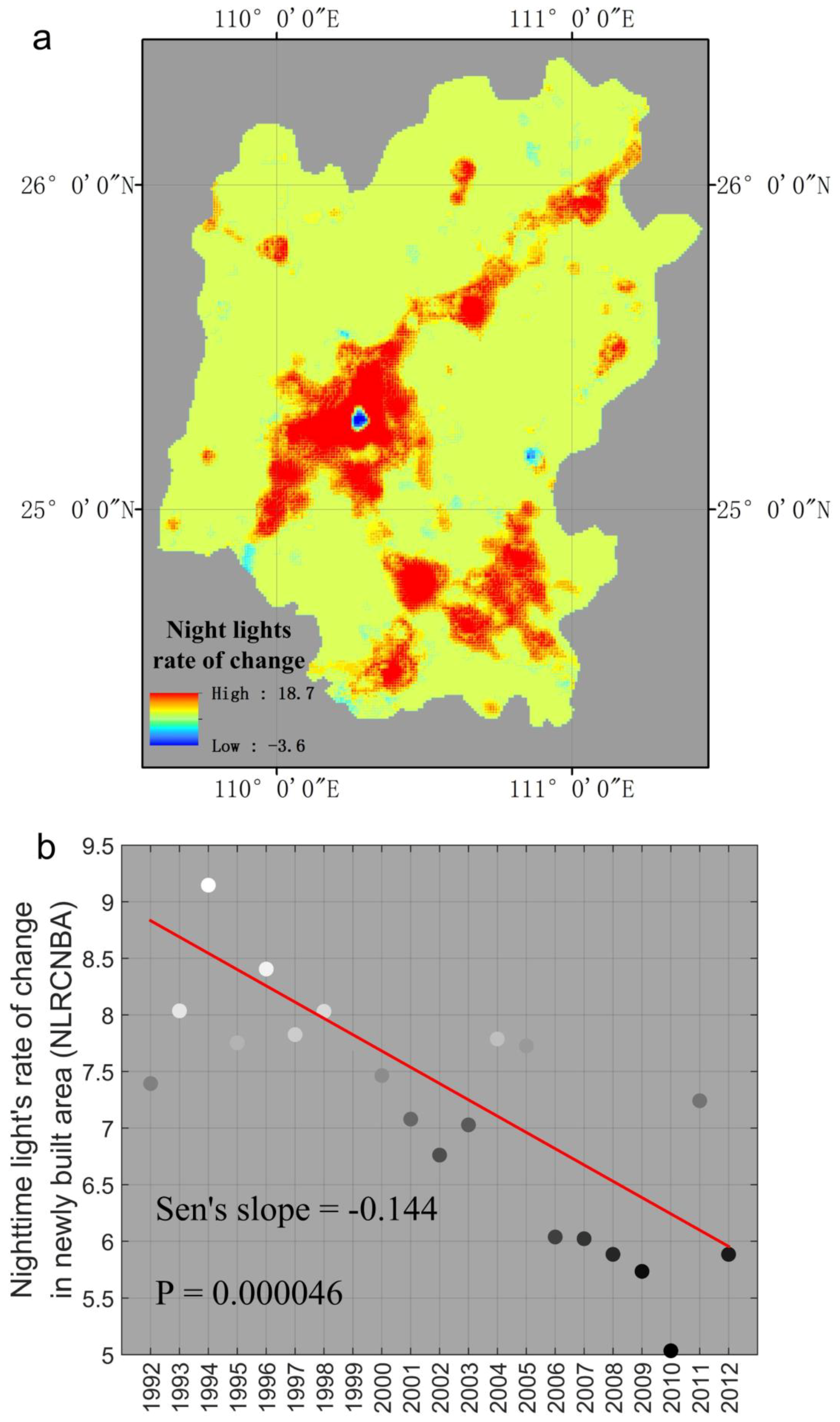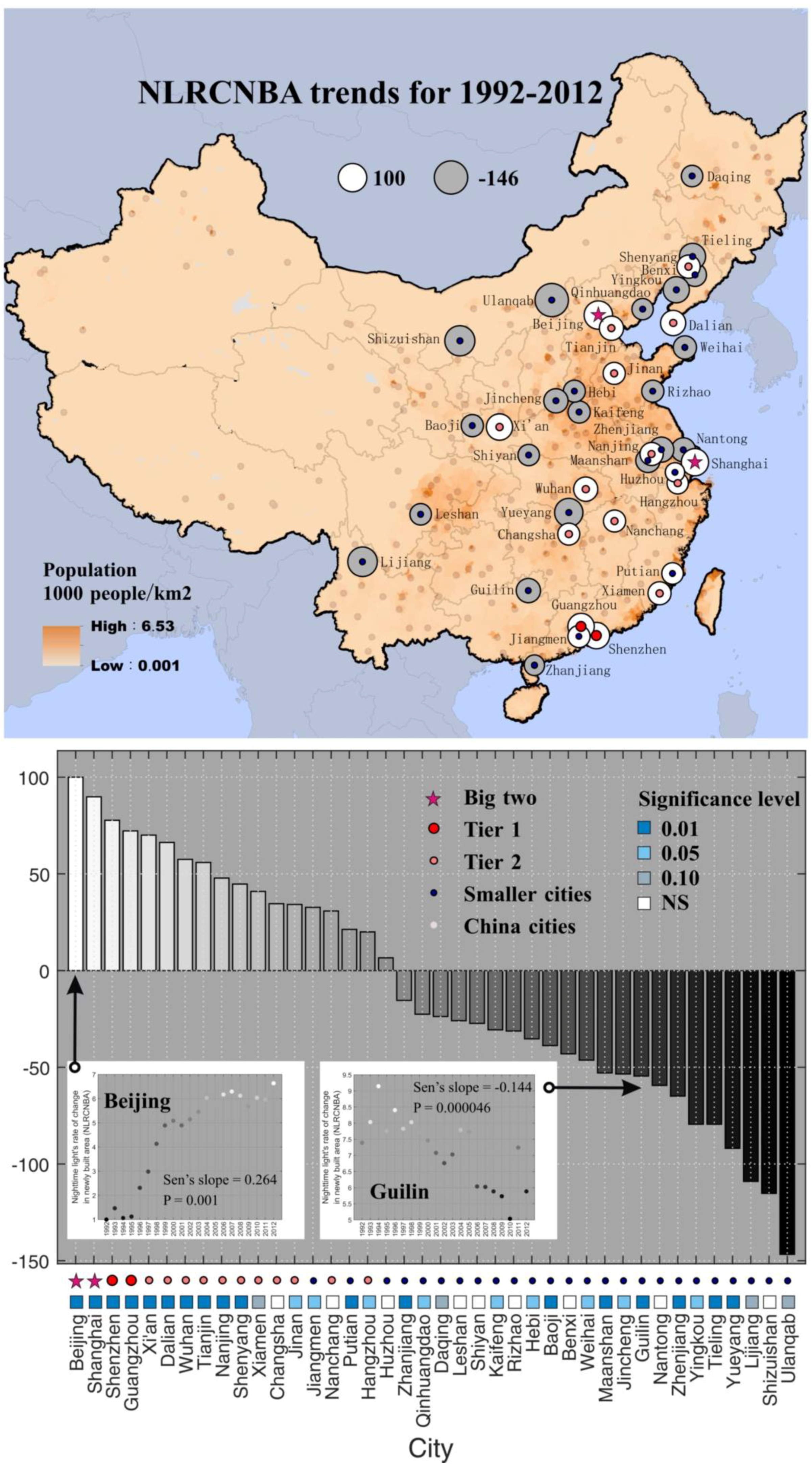Therefore, the NLRCNBA trend, as a result of residential activities in a newly built area, is an appropriate indicator for ghost cities: if the trend >0, the city is brighter and the intensity of residential activities in new buildings increases; otherwise, the city becomes darker and the intensity of residential activities in new buildings decreases. In this study, the statistical significance of trends was assessed based on Mann-Kendall test and Sen’s slope was used to evaluate the NLRCNBA trend.

The Mann-Kendall (MK) test is a non-parametric statistical procedure that is well suited to analyzing trends in data over time [41,42]. One advantage of this test is that the data need not conform to any particular distribution. The second advantage of the test is its low sensitivity to abrupt breaks due to inhomogeneous time series. As a result, the time series of NLRCNBA values of cities were analyzed for monotonous increasing or decreasing trends using the MK test.

Along with the Mann-Kendall test, Sen’s slope calculation was determined. Unlike linear regressions, Sen’s slope test is a nonparametric, linear slope estimator that works most effectively on monotonic data. Similar to the MK test, the advantage of Sen’s slope estimator is that it is largely unaffected by gross data errors, outliers, or missing data. Therefore, it is more rigorous than most regression slopes and provides a more realistic measure of the trends in the NLRCNBA series. Simply speaking, Sen’s slope is the median of all differences between successive data values [43,44].

2.4. Validation

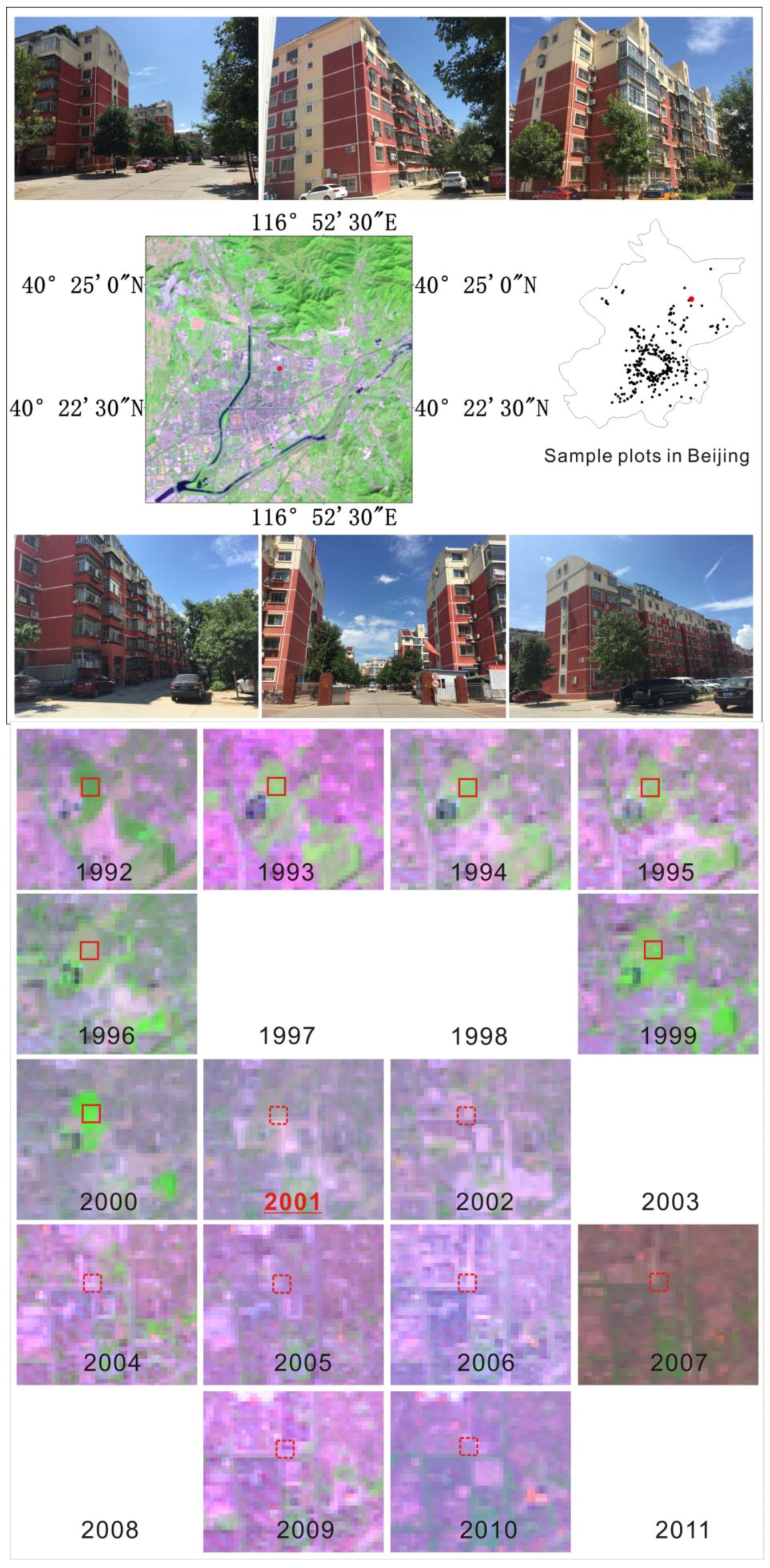
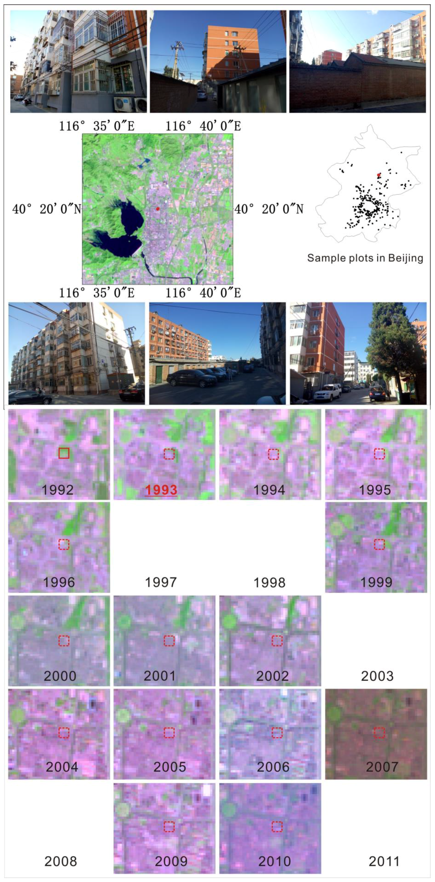
Figure 3 shows two sample plots in Beijing, located at 116°51′18.6″ E and 40°23′16.8″ N and 116°38′7.3″ E and 40°20′6.3″ N, respectively. Photos were taken during field survey. In the time series Landsat color composite images (false color composite in which bands 7, 4 and 3 are displayed as red, green and blue) the solid rectangle indicates vegetated area and the dashed rectangle indicates that was converted to built-up area. The construction year of the building is labeled as red text.

An analysis of the achieved accuracy to detect the construction year of the building was performed by extracting a set of sample plots and visually inspecting the results in those plots. The validation phase was conducted by stepwise procedure, as follows: (1) Sample plots were extracted using a random sampling method to represent the variability within the plot sample [45]. The number of sample plots required for accuracy assessment depends on the minimum level of accuracy required. Jensen discusses an equation suitable for determining a minimum number of pixels required for different levels of accuracy [46], as follows:

$$N=\frac{4p(1-p)}{E^2}$$

(8)

where N is total number sample plots, p is expected percent accuracy and E is allowable error. Here p was adopted as 80 percent and E was adopted as ±5 percent and thus N = 256. Finally, 300 sample plots were used for accuracy assessment. (2) The results of the construction year were assessed by comparison with the time series Landsat color composite images and field survey (Figure 4).

To remove noise and disturbance, city areas were masked out using two vector polygons which define the urban outline in 1992 and 2012 and only the built-up lands inside the 2012 urban region and outside the 1992 urban region were retained as newly built area. In Beijing, the overall accuracy of the logistic model in identifying the construction years of buildings was 73.6 percent with disagreements on 79 points. This discrepancy mainly occurred in mixed urban areas, which are strongly affected by the low separability between agricultural or vegetated areas and buildings. Such fragmentation and variety caused falsity in 51 points. The other 28 failures can be attributed to data inconsistency from time-series Landsat images. Overall, the validations show that the method can provide correct and reliable results with a satisfactory level of accuracy.

3. Results

3.1. A Case of NLRCNBA Trend

Figure 4a shows the nighttime light’s rate of change from 1992 to 2012 in Guilin City, Southwest China. Figure 4b shows years against the nighttime light’s rate of change in newly built areas. The null hypothesis (Ho) is that no change or trend has occurred in NLRCNBA over time. Hence the alternate hypothesis (Ha) is that a significant change has occurred over time, or that an increasing or decreasing trend in NLRCNBA is present. In this case, there is a very small p-value of 0.000046 from Mann-Kendall test, which is much less than a significance level of 0.01 (corresponding to a 99 percent confidence level), resulting in a high weight of evidence against the null hypothesis (Ho). So, Ho is rejected, or it is accepted that a change of the nighttime light rate of change in a newly built area has occurred over time.

Taking Guilin City as a case study, the nighttime light’s rate of change was positive in almost all areas, with the result that the map color (Figure 4a) is predominantly red or yellow rather than blue. However, despite such generally increasing trends, in newly built areas, the slope of the rate of change is negative (Sen’s slope = −0.144 in Figure 4b). This negative value, which measures the rate of change in current newly built areas as opposed to that in newly built areas a certain number of years ago, indicates continuous and significant decrease year by year. As a result, the intensity of residential activities in new buildings in Guilin weakened over the 21-year time period.

3.2. China’s Ghost Cities

Figure 5 shows Sen’s slope for 1992–2012 in China’s 40 cities for NLRCNBA, ranging from 100 to −146.6. Taking Beijing’s value as 100, Shanghai’s was 89.8, Shenzhen’s was 77.65 and Guangzhou’s was 72.35 and their trend values ranked 1st, 2nd, 3rd and 4th, respectively. All big cities in Group B show positive values and most of the smaller cities in Group A show negative values.

For evaluating China’s ghost cities, Sen’s slope was used with the Mann-Kendall test to estimate the magnitude of NLRCNBA trend. In 19 cities, the NLRCNBA trends were positive, including all the “big two” cities and all Tier 1 and Tier 2 cities (Figure 5). In contrast, most smaller cities in our study showed negative values. The result indicates that during 1992–2012, residential activities in smaller cities tended to decrease, resulting in the cities’ newly built areas remaining virtually dark and deserted (

Table 2. Sen’s slope, Mean Kendall statistic, normalized test statistic and p-value for 1992–2012 in China’s 40 cities.

Tier	City	Mean Kendall Statistic (S)	Normalized Test Statistic (Z)	p-Value	Result	Sen’s Slope	Trend Direction
Big Two	Beijing	172	5.164	0.000	Trend exists	0.264	⇧
	Shanghai	54	3.233	0.001	Trend exists	0.237	⇧
Tier 1	Guangzhou	126	3.775	0.000	Trend exists	0.191	⇧
	Shenzhen	94	2.808	0.005	Trend exists	0.205	⇧
Tier 2	Shenyang	108	3.231	0.001	Trend exists	0.118	⇧
	Hangzhou	82	2.446	0.014	Trend exists	0.053	⇧
	Tianjin	86	2.567	0.010	Trend exists	0.148	⇧
	Dalian	128	3.835	0.000	Trend exists	0.175	⇧
	Wuhan	108	3.231	0.001	Trend exists	0.152	⇧
	Nanjing	134	4.016	0.000	Trend exists	0.126	⇧
	Xiamen	64	1.902	0.057	Trend probably exists	0.108	⇧
	Xi’an	112	3.352	0.001	Trend exists	0.185	⇧
	Changsha	48	1.419	0.156	-	0.091	⇧
	Jinan	72	2.144	0.032	Trend exists	0.090	⇧
	Nanchang	42	1.238	0.216	-	0.081	⇧
Smaller cities	Qinhuangdao	−68	−2.023	0.043	Trend exists	−0.060	⬇
	Jincheng	−66	−1.963	0.050	Trend exists	−0.141	⬇
	Benxi	−45	−1.539	0.124	-	−0.114	⬇
	Yingkou	−76	−2.265	0.024	Trend exists	−0.210	⬇
	Tieling	−91	−2.718	0.007	Trend exists	−0.210	⬇
	Daqing	−64	−1.902	0.057	Trend probably exists	−0.063	⬇
	Nantong	−48	−1.419	0.156	-	−0.157	⬇
	Zhenjiang	−120	−3.593	0.000	Trend exists	−0.171	⬇
	Huzhou	38	1.117	0.264	-	0.017	⇧
	Maanshan	−98	−2.929	0.003	Trend exists	−0.140	⬇
	Weihai	−68	−2.023	0.043	Trend exists	−0.122	⬇
	Rizhao	−44	−1.298	0.194	-	−0.082	⬇
	Kaifeng	−80	−2.386	0.017	Trend exists	−0.081	⬇
	Hebi	−72	−2.144	0.032	Trend exists	−0.093	⬇
	Shiyan	−40	−1.178	0.239	-	−0.072	⬇
	Yueyang	−140	−4.197	0.000	Trend exists	−0.243	⬇
	Jiangmen	68	2.023	0.043	Trend exists	0.086	⇧
	Putian	90	2.688	0.007	Trend exists	0.056	⇧
	Zhanjiang	−96	−2.869	0.004	Trend exists	−0.041	⬇
	Guilin	−136	−4.077	0.000	Trend exists	−0.144	⬇
	Leshan	−48	−1.419	0.156	-	−0.068	⬇
	Lijiang	−64	−1.902	0.057	Trend probably exists	−0.288	⬇
	Baoji	−124	−3.714	0.000	Trend exists	−0.102	⬇
	Shizuishan	−41	−1.515	0.130	-	−0.304	⬇
	Ulanqab	−43	−1.732	0.083	Trend probably exists	−0.387	⬇

Note: Z for a confidence interval of 99 percent, 95 percent and 90 percent to be 2.58, 1.96 and 1.645, respectively.

).

The significance level (α) is the probability of concluding whether there is a NLRCNBA trend when none actually exists. A significance level of 0.10 is considered a conservative approach so that the analysis is sensitive to possible changes in NLRCNBA over time. Significance levels (α) were divided into three sub-levels: 0.01, 0.05 and 0.1. A lower significance level decreases the chances of erroneous indication of a NLRCNBA trend, or indicates that a NLRCNBA trend is more likely to occur. It was found that, for the 15 big cities of Group B, the significance levels were less than 0.10, except Changsha and Nanchang. Furthermore, the big two cities and Tier 1 cities all dipped below the 0.01 level and eight cities (72 percent of the total) in Tier 2 were less than 0.05. Compared to Group B, the smaller cities of Group A showed more diversity: eight cities passed the 0.01 level, seven cities passed the 0.05 level and three cities passed the 0.10 level, accounting for 32 percent, 28 percent and 12 percent of the total, respectively.

Figure 6a illustrates differences of the coefficient of determinations (R2) between the linear regression model and the nonlinear regression model of second-order polynomial in big cities; 6b illustrates the peak years in descending order; in 6c, the solid blue lines are the second-order polynomial regression model and the dashed red lines are peak years according to the roots of the derivative; and 6d illustrates NLRCNBA trends for 2007–2012 based on their real values.

Two regression models were tested to define the distribution of NLRCNBA in terms of years in big cities: a linear regression model and a nonlinear regression model of second-order polynomial (Figure 6). It was found that the coefficient of determinations (R²) in the nonlinear regression model of second-order polynomial were significantly higher than in the linear regression model. This was especially true in lower-ranking cities. For example, the coefficient of determinations (R²) increased significantly from 0.25 to 0.51 for Hangzhou, from 0.19 to 0.75 for Changsha and from 0.14 to 0.68 for Nanchang. Higher R² levels suggest that the linear regression model, where NLRCNBA is directly proportional to the amount of years, is no longer applicable or appreciate. Thus, a second-order polynomial regression model better fits the data, resulting in high coefficients of determination values (R²) of 0.94, 0.86, 0.74, 0.51, 0.74, 0.85, 0.75 and 0.68 for the cities of Beijing, Shanghai, Guangzhou, Hangzhou, Wuhan, Xi’an, Changsha and Nanchang, respectively. In these cities, this model presents a maximum value for NLRCNBA. Because of this effect, the response of NLRCNBA against a specific year reached a finite amount. The peak years corresponding to maximum NLRCNBA values were detected by finding the roots of the derivatives. It was found that when a city’s ranking decreased, its peak year accordingly advanced (in this case, from 2009, 2007, 2005 to 2003 in Figure 6b). A second-order polynomial regression model will fall after reaching the peak year, resulting in a descending trend. 2007 was regarded as a starting year and it was confirmed that NLRCNBA trends, based on their real values, were negative in recent years.

4. Discussion

The ghost city problem is real but so far appears to be concentrated in smaller cities undergoing an economic shift, or where the local economy is heavily dependent on natural resources, industries, tourism, or farming. For example, the city of Ulanqab ranks as the first negative value on Sen’s slope. Ulanqab has a very unbalanced economic system, with 53.1 percent of the population relying on farming and animal husbandry [47]. It is also too remote and cold to attract immigrants. Shizuishan, a resource-exhausted city relying on its coal mines in Northwest China’s Ningxia Hui autonomous region, is ranked second. Other resource-exhausted cities include Benxi, Daqing, Hebi, Jincheng, Maanshan, Tieling and Yinkou. The third city, Lijiang, is a popular tourist destination, resulting in a largely transient population. Other tourist hotspots include Guilin, Qinhuangdao, Kaifeng and Weihai.

Other cities, like Baoji, Leshan, Nantong, Rizhao, Shiyan, Yueyang, Zhanjiang and Zhenjiang, are implementing arduous measures to catch up with the country’s economic development. All these ghost cities are generally characterized by a large number of urban renewal programs and expansion, or are brand new cities whose economies are not diversified enough to offer a wide range of employment opportunities to attract a sustainable inflow of migrants.

The results from big cities show a completely different situation: trends over time are all positive. Such positive trends can be partially verified by a 2013 CLSA survey that covered 800,000 apartments in 12 cities and found that the vacancy rate in big cities was just 10 to 16 percent, as opposed to 20 to 30 percent in smaller cities [13].

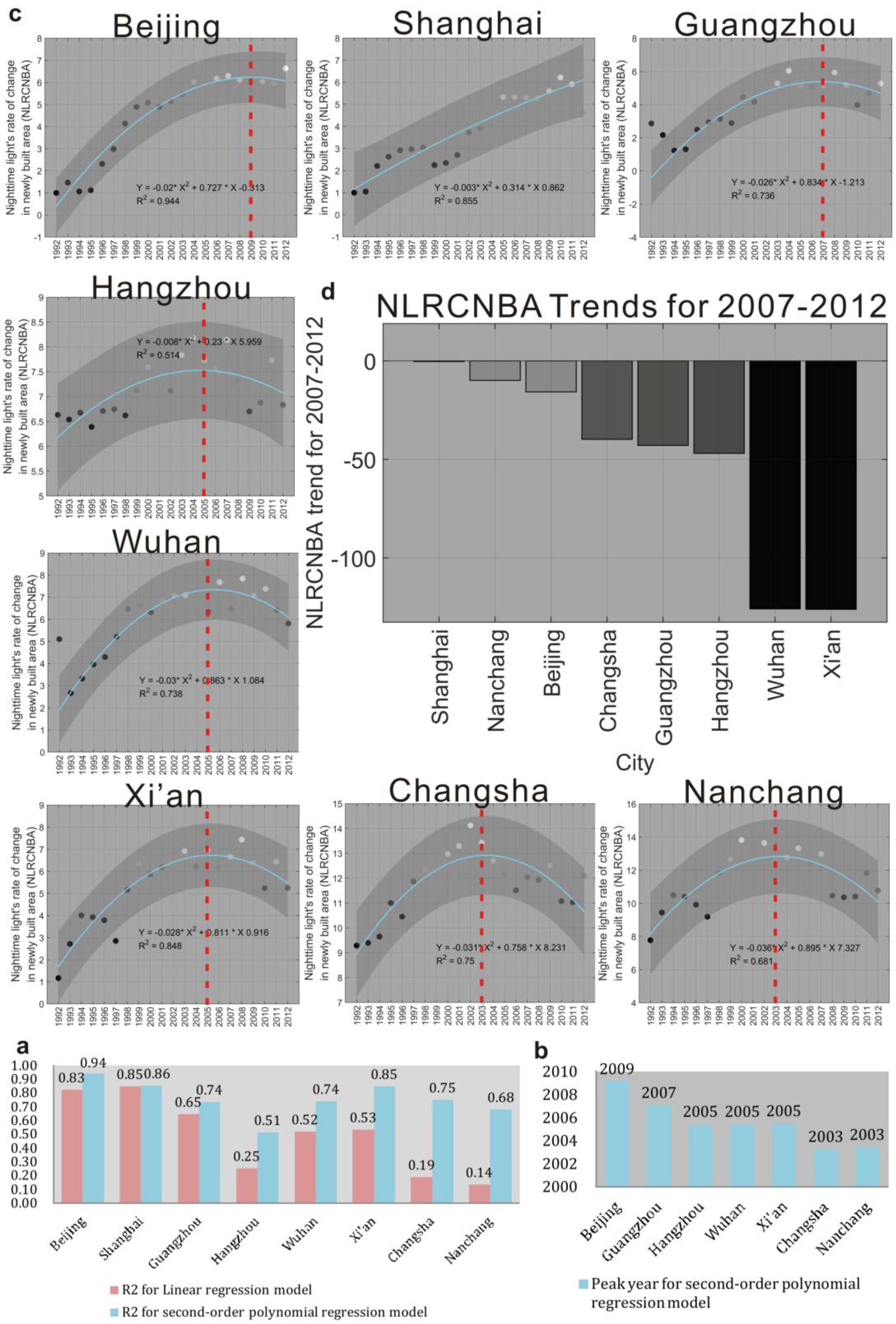
Similar to a Kuznets model [48], big cities in our study followed an inverted U curve that graphs NLRCNBA against time, over the course of each city’s economic development. In this period, the data shows an increase in nighttime light, which peaks and then falls. This curve has a number of implications. The left side of the curve illustrates that as an economy develops and creates more jobs in a city, the pace of home sales begins to accelerate. Here, many people are buying new houses in conjunction with large-scale migration. This results in a positive NLRCNBA trend. At this stage, the land boom leads to a rapid increase in property valuation.

The right-hand side of the curve shows the decline of home sales after the peak. When valuations of real property reach unaffordable levels for most people, or there is an economic slump, the number of unsold homes is higher and housing demands is lower. As a result, the NLRCNBA trend begins to show up negative. This describes the current situation in China’s big cities, with a steady drop in the number of homes sold.

The middle of the curve shows when NLRCNBA reaches its peak. Our study highlights how the peak years vary as the cities’ ranking varies—the higher a city’s rank, the later its peak year. This means that high tier cities are the concentration of China’s economic strength and the demand for commercial real estate in high tier cities is much stronger than that in low tier cities. The National Bureau of Statistics reported that in 2015, average home prices in China’s four largest cities of Beijing, Shanghai, Guangzhou and Shenzhen, where supply is scarce, grew much faster than the other 66 communities surveyed. Meanwhile, many smaller communities still suffer from large inventories of unsold homes [49].

Still, it remains a major challenge to conduct the assessment on mapping China’s ghost cities. Several limitations and uncertainties associated with this study are as follows. First of all, the study was restricted to 25 smaller and 15 larger cities in China for 1992–2012 due to the available year of DMSP/OLS and data quality of Landsat. Second, a model of quadratic regression was used to calibrate time series nighttime lights data but there are still uncertainties during the procedure. Third, the loss in time series NDBI could introduce errors, although a logistic model with fitting parameters was used to reconstruct the values. In addition, this study cannot quantify the buildings with weak nighttime lights since lights from these buildings are below the threshold of DMSP/OLS.

Approaches based on new data sources for dealing with these limitations and uncertainties could be developed in order for the measurement and reporting of ghost cities to be more successful. The Visible Infrared Imaging Radiometer Suite (VIIRS), which enables a new generation of operational moderate resolution-imaging capabilities since November 2011, collects imagery and radiometric measurements of the land, atmosphere, cryosphere and oceans in the visible and infrared bands of the electromagnetic spectrum [50]. Since the VIIRS instrument collects the same spectral bands as Landsat plus low light imaging data similar to DMSP from a single sensor, it may be possible to produce the most recent (2012–present) ghost city maps in a simple way. Furthermore, to overcome data quality barriers of Landsat, MODIS data could be used to calculate NDBI back to year 2000. As a result, national wide ghost city map could be produced through the combination of DMSP/OLS nighttime lights and MODIS-based NDBI.

5. Conclusions

As Chinese cities pursue economic growth through urbanization and thus implement ambitious land development projects, some of them have inadvertently turned themselves into ghost cities. Traditional social-economic statistical data based on the household surveys in China is insufficient to conduct in-depth research into such social-economic phenomenon. A number of researches apply remote sensing to characterize urban extent, monitor the dynamics of urban expansion and evaluate associated environmental impacts. For example, DMSP/OLS data covering two decades is widely used to determine the spatiotemporal dimensions of socio-economic factors, while Landsat satellite images allows a detailed study of natural and human-induced changes on the global landscape. Although, any of these data sets, when used by themselves, is not the best way to settle this problem, the combination of these datasets has a unique capacity to capture the size, growth, level, distribution, scale, intensity and pattern of China’s ghost city. As proven in this research, residential activities decline in newly built areas of smaller cities in China, leading to what are known as ghost cities. At night, uninhabited housing units with few lights appear dark—a sign that few people live there.

One particularly important result from this work is that our results provide a new perspective towards increased usage of multiple sources of remotely sensed data, especially the complementary data source in urban area. Previous researches focus on the complementary characteristics in space, for example, vegetation area and built up area based on MODIS products and DMSP/OLS data. A case is that the DMSP-OLS and Terra MODIS NDVI data were combined to develop a settlement index image to estimate fractional settlements from coarse spatial resolution images at the regional scale by combining a limited number of medium spatial resolution images [51]. Other research [52] indicates that despite the uncertainties in sensor fusion and the coarse resolution of the data, the combination of MODIS products such as NPP with nighttime data could provide rapid assessment of urban land cover changes and their impacts on regional ecosystem resources. In this study, the complementary characteristics in time between nighttime remotely sensed data and daytime remotely sensed data can contribute to enrich, extend and widen the topic and therefore well provide more representative characterization of land use and demographic geospatial patterns from rapid urban spatial-temporal changes, for example, ghost cities. It was found that 22 smaller cities can be categorized as ghost cities and nighttime lights change in newly built areas following an inverted U-curve for big cities.

The logical extension of this work will be to apply the methodology in other areas, especially in developing countries which are currently experiencing as sizeable growth rates of urban concentration due to rapid population growth and economic transformation by a combination of rapid technological and political change [24,53] as in China. How to quantify side effects of urbanization at a regional level, such as ghost cities, are essential for policy makers to put forward countermeasures to solve them. Doing so will require a variety of reliable and well-established information, including their spatial-temporal pattern. But lack of the financial and/or institutional resources to conduct all-round and in-depth censuses in these countries results in unavailability and poor quality of the statistical data. In particular, our methodological approach would well detect residential activities change in newly built areas via nighttime satellite data and daytime satellite data and thus allow policy makers to track the spatial pattern and temporal evolution of ghost cities. This is of great significance in upgrading urban management level, implementing efficient urban administration and achieving the strategic goal of urban sustainable development.