A Preprocessing Method for Hyperspectral Target Detection Based on Tensor Principal Component Analysis

Abstract

Traditional target detection (TD) algorithms for hyperspectral imagery (HSI) typically suffer from background interference. To alleviate this problem, we propose a novel preprocessing method based on tensor principal component analysis (TPCA) to separate the background and target apart. With the use of TPCA, HSI is decomposed into a principal component part and a residual part with the spatial-spectral information of the HSI being fully exploited, and TD is performed on the latter. Moreover, an effective distinction in scheme can be made between a HSI tensor’s spatial and spectral domains, which is in line with the physical meanings. Experimental results from both synthetic and real hyperspectral data show that the proposed method outperforms other preprocessing methods in improving the TD accuracies. Further, target detectors that combine the TPCA preprocessing approach with traditional target detection methods can achieve better results than those of state-of-the-art methods aiming at background suppression.

1. Introduction

Hyperspectral remote sensing for earth observation has attracted increasing interest in recent years. In addition to the ground cover’s spatial distribution, hyperspectral imaging sensors can synchronously measure the reflectance of materials in hundreds of narrow and contiguous bands, spanning over the visible-to-infrared and even a wider range of the electromagnetic spectrum [1,2]. Therefore, each pixel of hyperspectral imagery (HSI) can be presented as a continuous spectral curve. HSI has been extensively applied in various fields, such as mineral exploration, environmental protection, and military affairs [3,4,5].

Target detection (TD) is one of the most important HSI processing technologies [6,7]. Different materials usually have distinct wavelength-dependent electromagnetic scattering and radiation characteristics, which essentially enables TD for HSI. In fact, TD is about solving a supervised dichotomous problem where pixels are labeled the target or background according to their similarity to a priori target spectra.

In recent decades, many TD algorithms have been developed. The probability and statistics-based model is one of the classic models for TD, and some traditional TD algorithms in the literature are proposed based on it. For example, constrained energy minimization (CEM) [8] is a finite impulse response filter which minimizes the total output energy, subjected to the constraint that the output of the target’s spectral signature is one. In general, CEM can well distinguish the targets from background. The adaptive cosine/coherence estimation (ACE) [9] and the adaptive matching filter (AMF) [10] algorithms are based on Kelly’s generalized likelihood ratio detection operator. An assumption is made in these two detectors that a mixed background model is subject to the multivariate Gaussian distribution, and additive noise has already been included in the background. Generally, ACE and AMF detectors can be deduced from the generalized likelihood ratio test (GLRT). Closed-form solutions and a considerably low computational cost for TD can be usually achieved with these algorithms. Equipped with the characters above, CEM, ACE and AMF are commonly cited as classic TD methods in many works related to TD [11,12,13].

In fact, a vast majority of HSI pixels often belong to the background, while the target only presents in a few of pixels. The aforementioned methods commonly suffer from background interference, which may give rise to false alarms. Therefore, it is very important to improve the performance of the target detection algorithm by minimizing the interference of background pixels.

Several state-of-the-art hyperspectral target detection techniques have been proposed to cope with this issue. Two types of methods, i.e., background suppression and background separation, are usually considered. The hierarchical constrained energy minimization (hCEM) method [14] consists of different layers of classic CEM detectors, and the output of each layer is considered as the coefficient of the next layer to suppress the background. The geometric matched filter (GMF) method [15,16] provides an inventive way to suppress the background by estimating the background endmembers. Both hCEM and GMF detectors are adept at suppression of the undesired background, which enables them to better concentrate on the targets and acquire remarkable detection results.

Apart from background suppression, background separation also plays an important role in minimizing the background interference and has drawn increasing interest. It is thus very meaningful to develop a preprocessing method aiming at separating the background and target apart before TD is performed. Principal component analysis (PCA) [17] can be used to address this problem and decompose the HSI into a principal component (PC) part and a residual part. The background is supposed to mainly exist in the PC part, while the target is regarded to present in the residual part. Another famous method, independent component analysis (ICA), which is an unsupervised blind source separation technique has also already been used in hyperspectral data processing [18] and background separation [19]. ICA can separate endmembers apart, which enables its application in hyperspectral target detection. Nevertheless, ICA only shows independent sources instead of signal intensity, which makes it difficult to discriminate the part containing the target. In this sense, the connection between ICA and our feature extraction preprocessing scheme actually seems to be considerably weak. Therefore, we consider PCA as a feasible approach for background separation.

However, PCA only takes advantage of the one-dimensional spectral features of samples, which signifies the absence of any spatial dimensions. As a result, PCA fails to employ the spatial information of HSI, which has become an inevitable drawback in HSI processing. Unfortunately, the spatial information of HSI is always of great significance. This fact prevents PCA from being a desirable instrument for HSI processing.

Mathematically, a hyperspectral data cube is actually a three-dimensional tensor [20,21]. A tensor can be considered as an extension of a vector and matrix, which provides a convenient way to capture inter-correlation among multiple dimensions. In this sense, both the spectral and spatial domains of hyperspectral datasets can always be better integrated jointly in such an expression than can the situations in two-dimensional matrices. Based on a tensor model, Tucker decomposition [22,23] can take spatial-spectral information into consideration, but the essential difference between the spatial and spectral domains of HSI is ignored. These two classic feature extraction methods perform poorly in reflecting the HSI’s intrinsic physical properties.

Despite this, algorithms related to tensor have attracted increasing attention in the field of hyperspectral image processing [24,25,26] recently. Tensor principal component analysis (TPCA) has been successfully used for feature extraction in HSI classification [27]. Furthermore, we consider that the TPCA model compared with the PCA and Tucker decomposition models should have much more potential in TD.

The TPCA method is a tensorial counterpart of PCA. Not only can the spatial and spectral information of HSI can be considered jointly, but they are also dealt with discriminatively. In this sense, TPCA can overcome the drawbacks of PCA and Tucker decomposition, leading to a more accurate description of the HSI physical property. Inspired by this, we propose a TPCA-based TD preprocessing method. This method first operates TPCA on HSI, thus the imagery is decomposed into the sum of the principal component imagery and the residual imagery. Since the target only takes up a very small number of pixels, it is often considered to appear in the residual imagery. In this way, the target detection in the residual imagery of TPCA can largely reduce the interference of the background, which belongs to the principal component of the HSI, and produce better detection results. Experimental results demonstrate that by using the proposed algorithm, the background and the target can be well separated, and better TD results can be obtained than those with other feature extraction methods and state-of-the-art methods aiming at background suppression.

The main contributions of our work can be concisely summarized as follows:

(1) A tensor principal component analysis (TPCA) based preprocessing method is proposed for hyperspectral target detection. Due to the decomposition of HSI into a principal part and a residual part for detection, the effect of background interference on detection can be well alleviated.

(2) The spectral and spatial information of HSI is not only employed jointly but is also treated differently in the proposed preprocessing method. This characteristic is especially important for revealing the HSI physical property in detection, which also makes the proposed method have superior performance compared with that of PCA and Tucker decomposition.

(3) TPCA-based detectors that combine the proposed preprocessing method with traditional detectors can significantly improve the performance of TD and can outperform some state-of-the-art TD methods.

Traditional hyperspectral target detectors suffer from background interference; thus, their detection performances are limited. Feature extraction preprocessing methods used for background separation, such as PCA and Tucker decomposition, fail to reveal the physical meaning of the HSI’s spatial or spectral domains. The precise objective of this work is to provide a TPCA-based preprocessing method for TD through which both spatial and spectral information of HSI can be reasonably exploited.

The remainder of this paper is organized as follows. Section 2 reviews the related works. Our TPCA-based target detection algorithm is presented in Section 3. Section 4 shows the experimental results. The discussion is shown in Section 5. Conclusions are drawn in Section 6.

2. Related Works

2.1. Symbols and Notations

Representations of basic notations used throughout the paper are listed in

Table 1. Representations of basic notations.

$R$	Real number space
$R^n$	$n$-dimensional real number space
$R^{m\times n}$	$(m\times n)$-dimensional real number space
$C$	Complex number space
$C^{m\times n}$	$(m\times n)$-dimensional complex number space
$a$	Real number scalar
$x$	Real number vector
$X$	Real number matrix
$\mathcal{A}$	Real number tensor
$X^T$	Matrix transposition
$X^H$	Matrix Hermitian transposition [28]
$x_i$	$i$th entry of vector $x$
$X_{i_1,i_2}$ or ${\left(X\right)}_{i_1,i_2}$	$\left(i_1,i_2\right)$th entry of matrix $X$
${[\mathcal{A}]}_{i_1,i_2,\dots ,i_n}$	$\left(i_1,i_2,\dots ,i_n\right)$th entry of tensor $\mathcal{A}$
${\mathcal{R}}_t$	Tensor space (each element is a tensor of a certain size)
${\mathcal{R}}_t^D$	$D$-dimensional tensor space
${\mathcal{R}}_t^{D_1\times D_2}$	$(D_1\times D_2)$-dimensional tensor space
$x_{tv}$	Tensor vector (vector defined in a tensor space)
$X_{tm}$	Tensor matrix (matrix defined in a tensor space)
${\left(x_{tv}\right)}_i$	$i$th entry of tensor vector $x_{tv}$
${\left(X_{tm}\right)}_{i_1,i_2}$	$\left(i_1,i_2\right)$th entry of tensor matrix $X_{tm}$
$X_{tm}({\omega }_1,{\omega }_2)$	$({\omega }_1,{\omega }_2)$th slice of tensor matrix $X_{tm}$
$F\left(X\right)$	The Fourier transform of $X$

.

2.2. TD Algorithms

Three conventional hyperspectral target detection algorithms CEM [8], ACE [9] and AMF [10] are briefly introduced.

Consider a hyperspectral image with $N$ pixels and $D$ bands, where each pixel vector can be denoted as $x_i\in R^D$, $i=1,2,\dots ,N$, and let $d\in R^D$ represent an a priori target spectrum. The CEM [8] aims at producing an optimal finite impulse response (FIR) filter $w$ whose unit impulse response is finite [29,30]. Specifically, the optimal solution of $w$ can be obtained in Equation (1), subject to the constraint that the filter’s response to $d$ is 1.

$$w_{CEM}=\frac{{\widehat{R}}^{-1}d}{d^T{\widehat{R}}^{-1}d}$$

(1)

where $\widehat{R}=(1/N){\displaystyle {\sum }_{i=1}^N{x}_i{x}_i^T}$ is the estimated correlation matrix of the background. With the use of $w_{CEM}$, the output of a pixel $x_i$ for detection is defined as follows:

$$y_{CEM}(x)=w_{CEM}^{T}x$$

(2)

ACE [9] and AMF [10] are derived from Kelly’s generalized likelihood ratio detection operator, which is based on the following competing hypothesis between the target and non-target pixels:

$$\begin{array}{lll}{H}_0:x_0=b,\hfill & x_0\sim \mathcal{N}(0,{\Sigma }_b),\hfill & TargetAbsent\hfill \\ H_1:x_0=\mathrm{Sa}+\sigma b,\hfill & x_0\sim \mathcal{N}(\mathrm{Sa},\sigma {\Sigma }_b),\hfill & TargetPresent\hfill \end{array}$$

(3)

where $x_0$ denotes the mean-removed pixel’s spectrum, and columns of $S$ are a priori target spectrum vectors. $a$ is the corresponding abundance vector in the target pixel, whose entries represent the coefficients of several base material vectors [31]. The parameter $\sigma$ represents the intensity of the background in pixel $x_0$.

Null hypothesis $H_0$ assumes that the pixel $x_0$ contains no target information, and it can be described with $b$, which is modeled by a multivariate normal distribution with a zero mean and covariance matrix ${\Sigma }_b$ [32]. In contrast, alternative hypothesis $H_1$ assumes the target is present, and pixel $x_0$ can be linear represented by the background and target jointly.

The GLRT approach [33] leads to the output of ACE as follows:

$$y_{ACE}(x)=\frac{{(x_0^T{\widehat{\Sigma }}_b{}^{-1}{d}_0)}^2}{(x_0^T{\widehat{\Sigma }}_b{}^{-1}{x}_0)(d_0^T{\widehat{\Sigma }}_b{}^{-1}{d}_0)}$$

(4)

where $d_0$ denotes the mean-removed a priori target spectrum vector.

Under the hypothesis that the dimension of the target subspace is one, the AMF detector can be presented as follows:

$$y_{AMF}(x)=\frac{{(x_0^T{\widehat{\Sigma }}_b{}^{-1}{d}_0)}^2}{(d_0^T{\widehat{\Sigma }}_b{}^{-1}{d}_0)(N+d_0^T{\widehat{\Sigma }}_b{}^{-1}{d}_0)}$$

(5)

2.3. Feature Extraction

Two classic feature extraction algorithms are presented: PCA and Tucker decomposition.

The traditional PCA algorithm linearly transforms the samples in the original spectral space to the vectors in the feature space, retaining most of the available information. For samples $x_1,x_2,...,x_N\in R^D$, singular value decomposition (SVD) [28] $G=U\cdot S\cdot V^T$ is first performed on their covariance matrix, as follows:

$$G=\frac{1}{N-1}{\displaystyle \sum _{k=1}^N(x_k-\overline{x}){(x_k-\overline{x})}^T}$$

(6)

where $\overline{x}=(1/N){\displaystyle {\sum }_{k=1}^N{x}_k}$ is the sample mean, and $U$ and $V$ are two orthonormal matrices, i.e., $U{U}^T=V{V}^T=I$. Columns of $U$ and $V$ are called the left and right singular vectors of $G$, and the positive diagonal entries of $S$ are called the singular values of $G$. Then, using $U$ with the feature vectors being arranged according to the descending orders of the singular values, the PCA result of a test sample $y$ can be obtained by the following:

$$\widehat{y}=U^T(y-\overline{x})$$

(7)

where the elements ranked ahead are the most significant PCs of $y$ in the feature space.

Tucker decomposition [22,23] is a feature extraction algorithm based on tensor models. For a third-order tensor $\mathcal{X}\in R^{D_1\times D_2\times D}$, where $D_1$ and $D_2$ represent two spatial dimensions of the HSI, and $D_1\cdot D_2=N$. The form of Tucker decomposition is as follows:

$$\mathcal{X}=\mathcal{G}{\times }_{1}A{\times }_{2}B{\times }_{3}C$$

(8)

where ${\times }_n$ represents the n-mode product [22] (e.g., ${[\mathcal{X}{\times }_{n}v]}_{i_1,\dots ,i_{n-1},i_{n+1},\dots ,i_N}={\displaystyle {\sum }_{i_n=1}^{I_n}{[\mathcal{X}]}_{i_1,\dots ,i_N}{v}_{i_n}}$ for a tensor $\mathcal{X}\in R^{I_1\times \cdots \times I_n}$ and a vector $v\in R^{I_n}$). $\mathcal{G}\in R^{D_1\times D_2\times D}$ is called the core tensor. $A\in R^{D_1\times D_1}$, $B\in R^{D_2\times D_2}$ and $C\in R^{D\times D}$ are the factor matrices in three different dimensions, respectively. The first rows in these factor matrices stand for the principal components and can be used for tensor reconstruction.

2.4. Tensor Algebra

Given a second-order tensor $\mathcal{A}$, which represents the reflectance values of an $m\times n$ local spatial neighborhood in a single band of HSI, and ${[\mathcal{A}]}_{i_1,i_2}$ denotes the $(i_1,i_2)$th entry of $\mathcal{A}$, several definitions about tensor algebra are briefly introduced here [34,35,36].

Tensor multiplication: For two second-order tensors $\mathcal{A},\mathcal{B}\in R^{m\times n}$, their tensor multiplication [34] $\mathcal{C}=\mathcal{A}\circ \mathcal{B}\in R^{m\times n}$ is defined as follows:

$${[\mathcal{C}]}_{i_1,i_2}={\displaystyle \sum _{k_1=1}^m{\displaystyle \sum _{k_2=1}^n{[\mathcal{A}]}_{k_1,k_2}{[\mathcal{B}]}_{\mathrm{mod}(i_1-k_1,m)+1,\mathrm{mod}(i_2-k_2,n)+1}}}$$

(9)

Tensor space: Each element in a tensor space is a tensor with a certain size [34,35]. Given a tensor space ${\mathcal{R}}_t$, to give a clearer explanation, we suppose that each element in ${\mathcal{R}}_t$ is a tensor of $m\times n$ dimensions in this section.

Tensor vector/tensor matrix: Vectors or matrices defined in tensor spaces are called tensor vectors $x_{tv}$ or tensor matrices $X_{tm}$ [34,35]. For a tensor matrix $X_{tm}\in {\mathcal{R}}_t^{D_1\times D_2}$, each entry of $X_{tm}$ is a tensor ${\left[X_{tm}\right]}_{i_1,i_2}\in R^{m\times n}$, where $i_1=1,2,\dots ,D_1$ and $i_2=1,2,\dots ,D_2$.

Tensor matrix multiplication: Given tensor matrices $X_{tm}\in {\mathcal{R}}_t^{D_1\times D_2}$ and $Y_{tm}\in {\mathcal{R}}_t^{D_2\times D_3}$, their tensor matrix multiplication [34,35] $Z_{tm}=X_{tm}\circ Y_{tm}\in {\mathcal{R}}_t^{D_1\times D_3}$ is defined as follows:

$${\left(Z_{tm}\right)}_{i_1,i_2}={\displaystyle \sum _{k=1}^{D_2}{\left(X_{tm}\right)}_{i_1,k}\circ {\left(Y_{tm}\right)}_{k,i_2}}$$

(10)

where ${\left(X_{tm}\right)}_{i_1,k}\circ {\left(Y_{tm}\right)}_{k,i_2}$ is calculated according to Equation (9).

SVD of tensor matrix: Given a square tensor matrix $X_{tm}\in {\mathcal{R}}_t^{D_1\times D_2}$, we have the singular value decomposition $X_{tm}=U_{tm}\circ S_{tm}\circ V_{tm}^T$. It can be proved that tensor matrices $U_{tm}$ and $U_{tm}$ are all orthonormal tensor matrices [34,35].

Slice of tensor matrix: Given a tensor matrix $X_{tm}\in {\mathcal{R}}_t^{D_1\times D_2}$, its $({\omega }_1,{\omega }_2)$th slice [36] $X_{tm}({\omega }_1,{\omega }_2)\in R^{D_1\times D_2}$ is defined as ${[X_{tm}({\omega }_1,{\omega }_2)]}_{i_1,i_2}={\left({[X_{tm}]}_{i_1,i_2}\right)}_{{\omega }_1,{\omega }_2}$, where ${\omega }_1=1,2,\dots ,m$ and ${\omega }_2=1,2,\dots ,n$.

Fourier transform of tensor matrix: Discrete Fourier transform (DFT) [37] transforms the digital data from the time domain into the frequency domain. The matrix DFT of $X_{i_1,i_2}\in R^{D_1\times D_2}$ [28] is carried out as follows:

$${\left(F\left(X\right)\right)}_{i_1,i_2}=\frac{1}{D_1{D}_2}{\displaystyle \sum _{p=1}^{D_1}{\displaystyle \sum _{q=1}^{D_2}{X}_{p,q}{e}^{-j2\pi \left(\frac{i_{1}p}{D_1}+\frac{i_{2}q}{D_2}\right)}}}$$

(11)

where $j$ denotes an imaginary unit. Based on the matrix DFT, the Fourier transform of a tensor matrix $X_{tm}$ can be defined [36]. The Fourier transform of $X_{tm}$ is $X_{ftm}=F\left(X_{tm}\right)$, and the DFT of the $({\omega }_1,{\omega }_2)$th slice of $X_{tm}$ is $F\left(X_{tm}({\omega }_1,{\omega }_2)\right)\in C^{D_1\times D_2}$. Specifically, the Fourier transform of $X_{tm}$ is calculated as ${\left[{[X_{ftm}]}_{i_1,i_2}\right]}_{{\omega }_1,{\omega }_2}={\left(F\left(X_{tm}({\omega }_1,{\omega }_2)\right)\right)}_{i_1,i_2}$.

2.5. TPCA

TPCA is a tensorial extension of PCA, which performs feature extraction in a tensor space. Given samples (tensor vectors) $x_{tv,1},x_{tv,2},...,x_{tv,N}\in {\mathcal{R}}_t^D$, the sample mean is ${\overline{x}}_{tv}$, and the sample covariance tensor matrix is calculated similarly to Equation (6) as follows:

$$G_{tm}=\frac{1}{N-1}{\displaystyle \sum _{k=1}^N(x_{tv,k}-{\overline{x}}_{tv})\circ {(x_{tv,k}-{\overline{x}}_{tv})}^T}$$

(12)

Singular value decomposition is operated on $G_{tm}$:

$$G_{tm}=U_{tm}\circ S_{tm}\circ V_{tm}^T$$

(13)

Then, similar to Equation (7) in Section 2.3, a sample $y_{tv}\in {\mathcal{R}}_t^D$ is transformed into the feature tensor space as follows:

$${\widehat{y}}_{tv}=U_{tm}^T\circ (y_{tv}-{\overline{x}}_{tv})$$

(14)

where $\circ$ denotes the tensor matrix multiplication provided in Equation (10).

After ${\widehat{y}}_{tv}$ is obtained, TPCA uses the tensor slice to restore it to a vector in the real number space:

$$\widehat{y}=\delta ({\widehat{y}}_{tv})=\frac{1}{mn}{\displaystyle \sum _{{\omega }_1=1}^m{\displaystyle \sum _{{\omega }_2=2}^n{\widehat{y}}_{tv}({\omega }_1,{\omega }_2)}}$$

(15)

Since the tensor multiplication is defined in the form of a circular convolution, it can be implemented efficiently via the Fourier transform [37]. The fast implementation of TPCA via Fourier transform is carried out as follows in Algorithm 1.

Algorithm 1: Fast TPCA computation via Fourier transform

Input: $x_{tv,1},x_{tv,2},...,x_{tv,N}\in {\mathcal{R}}_t^D$: Training tensor vector samples

$y_{tv}\in {\mathcal{R}}_t^D$: Test tensor vector sample

Output: $\widehat{y}\in R^D$: TPCA result in the real number space

Step 1. Compute sample mean as ${\overline{x}}_{tv}=(1/N){\displaystyle {\sum }_{k=1}^N{x}_{tv,k}}$

Step 2. Compute the Fourier transform of samples: $x_{ftv,k}=F(x_{tv,k}-{\overline{x}}_{tv})$, $y_{ftv}=F(y_{tv}-{\overline{x}}_{tv})$

Step 3. For all slices $({\omega }_1,{\omega }_2)$ do

1) Compute $G=(1/(N-1)){\displaystyle {\sum }_{k=1}^N(x_{ftv,k}({\omega }_1,{\omega }_2)){(x_{ftv,k}({\omega }_1,{\omega }_2))}^H}$.

2) SVD for $G$, $G=U\cdot S\cdot V^H$.

3) ${\widehat{y}}_{ftv}({\omega }_1,{\omega }_2)=U^H\cdot y_{ftv}({\omega }_1,{\omega }_2)$.

end

Step 4. Inverse Fourier transform ${\widehat{y}}_{tv}=F^{-1}({\widehat{y}}_{ftv})$.

Step 5. Compute the TPCA result $\widehat{\mathbf{y}}$ in Equation (15).

3. Proposed Method

In this work, TPCA is introduced as a preprocessing method for hyperspectral target detection. The proposed method can utilize the spatial and spectral properties of HSI jointly, which is in line with the physical meanings of HSI.

3.1. Tensorization

TPCA requires the input sample to be a tensor vector, but each pixel of HSI is a vector in the real number space. Therefore, the HSI pixel vectors should be tensorized. Let a hyperspectral imagery be expressed as $\mathcal{X}\in R^{D_1\times D_2\times D}$, a pixel $x\in R^D$ becomes $x_{tv}\in {\mathcal{R}}_t^D$ after tensorization. To this end, the spatial neighborhood information of the pixel $x$ is used. Specifically, the pixels in its $n\times n$ spatial neighborhood are taken into consideration. Since there may be pixels whose $n\times n$ neighborhood is beyond the border of the imagery, the circular-shift neighborhood of $x$ is employed to form a tensor vector, which is defined in the $n\times n$ second-order tensor space. The formula of tensorization is provided as follows:

$$x_{tv,(i_1,i_2)}({\omega }_1,{\omega }_2)=x_{(i_1\text{'},i_2\text{'})},{\omega }_1,{\omega }_2=1,2,...,n$$

(16)

where ${[x_{(i_1,i_2)}]}_k={[\mathcal{X}]}_{i_1,i_2,k}$ and $i_1\text{'}=\mathrm{mod}(i_1-n+{\omega }_1,D_1)+1$, $i_2\text{'}=\mathrm{mod}(i_2-n+{\omega }_2,D_2)+1$. We simply take advantage of tensorization to preserve the local spatial information of the HSI. For the pixel $x_{(i_1,i_2)}$ whose $n\times n$ spatial neighborhood is within the border of the imagery, tensorization simply selects pixels of the spatial neighborhood of $x_{(i_1,i_2)}$. If the $n\times n$ spatial neighborhood of $x_{(i_1,i_2)}$ is beyond the border, the pixels of the corresponding opposite side will take the place of the vacancies, which is called the circular-shift neighborhood of $x_{(i_1,i_2)}$.

Tensorization enables the introduction of tensor approaches with spatial information into HSI processing. Notably, our approach merely adds local spatial information to tensorization, which is quite different from global solutions that refer to the whole HSI as a tensor. As a result, the selected tensors will contain more spatial information related to the center pixel $x_{(i_1,i_2)}$ than only a tensor with global consideration. This operation is critical for better reflecting the HSI physical property and helps to determine the background accurately.

3.2. TPCA-Based Target Detection

In the TPCA of Section 2, the transformation tensor matrix $U_{tm}$ obtained in Equation (13) is orthonormal. Therefore, $U_{tm}$ can be used to transform the sample tensor vectors in the feature tensor space back into the original tensor space. Similar to PCA, the first few columns of $U_{tm}$ are used as the PC part and the remaining columns as the residual part. Obviously, these two separated parts are also orthonormal. By using them as transformation matrices, inverse transformation is performed on the TPCA-transformed pixels in the feature space. Then, the PC part $\mathcal{X}\text{'}$ and residual part $\mathcal{E}$ are obtained and $\mathcal{X}=\mathcal{X}\text{'}+\mathcal{E}$.

It is assumed that $\mathcal{X}\text{'}$ mainly corresponds to the background of the original imagery, and the target exists in $\mathcal{E}$ because the target is usually scarce in HSI. Accordingly, TD can be performed on $\mathcal{E}$ using the PC-part-removed target spectrum to remove the background interference.

Specifically, the procedure of the proposed preprocessing approach includes three aspects. First, the original HSI and a priori target spectrum are tensorized. Since the target spectrum contains no spatial information, its neighborhood spectra are set as itself in tensorization, as follows:

$$t_{tv,(i_1,i_2)}({\omega }_1,{\omega }_2)=t,{\omega }_1,{\omega }_2=1,2,...,n$$

(17)

where $t\in R^D$ is an a priori target spectrum. Sample pixels are randomly selected from $x_1,x_2,...,x_N\in R^D$. Second, the samples are tensorized and TPCA is performed to obtain a transformation tensor matrix $U_{tm}$. Finally, the first $n_{PC}$ columns of $U_{tm}$ are removed to obtain a residual transformation tensor matrix $U_{\mathcal{E},tm}$: ${[U_{\mathcal{E},tm}]}_{i_1,i_2}=[U_{tm}{]}_{i_1,i_2+n_{PC}}$.

The number of PCs, noted as $n_{PC}$, is required to be properly determined. The descent of energy of imagery is considered in this paper. The energy of the residual part is calculated according to the ${\mathcal{l}}_2$-norm of $\mathcal{E}(n_{PC})$, where $\mathcal{E}(n_{PC})$ represents the residual part after the removal of $n_{PC}$ PCs, thus the relative residual energy can be represented as ${\Vert \mathcal{E}(n_{PC})\Vert }_2/{\Vert \mathcal{X}\Vert }_2$, where ${\Vert \mathcal{X}\Vert }_2$ is the ${\mathcal{l}}_2$-norm [38] of the whole imagery, calculated as ${\Vert \mathcal{X}\Vert }_2=\sqrt{{\displaystyle {\sum }_{i_1=1}^{D_1}{\displaystyle {\sum }_{i_2=1}^{D_2}{\displaystyle {\sum }_{k=1}^D{\left({[\mathcal{X}]}_{i_1,i_2,k}\right)}^2}}}}$. The descending pace of the relative residual energy ${\Delta }_{\mathcal{E}}$ is utilized for determining $n_{PC}$. Specifically, $n_{PC}$ is the smallest number of PCs satisfying the following equation:

$${\Delta }_{\mathcal{E}}=\frac{{\Vert \mathcal{E}(n_{PC})\Vert }_2-{\Vert \mathcal{E}(n_{PC}+1)\Vert }_2}{{\Vert \mathcal{X}\Vert }_2}<\delta$$

(18)

where $\delta$ is a threshold parameter. $\delta$ is set as 0.5% in this paper for all datasets.

The first $n_{PC}$ rows of the feature tensor vector ${\widehat{y}}_{tv}$ and the target feature tensor vector ${\widehat{t}}_{tv}=U_{tm}^T\circ (t_{tv}-{\overline{x}}_{tv})$ are removed as well. Then, they are transformed into the original tensor space using the residual transformation tensor matrix $U_{\mathcal{E},tm}$. Finally, they are restored to the real number space to obtain the residual part $\mathcal{E}$ and the residual target spectrum $t_{\mathcal{E}}$. Traditional target detection algorithms are performed in $\mathcal{E}$ using $t_{\mathcal{E}}$ to obtain the TD results. Furthermore, the corresponding operation is sped up by Fourier transform. The TD algorithm based on TPCA using Fourier transform is presented as follows in Algorithm 2.

Algorithm 2: TD based on TPCA via Fourier transform

Input: $\mathcal{X}\in R^{D_1\times D_2\times D}$: Hyperspectral imagery, $t\in R^D$: Target spectrum

Output: $Z\in R^{D_1\times D_2}$: TD result

Step 1. Tensorize each pixel of $\mathcal{X}$ and $t$ by Equations (16) and (17).

Step 2. Randomly select part of the pixels as samples.

Step 3. Compute the Fourier transform of pixels and target spectrum:

$x_{ftv}=F(x_{tv}-{\overline{x}}_{tv})$, $t_{ftv}=F(t_{tv}-{\overline{x}}_{tv})$.

Step 4. Compute $n_{PC}$ by Equation (18).

Step 5. For all slices $({\omega }_1,{\omega }_2)$ do

1) Compute $G=(1/(N-1)){\displaystyle {\sum }_{k=1}^N(x_{ftv,k}({\omega }_1,{\omega }_2)){(x_{ftv,k}({\omega }_1,{\omega }_2))}^H}$.

2) SVD of $G$ that $G=U\cdot S\cdot V^H$.

3) Compute $U_{\mathcal{E}}$ as ${[U_{\mathcal{E}}]}_{i_1,i_2}=[U{]}_{i_1,i_2+n_{PC}}$

4) For all pixels do

i) ${\widehat{x}}_{ftv}({\omega }_1,{\omega }_2)=U^H\cdot x_{ftv}({\omega }_1,{\omega }_2)$.

ii) Compute ${\widehat{y}}_{ftv}({\omega }_1,{\omega }_2)=U_{\mathcal{E}}\cdot {\widehat{x}}_{ftv}({\omega }_1,{\omega }_2)$.

end, thus we obtain $({\omega }_1,{\omega }_2)$ slice of residual part in Fourier domain $E_{fti}({\omega }_1,{\omega }_2)$.

5) Compute ${\widehat{t}}_{\mathcal{E},ftv}({\omega }_1,{\omega }_2)$ as ${[{\widehat{t}}_{\mathcal{E},ftv}({\omega }_1,{\omega }_2)]}_i={[t_{ftv}({\omega }_1,{\omega }_2)]}_{i+n_{PC}}$.

6) Compute $t_{\mathcal{E},ftv}({\omega }_1,{\omega }_2)=U_{\mathcal{E}}\cdot {\widehat{t}}_{\mathcal{E},ftv}({\omega }_1,{\omega }_2)$.

end

Step 6. Inverse Fourier transform $t_{\mathcal{E},tv}=F^{-1}(t_{\mathcal{E},ftv})$, $E_{\mathcal{E},ti}=F^{-1}(E_{\mathcal{E},fti})$.

Step 7. Compute TPCA result $t_{\mathcal{E}}$ and $\mathcal{E}$ in the real number space by Equation (15).

Step 8. Perform target detection with $\mathcal{E}$ and $t_{\mathcal{E}}$ to obtain $Z$.

4. Experimental Results

4.1. Synthetic Data Experiments

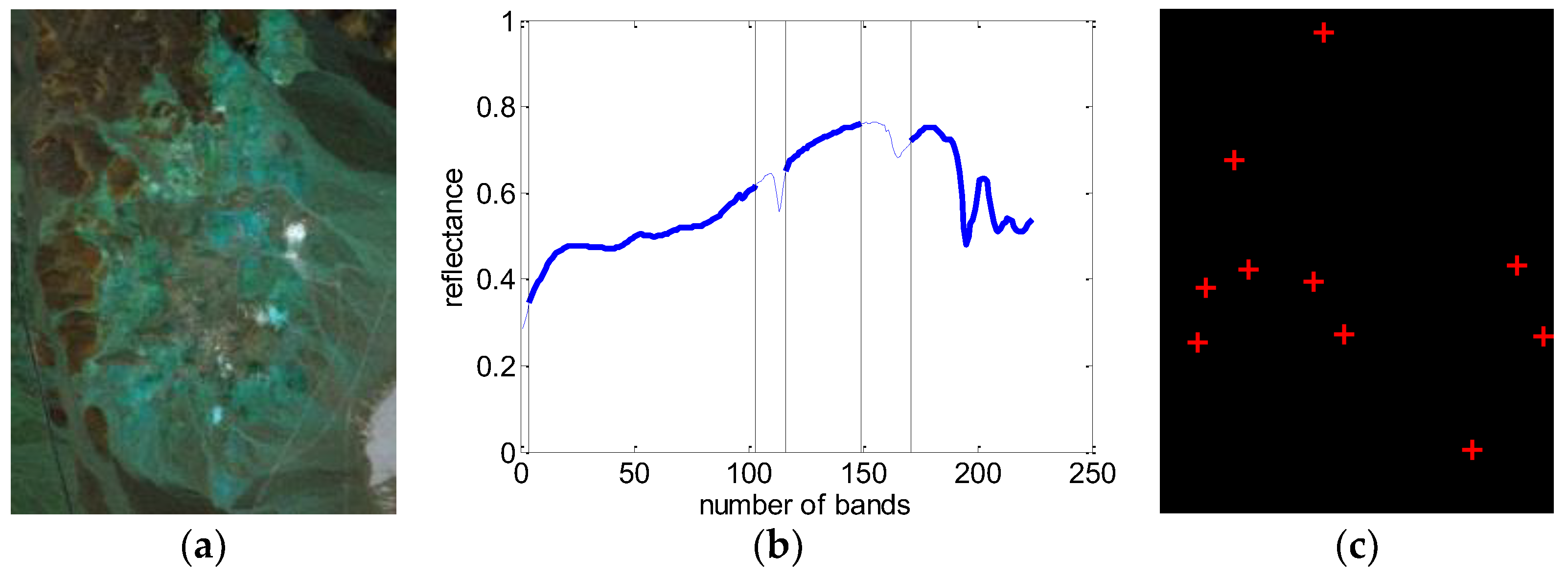
The background of the synthetic data comes from the Cuprite dataset collected by an Airborne Visible/InfraRed Imaging Spectrometer (AVIRIS) (http://www.ehu.eus/ccwintco/index.php?title=Hyperspectral_Remote_Sensing_Scenes), containing 224 bands. After removal of low-SNR and water absorption bands, 188 bands remained. A region with the size of 250 × 191 pixels, shown in Figure 1a, is selected as the background. The embedded target spectrum (shown in Figure 1b) is Muscovite_GD111 from the U.S. Geological Survey (USGS) [39] spectral set, with the same bands being removed. Five targets with size 1 × 1 and five targets with size 2 × 2 (shown in Figure 1c) are randomly embedded in the background. Due to the low spatial resolution of HSI, mixed pixels widely exist in practice. Linear mixing model (LMM) [40] is a simple but physically meaningful model which is very popular and useful in describing the mixed pixels. Based on the LMM, a synthetic target spectrum $z$ is generated. It is mixed by a desired target spectrum $t$ and a background pixel spectrum $b$ according to a random abundance fraction $f$ between 0 and 1:

$$z=f\cdot t+(1-f)\cdot b$$

(19)

If the abundance fraction $f$ is large enough, the synthetic pixel $z$ becomes more similar to the target $t$. In this case, the target can be detected easily. However, $z$ may be separated into the background when $f$ is very small, which may result in the failure of detection. After that, 30 dB Gaussian white noise is added into the synthetic data.

The detection accuracy is evaluated by receiver operating characteristic (ROC) curves [41] and their areas under the curves (AUCs). Based on the ground truth, the ROC curves describe the varying relationship of detection probability $P_d$ and false alarm rate $P_f$, which provide an unbiased quantitative and threshold-free performance comparison of the different detectors. ROC curves have been widely used as a performance evaluation tool in TD applications. $P_d$ and $P_f$ are defined as follows:

$$P_d=\frac{N_d}{N_t}\mathrm{and}{P}_f=\frac{N_f}{N_{all}}$$

(20)

where $N_d$ represents the number of detected target pixels under a certain threshold, $N_t$ represents the number of target pixels in the image, $N_f$ represents the number of background pixels mistaken as targets, and $N_{all}$ represents the total number of pixels in the image.

1) Parameters Analysis

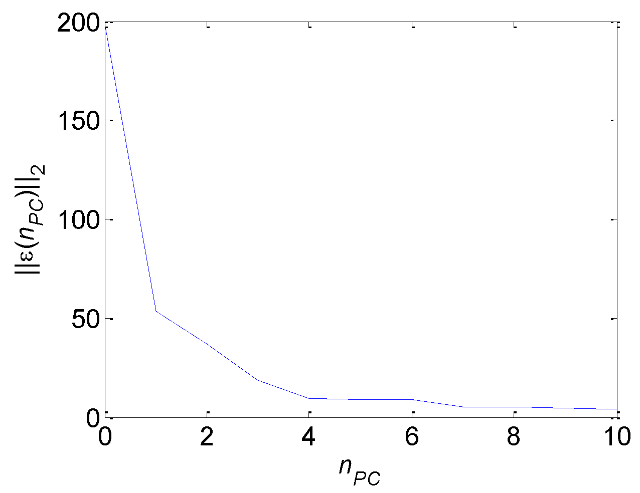
First, the impact of the parameters on TD is analyzed using the synthetic data shown in Figure 1. The curve in Figure 2 shows how ${\Vert \mathcal{E}(n_{PC})\Vert }_2$ varies with $n_{PC}$ according to Equation (18). It can be observed that the energy of the residual part changes slowly after the 4th PC. Moreover, three, four, and five PCs are used to obtain the residual part for the TD, respectively. The experimental results are shown in Figure 3 and

Table 2. AUCs of ROC curves for TPCA-based TD with different numbers of PCs.

TD Algorithm	Number of PCs
	3	4	5
CEM	0.9682	0.9945	0.9862
ACE	0.9225	0.9602	0.9264
AMF	0.9719	0.9891	0.9714

, indicating that not only is the criterion in Equation (18) effective, but the TPCA-based preprocessing method is also robust to the number of PCs. The bold in all the tables in this paper denotes the highest AUCs.

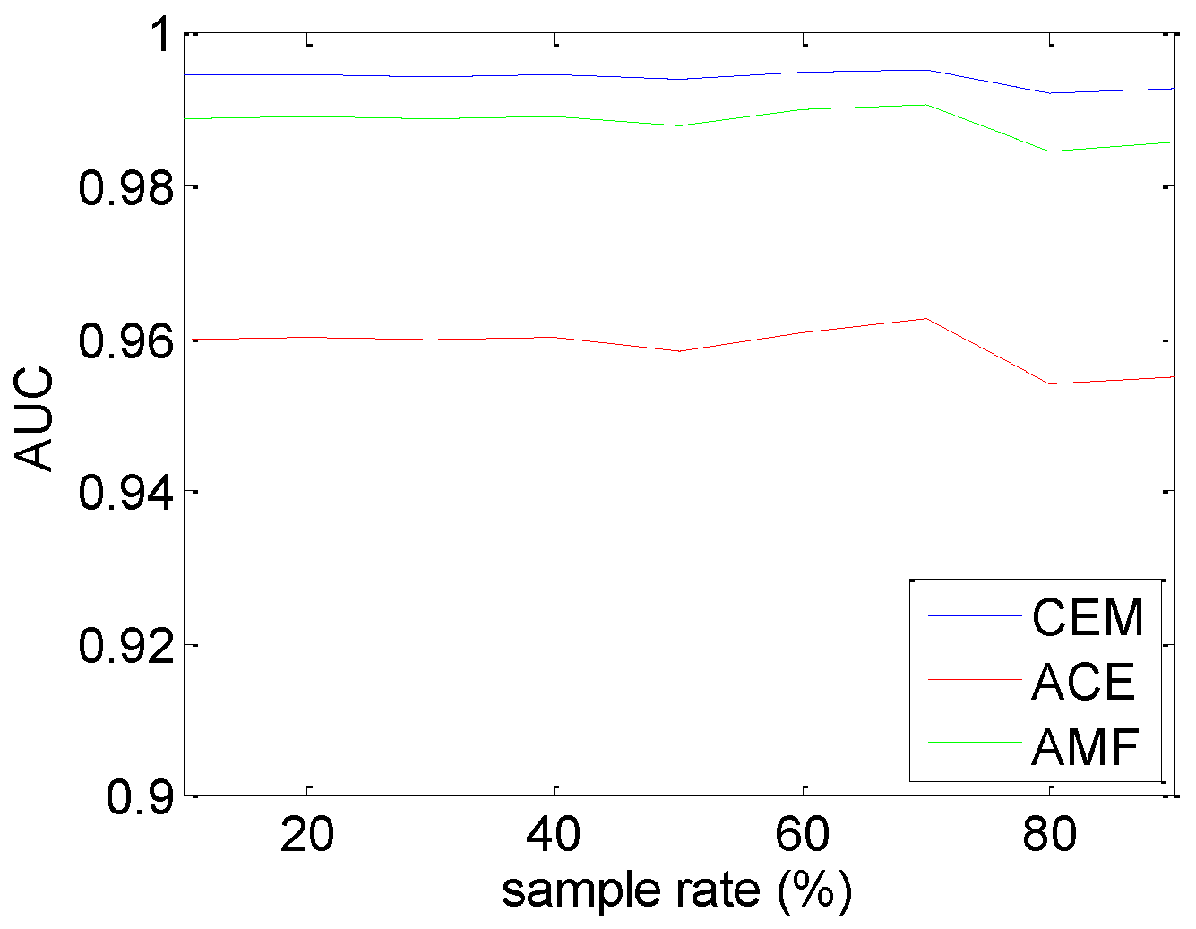
Second, the impact of the sample rate on the TD results is investigated when 10–90% of the pixels of the dataset are tensorized as the training samples. The AUCs obtained for the ROC curves are shown in Figure 4. It indicates that the rate of training samples has no obvious effect on the detection results. Therefore, we select 40% of the pixels in the image as the training samples for the following experiments.

Third, the impact of the size of the tensorization neighborhood is studied. Different neighborhood sizes are selected, and the number of PCs is set as 4 and the sample rate is 40%. The ROC curves and the running times of the TPCA algorithm are displayed in Figure 5 and

Table 3. AUCS and running time with different neighborhood sizes.

TD Algorithm	Size of Neighborhood
	2 × 2	3 × 3	4 × 4	5 × 5
CEM	0.8793	0.9945	0.9935	0.9891
ACE	0.8755	0.9602	0.9549	0.9376
AMF	0.8976	0.9891	0.9873	0.9779
Running time (s)	136.3433	227.4857	337.1790	499.2109

, respectively. It can be observed that the best detection results are obtained when the size of the neighborhood is 3 × 3. This is because the size 2 × 2 fails to contain enough spatial information, while the size larger than 3 × 3 comprises superfluous spatial information. Additionally, a TPCA with a neighborhood size larger than 3 × 3 is more time-consuming.

2) Quantitative Evaluation of TD Results

Finally, the performances of the feature extraction algorithms PCA and Tucker decomposition for TD, and the TD results obtained using the original imagery (noted as original) are compared in the following experiments. The numbers of PCs in the PCA and Tucker decomposition’s spectral domain are set to be the same as TPCA. According to Figure 6, the numbers of PCs in the Tucker decomposition’s spatial dimensions (noted as the PC number of SD1 and the PC number of SD2, respectively) are both set to five, corresponding to the best results. The sample rate of the PCA is consistent with the TPCA’s. Here, the number of PCs is set as 4, the sample rate is equal to 40%, and the spatial neighborhood size is 3 × 3 for TPCA.

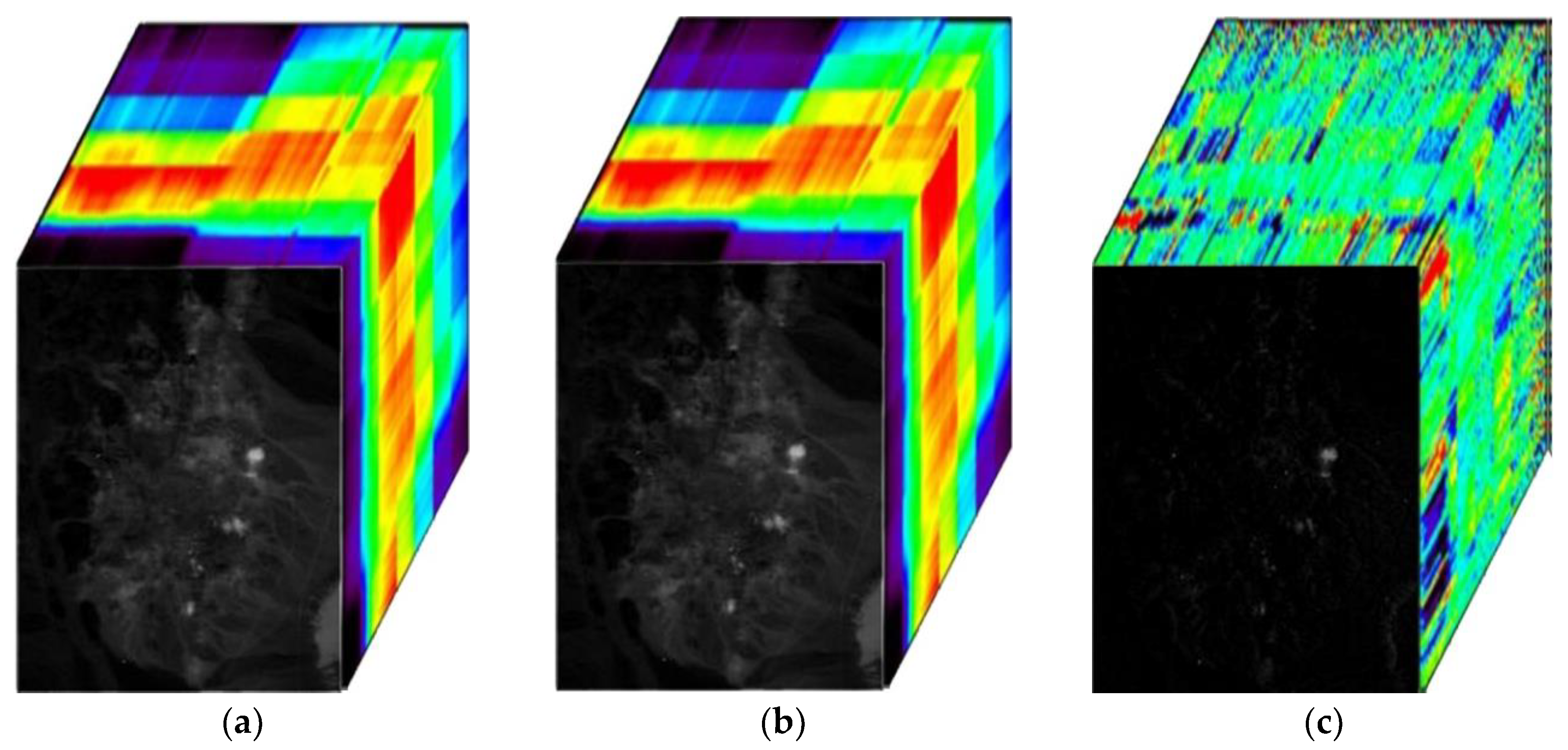
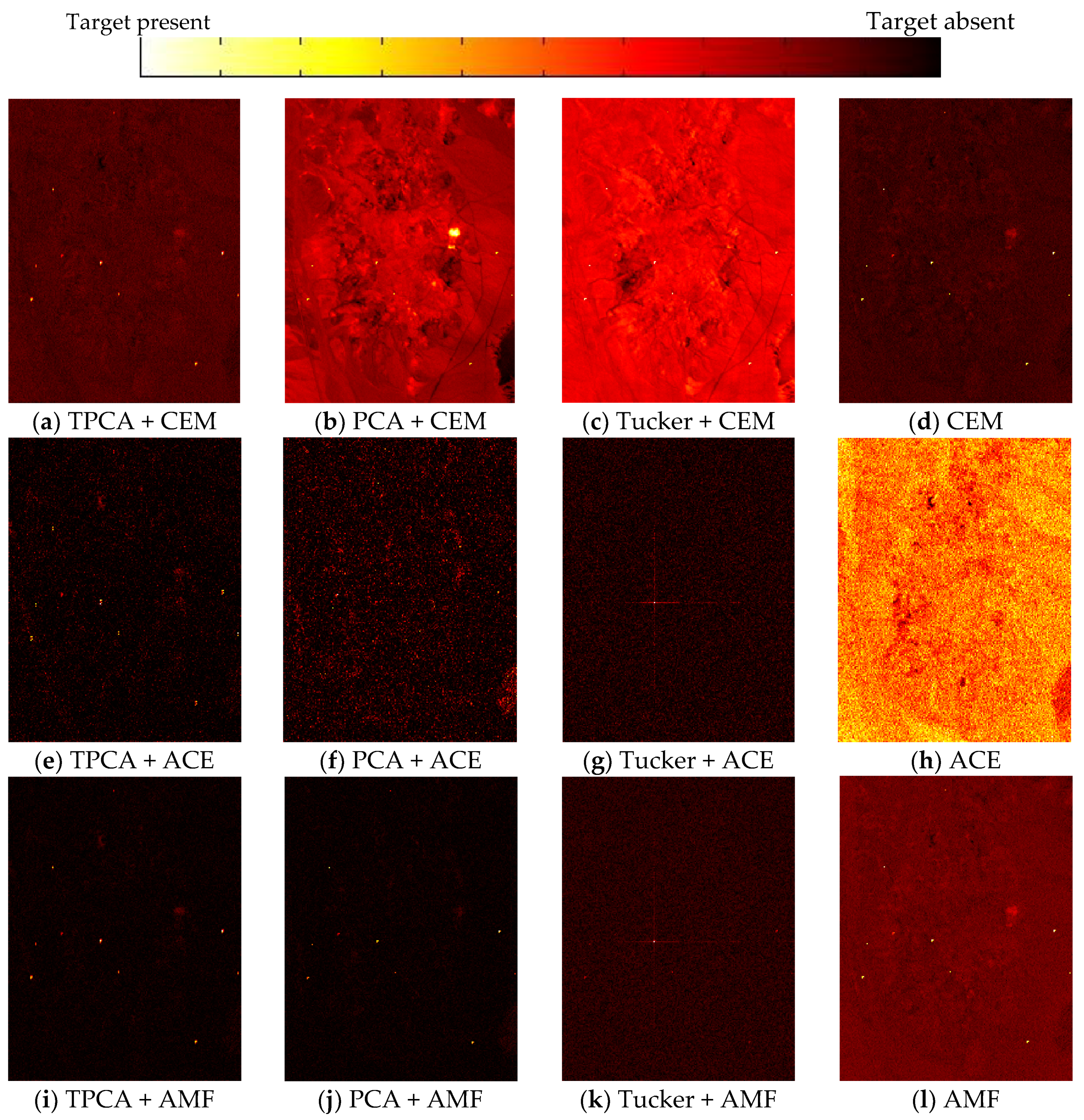
Figure 7 indicates, for the original imagery $\mathcal{X}$ of the synthetic data, its PC part $\mathcal{X}\text{'}$ and residual part $\mathcal{E}$. The result clearly reveals that, with our TPCA method, the background mostly appears in the PC part and can be removed, while the targets are well preserved in the residual part. Using the preprocessed results, TD is performed for the residual part by CEM [8], ACE [9] and AMF [10], individually. It can be observed from the detection results in Figure 8 and Figure 9 that, among the TD algorithms combining various feature extraction methods with CEM, ACE and AMF, the TPCA preprocessing method has the best TD results.

Moreover, to further study the stability of the proposed algorithm, the experiments are repeated 20 times with randomly generated target pixels’ locations and embedded abundances. The AUCs are shown in

Table 4. AUCs of ROC curves for TD for synthetic data with different feature extraction methods repeated 20 times.

TD Algorithm	Feature Extraction Method
	Original	PCA	Tucker	TPCA
CEM	0.8951$\pm$0.0301	0.9225 $\pm$ 0.0221	0.9005$\pm$0.0187	0.9995$\pm$0.0011
ACE	0.2416$\pm$0.0938	0.8987$\pm$0.0227	0.8879$\pm$0.0395	0.9845$\pm$0.0073
AMF	0.8935$\pm$0.0304	0.9195$\pm$0.0239	0.9031$\pm$0.0259	0.9991$\pm$0.0022

. The experimental results show that the TPCA-based TD algorithm provides the best and the most stable detection results. This is because the proposed method can take advantage of TPCA to reflect HSI’s physical property compared with that of other preprocessing approaches.

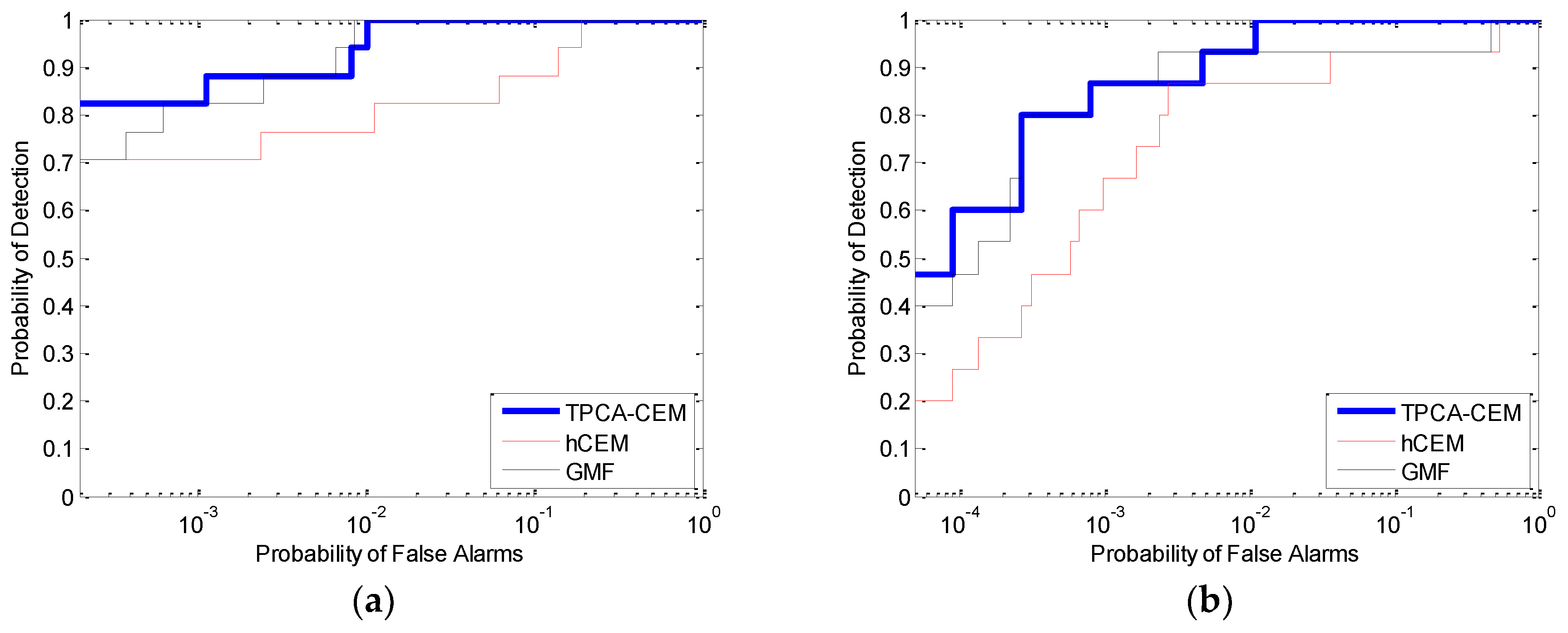
By simply combining our TPCA-based preprocessing method with the traditional TD algorithm, a novel target detector can be obtained. For instance, our TPCA-based method can be incorporated with CEM [8] to form a TPCA + CEM detector. The experiments are repeated 20 times with randomly generated target pixel locations and embedded abundances. The experimental results shown in

Table 5. AUCs and running times for TD on synthetic datasets with different TD algorithms repeated 20 times.

TD Algorithm	TPCA + CEM	hCEM	GMF
AUC	0.9995$\pm$0.0011	0.9196$\pm$0.0249	0.9000$\pm$0.0258
Running Time (s)	227.8652$\pm$0.8777	2.2876$\pm$0.0449	2.5866$\pm$0.0548

indicate that the combination TPCA + CEM has superiority in TD accuracy and stability compared with that of state-of-the-art detection algorithms that are designed to suppress background interference such as hierarchical CEM (hCEM) [14] and geometric matched filter (GMF) [15,16].

4.2. Real Data Experiments

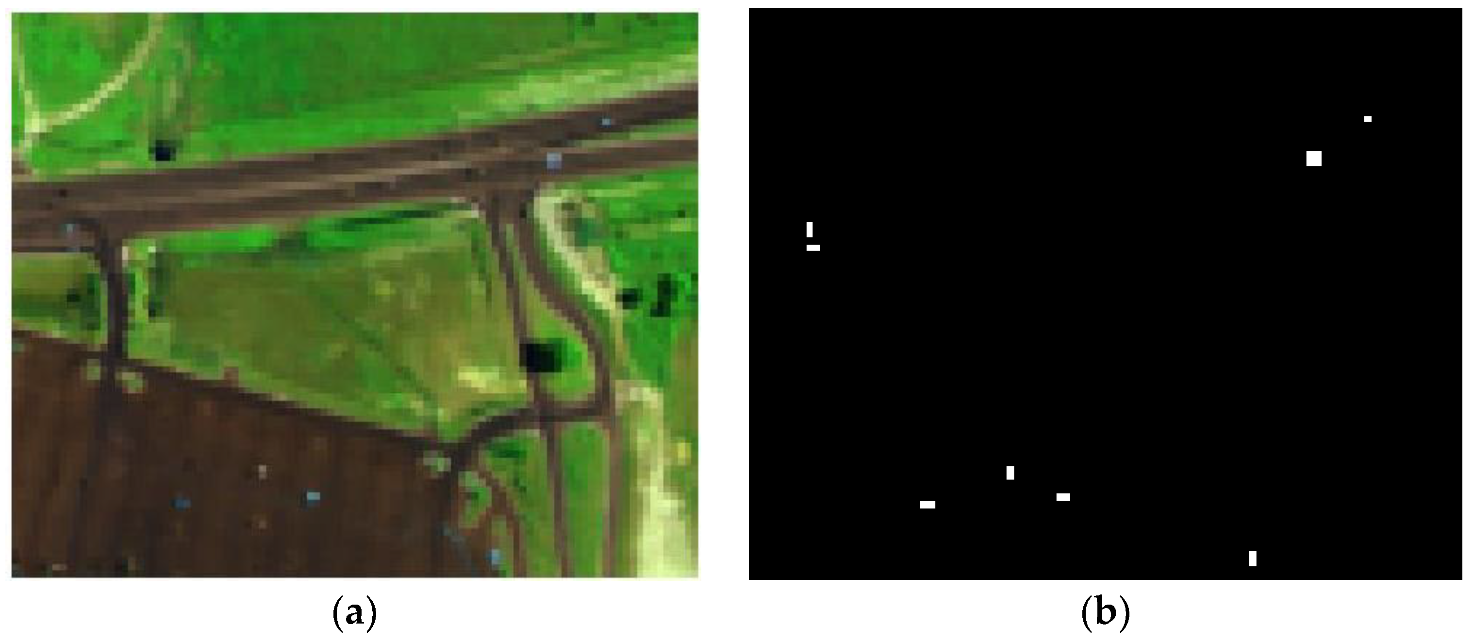
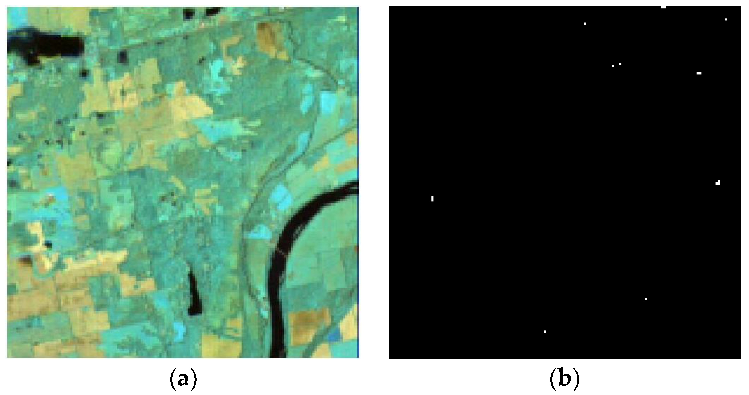
Two publicly available hyperspectral datasets are employed in the real data experiments. The first dataset was collected by a HYperspectral Digital Imagery Collection Experiment (HYDICE) sensor. It contains 210 bands, and 188 bands are used after the removal of the low SNR and water absorption bands. An interest region of 80 × 100 pixels is used. The second hyperspectral dataset was collected by Hyperion sensor, and has 242 bands. After discarding the low SNR and water absorption bands, 155 bands remained. The pseudocolor images and ground truths of the two real datasets are shown in Figure 10 and Figure 11, respectively. The number of PCs is selected according to Equation (18).

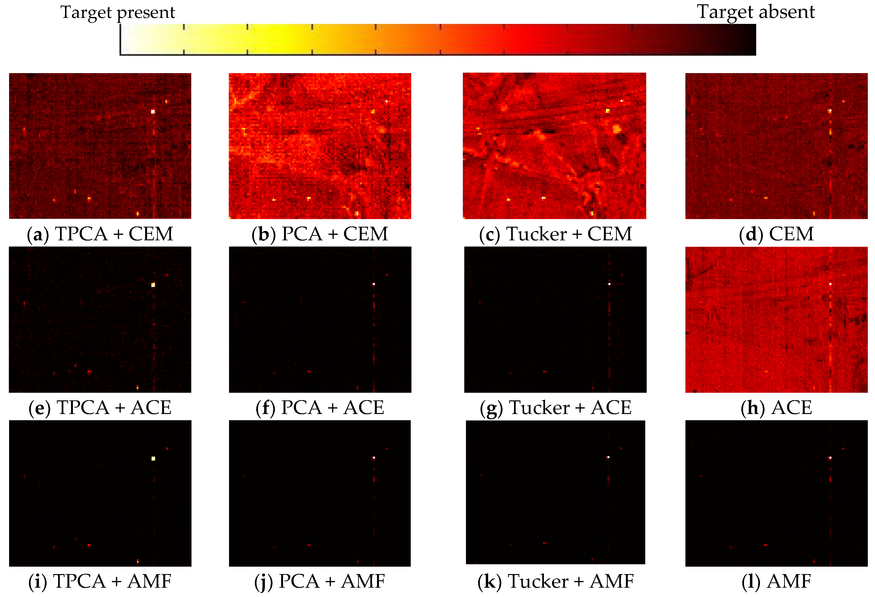
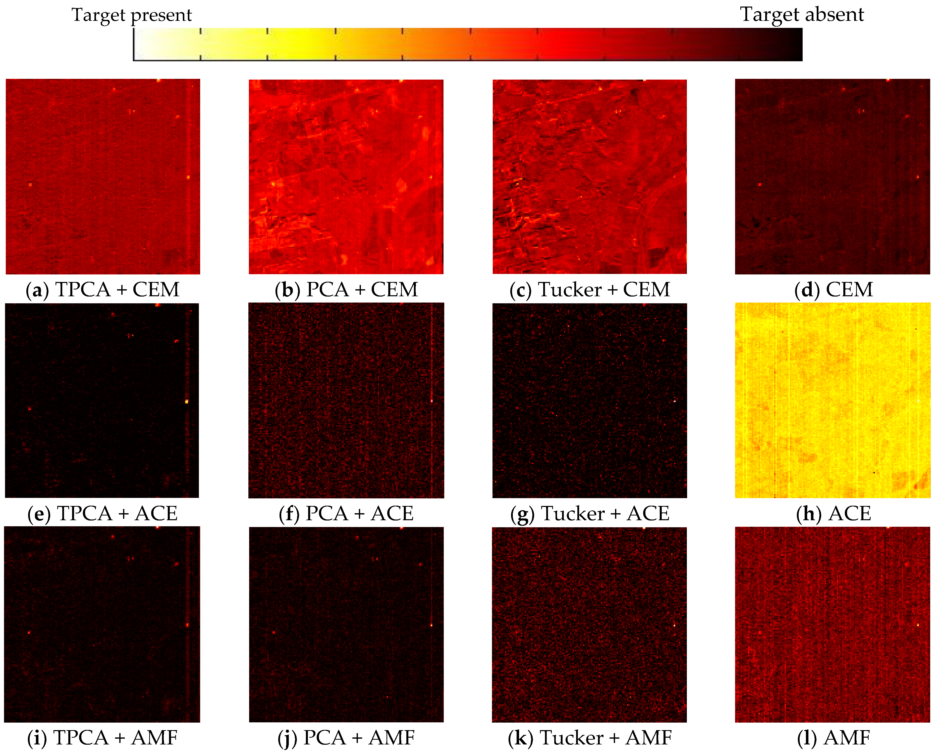
TD is also operated by CEM, ACE, and AMF using the original imagery and the residual parts of PCA, Tucker decomposition, and TPCA, respectively. The detection results are shown in Figure 12 and Figure 13. The ROC curves are presented in Figure 14 and Figure 15. The AUCs are displayed in

Table 6. AUCs and running time for the TD of synthetic datasets with different TD algorithms.

Dataset	TD Algorithm	Feature Extraction Method
		Original	PCA	Tucker	TPCA
HYDICE	CEM	0.9847	0.9671	0.9916	0.9988
	ACE	0.8079	0.9041	0.9371	0.9956
	AMF	0.9847	0.9325	0.9579	0.9986
Hyperion	CEM	0.9709	0.9918	0.9281	0.9988
	ACE	0.7053	0.8524	0.9079	0.9965
	AMF	0.9643	0.9492	0.9165	0.9824

. Similar to the experimental results of the synthetic data, the experimental results of the real data also reveal that the proposed method performs better than other methods do for both the HYDICE and Hyperion datasets. Similar to the operations for synthetic data, the TPCA-based preprocessing method is integrated with traditional detectors, such as CEM. The ROC curves demonstrated in Figure 16 and the AUCs and running time presented in

Table 7. AUCs and running time for the TD of real datasets with different TD algorithms.

Dataset	TD Algorithm	AUC	Running Time (s)
HYDICE	TPCA + CEM	0.9988	55.2074
	hCEM	0.9759	0.6258
	GMF	0.9949	0.5445
Hyperion	TPCA + CEM	0.9988	119.4458
	hCEM	0.9614	0.9226
	GMF	0.9684	1.0567

prove that our method outperforms the state-of-the-art TD algorithms in terms of TD accuracy but has a higher time cost. This result is because the computational complexity of tensor calculations is high, which is induced by retaining the spatial relationships in numerous local patches of images. In this sense, the acceleration of this procedure can be a very meaningful goal in practical applications.

5. Discussion

5.1. Experimental Results Analysis

The detection results shown in Section 4 indicate that our TPCA-based preprocessing method has a remarkable background energy suppression property. Parameter analysis experiments operated on synthetic data not only demonstrate that the employed number of PCs selecting criterion in Equation (18) is valid but also provide the best parameters for later experiments: the TPCA sample rate is 40% and size of the neighborhood is 3 × 3. It implies that the simplicity of parameter selection in our TPCA-based algorithm can be proven.

Figure 7 describes the PC part and the residual part. The PC part is mostly similar to the synthetic data, and the targets lie in the residual part. This result demonstrates that our TPCA-based preprocessing method can leave most of the background information in the PC part, while targets are preserved in the residual part. The detection results shown in Figure 8 indicate the effectiveness of different preprocessing methods in various TD methods. Compared with that of other methods, fewer background pixels are detected as targets by the proposed TPCA-based preprocessing method. It can be explained that less background energy is remaining in the residual part of our method than that in others. Although Tucker decomposition is also good at background suppression, the target information is lacking in its residual part. The ROC curves in Figure 9 give support to the visualized results in Figure 8. The higher detection probability and lower false alarm rate signifies more target preservation and background removal. After repeating the experiments 20 times to randomly generate various synthetic data, the results shown in Table 4 manifest the stability of our TPCA-based algorithm. Furthermore, our preprocessing method not only improves the performances of traditional target detectors but also constructs new compositional detectors by simply combining the TPCA method with traditional detectors. The results in Table 5 prove that the effectiveness of the TPCA + CEM detector is even better than the state-of-the-art hCEM and GMF detectors aimed at background suppression.

Adopting the parameters selecting criterion mentioned above, detections are carried out in two real hyperspectral datasets, HYDICE data and Hyperion data. According to the detection results shown in Figure 12 and Figure 13, similar conclusions to the synthetic data experiments can be drawn. Our TPCA-based approach has more remarkable performance in both background separation and target preservation. Compared with PCA, Tucker decomposition and original imagery, the targets are more conspicuous and the results are clearer with TPCA-based preprocessing. A convincing instance can be derived from the performance of the ACE detector in the Hyperion dataset. Targets are difficult to identify among false alarm pixels in the original image and Tucker decomposition detection results, and few targets are discerned in the PCA detection result. However, the ACE detector performs well in the TPCA residual part. The ROC curves shown in Figure 14 and Figure 15, as well as AUCs listed in Table 6 also confirm the outperformance of our method. Figure 16 and Table 7 indicate that the TPCA + CEM combination detector rivals the state-of-the-art algorithms designed for background suppression, and the former behaves even better.

In brief, experiments on both synthetic data and real data reveal the superiority of our TPCA-based preprocessing method in terms of detection accuracy over that of PCA and Tucker decomposition. Furthermore, regarding the HSI target detector, by combining TPCA with traditional TD methods such as CEM, it can outperform the state-of-the-art algorithms aimed at background suppression.

5.2. Advantages and Limitations

From the previous discussions, the advantages of the TPCA-based preprocessing method are briefly summarized as follows:

• The employment of the TPCA-based method can take advantage of information of both the one spectral dimension and two spatial dimensions simultaneously, which is consistent with the HSI physical property. Higher detection accuracy and stability are obtained using our TPCA-based method than that with traditional algorithms and the state-of-the-art algorithms.
• Very few parameters must be determined manually. According to the discussion in Section 4, the number of PCs can be automatically calculated by Equation (18), and, further, our method is robust to different sample rates.
• Since our TPCA-based preprocessing method can be combined with any traditional TD method (such as CEM), it should provide great flexibility for practical use.

However, our method has an inevitably high time cost, which is its main limitation. Acceleration strategies will be investigated in our future work, for instance, the adoption of more effective strategies to construct the tensor computation and the use of parallel computation and GPU.

6. Conclusions

In this paper, a novel TPCA-based preprocessing method for hyperspectral TD is proposed to alleviate background interference. The proposed method decomposes a HSI into the sum of a PC part and a residual part via TPCA. Because the target is scarce in HSI, the residual part can be effectively utilized to perform TD and greatly reduce the background interference. Compared with other preprocessing methods, the TPCA-based method performs better in revealing the HSI physical property. The experimental results on both the synthetic and real hyperspectral datasets showed that the accuracy of the traditional TD methods can be greatly improved by using the proposed preprocessing method. Moreover, detection approaches that combine our TPCA-based preprocessing method with traditional TD methods outperformed the state-of-the-art algorithms aimed at background suppression.

However, there are some issues to be addressed in further research. The high computational complexity associated with tensor methods should be reduced for practical use. A more effective strategy to construct the tensor computation will be studied. Furthermore, we will focus on more efficient methods, such as parallel processing or GPU computing, to accelerate the computation.

References

1. Matteoli, S.; Diani, M.; Theiler, J. An overview of background modeling for detection of targets and anomalies in hyperspectral remotely sensed imagery. IEEE J. Sel. Top. Appl. Earth Observ. Remote Sens. 2014, 7, 2317–2336. [Google Scholar] [CrossRef]
2. Plaza, A.; Bioucas-Dias, J.M.; Simic, A.; Blackwell, W.J. Foreword to the special issue on hyperspectral image and signal processing. IEEE J. Sel. Top. Appl. Earth Observ. Remote Sens. 2012, 5, 347–353. [Google Scholar] [CrossRef]
3. Lillesland, T.M.; Kiefer, R.W.; Chipman, J.W. Remote Sensing and Image Interpretation; John Wiley & Sons Ltd.: Hoboken, NJ, USA, 2004. [Google Scholar]
4. Grahn, H.F.; Gelado, P. Techniques and Applications of Hyperspectral Image Analysis; John Wiley & Sons Ltd.: Hoboken, NJ, USA, 2007. [Google Scholar]
5. Hakkenberg, C.R.; Peet, R.K.; Urban, D.L.; Song, C. Modeling plant composition as community continua in a forest landscape with LiDAR and hyperspectral remote sensing. Ecol. Appl. 2018, 28, 177–190. [Google Scholar] [CrossRef] [PubMed]
6. Manolakis, D.; Truslow, E.; Pieper, M.; Cooley, T.; Brueggeman, M. Detection algorithms in hyperspectral imaging systems: An overview of practical algorithms. IEEE Signal Process. Mag. 2014, 31, 24–33. [Google Scholar] [CrossRef]
7. Nasrabadi, N.M. Hyperspectral target detection: An overview of current and future challenges. IEEE Signal Process. Mag. 2014, 31, 34–44. [Google Scholar] [CrossRef]
8. Harsanyi, J.C. Detection and Classification of Subpixel Spectral Signatures in Hyperspectral Image Sequences. Ph.D. Thesis, University of Maryland Baltimore County, Baltimore, MD, USA, 1993. [Google Scholar]
9. Kraut, S.; Scharf, L.; McWhorter, L. Adaptive sub-space detectors. IEEE Trans. Signal Process. 2001, 49, 1–16. [Google Scholar] [CrossRef]
10. Robey, F.C.; Fuhrmann, D.R.; Kelly, E.J.; Nitzberg, R. A CFAR adaptive matched filter detector. IEEE Trans. Aerosp. Electron. Syst. 1992, 28, 208–216. [Google Scholar] [CrossRef]
11. Chang, S.; Du, B.; Zhang, L.; Zhao, R. IBRS: An iterative background reconstruction and suppression framework for hyperspectral target detection. IEEE J. Sel. Top. Appl. Earth Observ. Remote Sens. 2017, 10, 3406–3417. [Google Scholar] [CrossRef]
12. Niu, Y.; Wang, B. Extracting target spectrum for hyperspectral target detection: An adaptive weighted learning method using a self-completed background dictionary. IEEE Trans. Geosci. Remote Sens. 2017, 55, 1604–1617. [Google Scholar] [CrossRef]
13. Yang, S.; Shi, Z. Hyperspectral image target detection improvement based on total variation. IEEE Trans. Image Process. 2016, 25, 2249–2258. [Google Scholar] [CrossRef] [PubMed]
14. Zou, Z.; Shi, Z. Hierarchical suppression method for hyperspectral target detection. IEEE Trans. Geosci. Remote Sens. 2016, 54, 330–342. [Google Scholar] [CrossRef]
15. Manolakis, D.; Lockwood, R.; Cooley, T.; Jacobson, J. Is there a best hyperspectral detection algorithm? In Proceedings of the SPIE Defense, Security, and Sensing, Orlando, FL, USA, 13–17 April 2009. [Google Scholar]
16. Akhter, M.A.; Heylen, R.; Scheunders, P. A geometric matched filter for hyperspectral target detection and partial unmixing. IEEE Geosci. Remote Sens. Lett. 2015, 12, 661–665. [Google Scholar] [CrossRef]
17. Oliver, N.M.; Rosario, B.; Pentland, A.P. A Bayesian computer vision system for modeling human interactions. IEEE Trans. Patt. Analy. Mach. Intell. 2000, 22, 831–843. [Google Scholar] [CrossRef] [Green Version]
18. Boukhechba, K.; Wu, H.; Bazine, R. DCT based preprocessing approach for ICA in hyperspectral data analysis. Sensors 2018, 18, 1138. [Google Scholar] [CrossRef] [PubMed]
19. Fakiris, E.; Papatheodorou, G.; Geraga, M.; Ferentinos, G. An automatic target detection algorithm for swath sonar backscatter imagery, using image texture and independent component analysis. Remote Sens. 2016, 8, 373. [Google Scholar] [CrossRef]
20. Smith, W.S. Principles and Applications of Tensor Analysis; The Bobbs-Merril Company: Indianapolis, IN, USA, 1963. [Google Scholar]
21. Silverman, R.A.; Borisenko, A.I.; Tarapov, I.E. Vector and Tensor Analysis with Applications; Prentice Hall Press: Upper Saddle River, NJ, USA, 1968. [Google Scholar]
22. Kolda, T.G.; Bader, B.W. Tensor decompositions and applications. SIAM Rev. 2009, 51, 455–500. [Google Scholar] [CrossRef]
23. Zhang, X.; Wen, G.; Dai, W. A tensor decomposition-based anomaly detection algorithm for hyperspectral image. IEEE Trans. Geosci. Remote Sens. 2016, 54, 5801–5820. [Google Scholar] [CrossRef]
24. Veganzones, M.A.; Cohen, J.E.; Cabral Farias, R.; Chanussot, J.; Comon, P. Nonnegative tensor CP decomposition of hyperspectral data. IEEE Trans. Geosci. Remote Sens. 2016, 54, 2577–2588. [Google Scholar] [CrossRef]
25. Zhang, K.; Wang, M.; Yang, S.; Jiao, L. Spatial–spectral-graph-regularized low-rank tensor decomposition for multispectral and hyperspectral image fusion. IEEE J. Sel. Top. Appl. Earth Observ. Remote Sens. 2018, 11, 1030–1040. [Google Scholar] [CrossRef]
26. Liu, Y.; Gao, G.; Gu, Y. Tensor matched subspace detector for hyperspectral target detection. IEEE Trans. Geosci. Remote Sens. 2017, 55, 1967–1974. [Google Scholar] [CrossRef]
27. Ren, Y.; Liao, L.; Maybank, S.J.; Zhang, Y.; Liu, X. Hyperspectral image spectral-spatial feature extraction via tensor principal component analysis. IEEE Geosci. Remote Sens. Lett. 2017, 14, 1431–1435. [Google Scholar] [CrossRef]
28. Golub, G.H.; Loan, C.F.V. Matrix Computations; John Hopkins University Press: Baltimore, MD, USA, 1983. [Google Scholar]
29. Proakis, J.G.; Manolakis, D.G. Digital Signal Processing: Principles, Algorithms and Applications; Prentice Hall Press: Upper Saddle River, NJ, USA, 1996. [Google Scholar]
30. Oppenheim, A.V.; Schafer, R.W. Discrete-Time Signal Processing; Prentice Hall Press: Upper Saddle River, NJ, USA, 2009. [Google Scholar]
31. Keshava, N.; Mustard, J.F. Spectral unmixing. IEEE Signal Process. Mag. 2002, 19, 44–57. [Google Scholar] [CrossRef]
32. Feller, W. An Introduction to Probability Theory and Its Applications; Wiley: Hoboken, NJ, USA, 1971. [Google Scholar]
33. Lehmann, E.L. Testing Statistical Hypotheses; John Wiley & Sons Ltd.: Hoboken, NJ, USA, 1959. [Google Scholar]
34. Kilmer, M.E.; Martin, C.D. Factorization strategies for third-order tensors. Linear Algebra Appl. 2011, 435, 641–658. [Google Scholar] [CrossRef]
35. Braman, K. Third-order tensors as linear operators on a space of matrices. Linear Algebra Appl. 2010, 433, 1241–1253. [Google Scholar] [CrossRef]
36. Kilmer, M.E.; Braman, K.; Hao, N.; Hoover, R.C. Third-order tensors as operators on matrices: A theoretical and computational framework with applications in imaging. SIAM J. Matrix Anal. Appl. 2013, 34, 148–172. [Google Scholar] [CrossRef]
37. Cooley, J.W.; Tukey, J.W. An algorithm for the machine calculation of complex Fourier series. Math. Comput. 1965, 19, 297–301. [Google Scholar] [CrossRef]
38. Horn, R.A.; Johnson, C.R. Matrix Analysis; Cambridge University Press: Cambridge, UK, 1990. [Google Scholar]
39. Clark, R.N.; Swayze, G.A.; Gallagher, A.J.; King, T.V.V.; Calvin, WM. The U.S. Geological Survey Digital Spectral Library: Version 1: 0.2 to 3.0 μm; Open File Report; U.S. Geological Survey: Denver, CO, USA, 1993.
40. Stefanou, M.S.; Kerekes, J.P. A method for assessing spectral image utility. IEEE Trans. Geosci. Remote Sens. 2009, 47, 1698–1706. [Google Scholar] [CrossRef]
41. Kerekes, J. Receiver operating characteristic curve confidence intervals and regions. IEEE Geosci. Remote Sens. Lett. 2008, 5, 251–255. [Google Scholar] [CrossRef]
Figure 1. Synthetic data: (a) pseudocolor image (Bands 160, 100, and 40 for RGB); (b) embedded target spectrum; and (c) ground truth.
Remotesensing 10 01033 g001
Figure 2. The curve of E ( n P C ) 2 varying with n P C .
Remotesensing 10 01033 g002
Figure 3. ROC curves with different PC numbers: (a) CEM; (b) ACE; and (c) AMF.
Remotesensing 10 01033 g003
Figure 4. AUCs with different sample rates.
Remotesensing 10 01033 g004
Figure 5. ROC curves obtained by using different sizes of neighborhoods: (a) CEM; (b) ACE; and (c) AMF.
Remotesensing 10 01033 g005
Figure 6. AUCs of Tucker decomposition-based TD with different numbers of spatial PCs: (a) CEM; (b) ACE; and (c) AMF.
Remotesensing 10 01033 g006
Figure 7. The synthetic dataset: (a) original imagery X ; (b) PC part X ' ; and (c) residual part E .
Remotesensing 10 01033 g007
Figure 8. Detection results of the synthetic dataset with different feature extraction methods and traditional TD methods.
Remotesensing 10 01033 g008
Figure 9. ROC curves with different feature extraction methods: (a) CEM; (b) ACE; and (c) AMF.
Remotesensing 10 01033 g009
Figure 10. HYDICE data: (a) pseudocolor image (Bands 160, 100, and 40 for RGB); and (b) ground truth.
Remotesensing 10 01033 g010
Figure 11. Hyperion data: (a) pseudocolor image (Bands 120, 80, and 40 for RGB); and (b) ground truth.
Remotesensing 10 01033 g011
Figure 12. Detection results of the HYDICE dataset with different feature extraction methods and traditional TD methods.
Remotesensing 10 01033 g012
Figure 13. Detection results of the Hyperion dataset with different feature extraction methods and traditional TD methods.
Remotesensing 10 01033 g013
Figure 14. ROC curves with different feature extraction methods for HYDICE data: (a) CEM; (b) ACE; and (c) AMF.
Remotesensing 10 01033 g014
Figure 15. ROC curves with different feature extraction methods for Hyperion data: (a) CEM; (b) ACE; and (c) AMF.
Remotesensing 10 01033 g015
Figure 16. ROC curves with different target detection methods for the real data: (a) HYDICE; and (b) Hyperion.
Remotesensing 10 01033 g016