Inland Water Atmospheric Correction Based on Turbidity Classification Using OLCI and SLSTR Synergistic Observations

Abstract

Atmospheric correction is an essential prerequisite for obtaining accurate inland water color information. An inland water atmospheric correction algorithm, ACbTC (Atmospheric Correction based on Turbidity Classification), was proposed in this study by using OLCI (Ocean and Land Color Instrument) and SLSTR (Sea and Land Surface Temperature Radiometer) synergistic observations for the first time. This method includes two main steps: (1) water turbidity classification by the GRA index (GRAdient of the spectrum index); and (2) atmospheric correction by synergistic use of OLCI and SLSTR images. The algorithm was validated with 72 in situ sampling sites in Lake Erhai, Lake Hongze, and Lake Taihu, and compared with other atmospheric correction methods, i.e., C2RCC (Case 2 Regional Coast Colour processor), MUMM (Management Unit of the North Seas Mathematical Models), FLAASH (Fast Line-of-sight Atmospheric Analysis of Hypercubes), POLYMER (POLYnomial based algorithm applied to MERIS), and BPAC (Bright Pixel Atmospheric Correction). The results show that (1) the GRA index performed better than the proposed turbidity classification indices, i.e., the Diff (spectral difference index) and the Tind (turbid index), in inland lakes by using the reflectance peak at 1020 nm in clean water; (2) the synergistic use of OLCI and SLSTR performed feasibly for atmospheric correction, and the ACbTC algorithm achieved full-band average values of the mean absolute percentage error (MAPE) = 29.55%, mean relative percentage error (MRPE) = 13.98%, and the root mean square of error (RMSE) = 0.0039 sr⁻¹, which were more reliable than C2RCC, MUMM, FLAASH, POLYMER, and BPAC; and (3) the synergistic use of the 17th band (865 nm) on OLCI and the 5th band (1613 nm) on SLSTR are suitable for clean inland lakes, while both the 5th band (1613 nm) and 6th band (2250 nm) on SLSTR are advisable for the turbidity.

1. Introduction

The monitoring of inland lakes is becoming gradually more critical due to the increase of anthropogenic pressures and the effects of climate change [1,2]. Compared to in situ measurements, satellite measurements can provide synoptic observations of the water signal for the entire lake, with the advantages of high rates of temporal and spatial coverage [3,4]. However, the signals received by the satellite sensors include not only the water, which is the desired part, ultimately, but also atmospheric molecules and aerosols accounting for a significant portion [5]. Thus, the atmospheric correction, i.e., the removal of atmospheric effects, is an essential prerequisite for obtaining accurate water color information.

Many algorithms have been proposed for atmospheric correction [6,7,8,9,10,11]. The standard algorithm is the dark pixel method, which is based on the assumption that the signal of water in the near-infrared region (NIR) is zero [11,12]. This algorithm has been successfully used in the open ocean to determine the aerosol model. However, this hypothesis is invalid for turbid water, such as offshore water or inland lakes in which suspended particles and algae still have a strong signal in the NIR band [8,13]. To solve this problem, some researchers have tried to satisfy the assumption of dark pixels by subtracting the calculated water signal in the NIR [10,14,15,16,17]. However, the uncertainty of calculating the water signal in the NIR arises by this method because of the variety of the water components [18]. On the other hand, some researchers have tried to extend the band to the shortwave infrared region (SWIR) to satisfy the assumption because of the strong water absorption by SWIR [8,19]. Unfortunately, the substantially lower signal-noise ratio (SNR) values in SWIR [20,21,22] may reduce the accuracy of aerosol estimation in clean water. To overcome these shortcomings, Shi and Wang [23] promoted a method to detect water turbidity before the atmospheric correction, which has been widely used in coastal waters [18,24,25]. First, the turbid water is identified by a turbid water index; and, second, the atmospheric correction is conducted by SWIR algorithm for the turbid water, whereas the standard algorithm [11] is applied for non-turbid water. This algorithm uses different band combinations to calculate the aerosols’ reflectance for the different waters to decrease the error from the incorrect dark band assumption.

This method hypothesizes that the reflectance at NIR is close to zero in the open ocean. However, this hypothesis is invalid in inland waters even for relatively clean water [18,26]. Thus, the algorithm might not be suitable for detecting the turbidity of inland waters. In fact, the turbidity of inland water varies strongly. For example, the concentration of total suspended matter (TSM), which is considered as an essential indicator of lake turbidity [27], is approximately 1.24 mg/L in Lake Fuxian [28]. That is about 1/20 of Lake Taihu and Lake Dianchi, and 1/60 of Lake Hongze and Lake Poyang [29]. Among the inland lakes, the reflectance of the relatively clean waters such as Lake Fuxian is close to zero after 800 nm, while in some turbid waters, the reflectance is non-zero even after 1000 nm [30,31]. Therefore, it is necessary to use different correction bands to calculate the aerosol scattering based on different water types and facilitate the atmospheric corrections for inland waters.

In order to increase the available band for atmospheric correction, the combination of multiple sensors has been attempted and obtained better results than a single sensor [32]. However, the synergistic ability of different sensors is strongly related to the consistency of the radiative resolution, acquisition time, geo-location, etc., between the sensors. Additionally, the conditions will be more complicated when the sensors are on different satellites [33]. The new sensors of OLCI (21 bands in the range of 400–1020 nm) and SLSTR (six bands in the range of 555–2250 nm), which are the legacy of ENVISAT MERIS (Medium Resolution Imaging Spectrometer Instrument) and AATSR (Advanced Along Track Scanning Radiometer), respectively, are payloads on the Sentinel-3 satellite and can obtain synchronized data. Despite the fact that the sensors have an overlap of the spectrum range, the OLCI provides higher quality and finer water pixels in the visible region (VISR) to NIR, while the SLSTR expands to the SWIR, thus, the aerosol condition over the mostly turbid inland lakes can be observed [34]. Up to the present time the application of one independent sensor on Sentinel-3 has been conducted in several areas: the OLCI data has been widely used in ocean color research [22,35,36,37], while the applications of the SLSTR have been focused on the land and atmosphere [38,39]. Therefore, there is an urgent need to combine the Sentinel-3 synergistic data to improve the present algorithms by fully utilizing the advantages of the sensors.

The objective of this study is to provide a procedure for inland atmospheric correction by the synergistic use of the OLCI and SLSTR data based on water turbidity identification. First, this paper proposes an index to effectively detect the turbidity in inland waters; and, secondly, it constructs an atmospheric correction algorithm by taking advantages of the two data sources.

2. Study Area and Data

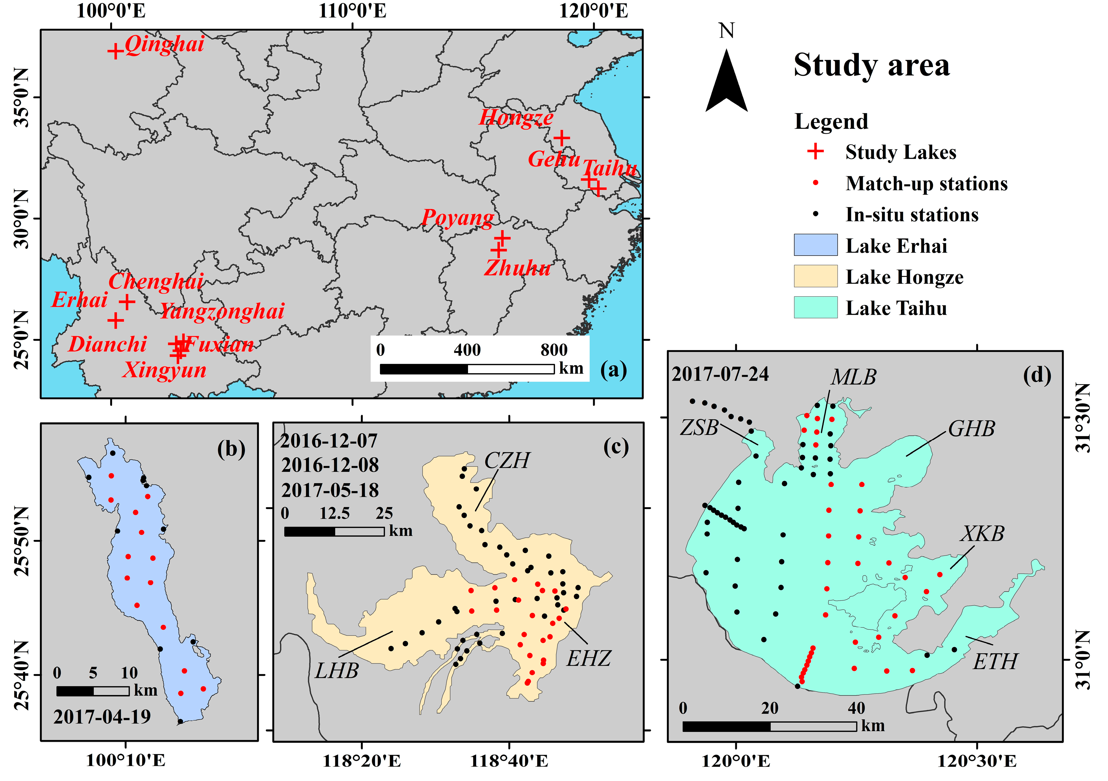
2.1. Overview of the Study Area

The 12 lakes, including plateau lakes and plains lakes (Figure 1), are surveyed in this study. Some of the plateau lakes have relatively clean water (Lake Qinghai, Lake Erhai, Lake Chenghai, Lake Yangzonghai, Lake Xingyun, and Lake Fuxian), while the other is eutrophic (Lake Dianchi) [28,40,41]. Among the plains lakes, Lake Poyang, Lake Taihu, and Lake Hongze are the first, third, and fourth largest freshwater lakes in China, respectively. Lake Taihu has suffered from eutrophication since the 1980s, and the water quality of Lake Gehu located northwest of Lake Taihu has also deteriorated in recent years [29]. Lake Poyang and Lake Hongze are dominated by suspended sediments [31,42]. While separated from Lake Poyang with a dam, Lake Zhuhu is much cleaner [43]. More detailed information about locations, elevations, and water quality parameters are provided in

Table 1. Water quality parameter mean values refer to previous studies and measured data (the turbid lakes are marked by the symbol *, respectively; E: elevation of water surface; TSM: Total Suspended Matter; Chla: Chlorophyll a; SSD: Secchi Disk Depth).

Lakes	Lon. (°E)	Lat. (°N)	E(m)	TSM(mg/L)	Chla(μg/L)	SSD(m)	Reference
Lake Hongze *	118.682	33.313	10	63.82	8.12	0.19	This study
Lake Taihu *	120.192	31.221	0	13.54	20.50	0.80	This study
Lake Gehu *	119.807	31.592	4	44.23	53.25	0.27	[29]
Lake Poyang *	116.216	29.180	10	49.88	10.42	0.65	[29]
Lake Dianchi *	102.701	24.824	1900	36.09	91.40	0.29	This study
Lake Erhai	100.190	25.785	1997	3.97	11.73	1.78	This study
Lake Chenghai	100.665	26.549	1506	7.80	0.72	1.6	[41]
Lake Fuxian	102.890	24.528	1920	1.24	1.56	5.57	[28]
Lake Xingyun	102.775	24.328	1888	-	14.5	-	[44]
Lake Yangzonghai	103.002	24.914	1930	2.07	1.10	2.40	[41]
Lake Qinghai	100.194	36.897	3200	2.28	0.857	3.18	[40]
Lake Zhuhu	116.150	29.134	13	-	7.76	1.00	[43]

.

2.2. Data and Processing

2.2.1. Image and Preprocessing

Nine full-resolution (300 m) OLCI images (OLCI Level 1B, the Instrument Processing Facility (IPF) version is 6.07) and nine corresponding full-resolution (500 m) SLSTR images (SLSTR Level 1B, the IPF version is 6.14) were acquired from the ESA (European Space Agency) data hub (https://scihub.copernicus.eu/) (see

Table 2. List of the image data used in this study. The satellite-synchronous in situ sampling measurements were observed in Lake Taihu, Lake Hongze, and Lake Erhai are in bold font.

Region	Date (ISO8601)	Sensing Time (UTC)	In-Situ Number (n = 72)
Lake Taihu Lake Gehu	24 July 2017	01:50	35
	24 July 2017	01:53
Lake Hongze	7 December 2016	02:27	8
	8 December 2016	02:01	8
	18 May 2017	02:27	7
Lake Erhai Lake Chenghai	19 April 2017	03:23	14
Lake Dianchi Lake Fuxian Lake Yangzonghai Lake Xingyun	14 November 2017	03:01	-
Lake Qinghai	12 July 2017	03:39	-
Lake Poyang Lake Zhuhu	31 October 2017	02:24	-

* The product types of images in this study are OL_1_EFR and SL_1_RBT of OLCI and SLSTR, respectively.

for details). The image pre-processing, including image reading, sub-setting, collocation, re-projecting, and radiance to reflectance transferring were performed using SNAP 6.0 (Sentinel Application Platform, http://step.esa.int /main/toolboxes/snap/), which is the toolbox designed to process and analyze the Sentinel series images. Specifically, the Sentinel-3 products were read with per-pixel geo-codings instead of using tie-points, and their vicarious calibration coefficients were set as the default (1.00 for each band) in this study. To match with available OLCI and SLSTR observations, all data were resampled to a 300 m pixel size and were converted to Universal Transverse Mercator (UTM) projection. Then, the 18 top-of-atmosphere (TOA) reflectance bands were extracted from the OLCI images of which 761.25, 764.375, 767.5, 900, and 940 nm were excluded to avoid atmospheric absorption [45]. The geolocation information including SZA (solar zenith angle), SAA (solar azimuth angle), VZA (view zenith angle), VAA (view azimuth angle), and total column water vapor and ozone were obtained from the SLSTR images.

However, it is necessary to discuss the difference of the two sensors for the radiation obtaining ability and the image registration because they are the critical prerequisite for the synergistic use of OLCI and SLSTR [33]. The two sensors have three similar band pairs in the VISR to NIR: OL06-560 nm and SL01-555 nm, OL08-665 nm and SL02-659 nm, and OL17-865 nm and SL03-865 nm (Figure 2a). Afterwards, the central regions of the lakes were selected from Lake Erhai, Lake Honge, and Lake Taihu. Their corresponding TOA reflectance was extracted from these regions (a total of 70,901 pixels) for scatter plot analysis. The results are shown in Figure 2b–d. Despite the small difference in the spectral respond function between OLCI and SLSTR (Figure 2a), three groups of points are concentrated near the 1:1 line, indicating the synergistic use of OLCI and SLSTR is technically feasible.

The misregistration of the OLCI and SLSTR images is reduced by the collocation tool from 5~7 pixels to 1~2 pixels based on the visual interpretation [29]. Moreover, the scatter plot results prove that the collocation has inhibited the misregistration between the images. The dark pixel assumption atmospheric correction is based on the average of regional aerosol signals so that the atmospheric correction of OLCI is less affected by the mismatch [18,46]. A few vertical stripes in the scatter plots were caused by resampling of SLSTR which is similar to that of previous studies [47], but the effect is not significant due to its small quantity. Finally, the two registered SWIR-band images of SLSTR (i.e., SL05-1613 nm and SL06-2250 nm) are combined with OLCI into a single image for the synergistic operation.

2.2.2. In Situ Measurement Data

Four field cruises (a total of 72 measurement sites shown in Figure 1) were conducted on the dates shown in Table 2 over Lake Taihu (n = 35), Lake Hongze (n = 23), and Lake Erhai (n = 14), respectively, to examine the atmospheric correction algorithms in this study. Each cruise measured the remote sensing reflectance, R_rs(λ), and collected water samples in the same date of satellite images obtaining (Table 2). To obtain high-quality in-situ data at each sample site, sample collection and optical radiometric measurements were performed under clear skies, with no wind or low winds, between 9:00 and 16:00 local time. The longitude and latitude for each site were obtained using a global positioning system receiver, and surface water samples were collected at a depth of 50 cm using Niskin bottles that were frozen at −20 °C for laboratory analysis of the Chla and TSM concentrations [27,48].

The R_rs was measured by the FieldSpec spectroradiometer (Analytical Spectral Devices, Inc., Boulder, CO, USA) with a wavelength range from 350–1075 nm. The water spectra were measured according to the above-water method [49], which has been proven to be reliable in previous studies [6,27,36,50,51]. The radiance of the water surface, sky, and a 30% gray board were measured over the deck of an anchored ship. The remote sensing reflectance was extracted by the following equation:

$${\mathrm{R}}_{\mathrm{rs}}=\frac{(L_{sw}-r{L}_{sky})\cdot {\rho }_p}{p\cdot L_p}$$

(1)

where L_sw, L_sky, L_p, and ρ_p represent the total radiance, the sky diffuse radiance and the radiance and reflectance of the gray board, respectively; and r demotes skylight reflectance at the air-water surface, and its value is affected by water-surface roughness caused by wind speed (2.2% for calm weather, 2.5% for <5 m/s wind speed, and 2.6–2.8% for 10 m/s wind speed).

3. Procedure of the ACbTC

3.1. The Basic Theory of the Algorithm

The total signal measured from the satellite sensor, ρ_t(λ), can be decomposed into several terms as described in Equation (2):

$${\rho }_t\left(\lambda \right)={\rho }_r\left(\lambda \right)+{\rho }_a\left(\lambda \right)+{\rho }_{ra}\left(\lambda \right)+T{\rho }_g\left(\lambda \right)+t{\rho }_{wc}\left(\lambda \right)+t{\rho }_w\left(\lambda \right)+t{\rho }_b\left(\lambda \right)$$

(2)

where ρ_r(λ), ρ_a(λ), ρ_ar(λ), ρ_g(λ), ρ_wc(λ), and ρ_b(λ) represent the contributions of Rayleigh scattering, aerosol scattering, the coupling term between air molecules and aerosols, sun glint off the water’s surface, water whitecaps, and bottom material, respectively. ρ_w(λ) is the water leaving reflectance and that is the desired quantity in water remote sensing. T and t represent the direct and diffuse transmittances of the atmospheric column, respectively [11].

The coupling term ρ_ar(λ) is zero in the single-scattering case, in which photons are only scattered once, and can be ignored as the amount of multiple scattering is small [46,52]. The sun-glitter-contaminated observations are generally avoided by the observational geometry [15,53]. Moreover, since the light can hardly transmit to the bottom of the lake in turbid inland water, the contribution of the bottom can also be ignored. The whitecap can be negligible due to the inland lake wind speed (the dominant factor of ρ_wc(λ) is much smaller). Further, the OLCI could mitigate the sun-glint contamination by tilting cameras in a westerly direction. After ignoring the above contributions, ρ_t(λ) in Equation (2) can be rewritten as below:

$${\rho }_t\left(\lambda \right)={\rho }_r\left(\lambda \right)+{\rho }_a\left(\lambda \right)+t{\rho }_w\left(\lambda \right)$$

(3)

The remaining signal is only contributed by the aerosol scattering and the water-leaving reflectance after the Rayleigh correction which can be performed by Seadas-LUTs (Look-Up Tables of SeaWiFS Data Analysis System), SNAP plugin, or 6SV (Second Simulation of the Satellite Signal in the Solar Spectrum: Vector Code) model, and other software. Wang et al. proposed that the reflectance of the aerosols at two wavelengths have a proportional relationship by a large number of aerosol model simulation results [12], and the atmospheric correction factor, ε, can be defined in the following method:

$$\epsilon ({\lambda }_i,{\lambda }_j)=\frac{{\rho }_a({\lambda }_i)}{{\rho }_a({\lambda }_j)}=\exp \left[C({\lambda }_j-{\lambda }_i)\right]$$

(4)

where ρ_a(λ_i) and ρ_a(λ_j) are, respectively, the aerosol reflectances at short wavelength, λ_i, and long wavelength, λ_j, which satisfies the dark pixel assumption, usually in the NIR or SWIR band. C is the constant under a specific aerosol model, assuming that the aerosol model is relatively stable at the inland lake scale [53].

Since the water-leaving reflectance is almost zero at the dark pixel, the Rayleigh corrected (RC) reflectance ρ_t(λ) − ρ_r(λ) is similar to ρ_a(λ) and Equation (4) can be converted to:

$$\epsilon ({\lambda }_i,{\lambda }_j)=\frac{{\rho }_a({\lambda }_i)}{{\rho }_a({\lambda }_j)}\approx \frac{{\rho }_{\mathrm{t}}({\lambda }_i)-{\rho }_{\mathrm{r}}({\lambda }_i)}{{\rho }_{\mathrm{t}}({\lambda }_j)-{\rho }_{\mathrm{r}}({\lambda }_j)}=\exp \left[C({\lambda }_j-{\lambda }_i)\right]$$

(5)

After calculating the median value of the C in all the dark pixels, as it is less sensitive to outliers than a regression analysis or average values [19], the aerosol reflectance, ρ_a(λ), in the visible channels can be extrapolated as:

$${\rho }_a(\lambda )=\left[{\rho }_{\mathrm{t}}({\lambda }_j)-{\rho }_{\mathrm{r}}({\lambda }_j)\right]\cdot \exp \left[C({\lambda }_j-\lambda )\right]$$

(6)

To calculate an accurate parameter C, it is essential to select the suitable correction bands and to choose the dark pixels. Usually, the dark pixels are considered as the water pixels with low reflectance due to the characteristics of pure water [19]. In general, more turbid waters need the longer correction bands [54]. The parameter C will become greater when shorter bands are selected in turbid waters where the water signal could not be negligible. Furthermore, the ρ_a calculated by Equation (6) will become greater at short wavelengths resulting in overcorrection for aerosols [55]. However, if the selected bands are too long, the estimated aerosol reflectance might be insufficient. Therefore, it is inappropriate to fix the specific correction bands in Equation (5) for lakes under different turbid conditions. The calculation of parameter C in this study will be completed by respective band pairs based on the proposed water turbidity detection method.

To assess the performance of the proposed ACbTC algorithm, the other atmospheric correction algorithms are compared in this study, which are FLAASH [27,56], MUMM [10], C2RCC [57], POLYMER [7], and BPAC [14]. Due to the similar band settings with MERIS, the MUMM_alpha and MUMM_gamma coefficients were set as 1.817 and 1.0, which is recommended by [17,58]. Meanwhile, the MUMM_epsilon was calculated from the Rayleigh-corrected reflectance over the region of clean pixels for each image [10,18]. Please see more details in the references [10,17,18,58]. As the standard OLCI algorithm, the BPAC results could be downloaded from the EUMETSAT (European Organisation for the Exploitation of Meteorological Satellites, https://codarep.eumetsat.int). The system vicarious calibration (SVC) coefficients used in POLYMER (https://www.hygeos.com/ polymer) were set as 1.0 in keeping with other algorithms [59,60].

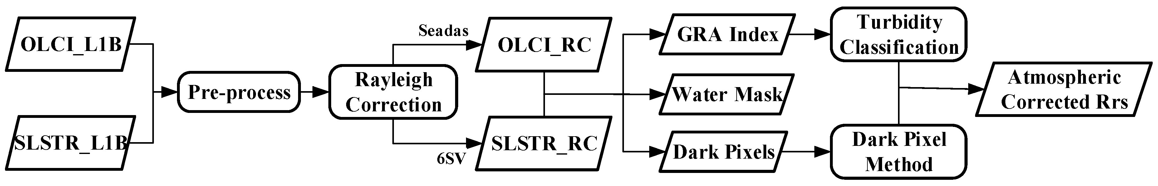
3.2. The Processing Procedure of the ACbTC

Processing procedure of the ACbTC algorithm in this study is mainly divided into three steps (Figure 3): First, the image was pre-processed according to Section 2.2.1; second, the Rayleigh correction was conducted by Seadas LUTs and 6SV for OLCI and SLSTR, respectively; and, lastly, the aerosol reflectance was calculated based on turbidity detection by the GRA index using the dark pixel method [11] according to Section 3.1.

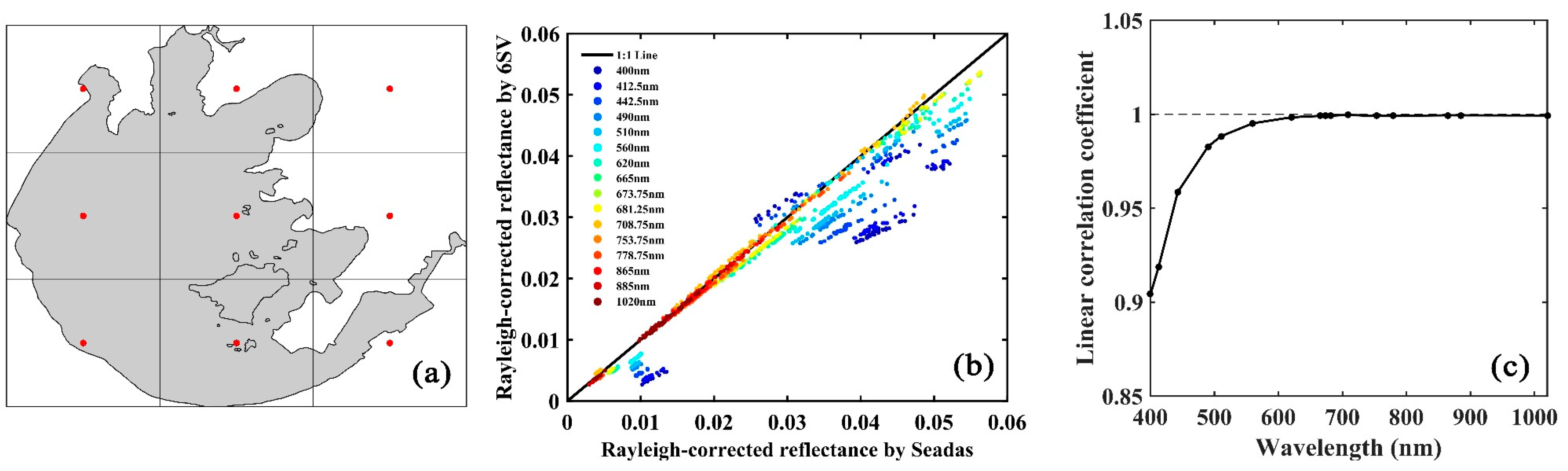
3.2.1. Rayleigh Correction for the OLCI and SLSTR

The Rayleigh correction for OLCI is performed by Seadas LUTs to facilitate the atmospheric correction in Seadas (i.e., MUMM). However, the latest version of the Seadas does not support the Rayleigh correction for SLSTR. Thus, the bands of SL05-1613 nm and SL06-2250 nm were Rayleigh corrected using the 6SV model. To reduce the number of calculations, several points were selected to calculate the Rayleigh scattering, which represents the whole area:

(1)

The smallest rectangle containing the lake area was divided into several squares of the same size (the number of squares depends on the computing ability and the number in this study was selected as nine), and the center pixel of each square was set as the representative point (shown in the Figure 4a).

(2)

The corresponding auxiliary information of each point were extracted from the SLSTR dataset.

(3)

The 6SV model was compiled for each point to simulate the scattering process of the Rayleigh molecules in advance. Then, the Rayleigh reflectance spectrum was constructed and it was assigned to represent this square area.

(4)

In each square, the reflectance of the top of the atmosphere was subtracted from the Rayleigh reflectance to complete the Rayleigh scattering correction.

To analyze the difference between the two Rayleigh correction methods, the Rayleigh correction was performed by using both methods for OLCI bands. The corresponding Rayleigh correction results of 72 in situ points were selected for linear analysis (Figure 4b,c). The results show that the linear correlation coefficient becomes closer to 1 with the increasing wavelength and the results from Seadas and 6SV are similar at longer wavelengths. Due to the weak Rayleigh scatter effect at long wavelengths [45], the 6SV can be used to supplement Seadas at SL05-1613 nm and SL06-2250 nm.

3.2.2. Aerosol Reflectance Calculation by Turbidity Detection

To calculate the aerosol reflectance, the dark pixel should be selected, and the parameter C should be estimated depending on the zero water contribution.

(1) Dark pixel selection

Some studies determine the dark pixels directly by defining thresholds [19]. However, this method is limited by spatial objects and is not suitable for groups of lakes. In this study, histogram statistics of water pixels are used to ensure that the darkest (cleanest) pixels can be found in each study area. The specific three steps are as follows:

(a)

Exclude the boundary between water and land using the Canny filter [61] to avoid the mixed pixel contamination;

(b)

Undeterred by the complex and diverse geographical environments of the images, more stringent taxonomies are established based on NDWI [62] to separate the water pixel from the ice, snow and clouds. The thresholds are determined by the strict visual interpretation in this study [29]:

$$\mathrm{Water}\mathrm{Pixel}\mathrm{is}\{\begin{array}{l}[{\mathrm{R}}_{\mathrm{rs}}(510)-{\mathrm{R}}_{\mathrm{rs}}(1613)]/[{\mathrm{R}}_{\mathrm{rs}}(510)+{\mathrm{R}}_{\mathrm{rs}}(1613)]<0\\ {\mathrm{R}}_{\mathrm{rs}}(1613)<{\mathrm{R}}_{\mathrm{rs}}(1020)<0.02\\ {\mathrm{R}}_{\mathrm{rs}}(1613)<0.01\end{array}$$

(7)

(c)

The intersection of the two 10th percentiles of OL17-865 nm and SL05-1613 nm [8,18,19] is determined as the threshold for dark pixels selection.

(2) Turbidity detection by the GRA index

The band pairs need to be determined when Equation (6) is used to calculate the aerosol reflectance. For this purpose, the GRA index was proposed to detect the water turbidity and, then, the different band pairs were fixed for the clean or turbid waters.

A large amount of Rayleigh corrected images show that there is a clear morphological spectrum difference between clean and turbid water in the NIR-SWIR range. Thus, the GRA index was promoted to identify the turbid water by calculating the difference between the gradient of OL18-885 nm to OL21-1020 nm and that of OL18-885 nm to SL05-1613 nm. The GRA can be calculated by Equation (8) as follows:

$$\begin{array}{l}\mathrm{GRA}=({\mathrm{GRA}}_1+{\mathrm{GRA}}_2)\times {10}^4\\ {\mathrm{GRA}}_1=[{\mathrm{R}}_{\mathrm{rs}}(885)-{\mathrm{R}}_{\mathrm{rs}}(1020)]/(885-1020)\\ {\mathrm{GRA}}_2=[{\mathrm{R}}_{\mathrm{rs}}(885)-{\mathrm{R}}_{\mathrm{rs}}(1613)]/(885-1613)\end{array}$$

(8)

where R_rs(885), R_rs(1020), and R_rs(1613) are the Rayleigh corrected remote sensing reflectance of the OL18-885 nm and OL21-1020 nm and SL05-1613 nm, respectively. The numbers 885, 1020, and 1613 are the center wavelengths (nm) of the above corresponding bands.

To determine the threshold of GRA for turbidity classification, statistical analysis of the histograms were performed by visually interpreting 5000 pixels of both turbid and clean lakes. It is reasonable to set −0.07 as the threshold of the GRA to efficiently distinguish clean or turbid water in this study (Figure 5). The overlap of columns for Turbid and Clean with the limited quantity, which accounts for ~0.98%. Additionally, the histogram statistics of all pixels of the study lakes also have a clear distinction at −0.07. Finally, we temporarily define −0.07 as the threshold of the GRA. Thus, a pixel with a GRA < −0.07 is considered as turbid water. Otherwise, it belongs to the clean water category.

(3) Aerosol correction by different band pairs

For turbid waters, the assumption of water reflectance approaching zero is invalid when the wavelength is longer than 1000 nm, so the calculation of aerosol reflectance is required for SL05-1613 nm and SL06-2250 nm, while, for clean waters, the combination is OL17-865 nm and SL05-1613 nm since the assumption is valid in these wavelengths (see the related procedure in Equations (4)–(6)).

3.3. Accuracy Assessment

The statistical analysis considered the comparison between the in-situ measured R_rs vs. OLCI-derived R_rs. Six popular indices, namely, the MAPE, MRPE, RMSE, slope, intercept, and Pearson correlation coefficient, were used for assessing the accuracy of atmospheric correction. The MAPE, MRPE, and RMSE are defined as Equations (9)–(11), respectively:

$$\mathrm{MAPE}=\frac{100}{N}{\displaystyle \sum _i^N\left|\frac{y_i-x_i}{x_i}\right|}$$

(9)

$$\mathrm{MRPE}=\frac{100}{N}{\displaystyle \sum _i^N\left(\frac{y_i-x_i}{x_i}\right)}$$

(10)

$$\mathrm{RMSE}=\sqrt{\frac{{\displaystyle {\sum }_i^N{(y_i-x_i)}^2}}{N}}$$

(11)

where x_i and y_i are the in situ measured and OLCI-derived reflectance for the ith sample site and N is the number of samples.

4. Results

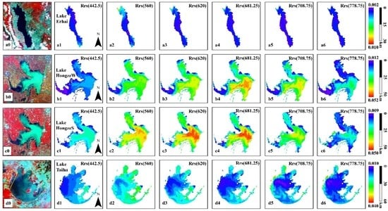
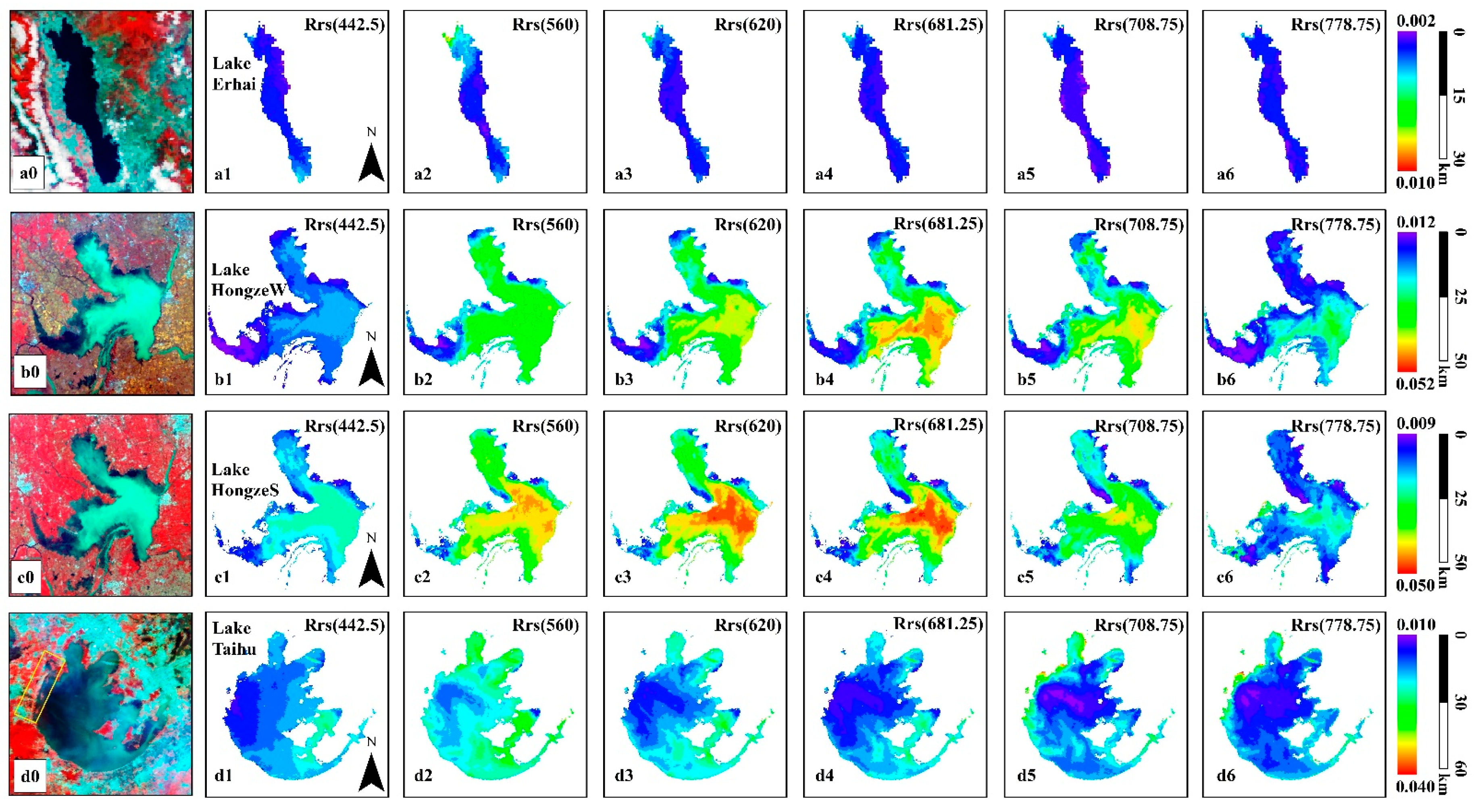
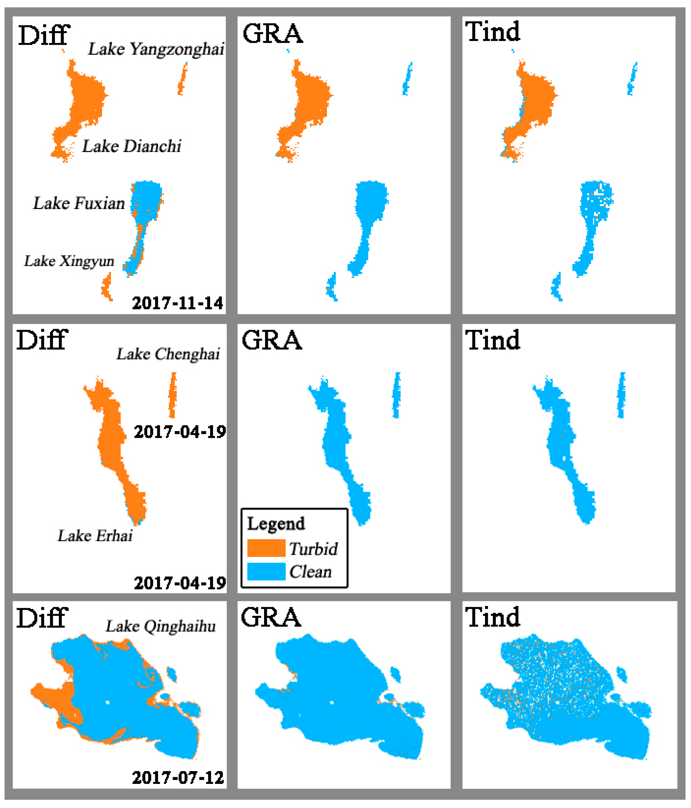
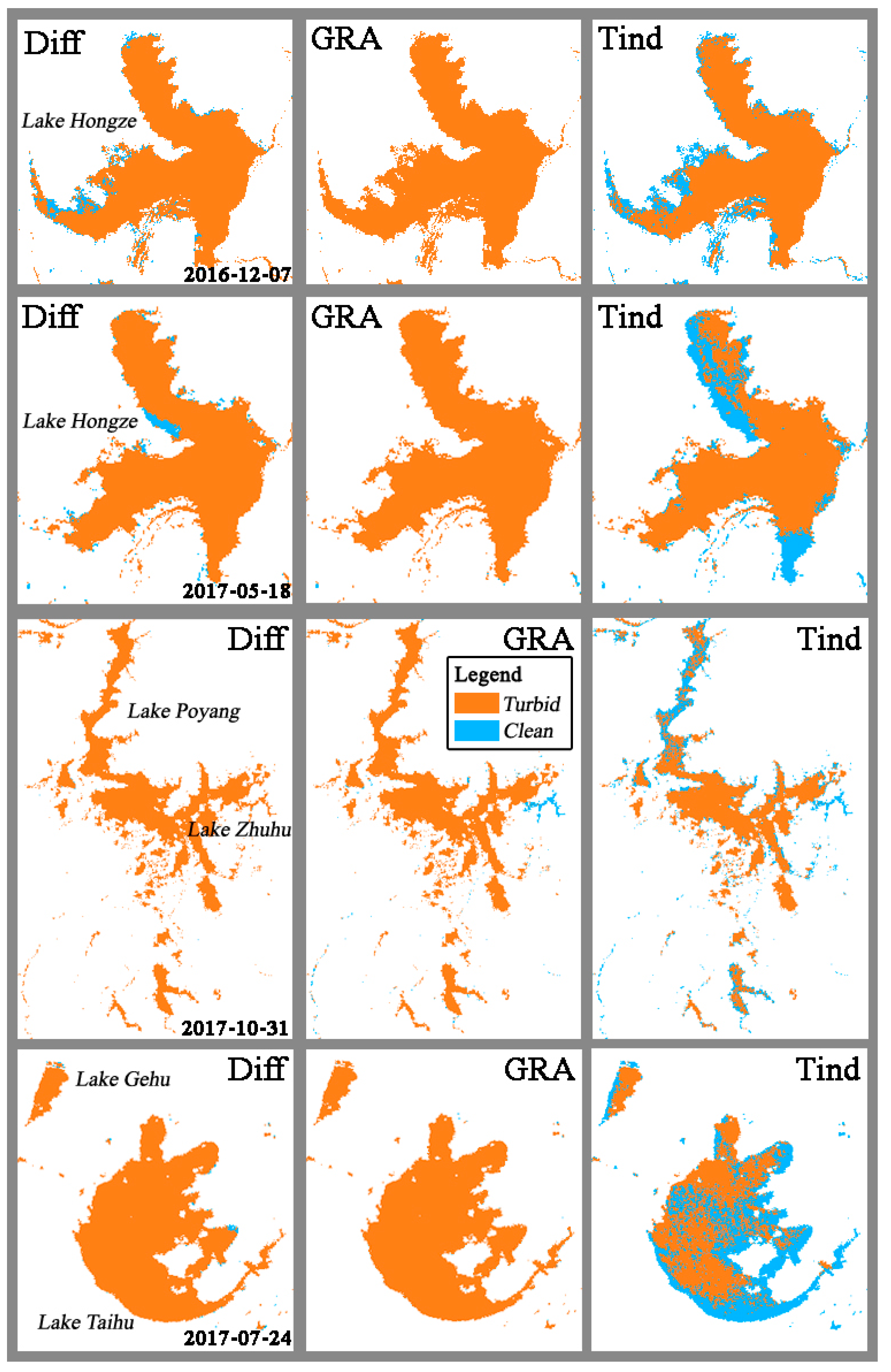
4.1. Visual Inspection of Atmospherically Corrected Images

The original images of false color and the R_rs of the selected bands corrected by ACbTC of Lake Erhai, Lake Hongze and Lake Taihu are shown in Figure 6. The presented six bands are common water color bands, of which 442.5 nm is the characteristic band of Colored Dissolved Organic Matter (CDOM) where the absorption of CDOM and Non-Algal Particulate (NAP) predominates [63]; 560 nm and 708.75 nm are, respectively, the first and second reflection peak positions of Chla; 620 nm is the position of the absorption peak of phycocyanin; and 778.75 nm is commonly used for the estimation of TSM in turbid inland lakes [27]. These six bands can describe the R_rs of the entire OLCI bands and provide a qualitative analysis for atmospheric correction. The area of cyanobacteria blooms in Lake Taihu (Figure 6d0), highlighted in the yellow rectangle, was masked to improve the interpretability of the R_rs images from the western part to ZSB.

From the studies [26,29,64] and our in situ measurement data (Table 1), Lake Erhai is the cleanest among the three lakes but Lake Hongze and Lake Taihu are all dominated by suspended matter. Additionally, Lake Taihu is dominated both by suspended matter and algae which is more eutrophic in summer than Lake Hongze [63]. The maximum R_rs values of Lake Hongze and Lake Taihu are, respectively, 681.25 nm and 560 nm, which correspond to the fact that they are dominated by optically-active substances, while their minimum values are 778.75 nm and 681 nm due to the strong absorption of pure water and pigment, respectively. These results mean that the atmospherically-corrected R_rs at different bands corresponds to the water quality status according to previous studies [26,29,64].

As shown in Figure 6a1–a6, the ACbTC-corrected R_rs values of the six bands in Lake Erhai range from 0.002 to 0.01 sr⁻¹. The image of R_rs(442.5) presents high values (~0.004 sr⁻¹) in the southern area. However, the images of the other bands present high values in the northern region, of which the highest is R_rs(560) with the broadest coverage. The high R_rs occurs because the northern part of Lake Erhai is the area where the algal bloom is most likely to occur [26,64] and R_rs(560) is sensitive to Chla concentration. With the increasing wavelengths, the R_rs of Lake Erhai tends to be spatially homogenous (~0.002 sr⁻¹) over most of the area in 708.75 and 778.75 nm. The magnitude and spatial distribution of R_rs in Lake Erhai after ACbTC are the same as those of the previous studies [64].

The images of Lake Hongze obtained in 7 December 2016 and 18 May 2018 are shown in Figure 6b0–b6,c0–c6, respectively. Lake Hongze (Figure 6b0,c0) is the most turbid of the three lakes, but it is visually cleaner in west LHB, which is mainly covered by wetlands [42]. After the atmospheric correction, the images of the two seasons both show strong spatial heterogeneity at the six bands. The west LHB has the lowest full-band value, close to 0.012 sr⁻¹, while the center is the most turbid at 681.25 nm, approaching 0.05 sr⁻¹. Among them, the spatial distribution heterogeneity of R_rs(778.75) is the strongest, mainly due to the dominant absorption of pure water in these wavelengths, the weak absorption of particulates, and the strong particulate scatter effect, which can efficiently represent the distribution of the TSM concentration [42].

Among the six bands of the ACbTC-corrected results of Lake Taihu, the R_rs(560) is locally the highest, approximately 0.032 sr⁻¹ in MLB, GHB, and XKB, showing that the dominant optically-active substance of these parts of Lake Taihu are algal particles, which is consistent with previous investigations [3,6,21,53]. In the images of R_rs(620) and R_rs(681.25), the value of XKB is high, which is consistent with the water quality characteristics dominated by suspended matter [65]. The lower R_rs(442.5), ~0.01 sr⁻¹, is observed near the area of the algal bloom, which is mainly affected by the strong absorption of pigment particles. Additionally, the high values appearing in 708.75 and 778.75 nm show the characteristic spectrum of algal blooms. In general, Lake Taihu (Figure 6d0) is cleaner in the west to the central area, while more turbid in the eastern part, including XKB and ETH. Additionally, the lower R_rs of the six bands in the center of Lake Taihu is consistent with the observation of Wang et al. [3] where the dark pixels were selected in this study.

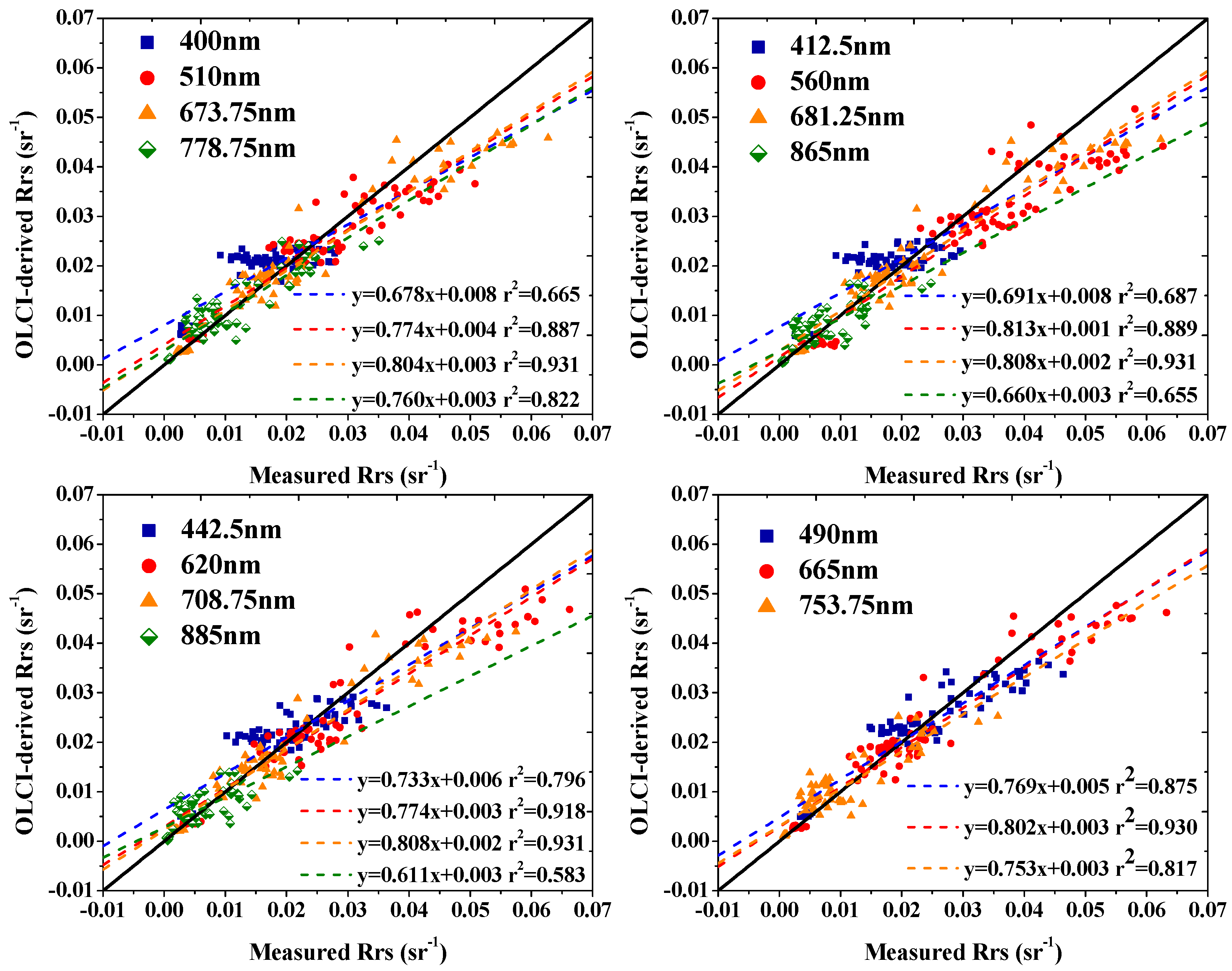
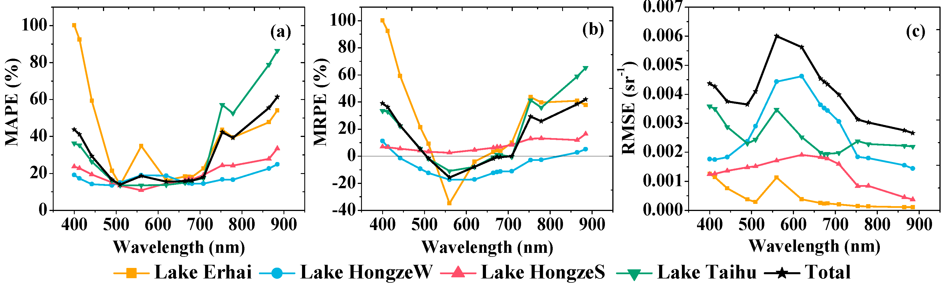
4.2. Comparison with In Situ Measurements

To quantitatively assess the accuracy of the proposed algorithm, the in situ measured and atmospherically-corrected R_rs values were compared. Due to the relatively stable condition of inland lakes [66], the time window between in situ measurements and the satellite overpass was relaxed to ±6 h to obtain a sufficient number of coincident matchup pairs [50,67]. To avoid sub-pixel light contamination, the OLCI-derived remote sensing reflectance (R_rs) values were extracted using a 3 × 3 average pixel-box. The coefficient of variation (CV) of each pixel-box was less than 3% to ensure their homogeneity [51]. Additionally, the sampling sites within two pixels from the shore were excluded to avoid land-adjacent effects based on prior knowledge [29]. To match with the OLCI data, the in situ spectra were convolved to represent the spectra of OLCI using a method referred from the literature [27].

Figure 7 presents the scatter plots of the in situ measured and OLCI-derived R_rs values. Overall, the scattered dots are concentrated near the 1:1 line. Notably, the scattering dots of 400 and 412.5 nm show a flat distribution that means the ACbTC algorithm fails to distinguish the different water conditions. For these two bands, the OLCI-derived and ASD-measured CV are, respectively, approximately 4.5 and 26% (Lake Taihu), 8.0 and 22% (Lake Hongze), and 28 and 40% (Lake Erhai). We attribute this to the following two aspects: (1) the spatial heterogeneity of the Rayleigh and aerosol scattering mainly occurs in the shortwave bands, while the assumption of our algorithm is incapable of that [45]; and (2) the aerosol correction parameter, C, in the dark pixel method is calculated by fitting the reference bands through the exponential function, so the error is relatively large when extrapolated to the short wavelengths, as shown in Equation (6), leading to inaccurate aerosol estimation [11]. However, scattering dots begin to show a more uniform distribution from 490 nm onward, indicating that the OLCI-derived results begin to reflect the difference between sampling measurements. Additionally, the overcorrection occurs between 500 and 700 nm when the measured R_rs is greater than 0.035 sr⁻¹, especially in the more turbid areas (e.g., Lake Hongze). The overcorrection may be due to the non-aerosol signal remaining in the reference bands, resulting in the overestimation of the aerosol reflectance. However, these overcorrections are within an acceptable range, and there are similar correction results in these bands in previous studies based on the dark pixel method [18,55,68].

The relationship of the ACbTC results between the total data and each lake is shown in Figure 8. Note that only MAPE, MRPE, and RMSE values were analyzed in this part due to the apparent optical deviation between the study lakes (Table 1). The full-band average values of MAPE, MRPE, and RMSE are 29.55%, 13.98%, and 0.0039 sr⁻¹, respectively. The total MAPE values decrease from 400 to 510 nm, held steady from 510 to 708.75 nm, increase gradually from 708.75 nm, and reach the maximum at 885 nm. There are four MAPE local maximums at 400, 560, 753.75, and 885 nm which are mainly caused by Lake Erhai and Lake Taihu, as shown in Figure 8a. However, Lake Taihu, Lake HongzeW, and Lake HongzeS maintain the low MAPE values from 400 to 708.75 nm and Lake Taihu performs worse than Lake Hongze. The MRPE values of both Lake Erhai and Lake Taihu show very high, from 400 to 442.5 nm, and the local minimum at 560 nm, which indicates the undercorrection and overcorrection by ACbTC, respectively. The MRPE values of Lake Hongze are better than the other lakes. The total RMSE value at 400–442.5 nm is contributed from Lake Erhai and Lake Taihu. The two causes of this high error in the NIR of Lake Erhai and Lake Taihu are as follows: (1) the NIR water signal in Lake Erhai is weak and susceptible to land-adjacent effects, causing the algorithm to ineffectively eliminate the signal of aerosols [31]; and (2) dominated by suspended matter and algae, Lake Taihu presents considerable spatial heterogeneity in the optical properties in the NIR. Furthermore, Lake Taihu may not satisfy the assumption of the dark pixel method of spatial average for its relatively large area [69]. These two factors may contribute to the poor atmospheric correction performance of Lake Taihu in the NIR.

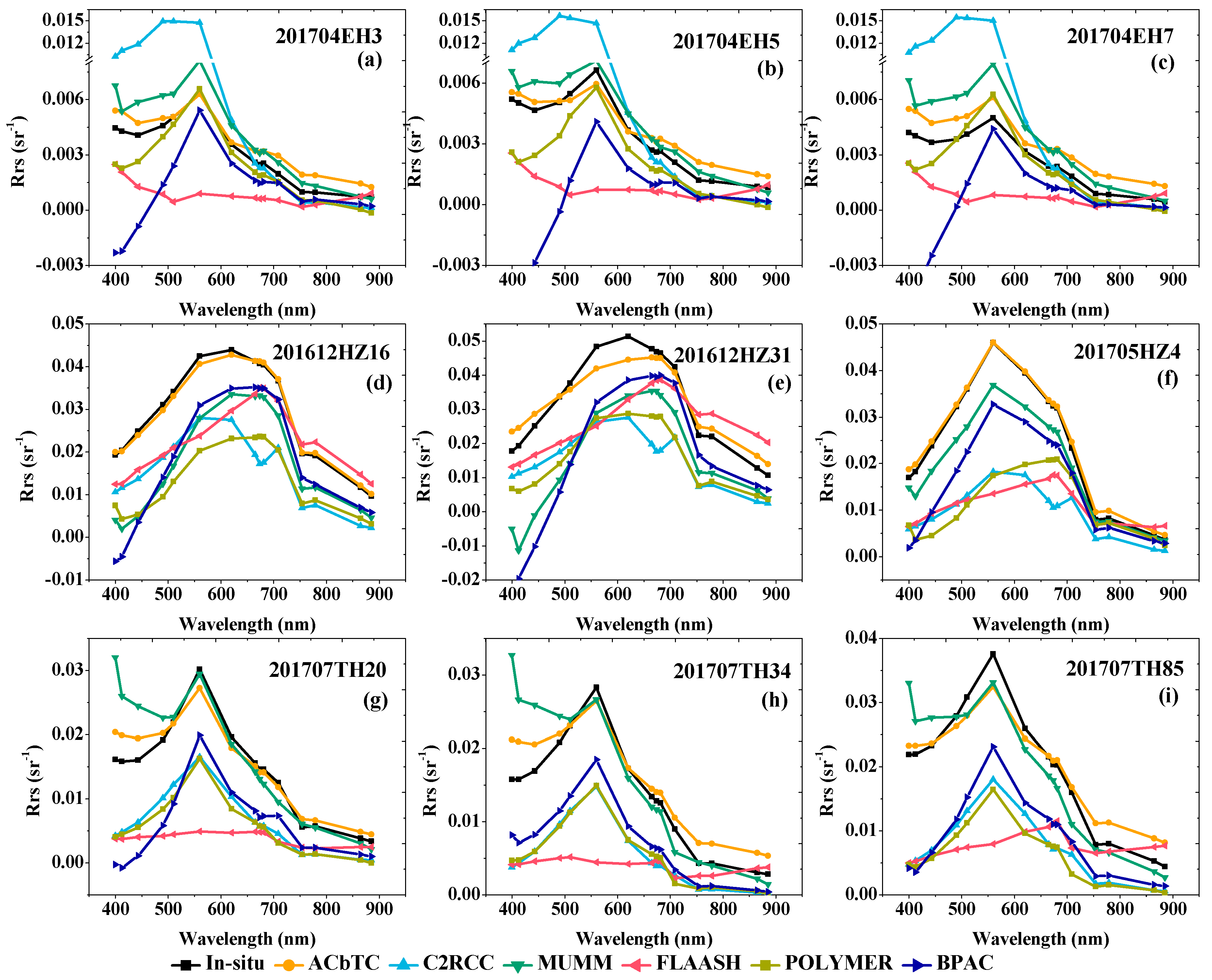
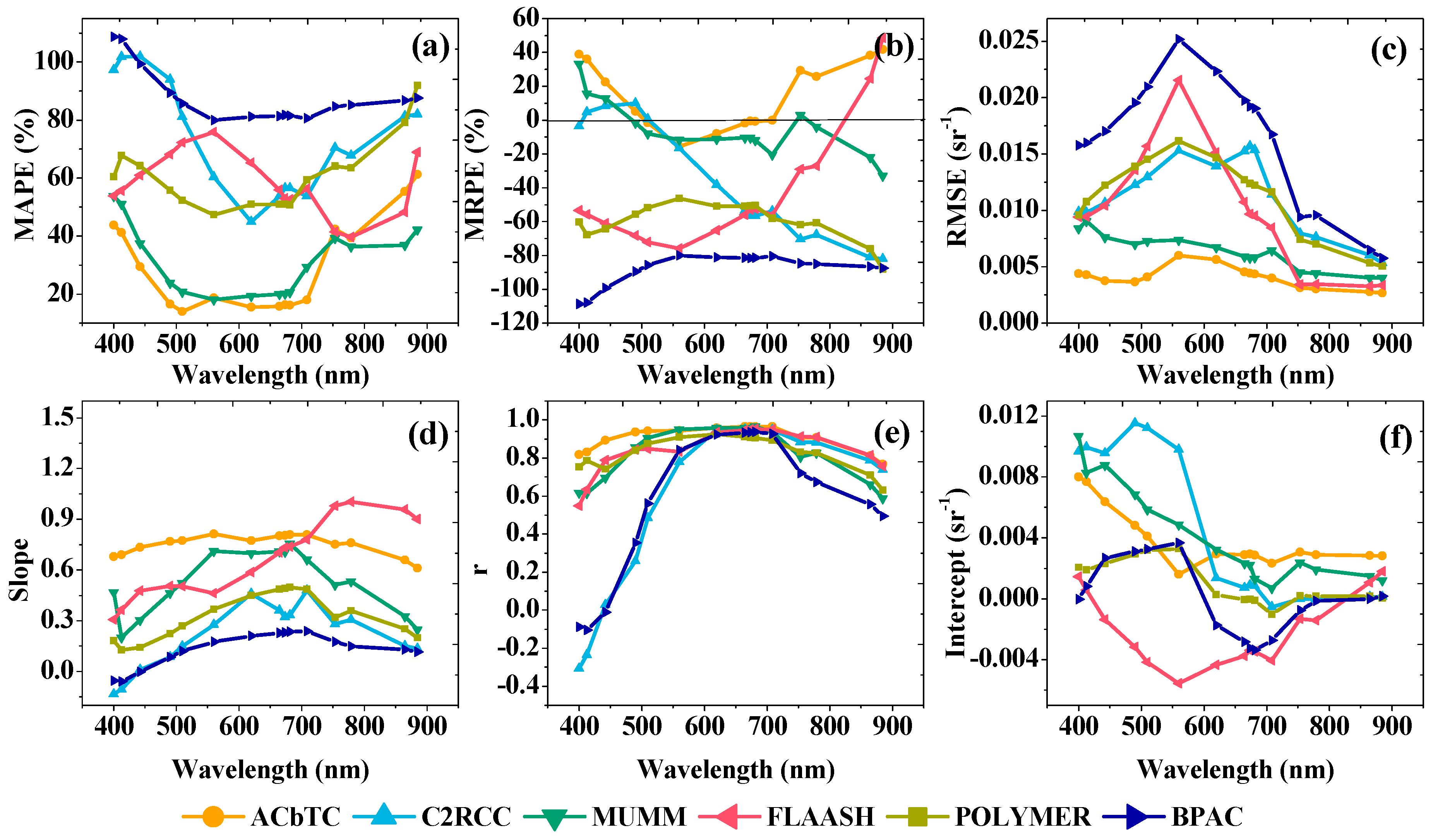
4.3. Comparison with Other Atmospheric Algorithms

To assess the performance of the proposed ACbTC algorithm, the atmospheric correction results of the FLAASH, MUMM, C2RCC, POLYMER, and BPAC were compared in this section from the spectral shape and the magnitude of R_rs. Figure 9 shows a stricter comparison for analysis of the spectral shape between the in situ R_rs values (n = 9) and different atmospheric correction results for a match-up time window of less than 1 h [18,70,71]. Figure 10 presents the comparison of ACbTC with other atmospheric algorithms in MAPE, MRPE, RMSE, slope, r, and intercept (n = 72).

As shown in the Figure 9a–c, the R_rs values derived by FLAASH are far lower than those of the in situ R_rs values from 400 to 708.75 nm, indicating that FLAASH overcorrects the R_rs in Lake Erhai. The same situation occurred in Lake Hongze (Figure 9d–f) and Lake Taihu (Figure 9g–i). However, FLAASH works well in NIR bands in the sediment-dominated Lake Hongze validating that its application for TSM/SSD estimation bands (nearing NIR) in turbid inland lakes is suitable [27,72]. This improvement leads to a gradual decrease of MAPE and MRPE of FLAASH after 708.75 nm (Figure 10a,b). Although the R_rs value trend of C2RCC is similar to that of the in situ R_rs, these results present the most severe deviation (the undercorrection in Lake Erhai and the overcorrection in Lake Hongze and Lake Taihu) and the erroneous correction of the characteristic bands, such as 708.75 nm (Figure 9d–f). The MAPE and MRPE results show that the C2RCC is less effective than FLAASH (Figure 10a,b), the overall bias is the highest of all (Figure 10c), and the regression results also present the worst among all of the algorithms (Figure 10d–f). This is caused by the fact that C2RCC is predetermined by the neural network (NN) method, with the training data mostly simulated by the Hydrolight model [73] and collected from European water [57] whose water constituents and bio-optical features were considerably different from those of the lakes evaluated in this study [57]. MUMM performs better than C2RCC and FLAASH algorithms and has a smaller deviation with the in situ R_rs, even in Lake Erhai (Figure 9a–c). However, MUMM has an overcorrection in Lake Hongze as well and fails to reduce the atmospheric effect in the short wavelength bands in Lake Taihu. The deviation (MAPE, MRPE, and RMSE) of MUMM maintains stability from 500 to 700 nm and the correction result still performs better than C2RCC and FLAASH (Figure 10a–c) showing the stability of MUMM [18]. The error mainly comes from the short bands (<500 nm) which also results in the poor regression outcomes (Figure 10d,e). The overcorrection of POLYMER is observed in all lakes (Figure 10b) but it is reduced in Lake Erhai from 510 to 620 nm (Figure 9a–c). In addition, the overcorrection in Lake Hongze and Lake Taihu becomes more serious compared to C2RCC (Figure 9d–i). This overcorrection indicates that POLYMER may be suitable for clean inland lakes rather than extremely turbid inland lakes. The MAPE of POLYMER is similar to C2RCC after 620 nm, but improves at short wavelengths (Figure 10a) showing more stability than C2RCC. The regression results of POLYMER performs better than C2RCC and FLAASH. In contrast to POLYMER, the BPAC shows serious overcorrection in Lake Erhai (Figure 9a–c). However, the results in Lake Hongze and Lake Taihu are, respectively, similar to those of MUMM (Figure 9d–f) and POLYMER (Figure 9g–i) in spectral shape. The MAPE of BPAC is greater than 80% in the whole wavelength (Figure 10a) and the MRPE is less than −80% (Figure 10b), showing the overcorrection of BPAC in the whole wavelength. This indicates that the IOP models of BPAC might be not suitable for inland lakes in this study. The ACbTC algorithm performs the best, as shown in Figure 9a,b,d,f, and the spectra of the four strict synchronization samples match very well with the in situ R_rs values. Although there is a relative bias in Figure 9c,e, the results of ACbTC are still optimal compared to those of the other algorithms. For three synchronization samples of Lake Taihu, ACbTC has an insufficient correction at short wavelengths as well, but it is better than that of MUMM because its better performance of the spectral shape in NIR. Meanwhile, the MAPE, MRPE, and RMSE of ACbTC are similar with MUMM, but the regression results of the former is better than the latter, as shown in Figure 10d–f.

In summary, FLAASH, C2RCC and BPAC obtained the most inferior results, showing significant differences in the magnitude and spectral shape of the corrected R_rs results, especially before the NIR. Among them, FLAASH slightly improved after the NIR, mainly because of its excellent performance for Lake Hongze. POLYMER performed more stably than FLAASH and C2RCC, but there was a ubiquitous overcorrection phenomenon, especially in turbid lakes. Furthermore, both MUMM and ACbTC showed excellent and stable correction effects, but the latter was more accurate for the overall state of the spectrum, showing better statistical results.

5. Discussion

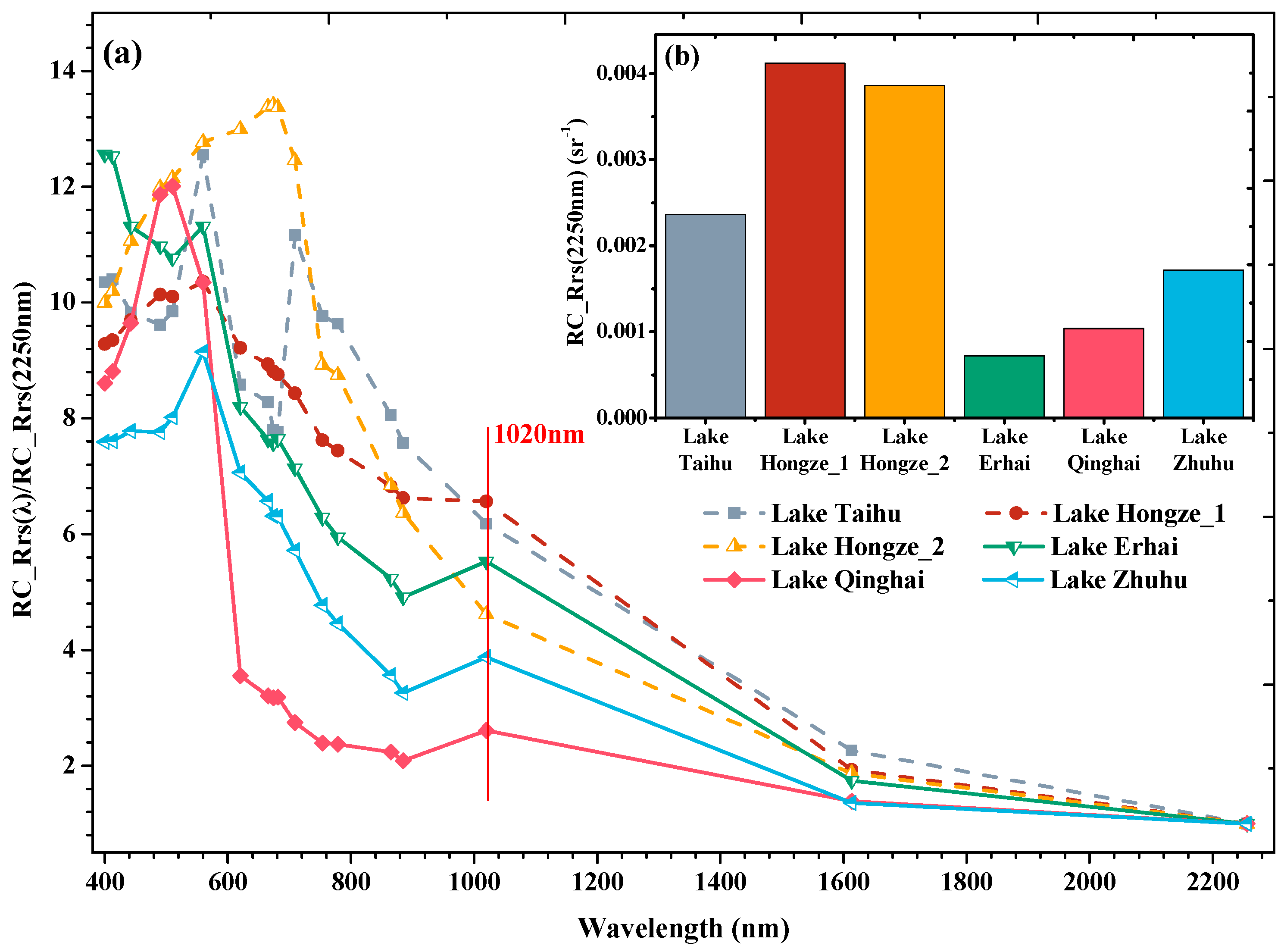
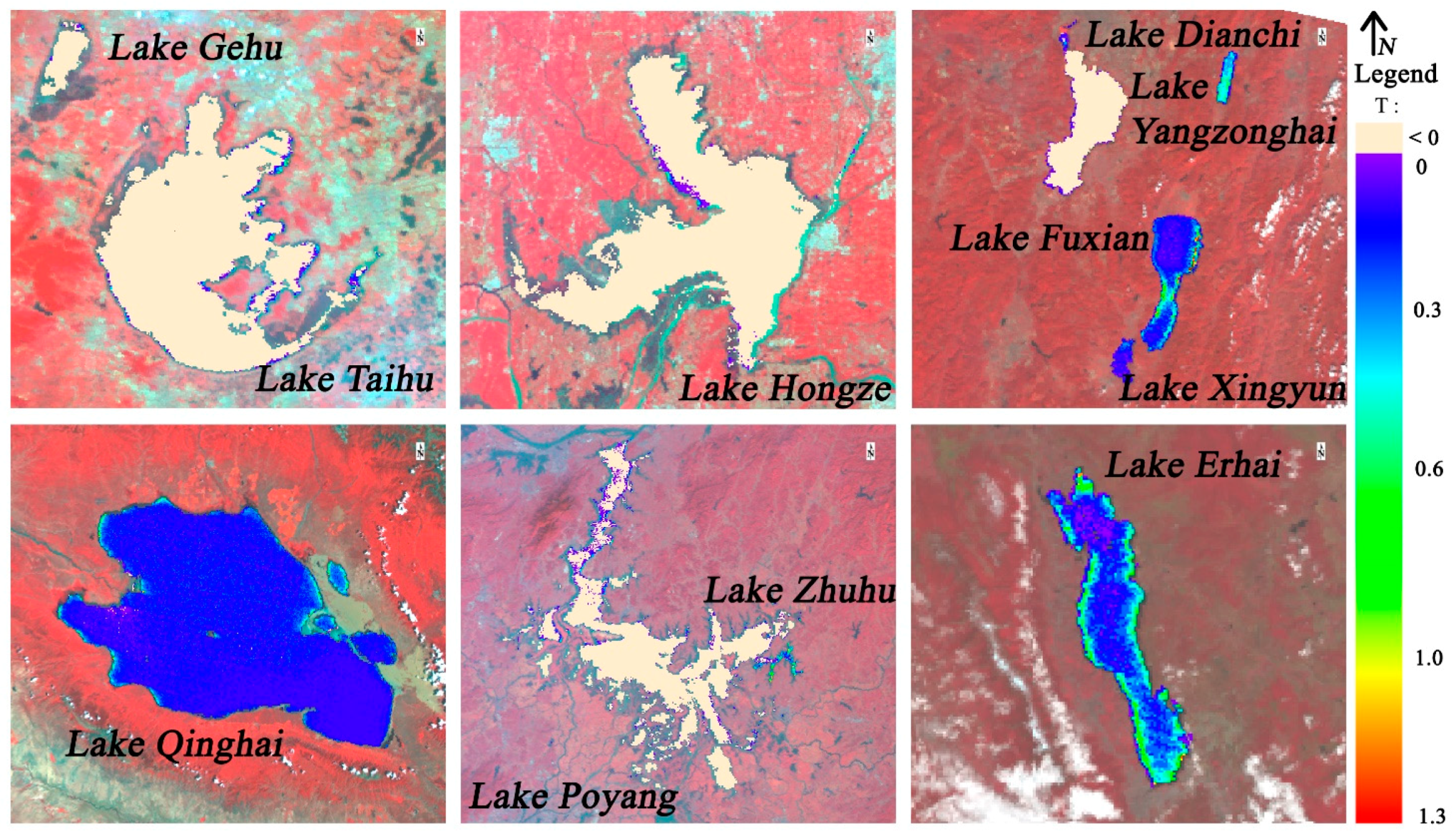
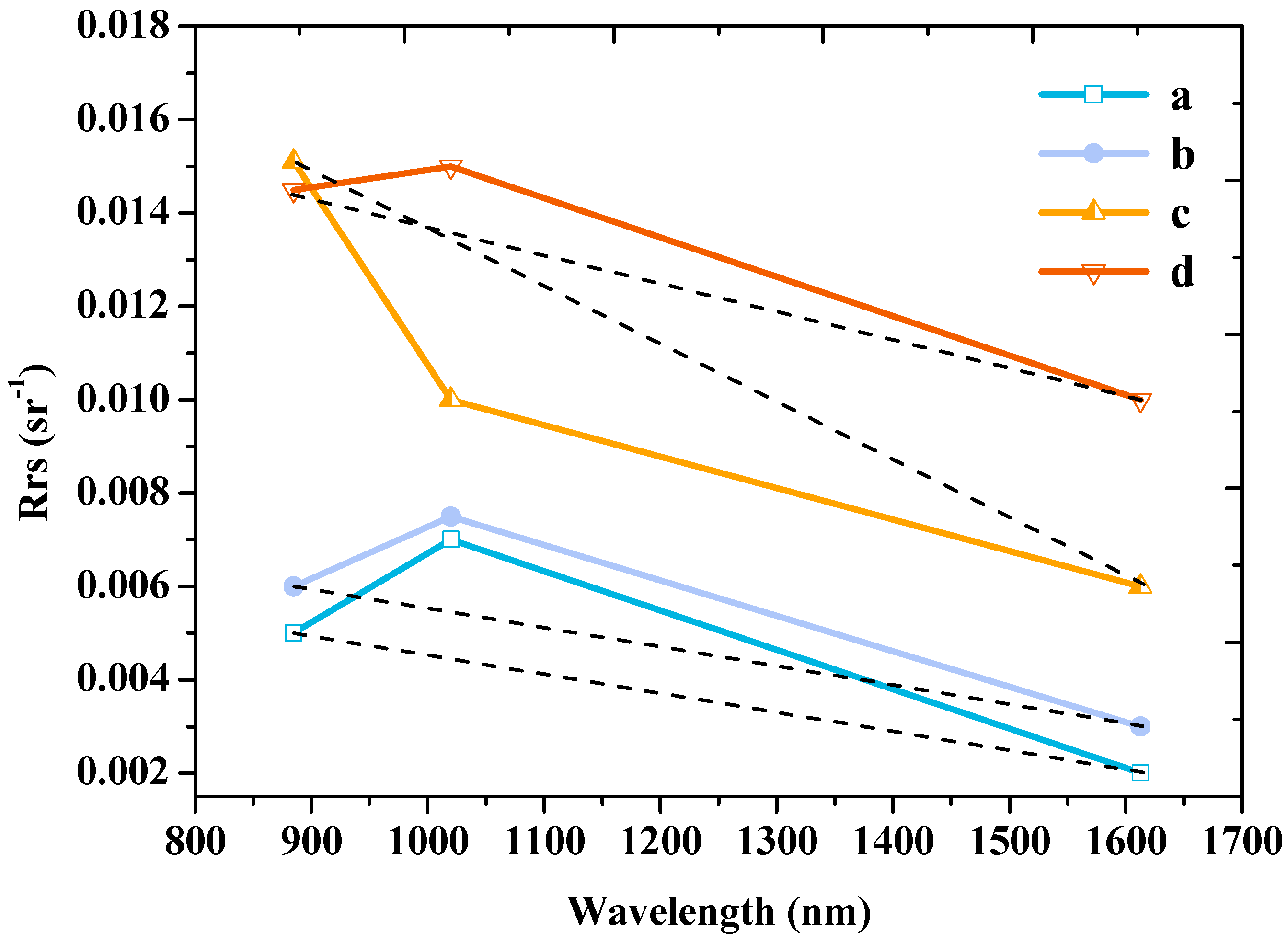
5.1. The Usability of OL21-1020 nm for Distinguishing Turbid Water from Clean Water

The R_rs of OL21-1020 nm was used to detect water turbidity by Equation (8) depending on the weak peak of clean inland water. However, is this band useful for distinguishing between clean and turbid water? By extracting R_rs values from nine Sentinel-3 images (Table 2), a weak peak of Rayleigh corrected R_rs at the 1020 nm band (denoted as the 1020 nm peak) was observed in clean inland water, such as Lake Erhai, Lake Qinghai, and Lake Zhuhu, as shown in Figure 11. Thus, this peak might be an indicator for the identification of these two types of water. To check this hypothesis, a simple normalization index, T, was constructed and applied to the study area for identification. The formula of the T index is:

$$\mathrm{T}=[{\mathrm{R}}_{\mathrm{rsRC}}(1020)-{\mathrm{R}}_{\mathrm{rsRC}}(885)]/[{\mathrm{R}}_{\mathrm{rsRC}}(1020)+{\mathrm{R}}_{\mathrm{rsRC}}(885)]$$

(12)

where R_rsRC(885) and R_rsRC(1020) denote the Rayleigh corrected R_rs in OL18-885 nm and OL21-1020 nm, respectively. When T ≥ 0, the study area belongs to the clean inland waters; otherwise, it is turbid water.

The T values of the surveyed lakes are shown in Figure 11 and are sliced where T ≥ 0. In the turbid lakes, the T values are less than zero in the central region of lakes except in the nearshore region, while, in the clean water, the T values are greater than zero in the central region with a decreasing trend from nearshore region to the lake center. This difference indicates that R_rs(1020) is useful in distinguishing the clean water from the central region of turbid water. However, the nearshore region of the turbid water may be confused with the clean water since the T value is greater than zero there as well (as shown the spectrum of Lake Hongze_1 in Figure 11).

Why is the 1020 nm peak present in the clean water and the nearshore region of turbid water? Is this peak caused by the water signal or a non-water signal? To answer these questions, the absorption and backscattering coefficient of pure water was first analyzed. The absorption spectrum of pure water presents the first absorption peak at 972 nm and an apparent absorption valley at 1071 nm [74,75], while the backscattering coefficient is consistent after 800 nm that means the peak may be caused by other components in the water or by the effect of the shore reflectance spectrum. Since there are very low concentrations of Chla and TSM in the clean water (Table 1), the peak is mainly caused by the impact of land stray light [76,77,78,79], which is also called the land adjacent effect [80,81,82]. Therefore, images of the T index can also characterize the impact of land stray light on the water signal. The land stray light has a different effect on the reflectance of 1020 nm in all the images surveyed in this study, mainly due to the geo-location of view, the atmospheric condition, the lake area, land cover type, and ground elevation [80]. The sag ponds, such as Lake Fuxian, Lake Erhai, and Lake Dianchi, are always surrounded by high altitude mountains whose dense vegetation cover and snow cover can contaminate the 1020 nm signal of the water surface [76,77,83]. As shown in Figure 12, the T values of Lake Erhai, relatively small in area, shows a clear spatial distribution which gradually decreases from the nearshore to the central region. This result indicates that the contamination of land stray light at 1020 nm decreases with longer distances from the shore. Although there are no high mountains around the Lake Qinghai, the contamination from the vegetation and rocks still exist, as shown in Figure 12.

The plain lakes, such as Lake Taihu, Lake Hongze, and Lake Poyang, were mainly surrounded by vegetation, wetland, and urban land. However, are suffered from the stray light as well, as shown in Figure 12. For turbid water, previous studies have proved that the backscattering of sediments in highly turbid water is not close to zero even in the vicinity of 1071 nm [30,31,84]. Therefore, the higher reflectance at 885 and 1020 nm will weaken the influence of land stray light when the distance is far from the land. This phenomenon is present in Lake Hongze_2, as shown in Figure 11. However, when near the lakeshore, the peak appears to be due to the stronger stray light caused by the land cover (Lake Hongze_1).

The discussion of the T index shows: first, the signal of 1020 nm is contaminated by land stray light no matter in clean or turbid water; second, turbid water with strong backscatter at 1020 nm will inhibit stray light effect, especially when the water pixels are far from the land; and, third, the clear water is vulnerable to form the 1020 nm peak due to the weaker backscattering. Therefore, the 1020 nm peak could be an indicator to discriminate between clean and turbid water excluding pixels near the shore.

5.2. The Effect of the GRA Index to Distinguish the Water Turbidity

As described in Section 5.1, the T index could not discriminate between clean inland water and turbid nearshore water. Thus, the improvement is required to distinguish the water turbidity more accurately. In fact, the R_rs(885) varies significantly in inland lakes [29,63]. The high R_rs(885) values of turbid water are mainly affected by the backscattering of the particles while the relatively low R_rs(885) values of clean water are affected primarily by the absorption of the pure water. Meanwhile, the R_rs value at 1613 nm is relatively low in the different waters. Four typical water spectra are shown in Figure 13 of which the slope of the turbid nearshore water (spectrum d) is flatter than that of the clean water and the central turbid water from 885 to 1613 nm. Therefore, Equation (8) can efficiently distinguish the turbid water with the combination of the 1020 nm peak detection (GRA₁) and the decreasing gradient (GRA₂).

To evaluate this method, the results of the GRA were compared with other methods, such as the Diff and Tind indices. The Diff index was proposed to classify the turbidity of near-shore water by calculating the difference between the logarithmic gradients of R_rsRC(470) and R_rsRC(660) and that of R_rsRC(470) and R_rsRC(1240) [85,86]. It is assumed that Diff is less than 0 for clean water pixels. The calculation bands of Diff were modified slightly according to the OLCI bands in this study, which are 490, 665, and 1020 nm. The Tind index uses the combinations of MODIS measured radiance or reflectance in the short visible, NIR and SWIR bands to detect the water turbidity area [8,23]. The corresponding bands of OLCI + SLSTR for Tind are 753.75, 1020, and 2250 nm. The pixels of Tind > 1.3 are considered as the turbid (see Equations (13) and (14), respectively):

$$\mathrm{Diff}=\frac{\lg {\mathrm{R}}_{\mathrm{rsRC}}(665)-\lg {\mathrm{R}}_{\mathrm{rsRC}}(490)}{\lg (665)-\lg (490)}-\frac{\lg {\mathrm{R}}_{\mathrm{rsRC}}(1020)-\lg {\mathrm{R}}_{\mathrm{rsRC}}(490)}{\lg (1020)-\lg (490)}$$

(13)

$$\mathrm{Tind}=\frac{{\mathrm{R}}_{\mathrm{rsRC}}(753.75)}{{\mathrm{R}}_{\mathrm{rsRC}}(1020)}\times \exp \left\{-\frac{753.75-1020}{2250-1020}\times \frac{{\mathrm{R}}_{\mathrm{rsRC}}(1020)}{{\mathrm{R}}_{\mathrm{rsRC}}(2250)}\right\}$$

(14)

As shown in Figure 14 and Figure 15, the turbid or clean pixels of the study lakes are distinguished using Diff, GRA, and Tind. The results of plateau lakes are shown in Figure 14, of which only Lake Dianchi is considered to be a turbid lake (Table 1) noting that the pixels in the southern part of Lake Dianchi were masked due to the cyanobacteria bloom. Diff mainly misclassified clean lakes as turbid, such as Lake Yangzonghai, Lake Xingyun, and Lake Chenghai, and locally misclassified the central part of Lake Fuxian and Western Lake Qinghai. Tind performed better than Diff. However, the noise of Tind, which comes from the SL05-1613 nm or SL06-2250 nm in clean water, or the stray light, mainly from the land surface, may affect the judgment in some parts of a lake, such as the western part of Lake Dianchi, Lake Fuxian, and Lake Qinghai. Finally, the GRA proposed in this study can not only effectively classify the whole lake, but can also resist the stray light effect under certain conditions.

In Figure 15, lakes in the middle and lower reaches of the Yangtze River are all sediment-dominated except for Lake Zhuhu (Table 1). The three indices have less misjudgment in general, but more misjudgment at the local level. Among the classification results of Lake Hongze, Tind is the worst and Diff is second, but the GRA is the best. Although central part of Lake Poyang was distinguished as turbid water by Diff and GRA, pixels of the main channel, in the northern region of Lake Poyang, was mistakenly identified as clean by Tind. For Lake Taihu and Lake Gehu, better discrimination can be found in Diff and GRA, in general, although some misjudgment appeared in the eastern region of Lake Taihu. However, there were more misjudged pixels by Tind in Lake Taihu, especially in the nearshore regions.

In general, it is accurate to discriminate water turbidity using Tind, which was also confirmed in the previous research on its application in coastal waters [8]. However, Tind occasionally misjudged the lake turbidity on the local scale, especially for the nearshore pixels. It can be explained that Tind may not be directly applicable to inland lakes though it performed well in the coastal regions [3,53]. Diff performed well in turbid lakes, but it was vulnerable to misjudge the whole lake in clean water. Moreover, the Diff index has poor resistance to hillside reflections and submerged plants in the inland lakes. However, based on the spectral morphology (Figure 13), the GRA performed better than Diff and Tind because it is supported by the characteristics of the 1020 nm peak of clean water. These findings indicate that the method of turbidity classification based on the spectral morphology is simple, but effective.

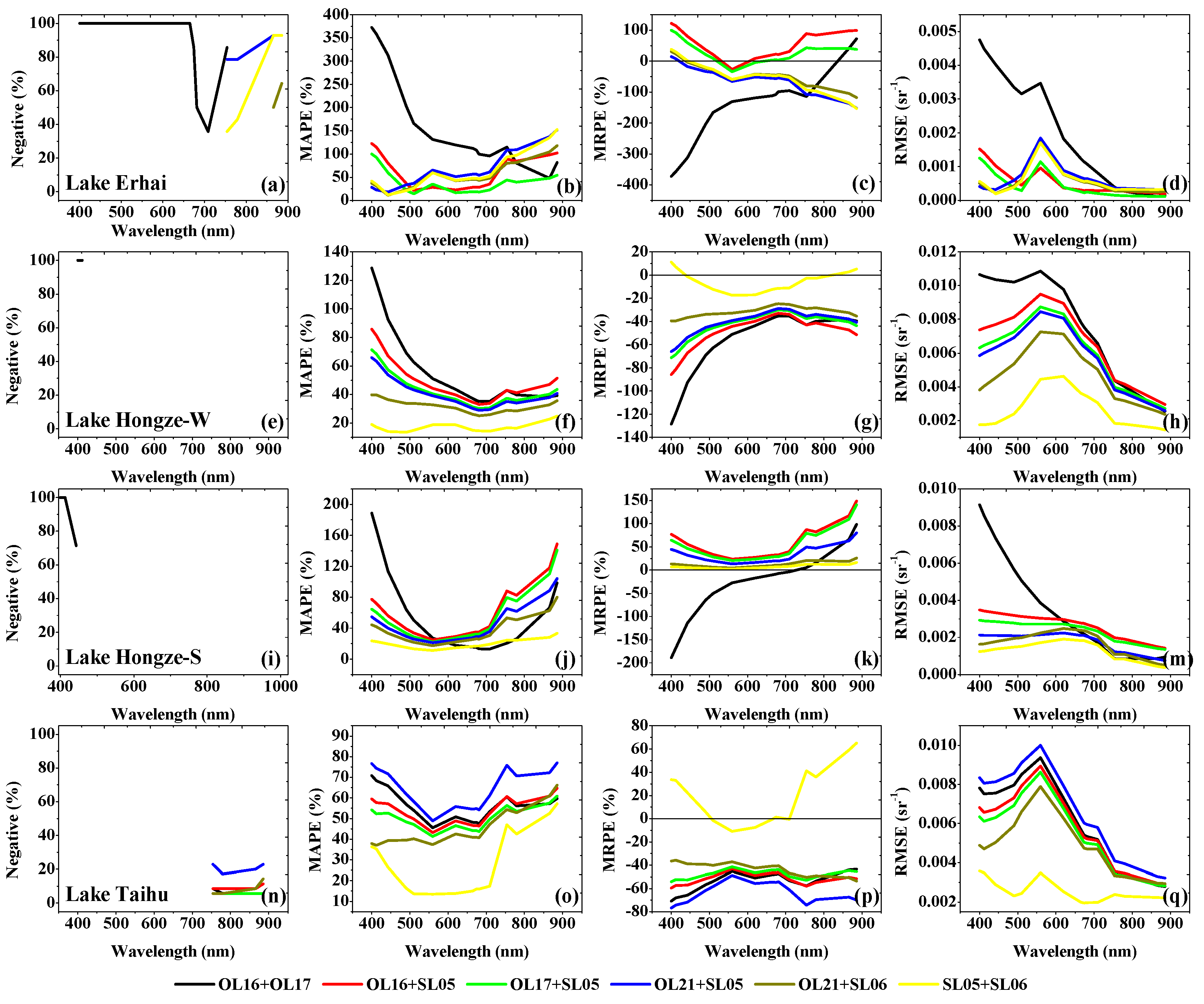
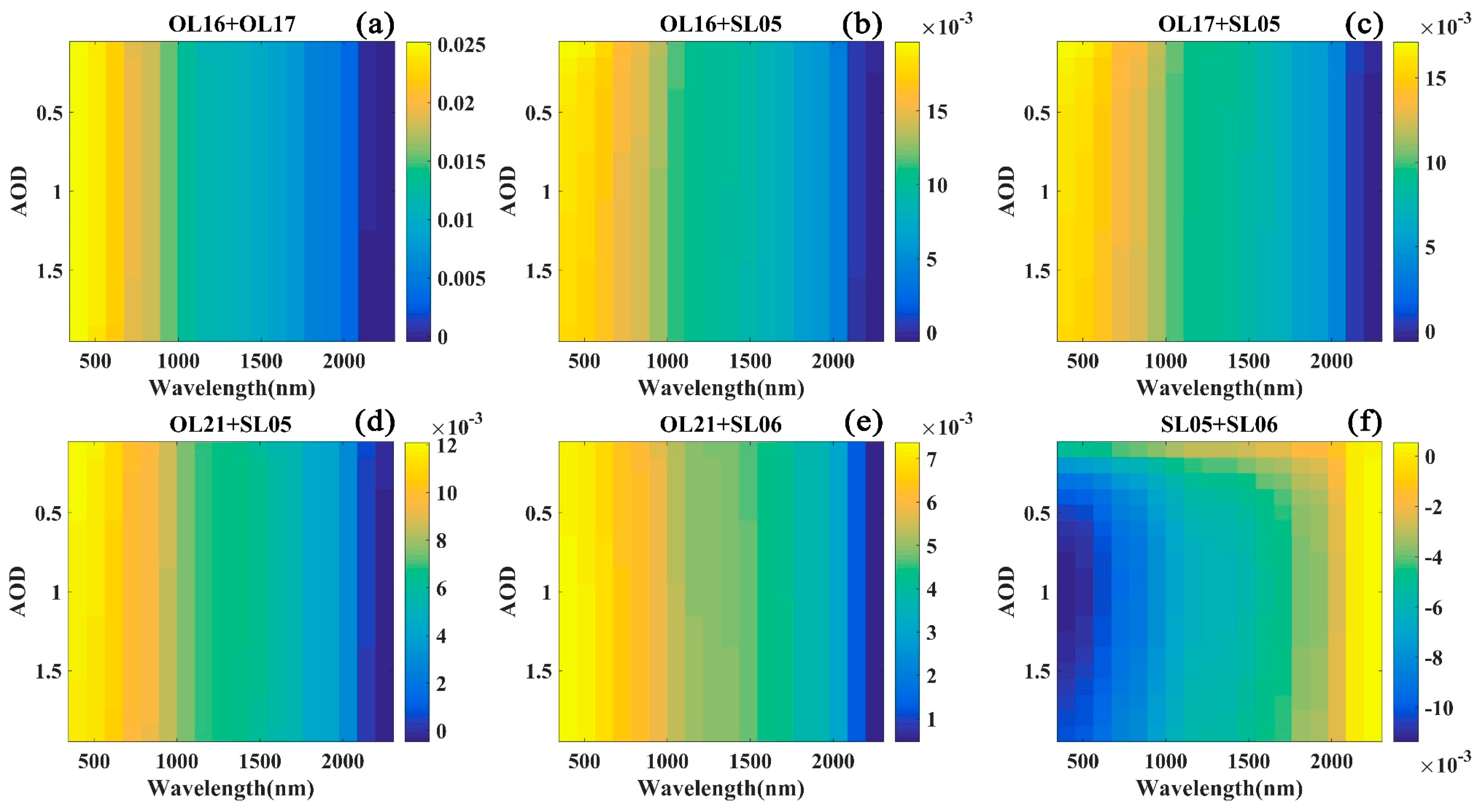
5.3. The Necessity of Using Different Bands for Atmospheric Correction in Turbid and Clean Inland Lakes

To analyze the necessity of band selections for the ACbTC algorithm, six bands were selected, which are the commonly used atmospheric correction bands, from the OLCI and SLSTR: OL16-778.75 nm, OL17-865 nm, OL21-1020 nm, SL05-1613 nm, and SL06-2250 nm [5,6,7,18,53]. Based on the discussion of Section 5.1 and Section 5.2, the OL21-1020 nm band was excluded when paired with the NIR band, as the Rayleigh-corrected R_rs(1020) value in clean water is sometimes even higher than the R_rs in the NIR. Finally, six pairs were generated: OL16 + OL17, OL16 + SL05, OL17 + SL05, OL21 + SL05, OL21 + SL06, and SL05 + SL06, and the atmospheric correction was performed based on these six pairs. Correction results were compared with the in situ measurements and analyzed using negative (the percent of negative values), MAPE, MRPE, and RMSE, as shown in Figure 16. Meanwhile, the full-band average values of these indices are shown in

Table 3. The full-band average values of the MAPE, MRPE, and RMSE of the atmospheric correction results using different band combinations including OL16 + OL17, OL16 + SL05, OL17 + SL05, OL21 + SL05, OL21 + SL06, and SL05 + SL06 The bold font indicates the best combinations.

Index	Combinations	Lake Erhai	Lake HongzeW	Lake HongzeS	Lake Taihu
MAPE (%)	OL16 + OL17	160.02	58.11	59.91	56.19
	OL16 + SL05	61.18	49.45	61.04	53.54
	OL17 + SL05	40.05	43.24	54.91	50.17
	OL21 + SL05	65.78	40.84	45.80	64.52
	OL21 + SL06	53.09	31.70	37.33	45.17
	SL05 + SL06	60.41	17.10	19.95	32.96
MRPE (%)	OL16 + OL17	−143.87	−58.11	−31.44	−53.90
	OL16 + SL05	54.69	−49.45	60.26	−51.63
	OL17 + SL05	28.43	−43.24	53.75	−47.85
	OL21 + SL05	−60.99	−40.84	34.22	−63.58
	OL21 + SL06	−44.35	−31.48	13.01	−42.98
	SL05 + SL06	−49.98	−5.57	7.77	18.39
RMSE (sr−1)	OL16 + OL17	0.00202	0.00772	0.00362	0.00602
	OL16 + SL05	0.00056	0.00667	0.00267	0.00569
	OL17 + SL05	0.00045	0.00604	0.00239	0.00542
	OL21 + SL05	0.00060	0.00578	0.00180	0.00658
	OL21 + SL06	0.00052	0.00476	0.00174	0.00486
	SL05 + SL06	0.00054	0.00267	0.00134	0.00251

.

For the OL16 + OL17, there are negative values in both the short and near-infrared bands, especially for Lake Erhai where the match-up points from 400 to 665 nm are all negative, resulting in poor MAPE, MRPE and RMSE values, as shown in Figure 16b–d. These figures indicate that the band combination of NIR bands, 778.75 and 865 nm, will overcorrect even in clean inland water due to the non-negligible water signal. Moreover, the overcorrection caused by OL16 + OL17 is the most serious in this study with the MRPE far less than zero, which results in higher MAPE and RMSE values. However, the correction results are improved when the band of SLSTR is added to the combination, such as OL16 + SL05 and OL17 + SL05. The most considerable improvement of correction is Lake Erhai, but the turbid water, especially Lake Hongze-W and Lake Taihu, are still overcorrected, which means longer bands are required for atmospheric correction in turbid lakes. Although OL21 + SL05 and OL21 + SL06 perform better than OL16 + SL05 and OL17 + SL05, the combinations including OL21-1020 nm result in the critical overcorrection (even the negative results after NIR) in Lake Erhai. The two combinations perform better for turbid water, such as Lake Hongze and Lake Taihu, but are still inferior to the combination of SL05 + SL06, probably due to a more significant amount of stray light from the water at OL21-1020 nm. This result shows again that the impact of the stray light on the accuracy of atmospheric correction for inland lakes should be considered, and weakening its influence is an essential prerequisite for accurate corrections [82].

As shown in Figure 16a,n, Lake Erhai and Lake Taihu present negative results in the NIR while the proportion of Lake Taihu is smaller than that of Lake Erhai, nearing 5%. To analyze this phenomenon, the aerosol reflectance is numerically simulated based on the 6SV model. The atmospheric model was defined by total column water vapor and ozone, the aerosol model was assumed as “Continental”, and the aerosol optical depth (AOD) ranged from 0.1 to 1.9 to simulate different aerosol conditions [87]. According to the information provided in Section 3.1 and Section 5.1, it is considered that there are three main components in ρ_RC, which are the water signal (ρ_w), the aerosol signal (ρ_a), and the stray light signal (ρ_S). The simulated reflectance of water surface was referred to the average of in situ R_rs in the nearshore of Lake Taihu. The proportion of the stray light, ρ_S/(ρ_r + ρ_a), was assumed as a constant 0.1 reference from previous studies [81,88]. When the dark pixel assumption is satisfied, ρ_RC = ρ_a; otherwise, ρ_RC = ρ_w + ρ_a + ρ_S. Therefore, Equation (6) changes to Equations (15) and (16). Finally, their difference calculated by Equation (17) presents the overcorrection (Δρ_a > 0) or undercorrection (Δρ_a < 0) for the aerosol, respectively:

$$C_T=\ln \frac{{\rho }_a({\lambda }_1)}{{\rho }_a({\lambda }_2)}/({\lambda }_2-{\lambda }_1)\&C_M=\ln \frac{{\rho }_w({\lambda }_1)+{\rho }_a({\lambda }_1)+{\rho }_S({\lambda }_1)}{{\rho }_w({\lambda }_2)+{\rho }_a({\lambda }_2)+{\rho }_S({\lambda }_2)}/({\lambda }_2-{\lambda }_1)$$

(15)

$${\rho }_{T,a}(\lambda )={\rho }_a({\lambda }_1)\cdot \exp [C_T({\lambda }_1-\lambda )]\&{\rho }_{M,a}(\lambda )=[{\rho }_w({\lambda }_1)+{\rho }_a({\lambda }_1)]\cdot \exp [C_M({\lambda }_1-\lambda )]$$

(16)

$$\mathsf{\Delta }{\rho }_a={\rho }_{M,a}-{\rho }_{T,a}$$

(17)

where subscripts T and M denote the theoretical and measured values, respectively [23].

The band combinations including OL16-778.75 nm, OL17-865 nm and OL21-1020 nm (shown in Figure 17a–e) present the overcorrection in short bands which corresponds to Figure 16p. As the reference wavelength increases, the Δρ_a generally decreases showing that the overcorrection is relieved. However, SL05 + SL06 shows an undercorrection which is relieved with the increasing wavelength (Figure 17f). The simulation results show once again that OL16 + OL17, OL16 + SL05, OL17 + SL05, OL21 + SL05 and OL21 + SL06 will overestimate the aerosol signal due to the non-negligible water signal and the land stray light, which universally result in the overcorrection. In addition, the points with negative values mainly distributed in the center of Lake Taihu where the water is much cleaner (Figure 6d5) which could explain the overcorrection and the negative corrected values in Figure 16n. The changes of AOD are less sensitive to these band combinations. On the contrary, SL05 + SL06 will cause the undercorrecton which becomes more serious when AOD in 0.5~1.5. However, there are still more interferences in the actual earth observation by satellites. In this study, the analysis here is only a simple numerical simulation of these phenomena. More in-depth research requires more synchronously in-situ measurement of atmospheric and water surface, especially in the SWIR bands.

As shown in Table 3, OL17 + SL05 is a reasonable band combination for clean inland lakes such as Lake Erhai, whereas SL05 + SL06 is recommended for the more turbid inland lakes such as Lake Hongze and Lake Taihu.

5.4. Limitations of ACbTC in Applications

Although the ACbTC algorithm has certain advantages compared with other atmospheric correction algorithms, the algorithm itself has certain limitations. The algorithm must be evaluated for applicability of the atmospheric correction.

First, the performance of ACbTC at 400 and 412.5 nm in the dataset of this study was not ideal, with total MAPE values of 43.73% and 41.16%, respectively (Figure 7). Lake Erhai is the primary source of error (shown in Figure 8a) whose MAPE values at 400, 412.5, and 442.5 nm reached 100.21%, 92.41%, and 59.29%, respectively. This means the ACbTC algorithm failed to obtain relatively accurate atmospheric correction results at short wavelengths in clean inland lakes where R_rs(778.75) is lower than 0.001 sr⁻¹.

Second, the performance of ACbTC in 753.75–885 nm is not good enough for Lake Taihu, dominated by both suspended sediment and algal particulate matter (Figure 8), and is worse than MUMM (Figure 9g–i), but better in 400–490 nm. This indicates that the atmospheric correction for inland lakes, such as Lake Taihu, is more suitable at short wavelengths using ACbTC, and at NIR wavelengths using MUMM.

Third, for the two seasons of data for Lake Hongze in this study, ACbTC performed best. The MRPE value over the whole band remained at ~17.10% and was stable between 510–778.75 nm (Figure 8). Therefore, the use of ACbTC for atmospheric correction is recommended for inland lakes, such as Lake Hongze (lakes that are dominated by suspended sediments).

Fourth, the upcoming products of Sentinel-3 (such as L1C) are required for synergistic use of OLCI and SLSTR. On the one hand, although the collocation tool of SNAP was used in this study to eliminate the image misregistration of the two sensors, the remaining mismatched pixels (ca. two-pixel distance) will impact the turbidity classification, water pixels extraction, and atmospheric correction [33,89,90]. The future work should discuss the sensitivity of the algorithm to the image misregistration. On the other hand, the first version of the OLCI data was reported to show bias in the blue and NIR so that the SVC is necessary [59,60] for Sentinel-3 products.

6. Conclusions

An improved atmospheric correction method based on the turbidity classification (ACbTC) algorithm using the synergy of OLCI and SLSTR was presented in this study for inland lakes in China.

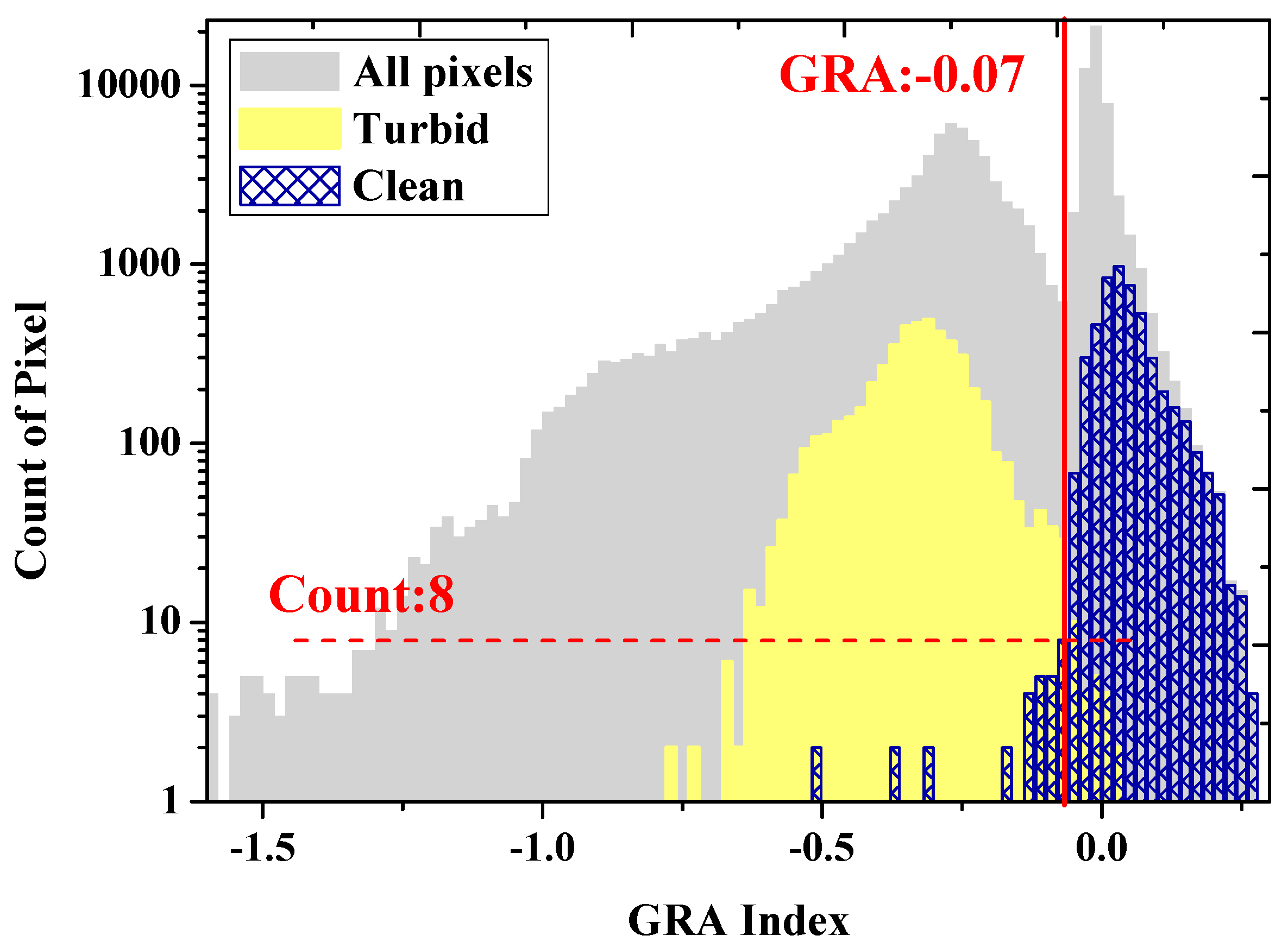
(1)

The GRA index is proposed to distinguish turbid inland water from clean water, which depends on the feature of the 1020 nm peak of R_rs in clean inland lakes and the decreasing slope from 885 to 1613 nm, especially for clean inland lakes that cover relatively small areas. Through the qualitative analysis of 12 inland lakes and the existing observation data, the threshold of the GRA index was determined as −0.07 in this study. The classification results of the GRA index performed better than the Diff and Tind indices for inland lakes by constraining the land adjacency effect at 1020 nm on the similar spectral shapes of turbid lakes.

(2)

The synergistic use of OLCI and SLSTR was verified to provide additional atmospheric correction bands, SL05-1613 nm and SL06-2250 nm, for turbid inland lakes to satisfy the dark pixel assumption. The incorrect use of atmospheric correction bands in turbid inland lakes may cause an overcorrection in the short bands due to the invalid assumption and the stray light effect. Thus, OL17 + SL05 and SL05 + SL06 are recommended for the clean and turbid inland waters, respectively. Additionally, OL21-1020 nm is unsuitable for atmospheric correction of inland lakes because it is a vulnerable band easily affected by land stray light.

(3)

The ACbTC method calculated the aerosol reflectance based on turbidity identification. Compared to the in situ measurements, the ACbTC algorithm achieved full-band average values of MAPE = 29.55%, MRPE = 13.98%, and RMSE = 0.0039 sr⁻¹, which were more accurate than the C2RCC, MUMM, FLAASH, POLYMER, and BPAC. The results indicate that both the synergistic use of OLCI and SLSTR and the water turbidity classification are essential for accurate atmospheric correction in inland lakes when using Sentinel-3 data.

References

- Shi, K.; Zhang, Y.; Zhu, G.; Qin, B.; Pan, D. Deteriorating water clarity in shallow waters: Evidence from long term MODIS and in-situ observations. Int. J. Appl. Earth Obs. Geoinf. 2018, 68, 287–297. [Google Scholar] [CrossRef]
- Shutler, J.; Land, P.; Smyth, T.; Groom, S. Extending the MODIS 1 km ocean colour atmospheric correction to the MODIS 500 m bands and 500 m chlorophyll-a estimation towards coastal and estuarine monitoring. Remote Sens. Environ. 2007, 107, 521–532. [Google Scholar] [CrossRef]
- Wang, M.; Shi, W.; Tang, J. Water property monitoring and assessment for China’s inland Lake Taihu from MODIS-Aqua measurements. Remote Sens. Environ. 2011, 115, 841–854. [Google Scholar] [CrossRef]
- Palmer, S.C.; Kutser, T.; Hunter, P.D. Remote sensing of inland waters: Challenges, progress and future directions. Remote Sens. Environ. 2015, 157, 1–8. [Google Scholar] [CrossRef]
- Wang, M. Atmospheric correction for remotely-sensed ocean-colour products. In Reports and Monographs of the International Ocean-Colour Coordinating Group (IOCCG); IOCCG: Monterey, CA, USA, 2010. [Google Scholar]
- Liu, G.; Li, Y.; Lyu, H.; Wang, S.; Du, C.; Huang, C. An improved land target-based atmospheric correction method for Lake Taihu. IEEE J. Sel. Top. Appl. Earth Obs. Remote Sens. 2016, 9, 793–803. [Google Scholar] [CrossRef]
- Steinmetz, F.; Deschamps, P.-Y.; Ramon, D. Atmospheric correction in presence of sun glint: Application to MERIS. Opt. Express 2011, 19, 9783–9800. [Google Scholar] [CrossRef] [PubMed]
- Wang, M.; Shi, W. The NIR-SWIR combined atmospheric correction approach for MODIS ocean color data processing. Opt. Express 2007, 15, 15722–15733. [Google Scholar] [CrossRef] [PubMed]
- Gao, B.-C.; Davis, C.; Goetz, A. A review of atmospheric correction techniques for hyperspectral remote sensing of land surfaces and ocean color. In Proceedings of the IEEE International Symposium on Geoscience and Remote Sensing, Denver, CO, USA, 31 July–4 August 2006; pp. 1979–1981. [Google Scholar]
- Ruddick, K.G.; Ovidio, F.; Rijkeboer, M. Atmospheric correction of SeaWiFS imagery for turbid coastal and inland waters. Appl. Opt. 2000, 39, 897–912. [Google Scholar] [CrossRef] [PubMed]
- Gordon, H.R.; Wang, M. Retrieval of water-leaving radiance and aerosol optical thickness over the oceans with SeaWiFS: A preliminary algorithm. Appl. Opt. 1994, 33, 443–452. [Google Scholar] [CrossRef] [PubMed]
- Wang, M.; Gordon, H.R. A simple, moderately accurate, atmospheric correction algorithm for SeaWiFS. Remote Sens. Environ. 1994, 50, 231–239. [Google Scholar] [CrossRef]
- Ahn, J.-H.; Park, Y.-J.; Ryu, J.-H.; Lee, B.; Oh, I.S. Development of atmospheric correction algorithm for Geostationary Ocean Color Imager (GOCI). Ocean Sci. J. 2012, 47, 247–259. [Google Scholar] [CrossRef]
- Moore, G.; Aiken, J.; Lavender, S. The atmospheric correction of water colour and the quantitative retrieval of suspended particulate matter in Case II waters: Application to MERIS. Int. J. Remote Sens. 1999, 20, 1713–1733. [Google Scholar] [CrossRef]
- Siegel, D.A.; Wang, M.; Maritorena, S.; Robinson, W. Atmospheric correction of satellite ocean color imagery: The black pixel assumption. Appl. Opt. 2000, 39, 3582–3591. [Google Scholar] [CrossRef] [PubMed]
- Wang, M. Study of the Sea-Viewing Wide Field-of-View Sensor (SeaWiFS) aerosol optical property data over ocean in combination with the ocean color products. J. Geophys. Res. 2005, 110, D10S06. [Google Scholar] [CrossRef]
- Ruddick, K.G.; De Cauwer, V.; Park, Y.-J.; Moore, G. Seaborne measurements of near infrared water-leaving reflectance: The similarity spectrum for turbid waters. Limnol. Oceanogr. 2006, 51, 1167–1179. [Google Scholar] [CrossRef]
- Carswell, T.; Costa, M.; Young, E.; Komick, N.; Gower, J.; Sweeting, R. Evaluation of MODIS-Aqua atmospheric correction and chlorophyll products of Western North American coastal waters based on 13 years of data. Remote Sens. 2017, 9, 1063. [Google Scholar] [CrossRef]
- Vanhellemont, Q.; Ruddick, K. Advantages of high quality SWIR bands for ocean colour processing: Examples from Landsat-8. Remote Sens. Environ. 2015, 161, 89–106. [Google Scholar] [CrossRef]
- Cao, F.; Tzortziou, M.; Hu, C.; Mannino, A.; Fichot, C.G.; Del Vecchio, R.; Najjar, R.G.; Novak, M. Remote sensing retrievals of colored dissolved organic matter and dissolved organic carbon dynamics in North American estuaries and their margins. Remote Sens. Environ. 2018, 205, 151–165. [Google Scholar] [CrossRef]
- Li, J.; Hu, C.; Shen, Q.; Barnes, B.B.; Murch, B.; Feng, L.; Zhang, M.; Zhang, B. Recovering low quality MODIS-Terra data over highly turbid waters through noise reduction and regional vicarious calibration adjustment: A case study in Taihu Lake. Remote Sens. Environ. 2017, 197, 72–84. [Google Scholar] [CrossRef]
- Shen, M.; Duan, H.; Cao, Z.; Xue, K.; Loiselle, S.; Yesou, H. Determination of the downwelling diffuse attenuation coefficient of lake water with the Sentinel-3A OLCI. Remote Sens. 2017, 9, 1246. [Google Scholar] [CrossRef]
- Shi, W.; Wang, M. Detection of turbid waters and absorbing aerosols for the MODIS ocean color data processing. Remote Sens. Environ. 2007, 110, 149–161. [Google Scholar] [CrossRef]
- Chen, J.; Zhang, M.; Cui, T.; Wen, Z. A review of some important technical problems in respect of satellite remote sensing of chlorophyll-a concentration in coastal waters. IEEE J. Sel. Top. Appl. Earth Obs. Remote Sens. 2013, 6, 2275–2289. [Google Scholar] [CrossRef]
- Wang, M.; Son, S.; Shi, W. Evaluation of MODIS SWIR and NIR-SWIR atmospheric correction algorithms using SeaBASS data. Remote Sens. Environ. 2009, 113, 635–644. [Google Scholar] [CrossRef]
- Matsushita, B.; Yang, W.; Yu, G.; Oyama, Y.; Yoshimura, K.; Fukushima, T. A hybrid algorithm for estimating the chlorophyll-a concentration across different trophic states in Asian inland waters. ISPRS J. Photogramm. Remote Sens. 2015, 102, 28–37. [Google Scholar] [CrossRef]
- Zheng, Z.; Li, Y.; Guo, Y.; Xu, Y.; Liu, G.; Du, C. Landsat-based long-term monitoring of total suspended matter concentration pattern change in the wet season for Dongting Lake, China. Remote Sens. 2015, 7, 13975–13999. [Google Scholar] [CrossRef]
- Zhou, Q.; Zhang, Y.; Li, K.; Huang, L.; Yang, F.; Zhou, Y.; Chang, J. Seasonal and spatial distributions of euphotic zone and long-term variations in water transparency in a clear oligotrophic Lake Fuxian, China. J. Environ. Sci. 2018. [Google Scholar] [CrossRef]
- Hou, X.; Feng, L.; Duan, H.; Chen, X.; Sun, D.; Shi, K. Fifteen-year monitoring of the turbidity dynamics in large lakes and reservoirs in the middle and lower basin of the Yangtze River, China. Remote Sens. Environ. 2017, 190, 107–121. [Google Scholar] [CrossRef]
- Knaeps, E.; Dogliotti, A.; Raymaekers, D.; Ruddick, K.; Sterckx, S. In situ evidence of non-zero reflectance in the OLCI 1020 nm band for a turbid estuary. Remote Sens. Environ. 2012, 120, 133–144. [Google Scholar] [CrossRef]
- Feng, L.; Hu, C.; Chen, X.; Tian, L.; Chen, L. Human induced turbidity changes in poyang lake between 2000 and 2010: Observations from MODIS. J. Geophys. Res. Oceans 2012, 117. [Google Scholar] [CrossRef]
- North, P.; Brockmann, C.; Fischer, J.; Gomez-Chova, L.; Grey, W.; Heckel, A.; Moreno, J.; Preusker, R.; Regner, P. MERIS/AATSR synergy algorithms for cloud screening, aerosol retrieval and atmospheric correction. In Proceedings of the 2nd MERIS/AATSR User Workshop, ESRIN, Frascati, Italy, 22–26 September 2008; pp. 22–26. [Google Scholar]
- Ruddick, K.; Vanhellemont, Q. Use of the new OLCI and SLSTR band for atmospheric correction over turbid coastal and inland waters. In Proceedings of the Sentinel-3 Science Workshop, Venice, Italy, 2–5 June 2015. [Google Scholar]
- Wang, M. Remote sensing of the ocean contributions from ultraviolet to near-infrared using the shortwave infrared bands: Simulations. Appl. Opt. 2007, 46, 1535–1547. [Google Scholar] [CrossRef] [PubMed]
- Bernardo, N.; Watanabe, F.; Rodrigues, T.; Alcântara, E. Evaluation of the suitability of MODIS, OLCI and OLI for mapping the distribution of total suspended matter in the Barra Bonita Reservoir (Tietê River, Brazil). Remote Sens. Appl. Soc. Environ. 2016, 4, 68–82. [Google Scholar] [CrossRef]
- Liu, G.; Simis, S.G.; Li, L.; Wang, Q.; Li, Y.; Song, K.; Lyu, H.; Zheng, Z.; Shi, K. A four-band semi-analytical model for estimating phycocyanin in inland waters from simulated MERIS and OLCI data. IEEE Trans. Geosci. Remote Sens. 2017, 56, 1374–1385. [Google Scholar] [CrossRef]
- Lin, J.; Lyu, H.; Miao, S.; Pan, Y.; Wu, Z.; Li, Y.; Wang, Q. A two-step approach to mapping particulate organic carbon (POC) in inland water using OLCI images. Ecol. Indic. 2018, 90, 502–512. [Google Scholar] [CrossRef]
- Mecklenburg, S.; Nieke, J.; Goryl, P.; Berruti, B. Sentinel-3: Mission status and performance after one year in orbit. In Proceedings of the IEEE International Geoscience and Remote Sensing Symposium (IGARSS), Fort Worth, TX, USA, 23–28 July 2017; pp. 4046–4051. [Google Scholar]
- Heckel, A.; North, P.; Henocq, C.; Goryl, P.; Dransfeld, S.; Grzegorski, M. Application of AATSR aerosol retrieval to new data from SLSTR onboard Sentinel-3 satellite. In Proceedings of the 19th EGU General Assembly Conference, Vienna, Austria, 23–28 April 2017; p. 16568. [Google Scholar]
- Song, K.; Liu, D.; Li, L.; Wang, Z.; Wang, Y.; Jiang, G. Spectral absorption properties of colored dissolved organic matter (CDOM) and total suspended matter (TSM) of inland waters. Proc. SPIE 2010, 7811, 78110B. [Google Scholar] [CrossRef]
- Zhang, Y.; Zhang, E.; Liu, M. Spectral absorption properties of chromophoric dissolved organic matter and particulate matter in Yunnan Palteau Lakes. J. Lake Sci. 2009, 21, 255–263. [Google Scholar]
- Cao, Z.; Duan, H.; Feng, L.; Ma, R.; Xue, K. Climate-and human-induced changes in suspended particulate matter over Lake Hongze on short and long timescales. Remote Sens. Environ. 2017, 192, 98–113. [Google Scholar] [CrossRef]
- Ping, Y. Studies on Phytoplankton and Eutrophication Status of Large and Medium-Sized Shallow Lakes in Jiangxi Province, China. Master’s Thesis, Jiangxi Normal University, Nanchang, China, 2015. [Google Scholar]
- Zhang, C.; Tian, J.; Jin, Z.; Zhao, X.; Sun, Y. The study of present situation and engineering technology processing of algae in Xingyun Lake. Environ. Sci. Surv. 2017, 36, 8–12. [Google Scholar]
- Liou, K.-N. An Introduction to Atmospheric Radiation; Elsevier: Amsterdam, The Netherlands, 2002; Volume 84. [Google Scholar]
- Gordon, H.R.; Franz, B.A. Remote sensing of ocean color: Assessment of the water-leaving radiance bidirectional effects on the atmospheric diffuse transmittance for seawifs and modis intercomparisons. Remote Sens. Environ. 2008, 112, 2677–2685. [Google Scholar] [CrossRef]
- Vanhellemont, Q.; Ruddick, K. Turbid wakes associated with offshore wind turbines observed with Landsat 8. Remote Sens. Environ. 2014, 145, 105–115. [Google Scholar] [CrossRef]
- Zheng, Z.; Ren, J.; Li, Y.; Huang, C.; Liu, G.; Du, C.; Lyu, H. Remote sensing of diffuse attenuation coefficient patterns from Landsat 8 OLI imagery of turbid inland waters: A case study of Dongting Lake. Sci. Total Environ. 2016, 573, 39–54. [Google Scholar] [CrossRef] [PubMed]
- Mueller, J.L.; Davis, C.; Arnone, R.; Frouin, R.; Carder, K.; Lee, Z.; Steward, R.; Hooker, S.; Mobley, C.D.; McLean, S. Above-water radiance and remote sensing reflectance measurements and analysis protocols. Ocean Opt. Protoc. Satell. Ocean Color Sens. Valid. Revis. 2000, 2, 98–107. [Google Scholar]
- Le, C.; Hu, C.; Cannizzaro, J.; Duan, H. Long-term distribution patterns of remotely sensed water quality parameters in Chesapeake Bay. Estuar. Coast. Shelf Sci. 2013, 128, 93–103. [Google Scholar] [CrossRef]
- Le, C.; Hu, C.; Cannizzaro, J.; English, D.; Muller-Karger, F.; Lee, Z. Evaluation of chlorophyll-a remote sensing algorithms for an optically complex estuary. Remote Sens. Environ. 2013, 129, 75–89. [Google Scholar] [CrossRef]
- Chen, J.; Fu, J.; Zhang, M. An atmospheric correction algorithm for Landsat/TM imagery basing on inverse distance spatial interpolation algorithm: A case study in Taihu Lake. IEEE J. Sel. Top. Appl. Earth Obs. Remote Sens. 2011, 4, 882–889. [Google Scholar] [CrossRef]
- Wang, M.; Son, S.; Zhang, Y.; Shi, W. Remote sensing of water optical property for China’s inland Lake Taihu using the SWIR atmospheric correction with 1640 and 2130 nm bands. IEEE J. Sel. Top. Appl. Earth Obs. Remote Sens. 2013, 6, 2505–2516. [Google Scholar] [CrossRef]
- Pahlevan, N.; Roger, J.-C.; Ahmad, Z. Revisiting short-wave-infrared (SWIR) bands for atmospheric correction in coastal waters. Opt. Express 2017, 25, 6015–6035. [Google Scholar] [CrossRef] [PubMed]
- Werdell, P.J.; Franz, B.A.; Bailey, S.W. Evaluation of shortwave infrared atmospheric correction for ocean color remote sensing of Chesapeake Bay. Remote Sens. Environ. 2010, 114, 2238–2247. [Google Scholar] [CrossRef]
- Adler-Golden, S.; Berk, A.; Bernstein, L.; Richtsmeier, S.; Acharya, P.; Matthew, M.; Anderson, G.; Allred, C.; Jeong, L.; Chetwynd, J. Flaash, a Modtran4 atmospheric correction package for hyperspectral data retrievals and simulations. In Proceedings of the 7th JPL Airborne Earth Science Workshop, Pasadena, CA, USA, 12–16 January 1998; JPL Publication: Pasadena, CA, USA, 1998; pp. 9–14. [Google Scholar]
- Brockmann, C.; Doerffer, R.; Peters, M.; Kerstin, S.; Embacher, S.; Ruescas, A. Evolution of the C2RCC neural network for Sentinel 2 and 3 for the retrieval of ocean colour products in normal and extreme optically complex waters. In Proceedings of the Living Planet Symposium, Prague, Czech Republic, 9–13 May 2016; p. 54. [Google Scholar]
- Doron, M.; Bélanger, S.; Doxaran, D.; Babin, M. Spectral variations in the near-infrared ocean reflectance. Remote Sens. Environ. 2011, 115, 1617–1631. [Google Scholar] [CrossRef]
- Lamquin, N.; Bourg, L.; Lerebourg, C.; Martin-Lauzer, F.-R.; Kwiatkowska, E.; Dransfeld, S. System Vicarious Calibration of Sentinel-3 OLCI. 2017. Available online: https://sentinel.esa.int/web/sentinel/technical-guides/sentinel-3-olci (accessed on 21 June 2018).
- Zibordi, G.; Mélin, F. An evaluation of marine regions relevant for ocean color system vicarious calibration. Remote Sens. Environ. 2017, 190, 122–136. [Google Scholar] [CrossRef] [PubMed]
- Canny, J. A computational approach to edge detection. In Readings in Computer Vision; Elsevier: Amsterdam, The Netherlands, 1987; pp. 184–203. [Google Scholar]
- McFeeters, S.K. The use of the Normalized Difference water Index (NDWI) in the delineation of open water features. Int. J. Remote Sens. 1996, 17, 1425–1432. [Google Scholar] [CrossRef]
- Shi, K.; Li, Y.; Li, L.; Lu, H. Absorption characteristics of optically complex inland waters: Implications for water optical classification. J. Geophys. Res. Biogeosci. 2013, 118, 860–874. [Google Scholar] [CrossRef]
- Han, X.; Feng, L.; Chen, X.; Yesou, H. Meris observations of chlorophyll-a dynamics in Erhai Lake between 2003 and 2009. Int. J. Remote Sens. 2014, 35, 8309–8322. [Google Scholar] [CrossRef]
- Zhang, Y.; Lin, S.; Liu, J.; Qian, X.; Ge, Y. Time-series modis image-based retrieval and distribution analysis of total suspended matter concentrations in Lake Taihu (China). Int. J. Environ. Res. Public Health 2010, 7, 3545–3560. [Google Scholar] [CrossRef] [PubMed]
- Zhang, Y.; Shi, K.; Zhou, Y.; Liu, X.; Qin, B. Monitoring the river plume induced by heavy rainfall events in large, shallow, Lake Taihu using MODIS 250 m imagery. Remote Sens. Environ. 2016, 173, 109–121. [Google Scholar] [CrossRef]
- Bailey, S.W.; Werdell, P.J. A multi-sensor approach for the on-orbit validation of ocean color satellite data products. Remote Sens. Environ. 2006, 102, 12–23. [Google Scholar] [CrossRef]
- Goyens, C.; Jamet, C.; Schroeder, T. Evaluation of four atmospheric correction algorithms for MODIS-Aqua images over contrasted coastal waters. Remote Sens. Environ. 2013, 131, 63–75. [Google Scholar] [CrossRef]
- Mao, Z.; Chen, J.; Hao, Z.; Pan, D.; Tao, B.; Zhu, Q. A new approach to estimate the aerosol scattering ratios for the atmospheric correction of satellite remote sensing data in coastal regions. Remote Sens. Environ. 2013, 132, 186–194. [Google Scholar] [CrossRef]
- He, X.; Bai, Y.; Pan, D.; Huang, N.; Dong, X.; Chen, J.; Chen, C.-T.A.; Cui, Q. Using geostationary satellite ocean color data to map the diurnal dynamics of suspended particulate matter in coastal waters. Remote Sens. Environ. 2013, 133, 225–239. [Google Scholar] [CrossRef]
- Zhang, M.; Ma, R.; Li, J.; Zhang, B.; Duan, H. A validation study of an improved SWIR iterative atmospheric correction algorithm for MODIS-Aqua measurements in Lake Taihu, China. IEEE Trans. Geosci. Remote Sens. 2014, 52, 4686–4695. [Google Scholar] [CrossRef]
- Rotta, L.H.; Alcântara, E.H.; Watanabe, F.S.; Rodrigues, T.W.; Imai, N.N. Atmospheric correction assessment of SPOT-6 image and its influence on models to estimate water column transparency in tropical reservoir. Remote Sens. Appl. Soc. Environ. 2016, 4, 158–166. [Google Scholar] [CrossRef]
- Mobley, C.D. Hydrolight 4.0 Users Guide; Sequoia Scientific Inc.: Mercer Island, WA, USA; Bellevue, WA, USA, 1998. [Google Scholar]
- Kou, L.; Labrie, D.; Chylek, P. Refractive indices of water and ice in the 0.65-to 2.5-μm spectral range. Appl. Opt. 1993, 32, 3531–3540. [Google Scholar] [CrossRef] [PubMed]
- Pope, R.M.; Fry, E.S. Absorption spectrum (380–700 nm) of pure water. II. Integrating cavity measurements. Appl. Opt. 1997, 36, 8710–8723. [Google Scholar] [CrossRef] [PubMed]
- Huang, C.; Townshend, J.R.; Liang, S.; Kalluri, S.N.; DeFries, R.S. Impact of sensor’s point spread function on land cover characterization: Assessment and deconvolution. Remote Sens. Environ. 2002, 80, 203–212. [Google Scholar] [CrossRef]
- Meister, G.; Franz, B.; Turpie, K.; McClain, R. The MODIS Aqua point-spread function for ocean color bands. In Proceedings of the Ninth International Symposium on Physical Measurements and Signatures in Remote Sensing, Beijing, China, 17–19 October 2005; pp. 334–336. [Google Scholar]
- Jiang, L.; Wang, M. Identification of pixels with stray light and cloud shadow contaminations in the satellite ocean color data processing. Appl. Opt. 2013, 52, 6757–6770. [Google Scholar] [CrossRef] [PubMed]
- Hunt, S.; Nieke, J. A Radiometric Uncertainty Tool for OLCI. In Proceedings of the Living Planet Symposium, Prague, Czech Republic, 9–13 May 2016; p. 420. [Google Scholar]
- Santer, R.; Schmechtig, C. Adjacency effects on water surfaces: Primary scattering approximation and sensitivity study. Appl. Opt. 2000, 39, 361–375. [Google Scholar] [CrossRef] [PubMed]
- Sterckx, S.; Knaeps, E.; Ruddick, K. Detection and correction of adjacency effects in hyperspectral airborne data of coastal and inland waters: The use of the near infrared similarity spectrum. Int. J. Remote Sens. 2011, 32, 6479–6505. [Google Scholar] [CrossRef]
- Sterckx, S.; Knaeps, S.; Kratzer, S.; Ruddick, K. Similarity Environment Correction (SIMEC) applied to MERIS data over inland and coastal waters. Remote Sens. Environ. 2015, 157, 96–110. [Google Scholar] [CrossRef]
- Qiu, S.; Godden, G.; Wang, X.; Guenther, B. Satellite-Earth remote sensor scatter effects on Earth scene radiometric accuracy. Metrologia 2000, 37, 411. [Google Scholar] [CrossRef]
- Doxaran, D.; Leymarie, E.; Nechad, B.; Dogliotti, A.; Ruddick, K.; Gernez, P.; Knaeps, E. Improved correction methods for field measurements of particulate light backscattering in turbid waters. Opt. Express 2016, 24, 3615–3637. [Google Scholar] [CrossRef] [PubMed]
- Amin, A.R.M.; Ahmad, F.; Abdullah, K. Discriminating sediment and clear water over coastal water using GD technique. Ekológia 2017, 36, 10–24. [Google Scholar] [CrossRef]
- Li, R.-R.; Kaufman, Y.J.; Gao, B.-C.; Davis, C.O. Remote sensing of suspended sediments and shallow coastal waters. IEEE Trans. Geosci. Remote Sens. 2003, 41, 559–566. [Google Scholar]
- Sun, L.; Wei, J.; Bilal, M.; Tian, X.; Jia, C.; Guo, Y.; Mi, X. Aerosol optical depth retrieval over bright areas using Landsat 8 OLI images. Remote Sens. 2015, 8, 23. [Google Scholar] [CrossRef]
- Bulgarelli, B.; Zibordi, G. On the detectability of adjacency effects in ocean color remote sensing of mid-latitude coastal environments by SeaWiFS, MODIS-A, MERIS, OLCI, OLI and MSI. Remote Sens. Environ. 2018, 209, 423–438. [Google Scholar] [CrossRef] [PubMed]
- Roy, D.P. The impact of misregistration upon composited wide field of view satellite data and implications for change detection. IEEE Trans. Geosci. Remote Sens. 2000, 38, 2017–2032. [Google Scholar] [CrossRef]
- Sobrino, J.; Jiménez-Muñoz, J.; Sòria, G.; Ruescas, A.; Danne, O.; Brockmann, C.; Ghent, D.; Remedios, J.; North, P.; Merchant, C. Synergistic use of MERIS and AATSR as a proxy for estimating Land Surface Temperature from Sentinel-3 data. Remote Sens. Environ. 2016, 179, 149–161. [Google Scholar] [CrossRef]