1. Introduction
Numerous countries have established their own Earth observing systems (EOSs). For example, China has been working on the establishment of the meteorological Fengyun (FY) satellite series, oceanic Haiyang (HY) satellite series, Earth resource Ziyuan (ZY) satellite series [
1,
2], Environment and Disaster Monitoring Huanjing (HJ) satellite series, and China High-resolution Earth Observation System (CHEOS) [
3,
4]. The United States has developed an EOS plan [
5], Earth Science Business Plan (ESE), and Integrated Earth Observation System (IEOS) [
6], and it has launched numerous satellites including Landsat, Terra, Earth Observing-1 (EO-1), and other satellites [
7]. Other countries such as Russia [
8], Japan [
9], Canada [
10] and India [
11] have also put forward corresponding Earth observation plans. Simultaneously, various commercial satellite companies have launched many influential commercial remote-sensing satellites including IKONOS [
12,
13], GeoEye-1 [
14], QuickBird [
15], WorldView 1/2 [
16,
17], SPOT6/7 [
18], PLÉIADES 1A/B [
19], and JL-1 [
20]. On the basis of the implementation of these various types of Earth observation programs and the development of commercial remote-sensing satellites, Earth observation data have accumulated, especially optical remote-sensing data. These data have laid a solid foundation for global change research, and presently, there are various proposed methods and product specifications for such data.
With regard to satellites and the post-processing of image data, the corresponding Earth observation data-processing methods are generally designed according to the requirements of the mission. Because of the specifics of the mission, the acquired data is generally only concerned with the completion of the mission regardless of the ability to expand in other areas. For example, images of land and resources are rarely used for surveying and mapping, which has reduced the application benefits of Earth observation data to some extent. The cartographic possibility of using satellite imagery being not initially intended for surveying and mapping (non- cartographic satellite imagery) deserves exploration, as this could not only make up for the low quantity of surveying and mapping data but also improve the application effectiveness of Earth observation data. However, given that there are high requirements for interior accuracy during surveying and mapping, it will be crucial to detect and compensate for system errors, which have been barely considered in other fields when imagery captured by non-cartographic satellites were used.
Bias compensation methods (BCMs) have been studied and widely applied to compensate for satellite image errors, and these methods can generally be grouped into the shift model, the shift and drift model, the affine model, and the polynomial model. The shift model adds constant offsets directly in the image or object space and is effective for IKONOS [
21], GeoEye-1, and WorldView-2 [
22]. The shift and drift model is based on the shift model and adds a scale coefficient to compensate for the variation of the attitude errors caused by the drift of the satellite gyro with time. This model can be used to obtain relatively high compensation accuracy for QuickBird data [
15]. The affine model is more commonly used, and it compensates for translation, scaling, rotation and shear deformation both in the image space and object space. Various verification studies have shown that the affine model is widely applicable to the IKONOS [
23], QuickBird [
24], WorldView [
25], ALOS [
26], ZY3 [
1], and TH-1 [
27] satellites. When multi-view and multi-track images are involved, the affine model can also be applied as a basic model for rational function model (RFM) block adjustments. In addition, the polynomial model can be used to achieve a compensation effect by establishing a high-order function for the residuals, which involves the use of low-order terms to model exterior element errors and high-order terms to model interior element errors. This kind of model has been adopted for error compensation and has shown good results in many studies [
24,
28,
29]. Although BCMs are widely adopted, the following problems still arise during practical applications.
(1) The traditional BCMs for basic remote-sensing products are based on the RFM, which is used to establish an additional parameter model in the image space or the object space. No matter how complex the additional parameter model, the essence of the additional parameter model is to fit or approximate the residuals from the results and to perform corrections on the RFM based on additional parameters. Most methods can only achieve compensation for the exterior element errors after sufficient interior calibration work and will not work when images with interior element errors are provided. Although the polynomial model can partially compensate for interior errors in the image space, it requires a sufficient number of ground control points (GCPs) for each image and is not practically feasible.
(2) The systematic error in the traditional BCMs is defined as the integrated error (which includes the linear offset and non-linear offset) that leads to the systematic deviation of the current image. Essentially this includes the measurement errors of the ephemeris and attitude, installation error, and internal orientation element error. These errors are not differentiated and only considered within one image. In fact, the installation error and internal orientation element error are the same for each image. However, it should be noted that conventional methods fail to consider the stability of the installation error and interior orientation element error and compensate for these errors together with the orbit and attitude errors in the same image, which will inevitably cause many unnecessary calculations because compensation parameters for any image are different and, thus, control data are required separately for each image.
In addition to the BCMs, some researchers have proposed other methods. Xiong [
30] proposed a generic processing method that recovers the rigorous sensor model (RSM) first and then adds constant compensation parameters to the recovered attitude and orbit data. Experiments proved that this method can obtain more robust results. Furthermore, this method was applied to block adjustments of IKONOS and QuickBird and yielded a sub-meter positioning accuracy. However, this method does not include a very clear procedure for recovering the RSM and fails to consider the stability of the interior elements error but calculates the compensated parameters and compensates for these errors together with the satellite position and attitude errors in the same imagery. In addition, Hu et al. [
31] proposed a method for correcting the RFM parameters directly through additional control points, that is, by directly adding control point information into a constructed virtual control grid and by assigning certain weights to improve the accuracy of RFM but actually not performing any analysis and modeling of the system errors; the method was verified preliminarily with IKONOS data.
Considering the defects in the traditional methods, a novel method is proposed here for improving the geometric quality of a non-cartographic satellite’s images. First, the RSM is recovered from the RFM and then the system errors of non-cartographic satellite’s imagery can be compensated for by using the conventional geometric calibration method based on the RSM; finally, improved RFM is described. Its advantage over traditional methods is that the proposed method divides the errors into static errors (installation angle and interior orientation elements) and non-static errors (measurement errors of ephemeris and attitude) for each image during the improvement process. Besides, the multi-GCF strategy is proposed to solve the problem that requires a solution of compensation parameters for the image with wide swath. As a consequence, images with high-precision geometric quality can be acquired. The experimental results also prove that the proposed method can enable the use of the non-cartographic optical remote-sensing satellite’s images for surveying and mapping applications, thus improving the application effectiveness of Earth observation data.
2. Methodology
2.1. Recovery of Rigorous Sensor Model (RSM) Based on Rational Function Model (RFM)
The classical RSM is generally described in the form of collinear equations as shown in Equation (1):
where
represent the satellite position with respect to the geocentric Cartesian coordinate system,
is the rotation matrix from the satellite body-fixed coordinate system to the geocentric Cartesian coordinate system,
represent the ray direction in the satellite body-fixed coordinate system,
denotes the unknown scaling factor, and
represent the unknown ground position in the Earth geocentric system.
and
together construct the exterior orientation elements, and
constitute the interior orientation elements.
The RFM model [
32] can be expressed as follows:
where
and
are the image coordinates, and
(
i = 1, 2, 3, and 4) are polynomials of Lat, Lon, and
H. Similarly, the inverse RFM can be derived as follows:
In addition, the relationship between the coordinates
in geocentric cartesian coordinate system and coordinates
in the geographical coordinate system is shown as:
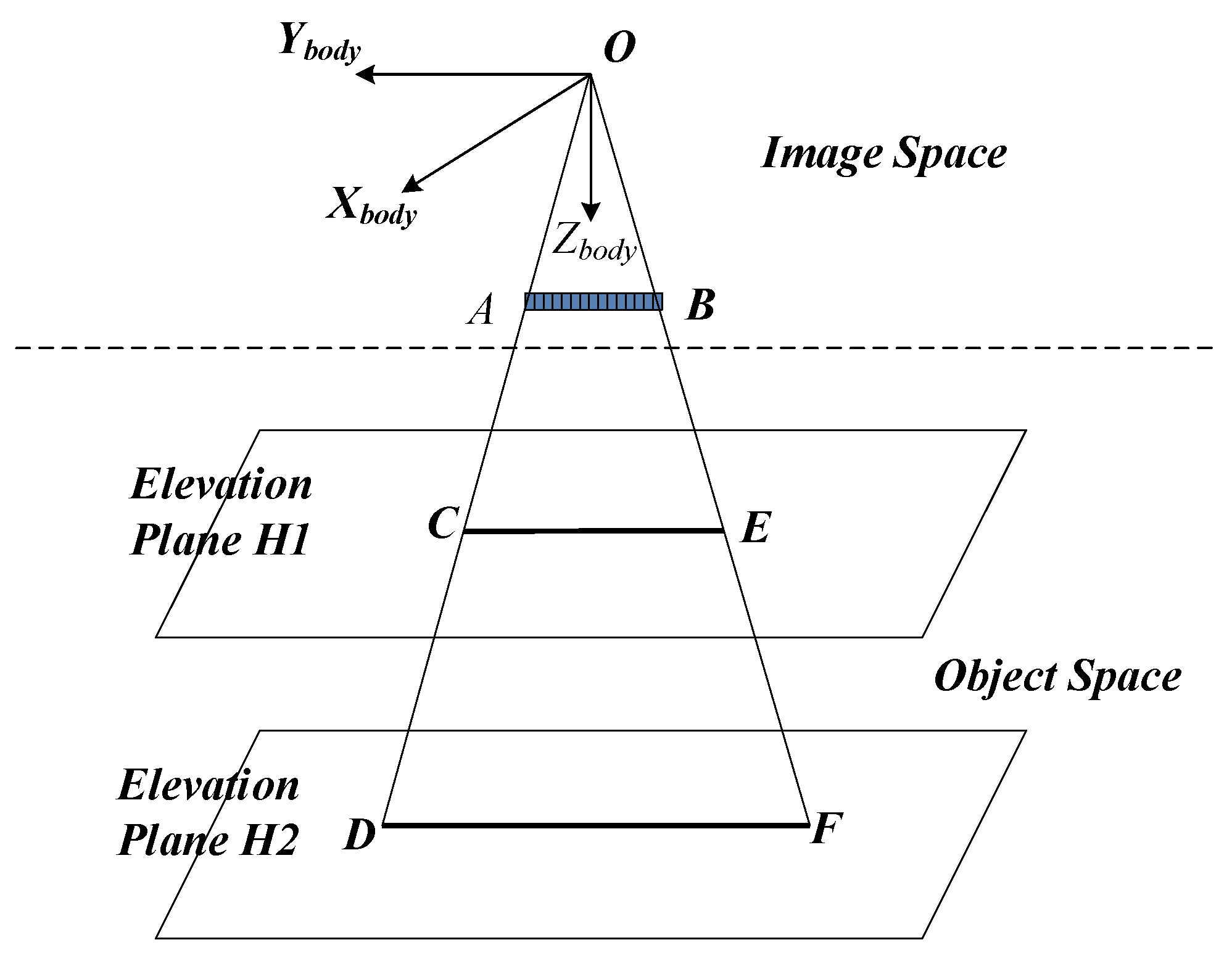
Recovering the RSM from the RFM is to obtain interior and exterior elements. The basic principle of recovering RSM from RFM is shown in
Figure 1. In the figure,
AB denotes the linear charge-coupled device (CCD) sensor at a certain time;
O denotes the position of the projection center, which is an unknown parameter;
OA and
OB are the rays at linear sensor ends.
XYZ stands for the satellite body-fixed coordinate system.
H1 and
H2 are two elevation planes whose elevations in the geodetic coordinate system are
H1 and
H2, respectively. The elevation plane
H1 intersects ray
OA at point
C and
OB at point
D; elevation plane
H2 intersects ray
OA at point
E and
OB at point
F.
Taking the detector A of the sensor AB at a specified time as an example, the ray OA intersects the elevation planes H1 and H2 at C and E in the object space, respectively. The geographical coordinates of C and E are and respectively. As the detector A is a common feature for ground points C and E, the image coordinates are both . and can be calculated by Equation (3). Then, the coordinates of C and E are and in geocentric Cartesian coordinate system, which can be derived from Equation (4). After the coordinates of C and E are determined, the direction of the ray in the Earth’s geocentric Cartesian coordinate system is the difference between the positions of C and E. This is the basic principle for using the RFM to recover the RSM. First, the position can be solved by the intersection of the vectors EC and FD. Based on the calculation result of the position, the attitude then can be calculated. Considering the correlation between the attitude and the interior orientation elements, the equivalent satellite body-fixed coordinate system is introduced, and its axis points to the ground direction which is the unit vectors of the rays OA and OB. The direction of the axis towards the flight, i.e., perpendicular to the plane OAB. The axis is determined by the axis and axis according to the right-hand criteria. When the axes of the three equivalent ontology coordinate systems are determined in the Earth’s geocentric coordinate system, can then be constructed. Finally, the direction of any ray in the satellite body-fixed coordinate system can be obtained through further applying the rotation matrix .
2.2. Geometric Calibration Model
The calibration model for the linear sensor model was established based on previous work [
2,
33,
34], and it is expressed in Equation (5):
where
represent the satellite position,
is the rotation matrix,
represent the ray direction,
m is the unknown scaling factor,
represent the unknown ground position,
is the offset matrix that compensates for the exterior errors, and
denotes the interior orientation elements.
2.2.1. Exterior Calibration Model
can be expanded to Equation (6):
where
,
, and
are rotation angles about the
,
, and
axes in the satellite body-fixed fixed coordinate system, respectively. The measurement errors of attitude and orbit are considered as constant errors within one standard scene, but a degree of random deviation occurs between several scenes imaged at different times, i.e., there are different
values for different images.
2.2.2. Interior Calibration Model
Considering that the optical lens distortion is the main cause of error in the interior orientation elements, it is possible to compensate for the interior orientation element error by establishing a lens distortion model. The optical lens distortion error is the deviation of the image coordinates from the ideal coordinates caused by the lens design, fabrication, and assembly. It mainly includes the principal point error
, principal distance error
, radial distortion error
, and decentering distortion error
. Assuming that the principal point offset is
and the principal distance is
, the lens distortion model can be described as follows:
Let
, and then the distortion model can be described as follows:
where
. For the linear array sensor, where the image coordinate along the track is a constant value, and thus, is set as
, the above distortion model can be simplified as follows:
Equation (9) is the distortion model for the compensation of the interior orientation elements. The solving of the compensation model parameters is performed by solving the unknown numbers
,
,
,
,
,
,
, and
to achieve the compensation for the interior orientation elements. While Equation (9) is a relatively complex non-linear model, there must be an initial value assignment and iterative convergence problems and the stability of the solution will be relatively poor. In order to simplify the solution, Equation (9) can be expanded as follows:
and the following variable substitutions are performed:
Then Equation (10) can be simplified as follows:
Therefore, the above distortion model can be expressed as a quintic polynomial model of the image column variables. The polynomial model is as follows:
where variables
and
are parameters describing the distortion to be calculated,
s is the image coordinate across the track, and
l is the image coordinate along the track. It should be noted that the polynomial distortion model can be considered as a one-variable function related to the sample for the linear push-broom camera. Besides,
and
are not related because the along-track and across-track aberrations in the across-track direction are described independently.
2.3. Solution for Calibration Parameters
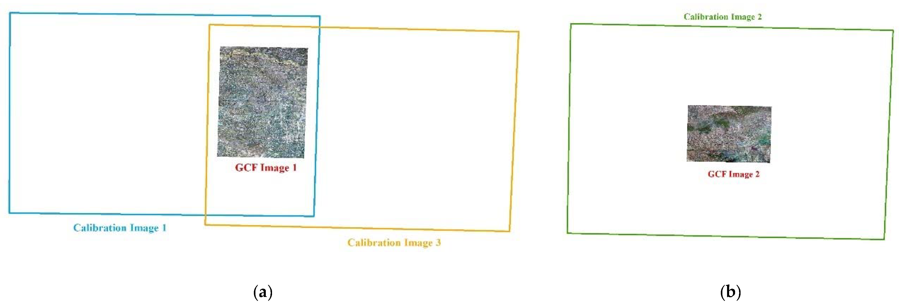
Calibration parameters can be calculated by high-precision GCPs obtained from the geometric calibration field (GCF) image by a high-accuracy matching method. However, on some occasions such as when processing images from a wide-field view camera, it is difficult to obtain sufficient GCPs for the reason that current GCFs fail to cover all rows in only one calibration-wide swath image. Therefore, multiple calibration images are collected to obtain sufficient GCPs covering all the rows. Multiple GCFs cover different parts of these calibration images, which extends the coverage of the GCF information accordingly. As shown in
Figure 2, with GCF image 1 covering the right half of calibration image 1 and the left half of calibration image 3, and with GCF image 2 covering the middle part of calibration image 2, all rows in the calibration image can be further covered by the GCF image.
Because multiple calibration images are acquired at different times, there are different exterior orientation elements but the same interior orientation elements for these images. Therefore, it is essential to apply exterior calibration for multiple calibration images before solving the interior orientation element errors. However, owing to the strong correlation between exterior and interior calibration parameters, the compensation residuals of exterior calibration parameters of different images inevitably affect the rightness of interior calibration parameters, i.e., there exists residuals after the compensation of the exterior orientation element errors.
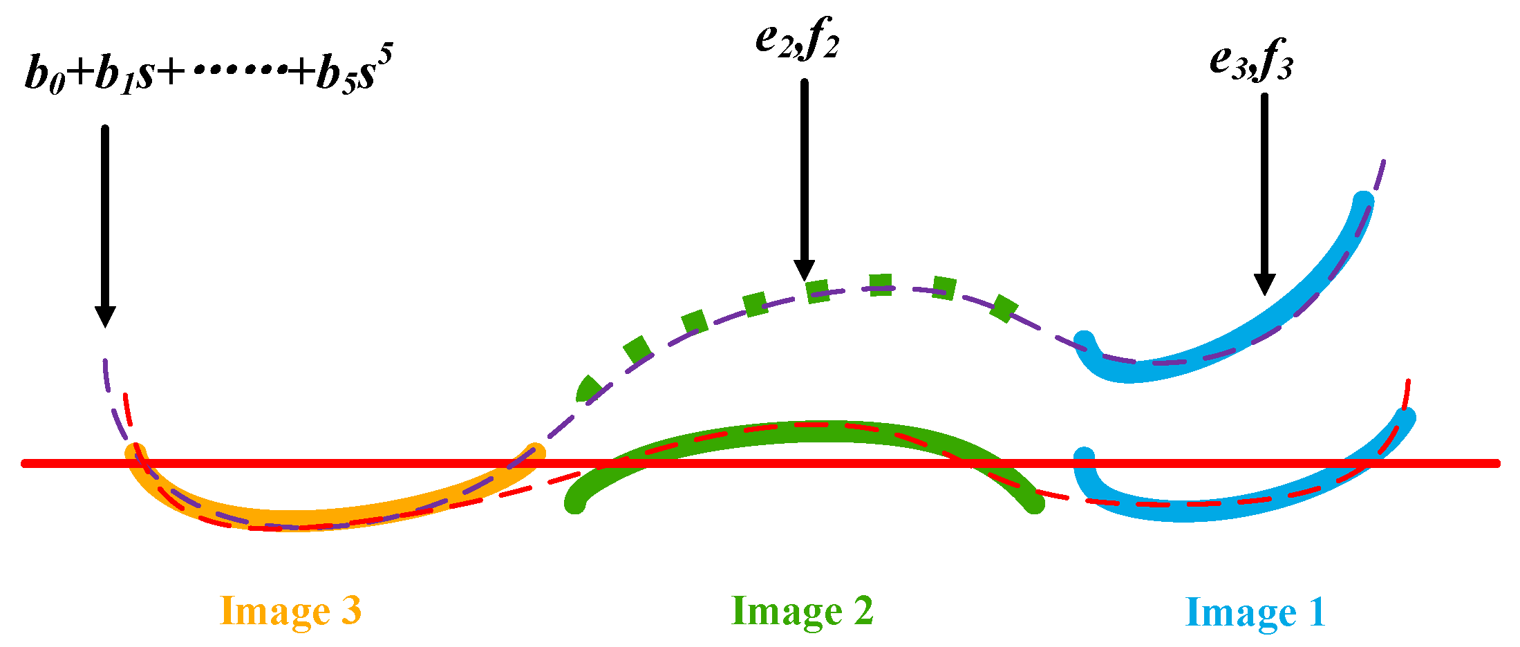
As shown in
Figure 3, after three calibration images being compensated by the exterior calibration parameters, taking the across-track error of the calibration image as an example, the residual curve is shown by the solid curve in the diagram (orange, green, blue). The red solid line in the figure is the baseline with an error of zero. It can be seen from the figure that the residual curves of the three calibration images are not continuous (as shown by the red dotted line in the figure) after the compensation of the exterior element errors. Therefore, the interior orientation element errors in the calibration image plane are difficult to fit by Equation (13).
According to [
23], when the attitude angle is small, the offset in the image plane caused by the exterior orientation element errors can be described by the shift, shift and scale, affine, and polynomial models. Since the calibration images have been compensated by the exterior calibration parameters, the exterior orientation element errors are much smaller than the previous ones and the residual exterior error can be described by the above model. When considering the orbit error, roll angle error, pitch angle error, and yaw angle error, the orientation error can be described as follows:
where
and
represent the orientation error caused by the residual exterior error,
S represents the orbit error,
represents the offset caused by the pitch angle error,
represents the yaw angle error,
s represents the sample index of a pixel, and the footnotes
l and
s represent the along-track and across-track values, respectively.
Therefore, in accordance with Equation (14), additional parameters (
e,
f) are introduced into the polynomial model across the track, which are used to describe the residuals of shift and rotation in the interior orientation elements compensation model. Normally, a calibration image is not introduced, such as calibration image 3 in
Figure 3, for computational stability. When these additional parameters are introduced and involved in the adjustment calculations, the other calibration image can be shifted and rotated, and then consequently the resulting residual curve can become continuous (as shown by the red dotted line in
Figure 3). The above computational solution process can be seen as an indirect adjustment with a constraint condition, where
b0,
b1,
b2,
b3,
b4,
b5 are the parameters to be requested, and
ej and
fj are the additional parameters that make the results more reasonable. This is also applicable for the residuals along the track.
Based on the above analysis, the system error compensation model with constrained conditions can be described as follows:
where
n denotes the number of calibration images participating in the adjustment calculation, and
cj,
dj,
ej,
fj denote additional parameters for each calibration image other than the reference calibration image.
5. Conclusions
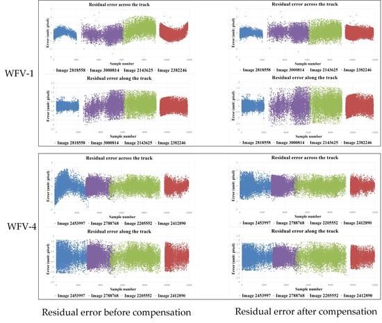
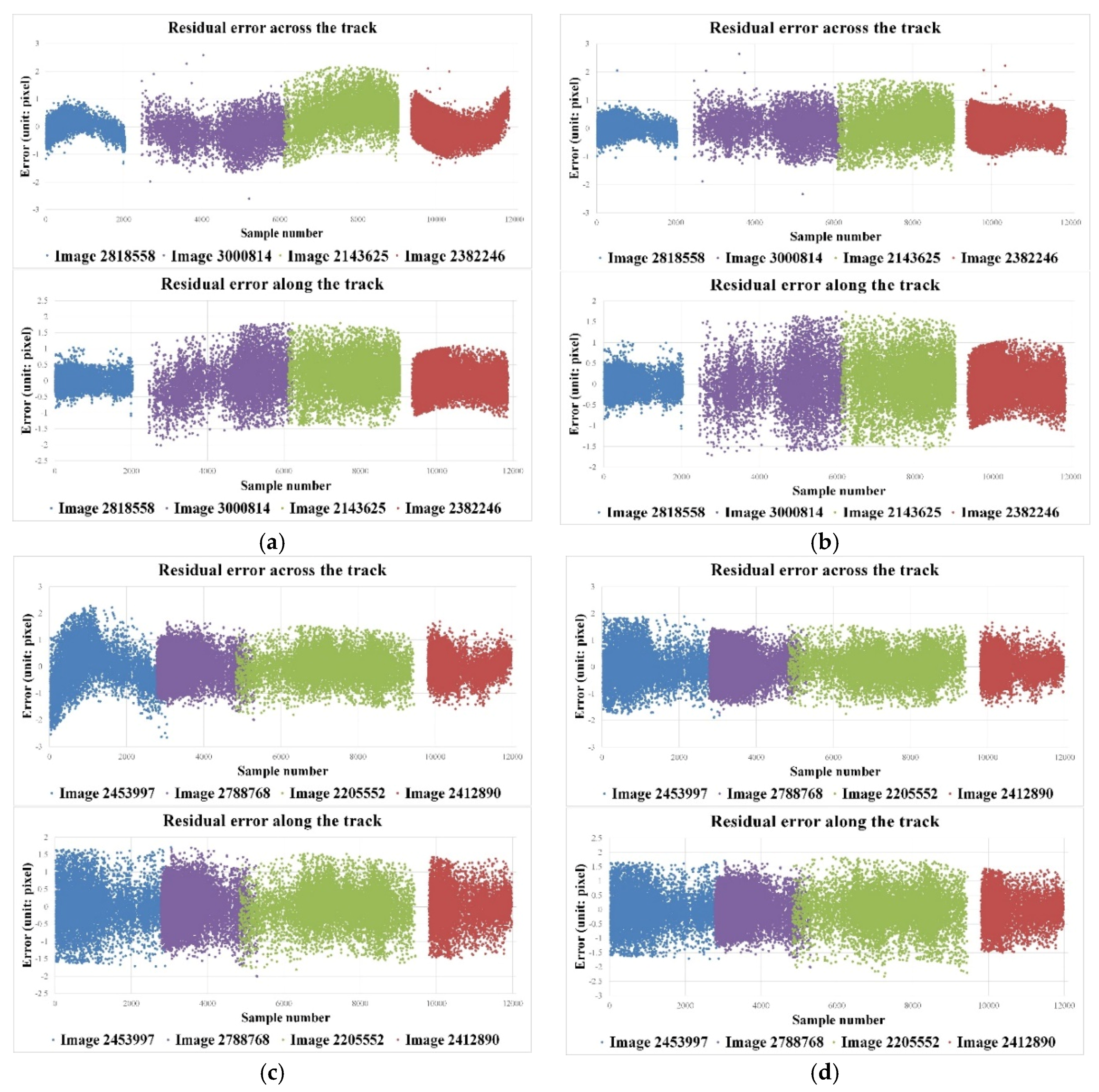
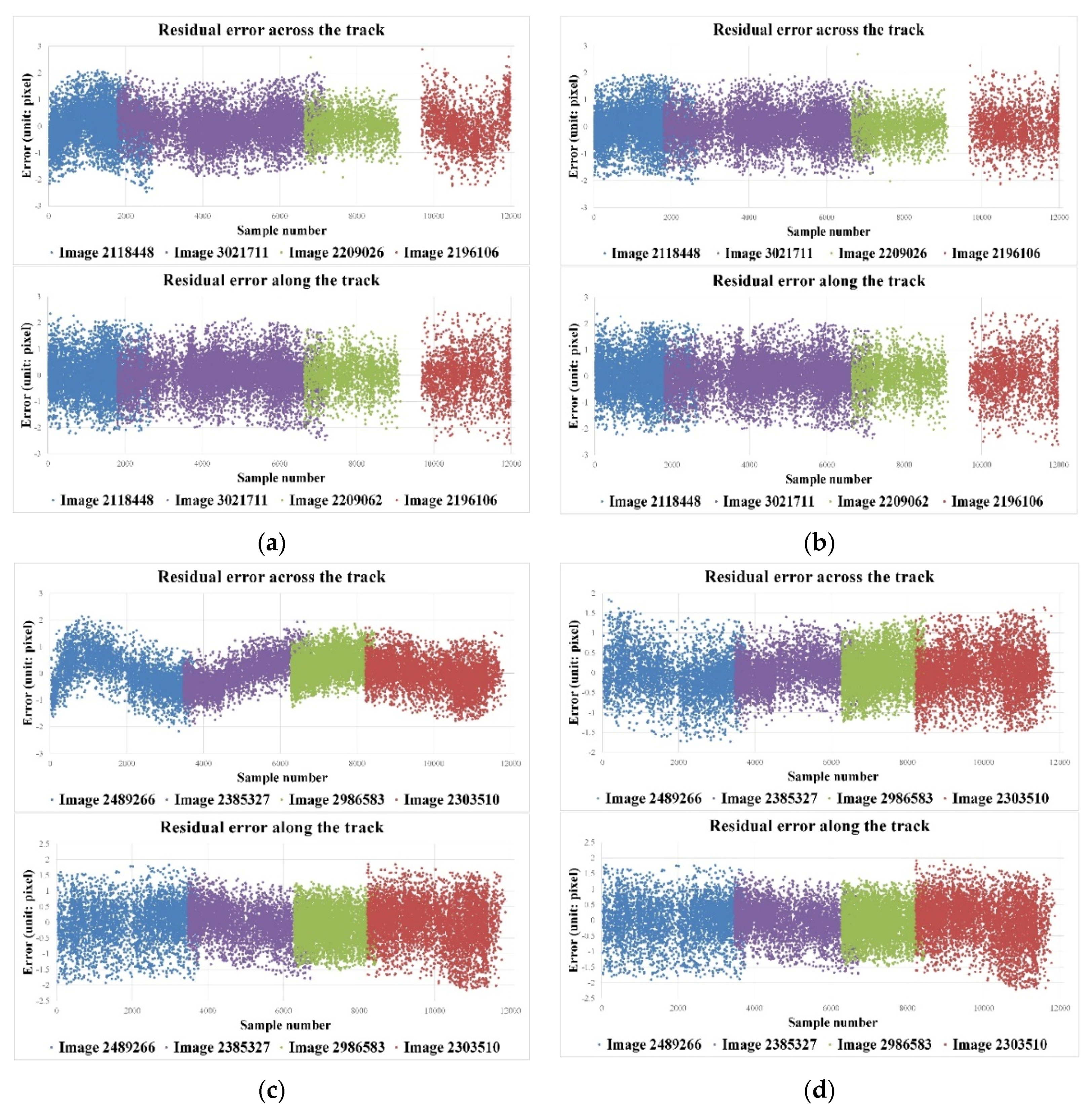
In this paper, a novel method was proposed to improve the geometric performance for a non-cartographic satellite’s imagery. Unlike conventional BCM methods, this method compensates for the system errors based on their cause rather than by simply building a compensation model according to the fit or to approximate the residuals. The proposed method recovers the RSM from the RFM first, and then it compensates for the system errors of the non-cartographic satellite’s images by using the conventional geometric calibration method based on the RSM; finally, a new and improved RFM is generated. Images captured by the WFV-1 camera and WFV-4 camera onboard GF-1 were collected as experimental data. Several conclusions can be drawn from the analysis, and these can be summarized.
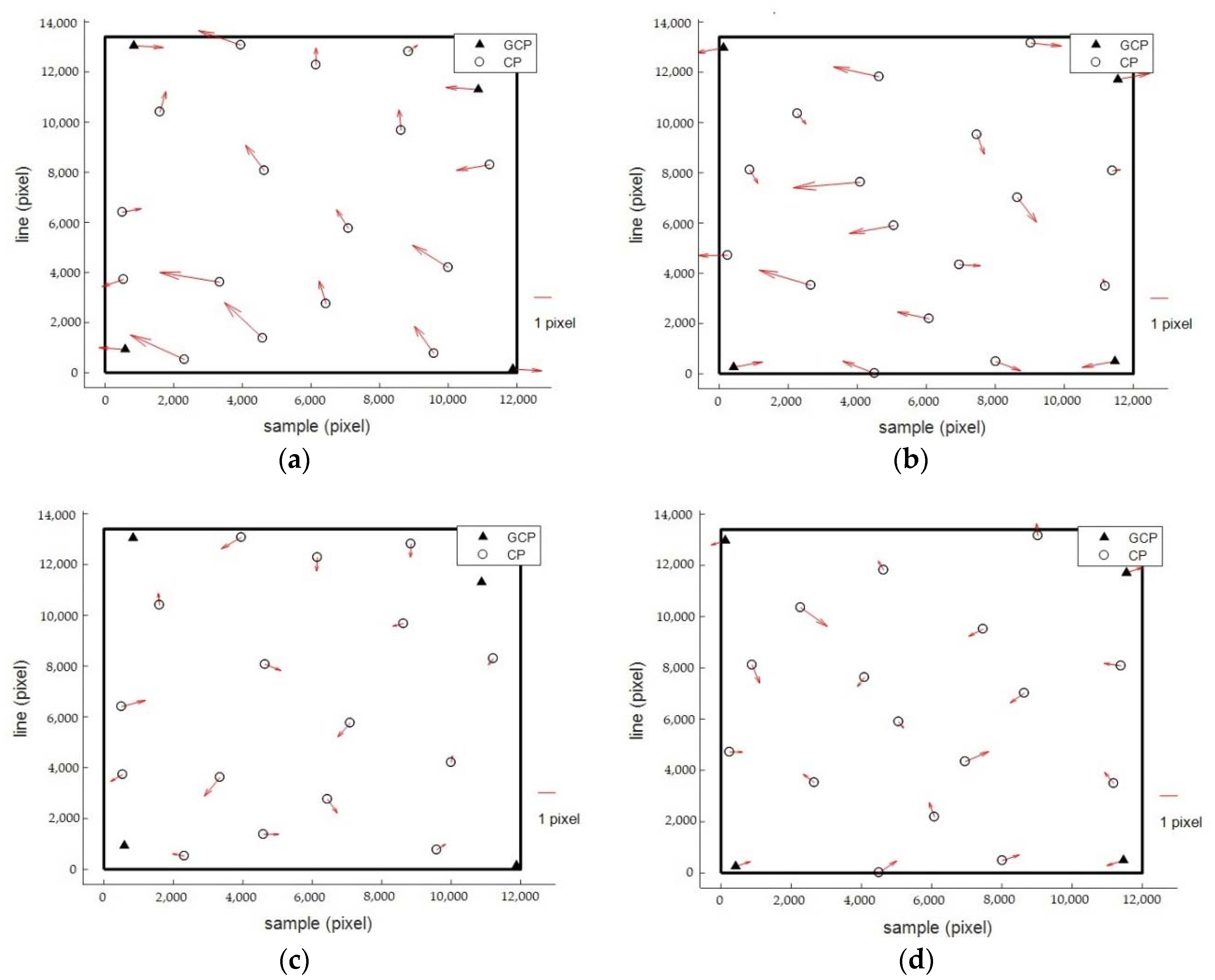
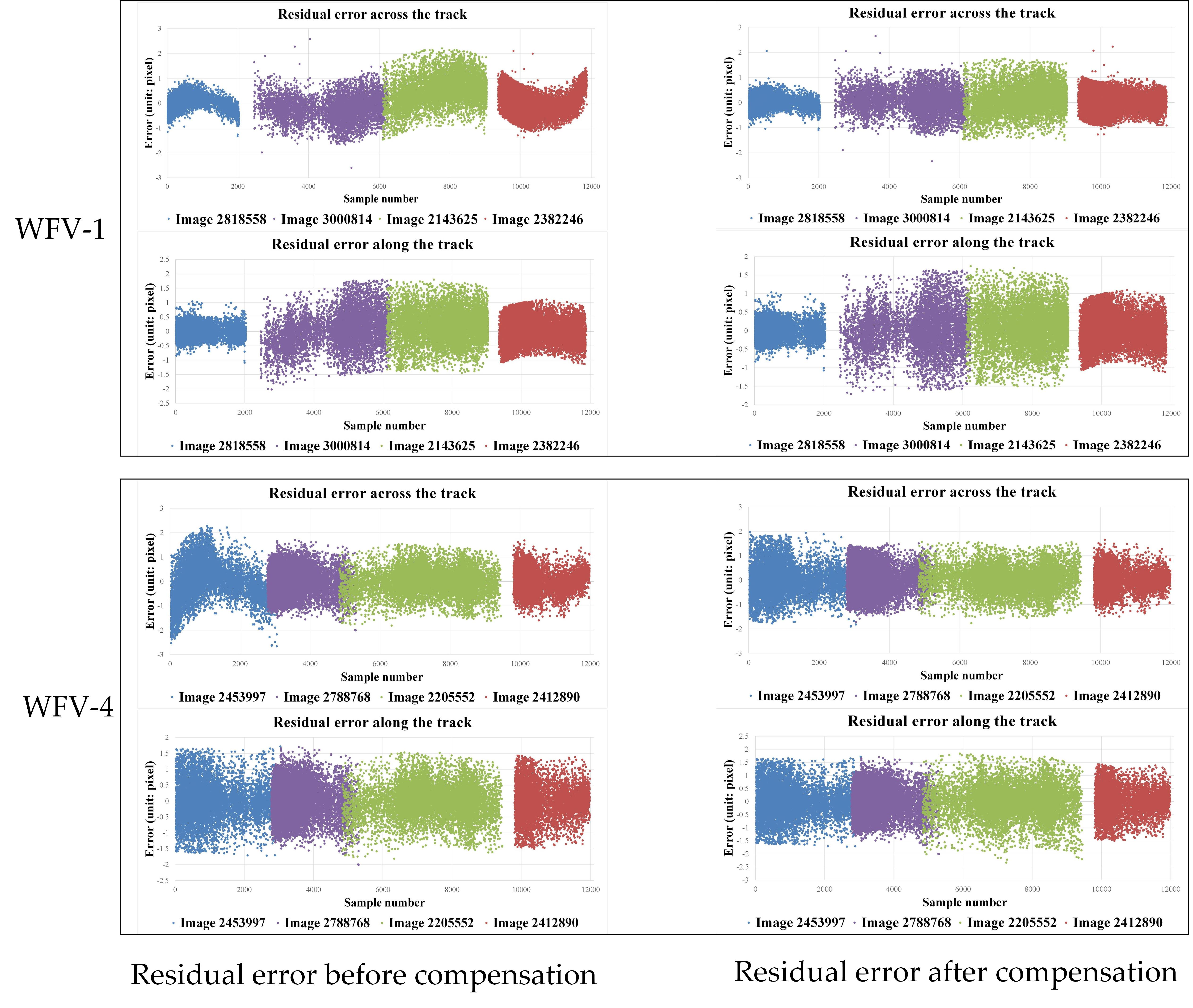
There exist obvious non-linear system errors across the track for GF-1 WFV images before applying the compensation, which adversely affect the potential for using the data in surveying and mapping applications and thus reduce the application effectiveness of Earth observation data. After employing this proposed method, images exhibited superior orientation accuracy compared to the original ones. Experiments demonstrated that the orientation accuracy of the proposed method evaluated by CPs was within 1 pixel for both the calibration images and validation images, and the residual errors manifested in a random distribution. Validation by using the CPs obtained via photographs taken in aerial photography field work further proved the effectiveness of the proposed method, and the entire scene was undistorted compared to that without applying the calibration parameters. Moreover, for the validation of the elevation accuracy, block adjustment tests showed that the vertical accuracy had improved from 21 m to 11 m with four GCPs, and these values were coincident with the theoretical values. Generally, these findings demonstrate the potential of using a non-cartographic optical remote-sensing satellite’s images for mapping by the proposed method.


